


| Issue |
A&A
Volume 711, July 2026
|
|
|---|---|---|
| Article Number | A118 | |
| Number of page(s) | 21 | |
| Section | Interstellar and circumstellar matter | |
| DOI | https://doi.org/10.1051/0004-6361/202659140 | |
| Published online | 08 July 2026 | |
ALMAGAL
IX. The chemical complexity of AG318.9477−00.1960: A line-identification template for ALMAGAL
1
Università degli Studi di Firenze,
Via G. Sansone 1,
50019
Sesto Fiorentino,
Firenze,
Italy
2
INAF-Osservatorio Astrofisico di Arcetri,
Largo E. Fermi 5,
50125
Firenze,
Italy
3
Centro de Astrobiología (CAB), CSIC-INTA,
Ctra. de Ajalvir, km. 4, Torrejón de Ardoz,
28850
Madrid,
Spain
4
Institut de Ciències de l’Espai (ICE), CSIC,
Campus UAB, Carrer de Can Magrans s/n,
08193,
Bellaterra, Barcelona,
Spain
5
Institut d’Estudis Espacials de Catalunya (IEEC),
08860
Castelldefels, Barcelona,
Spain
6
University of Connecticut, Department of Physics,
196A Auditorium Road Unit 3046,
Storrs,
CT
06269,
USA
7
INAF-Istituto di Astrofisica e Planetologia Spaziale,
Via Fosso del Cavaliere 100,
00133
Roma,
Italy
8
Max Planck Institute for Astronomy,
Königstuhl 17,
69117
Heidelberg,
Germany
9
National Radio Astronomy Observatory,
520 Edgemont Rd,
Charlottesville
VA
22903,
USA
10
Departamento de Astronomía, Universidad de Chile,
Casilla 36-D,
Santiago,
Chile
11
Department of Physics, National Cheng Kung University,
No. 1, University Road,
Tainan City
70101,
Taiwan
12
Jodrell Bank Centre for Astrophysics,
Oxford Road, The University of Manchester,
Manchester
M13 9PL,
UK
13
I. Physikalisches Institut, Universität zu Köln,
Zülpicher Straße 77,
50937
Köln,
Germany
14
Institute of Astronomy and Astrophysics, Academia Sinica,
11F of ASMAB, AS/NTU No. 1, Sec. 4, Roosevelt Road,
Taipei
10617,
Taiwan
15
East Asian Observatory,
660 N. A’ohoku, Hilo,
Hawaii,
HI
96720,
USA
16
School of Engineering and Physical Sciences, Isaac Newton Building, University of Lincoln,
Brayford Pool,
Lincoln
LN6 7TS,
UK
17
Korea Astronomy and Space Science Institute,
776 Daedeokdae-ro, Yuseong-gu,
Daejeon
34055,
Republic of Korea
18
University of Science and Technology, Korea (UST),
217 Gajeong-ro, Yuseong-gu,
Daejeon
34113,
Republic of Korea
19
UK Astronomy Technology Centre, Royal Observatory Edinburgh,
Blackford Hill,
Edinburgh
EH9 3HJ,
UK
20
Universität Heidelberg, Zentrum für Astronomie, Institut für Theoretische Astrophysik,
Albert-Ueberle-Str. 2,
69120
Heidelberg,
Germany
21
Universität Heidelberg, Interdisziplinäres Zentrum für Wissenschaftliches Rechnen,
Im Neuenheimer Feld 225,
69120
Heidelberg,
Germany
22
Faculty of Physics, University of Duisburg-Essen,
Lotharstraße 1,
47057
Duisburg,
Germany
23
Jet Propulsion Laboratory, California Institute of Technology,
4800 Oak Grove Drive,
Pasadena,
CA
91109,
USA
24
Dipartimento di Fisica, Università di Roma Tor Vergata,
Via della Ricerca Scientifica 1,
00133
Roma,
Italy
25
SRON Netherlands Institute for Space Research,
Landleven 12,
9747 AD
Groningen,
The Netherlands
26
Kapteyn Astronomical Institute, University of Groningen,
9700 AV
Groningen,
The Netherlands
27
Center for Data and Simulation Science, University of Cologne,
Germany
28
Center for Astrophysics | Harvard & Smithsonian,
60 Garden Street,
Cambridge,
MA,
02138,
USA
29
Research Center for Computational Earth and Space Science, Zhe-jiang Laboratory,
Hangzhou,
China
★ Corresponding author: This email address is being protected from spambots. You need JavaScript enabled to view it.
Received:
26
January
2026
Accepted:
11
May
2026
Abstract
Context. High-mass star-forming regions are rich in complex organic molecules (COMs), which are carbon-bearing species with at least six atoms. Their formation pathways remain debated. The ALMA evolutionary study of high-mass protocluster formation in the GALaxy (ALMAGAL) survey provides a unique opportunity to probe this chemical complexity in a large statistical significant sample of high-mass star-forming regions.
Aims. We present a detailed molecular line analysis of one of the most chemically rich cores in the ALMAGAL sample, the high-mass core 9 in the AG318.9477−00.1960 clump (AG318−c9), located at a heliocentric distance of ∼10.4 kpc. This source was selected because it combines an exceptionally high line density with a relatively simple kinematic structure, making it an optimal template for chemical analysis in the survey. We further assessed whether the emission of selected COMs, that is, ethylene glycol ((CH2OH)2; EG), glycolaldehyde (CH2(OH)CHO; GA), and methyl formate (CH3OCHO; MF), can be used to trace the innermost regions of hot molecular cores (HMCs).
Methods. We analysed ALMA Band 6 observations (∼217–221 GHz). Spectral line identification and local thermodynamic equilibrium modelling were performed using the software called MAdrid Data CUBe Analysis (MADCUBA). We derived the physical parameters, including the column density (N), excitation temperature (Tex), velocity, line width, and molecular abundances relative to H2, for all detected species. The chemical inventory of AG318−c9 was compared with that of the HMC G31.41 + 0.31 (G31). In addition, we performed a pixel-by-pixel analysis of EG, GA, and MF to generate spatially resolved N and Tex maps and corresponding radial profiles.
Results. We report the detection of 65 molecular species, including 31 main species and 34 isotopologues and vibrationally excited species. Of these, 44 are O-bearing species, 28 are N-bearing, 8 are S-bearing, and 2 are Si-bearing. While AG318−c9 exhibits lower abundances than G31 overall, it shows detections of species that have not yet been reported in G31, such as ethyl formate (C2H5OCHO). Moreover, 12 species depart from the general trend, displaying relative overabundances in AG318−c9. The comparison also reveals a chemical differentiation between O- and N- bearing COMs, with O-bearing species systematically more abundant in G31. Regarding EG, GA, and MF, the latter is the most abundant (X ∼ 3 × 10⁻⁸), followed by EG (X ∼ 7 × 10⁻⁹) and GA (X ∼ 2 × 10⁻⁹). The N and Tex maps suggest that MF is the most spatially extended species, whereas EG and GA are more compact and confined to the innermost hot region.
Conclusions. AG318−c9 reveals a rich chemical inventory characteristic of an HMC. The chemical comparison with G31 suggests that AG318−c9 is a less evolved hot core dominated by the recent sublimation of ice mantles, in contrast to the higher abundances observed in the possible more evolved G31. MF emerges as an excellent tracer of the gas temperature in HMCs owing to its wide spatial extent and wide dynamic range of the excitation temperature. In contrast, EG and GA are more compact and preferentially trace the innermost high-density regions of the core, suggesting a high sublimation temperature threshold and supporting a shared grain-surface formation pathway. While EG and MF seem to be partly limited by sensitivity, GA reflects an intrinsically central distribution.
Key words: astrochemistry / line: identification / stars: formation / stars: massive / ISM: molecules / ISM: individual objects: AG318.9477−00.1960
© The Authors 2026
 Open Access article, published by EDP Sciences, under the terms of the Creative Commons Attribution License (https://creativecommons.org/licenses/by/4.0), which permits unrestricted use, distribution, and reproduction in any medium, provided the original work is properly cited.
This article is published in open access under the Subscribe to Open model. This email address is being protected from spambots. You need JavaScript enabled to view it. to support open access publication.
1 Introduction
Astrochemistry is inherently a multidisciplinary field that involves physics, chemistry, biology, and geology to investigate the formation and evolution of molecules in the interstellar medium (ISM). Unveiling the chemistry in a particular environment provides crucial insight into the emergence of molecular complexity, the dominant chemical processes, and how these are inherited at different evolutionary stages. Furthermore, astro-chemical studies provide constraints on the physical conditions and lifetimes of these regions (Jørgensen et al. 2020). At its core, astrochemistry studies the potential precursors of life, and together with astrobiology, addresses one of the most fundamental open questions in science: the origin of life.
As of November 2025, approximately 340 molecules have been detected in the ISM or in circumstellar shells (Müller 2025). They include the so-called complex organic molecules (COMs), which are defined as carbon-bearing species with at least six atoms (Herbst & van Dishoeck 2009). COMs play a central role as they represent key steps towards increasing chemical complexity, potentially leading to the formation of prebiotic species. The latter are regarded as building blocks of life, as they share structural elements with biomolecules found in living organisms and are thought to play a role in prebiotic chemical processes (Caselli & Ceccarelli 2012; Ceccarelli et al. 2022).
Although the formation of COMs remains under debate, two main and potentially complementary pathways have been proposed: (i) surface reactions on interstellar dust grains (Simons et al. 2020; Garrod et al. 2022), and (ii) gas-phase chemical reactions (Balucani et al. 2015; Skouteris et al. 2018). During the early stages of star formation, cold molecular clouds are characterised by temperatures of ∼10–20 K and densities of ∼103–104 cm−3, which increase as the cloud evolves and collapses. With these conditions, atoms and simple species such as oxygen, nitrogen, and hydrogen accrete onto dust grains, forming icy mantles. In this scenario, grain-surface chemistry is dominated by hydrogenation reactions, leading to a chemical inventory dominated by simple species such as water (H2O), methane (CH4), or ammonia (NH3; Tielens 2013; Boogert et al. 2015; Linnartz et al. 2015). As collapse proceeds and densities reach ∼104–106 cm−3, significant CO freeze-out occurs, enabling CO hydrogenation and the formation of species such as the formyl radical (HCO), formaldehyde (H2CO), and eventually, methanol (CH3OH), the simplest and most abundant COM (Watanabe & Kouchi 2002; Fuchs et al. 2009; Santos et al. 2022). Moreover, ultraviolet photons and cosmic rays enable the gradual build-up of molecular complexity (Öberg 2016; Padovani et al. 2020). As material accretes onto the protostar, the resulting accretion shocks significantly increase the central luminosity and raise the envelope temperature from 10 K to 100–300 K. This thermal processing triggers the sublimation of icy mantles from dust grains, releasing species into the gas phase (Caselli & Ceccarelli 2012). When they are in the gas phase, COMs can be detected with radio telescopes via their characteristic rotational transitions.
The COMs are commonly observed in high-mass star-forming regions at different evolutionary stages due to high gas densities, intense heating occurring during the hot molecular core (HMC) phase, and efficient desorption processes that enhance their detectability and abundance (Baek et al. 2022; Coletta et al. 2020). HMC regions have the richest chemistry in the Galaxy (Bisschop et al. 2007; Belloche et al. 2013; Rivilla et al. 2017). In addition to tracing chemical complexity, COMs probe a wide range of physical conditions (temperature and density) and provide valuable insights into the physical properties, kinematics, and formation mechanisms of high-mass star-forming regions. In this context, heavy COMs (those with ≥ 8 atoms) and prebiotic species are typically less abundant and more optically thin than standard HMC tracers such as CH3CN, allowing them to better probe the innermost densest regions of high-mass cores (Rivilla et al. 2017).
However, it remains challenging to detect COMs because their emission is generally weaker than that of simpler and more abundant species. In chemically rich regions, spectra can become so densely populated with molecular transitions that individual lines overlap and cannot be uniquely identified, reaching the line-confusion limit, where increased sensitivity no longer enables secure detections of weaker species. This effect is particularly severe in turbulent environments. Consequently, a careful and detailed line identification is required to reliably assign molecular transitions and derive the physical properties of less abundant species.
Motivated by these considerations, we performed an exhaustive line identification towards core 9 of the AG318.9477−0.1960 clump (hereafter AG318−c9; Fig. 1), which is one of the most chemically rich cores in the ALMA evolutionary study of high-mass protocluster formation in the Galaxy (ALMA-GAL) large project (2019.1.00195.L; Molinari et al. 2025; Sánchez-Monge et al. 2025). ALMAGAL is a survey of high-mass star-forming regions in the Galactic plane that are observed with the Atacama Large Millimetre Array (hereafter ALMA; Wootten & Thompson 2009) in Band 6 (Kerr et al. 2004). The survey was selected from the Herschel Infrared Galactic Plane Survey (Hi-GAL, Molinari et al. 2016; Elia et al. 2018, 2021) and Red MSX Source survey (RMS; Hoare et al. 2005; Urquhart et al. 2007; Lumsden et al. 2013) catalogues. By observing 1013 dense clumps in various evolutionary stages and Galactic environments, ALMAGAL provides a statistically significant and uniformly observed sample to investigate the physical and chemical evolution of high-mass star-forming regions. Detailed descriptions of the ALMAGAL survey characterisation (Molinari et al. 2025), dataset and data reduction pipeline (Sánchez-Monge et al. 2025), fragmentation properties of the compact sources (Coletta et al. 2025), and early scientific results (Wells et al. 2024; Mininni et al. 2025; Elia et al. 2026; Schisano et al. 2026; Wallace et al. 2026) are available.
In a forthcoming study (Allande et al., in prep.), we will analyse the emission of three potentially chemically related COMs across the full ALMAGAL sample: GA, EG, and MF. Laboratory experiments and astrochemical models indicate that GA and EG are chemically linked and may share common formation pathways in the ISM (Sorrell 2001; Fedoseev et al. 2015; Coutens et al. 2018; Garrod et al. 2022). MF, while not directly connected through the same synthetic routes, is the most abundant isomer of GA and provides complementary constraints on the formation of GA and EG, as all three species are expected to arise under similar physical conditions (Simons et al. 2020).
As a necessary first step towards this survey-wide analysis, we present a detailed line identification of the ALMAGAL spectral band coverage (216.98–218.86 GHz and 219.06–220.94 GHz) towards AG318−c9. We identify all detectable molecular species contributing to the emission in this frequency range and perform an initial analysis of the physical properties of GA, EG, and MF, with particular emphasis on assessing line blending and selecting the least affected transitions for further study. In addition, we explore the feasibility of deriving spatially resolved physical parameter maps (column density and excitation temperature) for these species, evaluating their potential as tracers of the physical conditions of dense gas (Rivilla et al. 2017; Nazari 2026).
This study therefore serves multiple purposes within the framework of the ALMAGAL survey. First, it provides a detailed characterisation of the chemical inventory of one of the most chemically rich HMCs in the sample. Second, it provides a robust and reproducible template for molecular line identification and analysis that can be consistently applied to the full ALMAGAL dataset. Third, by carefully assessing line blending effects affecting GA, EG, and MF, this work ensures a reliable derivation of their physical parameters and supports forthcoming survey-wide analyses. Finally, the spatially resolved analysis of these species enables us to evaluate their ability to trace the innermost warm and dense regions of HMCs, where COM chemistry is expected to be most active.
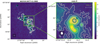 |
Fig. 1 ALMA map of the continuum emission at 1.38 mm of the AG318.9477−0.1960 clump (left) and a zoom-in on core 9 (right). The white contours correspond to 5σ, 10σ, 20σ, 30σ, 60σ, 90σ, 180σ, 220σ, and 260σ, with σ ∼ 0.28 mJy beam−1. The cyan ellipses surrounded by black show the position and size of each core. In particular, the size of core 9 is 0.″66 × 0.″57, with a position angle of PA=42°. The synthesised beam (0.″46 × 0.″37, PA=7°) is shown in the bottom left corner. |
Properties of the core AG318−c9.
2 The source
2.1 AG318.9477−00.1960 clump
AG318.9477−0.1960 is a high-mass clump located at a heliocentric distance of DHEL ∼ 10.4 ± 0.4 kpc and a Galactocentric distance of DGAL ∼ 6.84 kpc. It is centred at αclump(ICRS) = 15h 00m 55.s293 and δclump(ICRS) = −58° 58′ 52.″511. The clump has a mass of Mclump ∼ 5870 M⊙, a luminosity of Lclump ∼ 2.7 × 10⁵ L⊙, an L/M ∼46.5 L⊙/M⊙, and a systemic velocity of Vlsr = −34.4 km s−1 (Molinari et al. 2025).
The source is associated with compact mid-IR and far-IR emission, indicating a dense and embedded environment. The radio continuum emission observed with the Australia Telescope Compact Array (ATCA) at 5.5–22.8 GHz detected unresolved free-free emission with a rising spectral index of α = 0.69±0.22, which was interpreted as arising from a partially optically thick conical non-collimated radio jet (Purser et al. 2016). The possibility that the free-free emission is associated with an HII region was dismissed based on the low radio luminosity measured at 22.8 GHz, which is only 1.4% of that expected for an optically thin HII region. Additional evidence of jet activity includes aligned knots of H2 emission (Lee et al. 2001; De Buizer 2003), a bipolar SiO outflow (De Buizer et al. 2009), and CH3OH masers at 36 GHz and 44 GHz (Voronkov et al. 2014).
2.2 Core 9
The compact cores embedded in the ALMAGAL clumps were identified with the structure identification algorithm CUrvature Thresholding EXtractor (CuTEx; Molinari et al. 2011) based on their integrated dust continuum flux. This algorithm has allowed us to identify 6348 cores in 844 of the 1013 ALMAGAL clumps (Coletta et al. 2025). By fitting Gaussians to each extracted core, Coletta et al. (2025) have estimated the dust continuum emission from the line-free channels and the size of the continuum emission. Within clump AG318.9477−0.1960, 19 compact cores were identified (Fig. 1), among which core 9 stands out as a particularly chemically rich source. We discuss the criteria used to choose this source among all the others in the ALMAGAL sample in 4.1 in detail. The properties of AG318−c9 are described in Table 1.
3 Observations
The ALMAGAL large project observed a total of 1013 targets using ALMA. The observations were carried out with the main 12 m array in two different configurations: an extended configuration (C-5 and C-6), and a compact configuration (C-2 and C-3), hereafter referred to as TM1 and TM2, respectively; (Escoffier et al. 2007). The observations were also carried out with the 7 m Atacama Compact Array (Iguchi et al. (2009); hereafter 7M). We used data that combine all three configurations (7M + TM1 + TM2), yielding a synthesised beam of 0.″46 × 0.″37 with a PA=7 °. For AG318−c9, this corresponds to physical scales of ∼4800 au × 3900 au along the major and minor axes, respectively.
The observations were conducted in ALMA Band 6 at ∼ 1.38 mm (∼217 GHz). The spectral setup comprised four spectral windows (spw). We used spw0 and spw1, each covering a bandwidth of 1.87 GHz with 3840 channels of 488 kHz, corresponding to a spectral resolution of ≈1.4 km s−1. These spectral windows cover the frequency ranges 216.98–218.86 GHz and 219.06–220.94 GHz, respectively. The remaining two spectral windows (spw2 and spw3), which cover narrower bandwidths of 0.468 GHz, were not considered here as they correspond to higher spectral resolution subwindows within the frequency ranges already covered by spw0 and spw1 and do not provide additional constraints for line identification, especially for weak species. The RMS noise of the continuum map is σ ≈ 0.28 mJy beam−1 (Coletta et al. 2025). A detailed description of the ALMAGAL data-processing workflow, including calibration, data staging, continuum determination, self-calibration, imaging, and data products, is provided in Sánchez-Monge et al. (2025).
4 Method
To study the richness of the spectral line emission of each core, we extracted the spectra in the two broad spectral windows (spw0 and spw1) by integrating the emission over the ellipse that describes the size of each continuum core. The core identification procedure is described in detail in the ALMAGAL core catalogue (Coletta et al. 2025).
4.1 Identification of the richest chemical core
We sorted the spectra of all the ALMAGAL cores using the intensity of the K = 2 component of methyl cyanide (CH3CN), where K denotes the projection of the total rotational angular momentum onto the principal axis of the molecule, at 220.730 GHz. This transition is one of the brightest in the spectral setup, is minimally affected by line blending, and is a well-established tracer of HMCs (e.g. Cesaroni 2005; Cesaroni et al. 2011). After sorting the spectra of the ALMAGAL cores, we found that sources with weak emission in the low-K components of CH3CN exhibit little or no complex chemistry, whereas sources with strong low-K CH3CN emission display chemically rich spectra, consistent with previous studies (e.g. G31.41+0.31; Beltrán et al. 2005; Mininni et al. 2020). We therefore selected sources with a very good signal-to-noise ratio (S/N) emission in the CH3CN K = 2 transition because weaker and less abundant species would otherwise not be reliably detected.
Since the forthcoming study will focus on GA, EG, and MF, we further considered the intensity of one of the brightest MF transitions in the observed band, the 173,14 → 163,13 at 218.298 GHz. The two selection criteria consistently place AG318−c9 among the cores with the highest S/N in the ALMA-GAL sample, supporting its use as a template source for detailed chemical analysis.
Moreover, we selected AG318−c9 as a representative chemically rich core within the ALMAGAL sample based on additional criteria. First, it exhibits a high line density of approximately ∼80 lines GHz−1 (Sánchez-Monge et al., in prep.). This line density is comparable to that observed in the most chemically rich cores of Sgr B2, one of the chemically richest regions in the Galaxy (Belloche et al. 2025). Second, AG318−c9 does not show strong multiple velocity components, which greatly facilitates reliable line identification and detailed spectral analysis. Third, AG318−c9 is the third most massive core in the sample. The two more massive cores were excluded because the most massive core shows prominent self-absorption features, while the second core exhibits highly noisy spectra.
4.2 Line identification
For the line identification in AG318−c9, we searched for molecular species with an S/N ≥ 5 (corresponding to ∼1.35 K) to ensure reliable detections. We first fitted species expected to be bright and abundant in HMCs, such as H2CO, CH3CN, or CH3OH, which simultaneously account for multiple of the brightest transitions in the observed frequency range. For the remaining unidentified lines, we used Splatalogue1 to search for additional molecular species with transitions consistent with the observed frequencies, drawing spectroscopic data from the CDMS2 (Müller et al. 2001, 2005; Endres et al. 2016) and the JPL3 (Pickett et al. 1998) catalogues.
To confirm or discard the identification of the different candidate species, we used the spectral analysis software Madrid data cube analysis (MADCUBA4; Martín et al. 2019). This software allowed us to identify and fit different species using the tool called spectral line identification and modeling (SLIM), which generates a synthetic spectrum under the assumption of local thermodynamic equilibrium (LTE) while accounting for line opacity. Given the high gas density of AG318−c9,  (Coletta et al. 2025), the assumption of LTE is well justified. The H2 column density,
  (Table 1), was derived using
  , where Mcore is the mass of the core, and Dcore = 6396 au is the geometric mean size of AG318−c9, as reported by Coletta et al. (2025). Here, mH = 1.67 × 10⁻²⁴ g is the hydrogen atom mass, and µ = 2.8 is the mean molecular weight per particle. This
  was then used to compute molecular abundances relative to H2 (
 ).
).
The synthetic spectra were generated and controlled by input physical parameters: column density (N), excitation temperature (Tex), radial velocity of the source (V), full width at half maximum (FWHM), and source size (θs). Best-fit solutions were obtained using the AUTOFIT routine, which performs a non-linear least-squares minimisation based on the Levenberg-Marquardt algorithm (Levenberg 1944; Marquardt 1963).
All detectable molecular species towards AG318−c9 were initially identified and fitted manually using MADCUBA. As we aimed to establish a framework for the chemical analysis of the full ALMAGAL sample, AG318−c9 was used as a testbed to develop a script that automates the line identification and fitting procedures (Appendix A). This automation facilitates the evaluation of individual molecular species in the survey, improving the robustness of the derived physical parameters and their associated uncertainties, particularly for fainter species, such as EG and GA. Although we attempted to derive all the physical parameters for each species, in some cases, AUTOFIT did not converge, and certain parameters had to be fixed. In particular, Tex was fixed to the value derived for MF  when only one transition was available or when the detected transitions did not span a sufficiently wide range of energies to converge in a solution. The full procedure is described in Appendix A.
The species for which we left Tex free generally span a wide range of energies, with minimum values typically of a few tens of kelvin and maximum values reaching several hundred kelvin. The widest Eup range was found for NH2CN (579 K), and the smallest range was found for CH3COOH (57 K).
Since EG, GA, and MF have clearly been detected in AG318−c9, we also generated N and Tex maps (Sect. 6.4). Pixel-by-pixel fitting of selected transitions was performed (Appendix B), allowing us to better constrain the physical conditions and chemical structure of the core.
Molecular species detected in core 9 of the AG318.9477−0.1960 clump.
5 Spectral line analysis
We present the complete chemical inventory analysed in AG318−c9 derived from the ALMAGAL frequency setup. To place these results, we compare them with those of the well-studied HMC G31.41+0.31.
5.1 Molecular inventory
The analysis of the spectra reveals molecular emission from a total of 65 different species (Table 2). This underlines the chemically rich environment in AG318−c9. Of these species, 31 correspond to rotational transitions of main species, and the remaining 34 species arise from isotopologues and vibrationally excited species. Figures 2 and 3 show the observed spw0 and spw1 spectra together with the global LTE fit, which accounts for the contribution of all identified species. Zoomed-in versions of the spectra, presented in Appendix C, illustrate the quality of the fits for weaker transitions. Despite the large number of detected species, not all observed spectral features could be reliable identified. A total of 91 lines remained unassigned and are labelled unidentified (U) in the spectra. Although the most recent CDMS and JPL catalogues were used, some of these unidentified features may correspond to transitions that are not yet included in current laboratory spectroscopic databases.
Overall, the identified molecular inventory reveals a chemically rich environment dominated by oxygen-bearing species (44), followed by nitrogen-bearing (28), sulphur-bearing (8), and silicon-bearing (2), with COMs accounting for more than half of the detections (33). In particular, GA, EG, and MF were identified through multiple transitions with good S/N ratios (≥ 5), of which 3, 8, and 14 transitions, respectively, were unblended. Additional heavy COMs, such as acetone (CH3COCH3) and ethyl formate (C2H5OCHO), are also present.
Remarkably, this rich chemical inventory is revealed by covering a narrow spectral setup of 4 GHz and with short integration times. The number of different species detected in AG318−c9 is comparable with those detected towards typical chemically rich HMCs such as G31.41+0.31, Sgr B2, and IRAS 16293−2422. However, the inventory of species in these well-known HMCs has been built through large unbiased spectral surveys: e.g., the GUAPOS survey (G31.41+0.31 Unbiased ALMA sPectral Observational Survey; Mininni et al. 2020) and the EMoCA survey (Exploring molecular complexity in the Galactic Centre with ALMA; Belloche 2017), which both span nearly the entire ALMA Band 3 (∼32 GHz), and the PILS survey (The ALMA Protostellar Interferometric Line Survey; Jørgensen et al. 2016) from 329 to 363 GHz (∼34 GHz), allowing a more complete census of molecular species. All this suggests that AG318−c9 is a chemically reference HMC within the ALMAGAL survey that might be as rich as other well-known and studied sources.
The detected species span a wide range of molecular complexity, from simple diatomic molecules such as the isotope of carbon monoxide 13CO to molecules with 11 atoms such as ethyl formate (C2H5OCHO). The complete list of identified species and their correspondent transitions is available in a repository table5. Together, this inventory supports the classification of AG318−c9 as a chemically rich HMC.
For all identified species, we derived the column density, excitation temperature, velocity, line width, and abundance (Table 3), following the procedure described in Appendix A. The excitation temperatures of the detected species are in the range 51-250 K, while the column densities are 1013–1018 cm−2, and their relative abundances range from 10−11 to 10−7. For species for which isotopologues were also detected (H2CO, SO2, SO, HC3N, HNCO, HC(O)NH2, CH3OH, CH3CN, t − HCOOH, CH3OCH3, CH3CHO, and C2H5CN), the column densities of the main isotopologues were obtained by scaling those of the isotopologues by the measured isotopic ratios. These ratios were calculated taking the Galactocentric distance (DGAL) of AG318−c9 into account, which is 6.84 kpc (calculated from the DHEL of 10.4 kpc; Molinari et al. 2025). Specifically, we adopted 12C/13C = 46.6 ± 10 (Yan et al. 2019), 32S/33S = 88.9 ± 7.7, and 32S/34S = 20.7 ± 1.2 (Yan et al. 2023).
Overall, the global fit reproduces the observed spectra well in most frequency ranges, with the exception of some transitions of CH3CN, H2CO, and 13CO, which are not fully reproduced by the synthetic spectrum and present overestimated emission. This behaviour arises because the CH3CN transitions with K = 0, 1, 2 are optically thick and show absorption features, as is also the case for the H2CO 30,3 → 20,2 transition at 218.222 GHz. The CH3CN,K = 3 ladder belongs to the A symmetry species associated with the internal rotation of the CH3 group, whereas most other K ladders are of E symmetry. Since A and E species do not interconvert, differences in their populations or traced physical conditions prevent a single LTE model from reproducing all K ladders simultaneously, leading to an overestimation of the K = 3. In addition, the 13CO emission is spatially extended and is therefore filtered out by the interferometer, resulting in missing flux.
The detection of multiple COMs, and in particular, of EG and GA, constitutes a key result of this study, placing this source among the list of cores exhibiting signatures of COMs with potential prebiotic relevance. GA has been reported in only a limited number of sources to date (e.g. Hollis et al. 2000; Beltrán et al. 2009; Jørgensen et al. 2012; Chen et al. 2023), and its secure detection towards AG318−c9 reinforces the view that this core hosts physical and chemical conditions that are favourable for prebiotic chemistry, including grain-surface processes and warm-up timescales enabling ice sublimation.
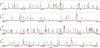 |
Fig. 2 Spectra of spw0 towards core 9 of the AG318.9477−00.1960 clump. The black histogram and its grey shadow are the observational spectrum, and the red curve indicates the LTE fit after taking into account the contribution of all the species (see Table 3 and its complete version in Appendix D.1). The horizontal dashed green line indicates the 5σ ≈ 1.35 K level, with σ being the noise (σ ∼ 0.28 K). Only transitions contributing at ≥ 5σ are labelled. The vertical dashed black lines indicate the position where ν was converged. U labels indicate unidentified transitions. |
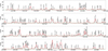 |
Fig. 3 Spectra of spw1 towards core 9 of the AG318.9477−00.1960 clump. The black histogram and its grey shadow are the observational spectrum, and the red curve indicates the LTE fit after taking into account the contribution of all the species (see Table 3 and its complete version in Appendix D.1). The horizontal dashed green line indicates the 5σ ≈ 1.35 K level, with σ being the noise (σ ∼ 0.28 K). Only transitions contributing at ≥5σ are labelled. The vertical dashed black lines indicate the position where ν was converged. U labels indicate unidentified transitions. |
Results of the SLIM fits of the species analysed towards AG318−c9. Only a portion of the table is shown here. The complete table is available in Appendix D.1.
5.2 Comparison with the hot core G31.41+0.31
To place our results in context, we compared the chemical reservoir of AG318−c9 with that of the well-studied HMC G31.41+0.31 (G31 hereafter). G31 is the first core in which GA was detected outside the Galactic centre (Beltrán et al. 2009), and it is one of the first cores in which EG was found (Rivilla et al. 2017). This HMC was also the target of the GUA-POS project, a spectral survey of the entire ALMA band 3 (84.05–115.91 GHz; Mininni et al. 2020). This HMC is located at a DHEL of 3.75 kpc (Immer et al. 2019) with a L = 4.4 × 10⁴ L⊙ (Osorio et al. 2009) and a gas mass M ∼ 70 M⊙ (Cesaroni 2019). By contrast, AG318−c9 is significantly more distant, at a heliocentric distance of ∼10.4 kpc, and its estimated gas mass is M ∼ 120 M⊙ (Coletta et al. 2025). However, this mass is likely an overestimate because it was obtained by assuming a uniform core temperature of 49 K, whereas our Tex maps reveal a temperature gradient in the core with temperatures significantly >49 K (Sect. 6.4), implying a lower total gas mass. Since a core-specific luminosity is unavailable, we estimated it based on the host clump luminosity (2.7 × 10⁵ L⊙), which is fragmented into 19 cores (Coletta et al. 2025). We apportioned the clump luminosity to AG318−c9 by scaling it by the ratio of its peak flux  to the sum of all the core peak fluxes
  , lead ing to Lcore ≈ 1.2 × 10⁵ L⊙, which is almost three times higher than the luminosity of G31. Although we would like to interpret the evolutionary stages of the two HMCs based on their L/M ratios, this approach is subject to significant uncertainties. We note that the interpretation of the evolutionary stage based on global indicators such as the luminosity-to-mass ratio is not straightforward in AG318−c9. The core mass is likely overestimated, while the luminosity is indirectly inferred from the host clump, introducing additional uncertainties. On the other hand, the mass of G31 should be considered as a lower limit (Cesaroni 2019). Additionally, in high-mass star-forming regions, L/M may not provide an unambiguous evolutionary indicator due to the effects of fragmentation, temperature gradients, and internal source structure (Motte et al. 2018).
The GUAPOS survey (Mininni et al. 2020; Colzi et al. 2021; Mininni et al. 2023; Fontani et al. 2024; López-Gallifa et al. 2024, 2025) explored the chemical richness of G31, detecting numerous O- and N-bearing COMs as formamide (HC(O)NH2), methyl isocyanate (CH3NCO), and ethyl iso-cyanide (C2H5NC). A one-to-one comparison of the column density for species detected in the two sources is presented in Fig. 4, where the spectra are extracted over comparable spatial scales (∼6400 au for AG318−c9 and ∼4500 au for G31), indicating that the sampled regions are broadly similar. A clear trend emerges: although G31 has a lower luminosity and mass, the column densities of the species detected towards this HMC are systematically higher than those estimated towards AG318−c9 for most of the species. This discrepancy is particularly pronounced for O-bearing COMs, such as CH3COOH, CH3COCH3, and H2C17O, which show significantly higher N values in G31. Only two species present enhanced N in AG318−c9, which are t − HCOOH, and C18O. N-bearing species also show higher values in G31, but not as high as O-bearing species. S- and Si-bearing species show column densities that are more comparable, clustering closer to the 1:1 correlation line (i.e. within ∼ 1 dex). We found 11 exceptions to the general trend, in which species present enhanced N in AG318−c9: CH3CHO, t-HCOOH, C18O, H2CNH, H15NCO, NH2CN, SO2, SO, 34SO2, SiO, and CH3OCH3.
The observed chemical segregation, characterised by a pronounced excess of O-bearing COMs in G31, strongly suggests a more efficient thermal sublimation of the ice mantles in G31 (Mininni et al. 2023). This implies that G31 is either intrinsically warmer or at a more advanced evolutionary stage than AG318−c9, having had more time to release and accumulate a larger fraction of these species into the gas phase.
N-bearing species have more diverse formation pathways, including active gas-phase chemistry, and require a longer timescale to be synthesised in the cold cloud (Lee et al. 2020). Their abundances are also sensitive to environmental factors such as the UV radiation field, shocks, cosmic-ray ionisation rate, and local N/O elemental ratios. This may explain why their column densities are more comparable between the two sources. Among the exceptions, the higher N of the prebiotic species cyanamide (NH2CN) or the methanimine (H2CNH) in AG318−c9 is particularly noteworthy, suggesting that the physical conditions or precursor availability in AG318−c9 are uniquely favourable for their production. Since D-bearing species are thought to be formed more efficiently, at the low temperatures (< 20K) of the preceding cold core phase, their detection in the hot gas of AG318−c9 implies that they were formed on the ice grains and subsequently sublimated (Caselli & Ceccarelli 2012). However, G31 also presents some of the D-bearing species found in AG318−c9 (V. Rivilla, priv. comm.). This suggests that the two cores share a similar chemical heritage from their cold pre-stellar phase.
The emission of Si- and S-bearing species is usually associated with shocks, as these species would be released from the dust mantles by sputtering. The fact that the column density of these species in both HMCs is comparable suggests that both cores are associated with shocks, likely produced by molecular outflows. For G31, Beltrán et al. (2022) has detected at least six outflows in the core, while for the AG318.9477−00.1960 clump, a preliminary analysis suggests that this core is associated with at least two outflows (M. Benedettini, priv. comm.).
In Fig. 5, we show a comparative histogram of the molecular abundances  for the two sources. We also included the species detected exclusively in G31 and those that are detected in AG318−c9, but were not reported for G31 to date. To ensure a fair comparison, we restricted this selection to species covered by the spectral setups of both surveys. For this reason, we excluded the following molecular species: NS, OCS, NH3, NH2D, N2H+, HCN, CO, CS, CH3CCH, CH3NC, s-C2H5CHO, and 13CO. In addition, a direct comparison with the GUAPOS survey is not yet possible because their full deuterated inventory has not yet been published, and for this reason, DCN, HDCS, CH3OD, CH2DOH, CHD2OH, and DC(O)NH2 are not included in Figs. 4 and 5.
In addition to the enhanced column densities reported above, the comparison based on molecular abundances (Fig. 5) indicates that C2H5CN is comparatively more abundant in AG318−c9. Moreover, a distinct chemical divergence can be noted: G31 features complex N-bearing COMs such as acetamide (CH3CONH2) and methylamine (CH3NH2). The higher N of acetamide is particularly significant because it contains the peptide-like linkage (–NH–C=O), a key component for prebiotic chemistry (Colzi et al. 2021). The molecular inventory of AG318−c9 is distinguished by the presence of O-bearing species that have not been reported in G31 so far, most notably, ethyl formate (C2H5OOCH), along with others such as HOCH2CN. The detection of ethyl formate in AG318−c9, together with its apparent absence in the G31 survey suggests a chemistry dominated by the thermal sublimation of O-rich ice mantles, releasing these O-bearing COMs into the gas phase (Belloche et al. 2009).
This comparison suggests that the two sources might correspond to different evolutionary stages. AG318−c9 might represent a younger HMC, where the chemistry is still dominated by the recent sublimation of ice mantles rich in ester-bearing species. In contrast, G31 appears to be a more evolved environment in which this initial chemical reservoir has likely been processed by warm gas-phase reactions.
Although the overall lower abundances in AG318−c9 are consistent with a less chemically processed source, abundance differences alone do not uniquely constrain the relative evolutionary stage of the two cores. Variations in temperature structure, radiation field, source geometry, or chemical pathways might also contribute to the observed differences (Ossenkopf et al. 2013; Heays et al. 2017). Therefore, the scenario in which AG318−c9 is younger than G31 should be regarded as plausible rather than definitive. These differences indicate distinct chemical evolutionary pathways, although detailed chemical modelling is required to draw firm conclusions.
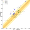 |
Fig. 4 Column density comparison for all common species between AG318−c9 (x-axis) and G31 (y-axis). The solid black line indicates the 1:1 relation. The dark and light orange shaded regions represent deviations within 0.5 dex and 1.0 dex from equality, respectively. |
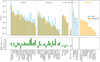 |
Fig. 5 Top: comparison of molecular abundances (X = N/H2) towards G31 (blue bars) and AG318−c9 (orange bars), sorted by molecular groups and by the abundance of AG318−c9 inside each group. The species are grouped on the x-axis according to their detection status. Left: detected in both sources. Middle: detected in G31 alone. The orange triangles represent the corresponding upper limits for AG318−c9. Right: reported in AG318−c9. Bottom: logarithm of the ratio of the abundances of the two sources. HC3N* represents the group composed of HC3N, HC3N (v6 = 1), HC3N (v7 = 1), and HC3N (v7 = 2). |
6 Glycolaldehyde, ethylene glycol, and methyl formate
We focused on the identification of GA, EG, and MF emission towards AG318−c9, paying particular attention to line-blending effects that might affect their detection. GA stands out as a key prebiotic species, being the simplest sugar-like monosaccharide molecule that plays a fundamental role in sugar-formation pathways, leading to the formation of essential biomolecules such as glyceraldehyde and ribose, the backbone of nucleic acids. GA has been detected in different star-forming regions in the ISM, including the first detection in Sgr B2(N) in the Galactic centre (Hollis et al. 2000), the HMC G31.41+0.31 (Beltrán et al. 2009), and the solar-type protostar IRAS 16293-2422 (Jørgensen et al. 2012).
The heavy COM EG, with ten atoms, and the fully reduced form of GA where the aldehyde group has been reduced to an alcohol, although not directly prebiotic, is chemically linked to GA, and they may both share the same formation pathways in the ISM (Sorrell 2001; Fedoseev et al. 2015; Coutens et al. 2018; Garrod et al. 2022). EG was first found in the ISM towards the Galactic centre (Hollis et al. 2002) in HMCs such as G31.41 + 0.31 (Rivilla et al. 2017) or G34.3 + 0.1 (Brouillet et al. 2015) and in hot corinos such as NGC 1333-IRAS 2A (Maury et al. 2014).
Finally, MF, although not chemically linked through the same formation pathways, can offer complementary constraints on the chemistry of GA and EG. All three species are expected to trace similar physical conditions (Simons et al. 2020).
6.1 Glycolaldehyde
In Fig. 6 we show all 19 transitions of GA, clearly above S/N ≥ 5. The transition 202,18 → 193,17 is the brightest and has the highest opacity (τ = 0.061), confirming that all the GA transitions are optically thin. Unlike for EG and MF (Sects. 6.2 and 6.3), in the available ALMAGAL frequency coverage, there are few unblended transitions of GA. There are three unblended transitions: 95,5 → 84,4 at 217626.13 MHz, 314,27 → 313,28 at 217271.61 MHz, and 203,17 → 194,16 at 218260.59 MHz. Most of the blending of GA is with CH3COCH3,  , CH3OCH3, and CH3NCO transitions, whose contribution is included in the global red fit in Fig. 6, and it explains the remaining features of the observed spectrum. The fitted transitions span a broad range of energies (Eup = 26–316 cm−1 or 37–450 K).
Although SLIM converged to a solution for GA without the need to fix any parameter, we fixed the FWHM to 4.0 km s−1, as the line width obtained from the unconstrained fit might be visually refined to match the observed spectra better. The resulting fit of the detected transitions of GA indicates Tex = 168 ± 13 K, N = (1.45 ± 0.12) × 1016 cm−2 and V = −36.89 ± 0.1 km s−1.
6.2 Ethylene glycol
Ethylene glycol is a heavy COM and the fully reduced alcohol form of GA. The presence of both species, which are thought to be chemically linked through common formation pathways (Coutens et al. 2018; Simons et al. 2020; Garrod et al. 2022), confirms the complexity of the chemistry in AG318−c9. EG can adopt different conformations because torsions around its C–C bond and its two C–O bonds lead to four forms with an anti-arrangement (a-EG) of the hydroxyl groups (–OH), and six with a gauche-arrangement (g-EG) (Kazerouni et al. 1997; Rivilla et al. 2017). We focused on the a-EG conformer because it shows a significantly larger number of transitions within the ALMA-GAL spectral setup compared to the g-EG conformer. The latter shows many blended lines, and the few unblended transitions have similar energies, Eup ≈ 130 K, so that it is difficult to properly constrain the physical parameters.
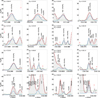
Figure 7 shows selected lines corresponding to a-EG, eight of which are unblended and strong. Other transitions are more blended, mainly with MF, CH3NCO, HNCO, HN13CO, C2H5OH, and CHD2OH. The 241,24 → 231,23 transition at 217450 MHz is the brightest and the most optically thick with τ = 0.046. To fit the EG emission, we took 37 different transitions into account, which span a range of energies of Eup = 79–389 cm−1 or 114–580 K. Fig. 7 shows that the LTE fit, with the joint contribution of all blending species, is able to properly explain the observed emission.
For a-EG, SLIM converged to a solution for a-EG without the need to fix any parameters. The resulting fit of the detected transitions of a-EG indicates Tex = 240 ± 30 K, N = (5.1 ± 0.6) × 1016 cm−2, FWHM = 6.19 ± 0.19 km s−1, and V = −35.9 ± 0.08 km s−1.
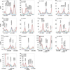 |
Fig. 6 Selection of GA transitions observed and fit (see Sect. 6.1). The black histogram and its grey shadow are the observational spectrum, and the red curve is the cumulative LTE fit considering all detected species. The blue curve is the fit of the individual transitions. The horizontal dashed green line indicates the 5σ level, corresponding to ∼1.35 K. Only transitions contributing at ≥5σ are labelled. The plots are sorted by decreasing intensity of the GA transitions (blue line). The upper left corner of each panel indicates the EUP of the corresponding GA transition. When multiple GA transitions are shown in the same panel, the EUP values are listed from top to bottom following the left-to-right order of the transitions. |
6.3 Methyl formate
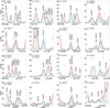
Methyl formate shows the highest number of clean transitions of the three COMs, with a total of 14 unblended transitions. In Fig. 8, we show selected lines corresponding to MF. To fit the MF emission, we took a total of 41 transitions into account (see Appendix A), with 173,14 → 163,13 at 218297.89 MHz being the brightest. The same transition also has the largest τ = 0.185, being the transition with highest opacity among all the fitted transitions of EG, GA, and MF. In any case, we can still consider all MF transitions as optically thin. The fitted MF transitions cover a wide energy range Eup = 69–318 cm−1 or 100–457 K.
The estimated excitation temperature, Tex = 167 ± 3 K, is consistent with that derived for EG and GA. The column density is one order of magnitude higher N = (2.2 ± 0.4) × 1017 cm−2 than those of EG and GA, which indicates that MF is more abundant, as already observed in other works (Hollis et al. 2001; Mininni et al. 2020). In the case of MF, we did not fix any parameter. We obtained a value for the FWHM = 5.59 ± 0.08 km s−1 and V = −35.22 ± 0.04 km s−1, which are similar to those of EG and GA.
6.4 Integrated intensity, Tex, and N maps of EG, GA, and MF
A key aspect of our analysis is to understand how EG, GA, and MF trace the physical environment of AG318−c9. To this end, we used MADCUBA to compute their integrated intensity (moment 0), N and Tex maps (Appendix B), together with radial profiles of N and Tex obtained by averaging the values within annuli of 0.″1. The resulting maps and profiles are presented in Figs. 9–11, and the corresponding relative uncertainty maps are shown in Appendix B.1.
To generate the maps, we initially attempted to use the same transitions as we adopted to derive the physical parameters presented in Sect. 5.1. However, for EG and GA, a reduced set of transitions was selected, prioritising the least blended transitions while preserving a broad energy coverage. This choice was necessary to ensure convergence of the fits, particularly in the outer core regions with a lower S/N, where the inclusion of blended transitions prevented reliable solutions. The transitions used to produce the maps are listed in Appendix B.2. For EG, the selected transitions cover the same energy range as used in the global fit (Eup = 114–580 K), while for GA, they span a similar range (Eup = 37–410 K).
The moment 0 maps shown in Fig. 9 were constructed using representative transitions for each molecule: the 3510,26 → 359,27 transition at 220.055 GHz for GA (Eup = 410 K), the 241,24 → 231,23 transition at 217.45 GHz for EG (Eup = 117 K), and the 173,14 → 163,13 transition at 218.298 GHz for MF (Eup = 100 K). While the EG and MF moment 0 maps were generated with comparable upper-level energies, the GA map relied on a significantly higher Eup transition. This difference requires caution when interpreting relative spatial extents based solely on moment 0 emission. Although the moment 0 maps were required to automate the generation of the N and Tex maps, they were not used to derive these quantities directly. Instead, they were used solely to estimate the noise level, which was then applied to assess the reliability of the pixel-by-pixel spectral fits and to exclude solutions below a 3σ threshold (Appendix B). The N and Tex maps are therefore based on multi-transition fits and are not biased by the specific energy of the moment 0 transition.
To generate N and Tex maps, only the target species was considered in each case, without considering the contribution of other molecules (Appendix B). As a result, the core-averaged physical parameters reported in Tables 3 and D.1, which account for all detected species, are more robust. Nevertheless, the values derived from the maps are consistent with the core-averaged quantities.
Of the three species, MF is most spatially extended. Its emission closely follows the dust continuum emission and peaks near the continuum maximum (Fig. 9). The N(MF) map (Fig. 10) reveals a very similar morphology, with a clear column density gradient ranging from ∼1016 cm−2 in the outer regions to ∼3.16× 1017 cm−2 near the continuum peak, corresponding to the highest N among the three COMs. The gradient is clearly reflected in the radial profile (Fig. 11), which decreases steadily from the core centre towards larger radii. The Tex(MF) map (Fig. 10) shows a robust temperature gradient, rising from ∼100 K in the outer parts of the core up to ∼250 K towards the centre. The radial profile presents a more rapid temperature increase inward of 0.″8. This combination of large spatial extent and wide Tex dynamic range confirms MF as an excellent tracer of the gas temperature and its gradients in HMCs (e.g. Beltrán et al. 2018). These temperatures are consistent with the high rotational temperatures (120–300 K) expected in hot cores (Herbst & van Dishoeck 2009) and typical Tex ∼ 150 K estimates Cesaroni 2005, Bisschop et al. 2007; Rivilla et al. 2017. Because MF has the most unblended transitions, its Tex map has the lowest relative error  , which increases only in the outer regions with a lower S/N (Appendix B.1).
The distribution of EG is more compact. Its integrated-intensity and column density maps (Figs. 9 and 10) are more concentrated towards the inner core. The N(EG) increases from ∼1015 cm−2 at the edges to ∼5 × 1016 cm−2 towards the centre. The relative errors for N(EG) increase slightly in the centre of the emission (Fig. B.1). The Tex(EG) map (Fig. 10) does not exhibit a well-defined peak as clearly as for MF. For clarity, the map is truncated at a radius of 0.″9 beyond which the uncertainties become too large for a reliable interpretation. Within this radius, the highest Tex values are found within the core, coinciding with the region of strongest dust continuum emission. Overall, the temperature distribution appears to be relatively uniform throughout the inner region where EG emission is detected, with a relative error of ∼30% (Fig. B.2). This behaviour might partly reflect the greater difficulty in constraining the fits due to fewer unblended lines, as reflected in the higher relative error, which increases considerably in the outer colder region. Nevertheless, the radial profile clearly decreases in temperature from ∼170 K to ∼80 K with increasing distance from the core centre, although the profile appears to be less steep in the innermost regions.
The most compact species is GA, with emission confined to the innermost region of the core, close to the continuum peak. The N(GA) and Tex(GA) maps peak centrally, with column densities ranging from ∼2 × 1016 cm−2 to ∼4 × 1016 cm−2 and an excitation temperature between ∼130 K to ∼160 K. The two map fits have a relative error of ∼10–15% (Appendix B.1). Over the radial range in which EG and GA are detected, the N gradient is comparable to that estimated in EG.
To evaluate whether the different spatial extents of MF, EG, and GA are driven by sensitivity limitations or reflect intrinsic chemical differentiation, we estimated the column density corresponding to a 5σ detection threshold (∼1.35 K) for each molecule with MADCUBA. For MF and EG, the 5σ limits (N ∼ 1016 cm−2 and N ∼ 2.5 × 1015 cm−2, respectively) closely match the minimum column densities reached by their radial profiles, indicating that the apparent truncation is largely driven by sensitivity. In contrast, the 5σ threshold for GA is N(GA) ≈ 2 × 1015 cm−2, whereas the GA radial profile only extends to N(GA) ≈ 1.6 × 1016 cm−2, almost one order of magnitude. This might suggest that the lack of detectable GA emission beyond the innermost regions of the core is not limited by sensitivity, but instead reflects its intrinsically compact distribution.
The compact emission of EG and GA suggests that they are excellent candidates for tracing the innermost high-density regions of the core. Due to their optically thin transitions, they might also be used to probe the kinematics within these regions. Furthermore, the fact that EG and GA are only detected in the warm inner region, unlike the more extended MF, might imply that a specific temperature threshold must be reached to sublimate them from the icy dust grains. This observation strongly supports a shared grain-surface formation pathway, consistent with models of dust-grain chemistry (e.g. Fedoseev et al. 2015; Simons et al. 2020; Garrod et al. 2022).
However, the innermost region must be interpreted with caution due to observational effects. At radii comparable to or smaller than the beam size (∼0.″21), the observed brightness temperature might be affected by beam dilution. In addition, dust opacity might become non-negligible towards the core centre, potentially attenuating line emission from the deepest layers. These effects might result in an underestimation of the true column densities and excitation temperatures in the central region, particularly for compact species such as EG and GA. Moreover, as shown in Fig. 11, the emission of the three species extends beyond the beam size, and therefore, it is expected to be hardly affected by beam dilution.
The observed spatial differentiation among the three species suggests that their distributions are not governed solely by thermal desorption, but also by their formation pathways and ice chemistry. MF, with a lower binding energy (∼4000 K; desorption at ∼100–120 K), is expected to be more extended and associated with CO-rich outer regions, whereas GA has a higher binding energy (∼5900 K; ∼140–190 K) and is therefore expected to trace warmer and denser regions, consistent with its more compact emission (Öberg et al. 2009). EG, with an even higher binding energy (∼7500 K; ∼150–180 K), does not show a correspondingly more compact distribution, suggesting that its spatial extent cannot be explained by desorption alone. Instead, its distribution might reflect efficient formation during the warm-up phase, such as via CH2OH recombination and chemical stability once released into the gas phase (Öberg et al. 2009; Fedoseev et al. 2015). Overall, this chemical differentiation supports a scenario in which the temperature gradients and the initial ice composition can play a key role in shaping the spatial distribution of COMs (Garrod et al. 2008).
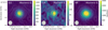 |
Fig. 9 Integrated-intensity maps for EG (left), GA (middle), and MF (right). The white contours correspond to the continuum emission at 5σ, 10σ, 20σ, 30σ, 60σ, 90σ, 180σ, 220σ, and 260σ with σ = 0.28 mJy beam−1, and the red cross shows its peak position. The red ellipses surrounded by white show the location and size of the dust continuum core AG318−c9 as estimated by Coletta et al. (2025). The hatched ellipse shown in the bottom left corner represents the synthesised beam of the interferometer. |
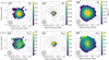 |
Fig. 10 Column density (N) maps (top row) and excitation temperature (Tex) maps (bottom row) derived for EG (left), GA (middle), and MF (right). The corresponding relative errors are shown in Appendix B.1. The black contours correspond to the continuum emission at 5σ, 10σ, 20σ, 30σ, 60σ, 90σ, 180σ, 220σ, and 260σ with σ = 0.28 mJy beam−1, and the red cross shows its peak position. The red ellipses surrounded by white show the location and size of the dust continuum core AG318−c9 as estimated by Coletta et al. (2025). The hatched ellipse shown in the bottom left corner represents the synthesised beam of the interferometer. |
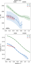 |
Fig. 11 Radial profiles derived from the column density (N; top) and excitation temperature (Tex; bottom) maps. The blue, red, and green curves correspond to EG, GA, and MF, respectively. The shaded areas indicate the measurement uncertainties (see Appendix B.1). The bar in the lower left corner indicates the radius corresponding to the geometric mean of the synthetic beam. |
7 Conclusions
We presented a comprehensive analysis of the chemical reservoir of the AG318.9477−0.1960 clump core 9 using data from the ALMAGAL project and a frequency range of ∼217–221 GHz. Throughout the ∼ 4 GHz setup, we identified 65 species, of which 44 are O-bearing species, 28 are N-bearing, 8 are S-bearing, and 2 are Si-bearing. Thirty-three of these species are COMs. The fact that most of the detections are O-bearing molecules suggests an efficient thermal sublimation of the ice mantles into the gas phase. For all the detected species, we derived their physical parameters and abundances with respect to H2.
This spectral analysis allowed us to characterise weak and blended species, such as the three COMs of interest: EG, GA, and MF. For EG, we covered an EUP range of 114–580 K and detected 8 unblended transitions. We found that the species that are more strongly blended with EG are MF, CH3NCO, HNCO, HN13CO, C2H5OH, and CHD2OH. For GA, we traced transitions with EUP = 37–450 K including 3 unblended lines. The main blending species are CH3COCH3,  , CH3OCH3, and CH3NCO. Finally, MF exhibited transitions with EUP = 100–457 K and 14 unblended lines, making it the species least affected by blending. All three species trace warm and dense gas, although they probe distinct thermal components. EG traces the warmest material, with a Tex of ∼240 K. GA and MF trace slightly cooler gas, with Tex ∼168 K and ∼167 K, respectively. Regarding N and abundance, MF has a column density of ∼2 × 1017 cm−2 and is clearly the most abundant species, with X ∼ 3 × 10⁻⁸. This abundance is significantly higher than that of EG and GA, which have abundances of ∼7 × 10⁻⁹ and ∼2 × 10⁻⁹, and N of ∼5 × 1016 cm−2 and ∼1.5 × 1016 cm−2, respectively.
The chemical comparison with the chemically rich HMC G31.41+0.31 indicated that this core shows systematically higher column densities than AG318−c9 for O- and N-bearing COMs. This suggests that G31 is either intrinsically warmer or at a more advanced evolutionary stage than AG318−c9, having experienced more efficient thermal sublimation of its ice mantles. This comparison also revealed a chemical differentiation between these families, with a stronger enhancement of O-bearing species in G31, while N-bearing species showed a more moderate contrast between the two sources. Conversely, S-bearing species are more comparable between the two sources. Notably, AG318−c9 shows a significant overabundance of the prebiotic molecules NH2CN and H2CNH, which indicates specific physical conditions or precursor availability for its formation.
Our analysis of the Tex and N maps for EG, GA, and MF within AG318−c9 revealed distinct morphologies. The emission of the three species extends beyond the beam size and is therefore not significantly affected by beam dilution. However, observational effects, in particular, dust opacity, might still lead to underestimated column densities and excitation temperatures in the innermost region. MF shows significantly higher column densities (N ≈ 3 × 1017 cm−2) and a spatially extended distribution, robustly tracing the thermal structure of the core over a broad temperature range (Tex ∼ 100–250 K). In sharp contrast, EG and GA are compact and confined to the innermost core region, with GA being particularly compact. They both exhibit similar lower column densities (N ≈ 4 × 1016 cm−2). Their restricted distribution indicates that they only trace the warmest densest gas, implying a high sublimation temperature threshold. This might support a shared grain-surface formation pathway.
As a methodological output of this work, we developed two MADCUBA scripts that will be used for future molecular analysis studies within the ALMAGAL survey. Work is now underway on a complete study of EG, GA, and MF in all ALMAGAL cores to understand the correlations between these COMs, the physical conditions that lead to their formation, and their possible chemical pathways.
Data availability
The scripts used for the automated line identification and map generation, as well as the complete table of molecular transitions used for the MADCUBA fits of the molecular emission towards AG318−c9 (see Tables 2, 3, and D.1) are available at: https://github.com/JofreAllande/ALMAGAL/.
Acknowledgements
We thank the anonymous referee for the useful comments. The table of molecular transitions were made thanks to the Python library RichValues6 created by Andrés Megías. J.A. acknowledges the SKA PhD fellowship “Astrochemistry of prebiotic molecules in high-mass star-forming regions in preparation of the SKA observations” offered by INAF. C.Y.L. acknowledges financial support through the INAF Large Grant “The role of MAGnetic fields in MAssive star formation” (MAGMA). R.S.K acknowledges financial support from the ERC via Synergy Grant “ECOGAL” (project ID 855130) and from the German Excellence Strategy via the Heidelberg Cluster “STRUCTURES” (EXC 2181 – 390900948). In addition R.S.K. is grateful for funding from the German Ministry for Economic Affairs and Climate Action in project “MAINN” (funding ID 50OO2206), and from DFG and ANR for project “STARCLUSTERS” (funding ID KL 1358/22-1). L.C. acknowledges support from the grant PID2022-136814NB-I00 by the Spanish Ministry of Science, Innovation and Universities/State Agency of Research MICI-U/AEI/10.13039/501100011033 and by ERDF, UE. The project that gave rise to these results received the support of a fellowship from the “la Caixa” Foundation (ID 100010434). The fellowship code is LCF/BQ/PR25/12110012. L.B. gratefully acknowledges support by the ANID BASAL project FB210003. C.M. and the INAF-IAPS team acknowledge funding from the European Research Council (ERC) under the European Union’s Horizon 2020 program through the ECOGAL Synergy grant (ID 855130). C.M. acknowledges funding from INAF Mini Grants RSN2 2024 "Zodyac" CUP C83C25000340005. R.K. acknowledges financial support via the Heisenberg Research Grant funded by the Deutsche Forschungs-gemeinschaft (DFG, German Research Foundation) under grant no. KU 2849/9, project no. 445783058. A.S.-M. acknowledges support from the RyC2021-032892-I grant funded by MCIN/AEI/10.13039/501100011033 and by the European Union ‘Next GenerationEU’/PRTR, as well as the program Unidad de Excelencia María de Maeztu CEX2020-001058-M, and support from the PID2020-117710GB-I00 (MCI-AEI-FEDER, UE). A.L-G. acknowledges support from the grant PID2022-136814NB-I00 by the Spanish Ministry of Science, Innovation and Universities/State Agency of Research MICIU/AEI/10.13039/501100011033 and by ERDF, UE; and from the Consejo Superior de Investigaciones Científicas (CSIC) and the Centro de Astrobiología (CAB) through the project 20225AT015 (Proyectos intramurales especiales del CSIC). The National Radio Astronomy Observatory is a facility of the National Science Foundation operated under cooperative agreement by Associated Universities, Inc. Part of this research was carried out at the Jet Propulsion Laboratory, California Institute of Technology, under a contract with the National Aeronautics and Space Administration (80NM0018D0004).
References
- Baek, G., Lee, J.-E., Hirota, T., Kim, K.-T., & Kyoung Kim, M. 2022, ApJ, 939, 84 [NASA ADS] [CrossRef] [Google Scholar]
- Balucani, N., Ceccarelli, C., & Taquet, V. 2015, MNRAS, 449, L16 [Google Scholar]
- Belloche, A. 2017, Proc. IAU, 13, 383 [Google Scholar]
- Belloche, A., Garrod, R. T., Müller, H. S. P., et al. 2009, A&A, 499, 215 [NASA ADS] [CrossRef] [EDP Sciences] [Google Scholar]
- Belloche, A., Müller, H. S. P., Menten, K. M., Schilke, P., & Comito, C. 2013, A&A, 559, A47 [NASA ADS] [CrossRef] [EDP Sciences] [Google Scholar]
- Belloche, A., Garrod, R. T., Müller, H. S. P., et al. 2025, A&A, 698, A143 [NASA ADS] [CrossRef] [EDP Sciences] [Google Scholar]
- Beltrán, M. T., Cesaroni, R., Neri, R., et al. 2005, A&A, 435, 901 [Google Scholar]
- Beltrán, M. T., Codella, C., Viti, S., Neri, R., & Cesaroni, R. 2009, ApJ, 690, L93 [Google Scholar]
- Beltrán, M. T., Cesaroni, R., Rivilla, V. M., et al. 2018, A&A, 615, A141 [Google Scholar]
- Beltrán, M. T., Rivilla, V. M., Kumar, M. S. N., Cesaroni, R., & Galli, D. 2022, A&A, 660, L4 [NASA ADS] [CrossRef] [EDP Sciences] [Google Scholar]
- Bisschop, S. E., Jørgensen, J. K., van Dishoeck, E. F., & de Wachter, E. B. M. 2007, A&A, 465, 913 [NASA ADS] [CrossRef] [EDP Sciences] [Google Scholar]
- Boogert, A. C. A., Gerakines, P. A., & Whittet, D. C. B. 2015, ARA&A, 53, 541 [Google Scholar]
- Brouillet, N., Despois, D., Lu, X. H., et al. 2015, A&A, 576, A129 [NASA ADS] [CrossRef] [EDP Sciences] [Google Scholar]
- Caselli, P., & Ceccarelli, C. 2012, A&A Rev., 20, 56 [NASA ADS] [Google Scholar]
- Ceccarelli, C., Codella, C., Balucani, N., et al. 2022, arXiv e-prints [arXiv:2206.13270] [Google Scholar]
- Cesaroni, R. 2005, in IAU Symposium, 227, Massive Star Birth: A Crossroads of Astrophysics, eds. R. Cesaroni, M. Felli, E. Churchwell, & M. Walmsley, 59 [NASA ADS] [Google Scholar]
- Cesaroni, R. 2019, A&A, 631, A65 [NASA ADS] [CrossRef] [EDP Sciences] [Google Scholar]
- Cesaroni, R., Beltrán, M. T., Zhang, Q., Beuther, H., & Fallscheer, C. 2011, A&A, 533, A73 [NASA ADS] [CrossRef] [EDP Sciences] [Google Scholar]
- Chen, Y., van Gelder, M. L., Nazari, P., et al. 2023, A&A, 678, A137 [NASA ADS] [CrossRef] [EDP Sciences] [Google Scholar]
- Coletta, A., Fontani, F., Rivilla, V., et al. 2020, A&A, 641, A54 [NASA ADS] [CrossRef] [EDP Sciences] [Google Scholar]
- Coletta, A., Molinari, S., Schisano, E., et al. 2025, A&A, 696, A151 [NASA ADS] [CrossRef] [EDP Sciences] [Google Scholar]
- Colzi, L., Rivilla, V. M., Beltrán, M. T., et al. 2021, A&A, 653, A129 [NASA ADS] [CrossRef] [EDP Sciences] [Google Scholar]
- Coutens, A., Viti, S., Rawlings, J. M. C., et al. 2018, MNRAS, 475, 2016 [NASA ADS] [CrossRef] [Google Scholar]
- De Buizer, J. M. 2003, MNRAS, 341, 277 [CrossRef] [Google Scholar]
- De Buizer, J. M., Redman, R. O., Longmore, S. N., Caswell, J., & Feldman, P. A. 2009, A&A, 493, 127 [NASA ADS] [CrossRef] [EDP Sciences] [Google Scholar]
- Elia, D., Strafella, F., Dib, S., et al. 2018, MNRAS, 481, 509 [Google Scholar]
- Elia, D., Merello, M., Molinari, S., et al. 2021, MNRAS, 504, 2742 [NASA ADS] [CrossRef] [Google Scholar]
- Elia, D., Coletta, A., Molinari, S., et al. 2026, A&A, 705, A100 [NASA ADS] [CrossRef] [EDP Sciences] [Google Scholar]
- Endres, C. P., Schlemmer, S., Schilke, P., Stutzki, J., & Müller, H. S. P. 2016, J. Mol. Spectrosc., 327, 95 [NASA ADS] [CrossRef] [Google Scholar]
- Escoffier, R. P., Comoretto, G., Webber, J. C., et al. 2007, A&A, 462, 801 [NASA ADS] [CrossRef] [EDP Sciences] [Google Scholar]
- Fedoseev, G., Cuppen, H. M., Ioppolo, S., Lamberts, T., & Linnartz, H. 2015, MNRAS, 448, 1288 [NASA ADS] [CrossRef] [Google Scholar]
- Fontani, F., Mininni, C., Beltrán, M. T., et al. 2024, A&A, 682, A74 [NASA ADS] [CrossRef] [EDP Sciences] [Google Scholar]
- Fuchs, G. W., Cuppen, H. M., Ioppolo, S., et al. 2009, A&A, 505, 629 [NASA ADS] [CrossRef] [EDP Sciences] [Google Scholar]
- Garrod, R. T., Widicus Weaver, S. L., & Herbst, E. 2008, ApJ, 682, 283 [Google Scholar]
- Garrod, R. T., Jin, M., Matis, K. A., et al. 2022, ApJS, 259, 1 [NASA ADS] [CrossRef] [Google Scholar]
- Heays, A. N., Bosman, A. D., & van Dishoeck, E. F. 2017, A&A, 602, A105 [NASA ADS] [CrossRef] [EDP Sciences] [Google Scholar]
- Herbst, E., & van Dishoeck, E. F. 2009, ARA&A, 47, 427 [Google Scholar]
- Hoare, M. G., Lumsden, S. L., Oudmaijer, R. D., et al. 2005, in IAU Symposium, 227, Massive Star Birth: A Crossroads of Astrophysics, eds. R. Cesaroni, M. Felli, E. Churchwell, & M. Walmsley, 370 [NASA ADS] [Google Scholar]
- Hollis, J. M., Lovas, F. J., & Jewell, P. R. 2000, ApJ, 540, L107 [Google Scholar]
- Hollis, J. M., Vogel, S. N., Snyder, L. E., Jewell, P. R., & Lovas, F. J. 2001, ApJ, 554, L81 [Google Scholar]
- Hollis, J. M., Lovas, F. J., Jewell, P. R., & Coudert, L. H. 2002, ApJ, 571, L59 [NASA ADS] [CrossRef] [Google Scholar]
- Iguchi, S., Morita, K.-I., Sugimoto, M., et al. 2009, PASJ, 61, 1 [NASA ADS] [CrossRef] [Google Scholar]
- Immer, K., Li, J., Quiroga-Nuñez, L. H., et al. 2019, A&A, 632, A123 [NASA ADS] [CrossRef] [EDP Sciences] [Google Scholar]
- Jørgensen, J. K., Favre, C., Bisschop, S. E., et al. 2012, ApJ, 757, L4 [Google Scholar]
- Jørgensen, J. K., van der Wiel, M. H. D., Coutens, A., et al. 2016, A&A, 595, A117 [Google Scholar]
- Jørgensen, J. K., Belloche, A., & Garrod, R. T. 2020, ARA&A, 58, 727 [Google Scholar]
- Kazerouni, M. R., Hedberg, L., & Hedberg, K. 1997, J. Am. Chem. Soc., 119, 8324 [Google Scholar]
- Kerr, A. R., Pan, S. K., Lauria, E. F., et al. 2004, in Fifteenth International Symposium on Space Terahertz Technology, ed. G. Narayanan, 55 [Google Scholar]
- Lee, J.-K., Walsh, A., Burton, M., & Ashley, M. 2001, MNRAS, 324, 1102 [NASA ADS] [CrossRef] [Google Scholar]
- Lee, S., Lee, J.-E., Aikawa, Y., Herczeg, G., & Johnstone, D. 2020, ApJ, 889, 20 [NASA ADS] [CrossRef] [Google Scholar]
- Levenberg, K. 1944, Q. Appl. Math., 2, 164 [Google Scholar]
- Linnartz, H., Ioppolo, S., & Fedoseev, G. 2015, arXiv e-prints [arXiv:1507.02729] [Google Scholar]
- López-Gallifa, Á., Rivilla, V. M., Beltrán, M. T., et al. 2024, MNRAS, 529, 3244 [CrossRef] [Google Scholar]
- López-Gallifa, Á., Rivilla, V. M., Beltrán, M. T., et al. 2025, A&A, 704, A288 [NASA ADS] [CrossRef] [EDP Sciences] [Google Scholar]
- Lumsden, S. L., Hoare, M. G., Urquhart, J. S., et al. 2013, ApJS, 208, 11 [Google Scholar]
- Marquardt, D. W. 1963, jstor, 11, 431 [Google Scholar]
- Martín, S., Martín-Pintado, J., Blanco-Sánchez, C., et al. 2019, A&A, 631, A159 [Google Scholar]
- Maury, A. J., Belloche, A., André, P., et al. 2014, A&A, 563, L2 [NASA ADS] [CrossRef] [EDP Sciences] [Google Scholar]
- Mininni, C., Beltrán, M. T., Rivilla, V. M., et al. 2020, A&A, 644, A84 [NASA ADS] [CrossRef] [EDP Sciences] [Google Scholar]
- Mininni, C., Beltrán, M. T., Colzi, L., et al. 2023, A&A, 677, A15 [NASA ADS] [CrossRef] [EDP Sciences] [Google Scholar]
- Mininni, C., Molinari, S., Soler, J. D., et al. 2025, A&A, 699, A34 [NASA ADS] [CrossRef] [EDP Sciences] [Google Scholar]
- Molinari, S., Schisano, E., Faustini, F., et al. 2011, A&A, 530, A133 [NASA ADS] [CrossRef] [EDP Sciences] [Google Scholar]
- Molinari, S., Schisano, E., Elia, D., et al. 2016, A&A, 591, A149 [NASA ADS] [CrossRef] [EDP Sciences] [Google Scholar]
- Molinari, S., Schilke, P., Battersby, C., et al. 2025, A&A, 696, A149 [NASA ADS] [CrossRef] [EDP Sciences] [Google Scholar]
- Motte, F., Bontemps, S., & Louvet, F. 2018, ARA&A, 56, 41 [Google Scholar]
- Müller, H. S. P. 2025, Molecules in Space [Google Scholar]
- Müller, H. S. P., Thorwirth, S., Roth, D. A., & Winnewisser, G. 2001, A&A, 370, L49 [Google Scholar]
- Müller, H. S. P., Schlöder, F., Stutzki, J., & Winnewisser, G. 2005, J. Mol. Struct., 742, 215 [Google Scholar]
- Nazari, P. 2026, Life Sci. Space Res., 49, 4 [Google Scholar]
- Öberg, K. I. 2016, Chem. Rev., 116, 9631 [Google Scholar]
- Öberg, K. I., Garrod, R. T., van Dishoeck, E. F., & Linnartz, H. 2009, A&A, 504, 891 [NASA ADS] [CrossRef] [EDP Sciences] [Google Scholar]
- Osorio, M., Anglada, G., Lizano, S., & D’Alessio, P. 2009, ApJ, 694, 29 [Google Scholar]
- Ossenkopf, V., Röllig, M., Neufeld, D. A., et al. 2013, A&A, 550, A57 [NASA ADS] [CrossRef] [EDP Sciences] [Google Scholar]
- Padovani, M., Ivlev, A. V., Galli, D., et al. 2020, Space Sci. Rev., 216, 29 [CrossRef] [Google Scholar]
- Pickett, H. M., Poynter, R. L., Cohen, E. A., et al. 1998, J. Quant. Spec. Radiat. Transf., 60, 883 [Google Scholar]
- Purser, S. J. D., Lumsden, S. L., Hoare, M. G., et al. 2016, MNRAS, 460, 1039 [NASA ADS] [CrossRef] [Google Scholar]
- Rivilla, V. M., Beltrán, M. T., Cesaroni, R., et al. 2017, A&A, 598, A59 [NASA ADS] [CrossRef] [EDP Sciences] [Google Scholar]
- Sánchez-Monge, Á., Brogan, C. L., Hunter, T. R., et al. 2025, A&A, 696, A150 [Google Scholar]
- Santos, J. C., Chuang, K.-J., Lamberts, T., et al. 2022, ApJ, 931, L33 [NASA ADS] [CrossRef] [Google Scholar]
- Schisano, E., Molinari, S., Coletta, A., et al. 2026, A&A, 707, A221 [NASA ADS] [CrossRef] [EDP Sciences] [Google Scholar]
- Simons, M. A. J., Lamberts, T., & Cuppen, H. M. 2020, A&A, 634, A52 [NASA ADS] [CrossRef] [EDP Sciences] [Google Scholar]
- Skouteris, D., Balucani, N., Ceccarelli, C., et al. 2018, ApJ, 854, 135 [NASA ADS] [CrossRef] [Google Scholar]
- Sorrell, W. H. 2001, ApJ, 555, L129 Tielens, A. G. G. M. 2013, RMP, 85, 1021 [Google Scholar]
- Urquhart, J. S., Busfield, A. L., Hoare, M. G., et al. 2007, A&A, 461, 11 [NASA ADS] [CrossRef] [EDP Sciences] [Google Scholar]
- Voronkov, M. A., Caswell, J. L., Ellingsen, S. P., Green, J. A., & Breen, S. L. 2014, MNRAS, 439, 2584 [NASA ADS] [CrossRef] [Google Scholar]
- Wallace, J., Kolz, T., Battersby, C., et al. 2026, ApJ, 998, 302 [Google Scholar]
- Watanabe, N., & Kouchi, A. 2002, ApJ, 571, L173 [Google Scholar]
- Wells, M. R. A., Beuther, H., Molinari, S., et al. 2024, A&A, 690, A185 [NASA ADS] [CrossRef] [EDP Sciences] [Google Scholar]
- Wootten, A., & Thompson, A. R. 2009, IEEE Proc., 97, 1463 [NASA ADS] [CrossRef] [Google Scholar]
- Yan, Y. T., Zhang, J. S., Henkel, C., et al. 2019, ApJ, 877, 154 [Google Scholar]
- Yan, Y. T., Henkel, C., Kobayashi, C., et al. 2023, A&A, 670, A98 [NASA ADS] [CrossRef] [EDP Sciences] [Google Scholar]
The complete table of molecular transitions used for the MADCUBA fits is available at https://github.com/JofreAllande/ALMAGAL/
Appendix A Automatization with MADCUBA
We developed a MADCUBA macro to automate line identification across the ALMAGAL sample. Molecular species identified toward AG318−c9 using the detailed line identification described in Sect. 4.2 were added to the SLIM module using the CDMS7 (Müller et al. 2001, 2005; Endres et al. 2016) or the JPL8 (Pickett et al. 1998) catalogues. As previously mentioned, for each species only sufficiently strong (S/N ≥ 5) and partially unblended transitions were selected, ensuring that AUT-OFIT operates on high-quality lines and minimising potential errors from blended or contaminated transitions. In future studies where the entire ALMAGAL sample will be analysed and chemically poorer sources will be included, the presence of species detected in AG318−c9 will not pose a problem, since AUTOFIT will not converge for species absent in the observed spectra and will not affect the fitting of other species.
SLIM requires an initial input of N, Tex, V, FWHM, and θs for each species to run AUTOFIT. If these initial values are absent or far from realistic estimates, the programme does not converge. For AG318−c9, we assumed as initial guesses V = −34.4 km s−1, which is the systemic velocity of the clump, and FWHM = 5 km s−1, which is the typical width of the lines for this source, as obtained from simple Gaussian fits to some species in our setup. The parameter θs was fixed to 0, which in MADCUBA means that the source emission size is equal to or larger than the synthesised beam and hence unaffected by beam dilution. This assumption is appropriate for AG318−c9. To reliably estimate Tex, we require multiple and unblended transitions spanning a wide energy range. Because this is not possible for all the species, particularly if a species has a single transition, we decided to use a common Tex as an initial input, estimated from a species with many transitions covering a broad range of energies. To achieve this automatically, we have estimated this common Tex by calculating the rotational diagram of this species with MADCUBA. Although we initially wanted to use CH3CN to estimate such a common initial Tex, we realised that the lowest K transitions were saturated, indicating that they are optically thick, leading to an overestimate of the rotational temperature (Trot) and an underestimate of the rotational column density (Nrot). Therefore, we used a total of 41 selected optically thin MF transitions that contribute significantly to the observed spectrum. Among these, 14 are non-blended and 27 are slightly blended. The selected transitions offer a broad coverage of energies (Eup99.72–429.4 K or 69.31 cm−1–298.45 cm−1) that allowed us to properly calculate the rotational diagram of MF and obtain Trot, which has been used as initial seed for Tex for all species. The rotational column density obtained from the diagram has also been used as initial guess for N to fit MF.
If AUTOFIT converges for MF with these initial parameters, the same Tex, V, and FWHM values are applied, as initial guesses, for the remaining species, with the exception of N. Assuming starting common values of Tex, V and FWHM for different species tracing the HMC is reasonable, as they are not expected to vary significantly. In contrast, N can change significantly and is the parameter for which the synthetic spectrum is most sensitive. To address this, SLIM provides the "SLIM_Estimate_LogN"9, that estimates log(N) for a given species by using the transition with the highest expected intensity based on the molecular parameters (Tex, V, and FWHM).
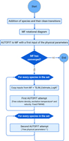 |
Fig. A.1 Flowchart of the MADCUBA macro that automates the line identification process. The asterisk (*) indicates that physical parameters are kept free whenever possible, following the criteria described in the text. |
This estimate is derived from the velocity-integrated intensity obtained by integrating the line emission in the velocity range defined by the linewidth.
Once appropriate inputs are obtained for all the species, a first AUTOFIT is performed in two rounds. In the first round, the FWHM remains fixed, and each species is fitted individually without taking into account the contribution from other species (disabling the ALL SPECIES flag in AUTOFIT). During this first step, brighter and unblended molecules converge easily and independently. The converged molecules provide constraints that will help in the second AUTOFIT iteration, which will try to fit all the species, including those blended. In this second round, the FWHM is left free and the contribution of all blended species is properly taken into account (enabling the ALL SPECIES flag in AUTOFIT).
We have tried to leave as many free physical parameters as possible in order to have the most unforced solution. However, for species with limited transitions, poor energy coverage, or blended lines, we adopted a hierarchical approach by fixing parameters when AUTOFIT does not converge: i) first FWHM, because usually this parameter can easily be obtained from the observed spectra; ii) V is fixed next, using the systemic velocity (V0) as a reference to constrain velocity shifts, since large deviations from this value are not expected; and iii) Tex is fixed when only one transition is available, as for example for or C18O, or when the number of transitions with different enough energies is not sufficient to make the fit to converge. In our approach, we never fixed N. Although this procedure is largely automated, the resulting fit must be visually inspected to ensure consistency with the observations, and this last step should be done manually. For a flowchart of the process, see Fig. A.1. Note that if MF does not converge, the automated macro stops. This could be due to MF not being present in the spectra, being too weak to be properly fit, or due to incorrect initial guesses. In the latter case, we should investigate the reason and, if possible, adjust the initial guesses.
Appendix B Generation of the maps (N)
To generate the Tex and N maps we used the SLIM module to fit the spectra on a pixel-by-pixel basis. MADCUBA provides a built-in tool to generate the integrated intensity map (moment 0), velocity field (moment 1), and velocity dispersion (moment 2) maps for selected transitions. To derive the moment maps, we selected an unblended transition for each of the three molecules of interest. For GA the transition 3510,26 → 359,27 at 220.055 GHz, for EG the transition 241,24 → 231,23 at 217.45 GHz, and for MF the transition 173,14 → 163,13 at 218.298 GHz.
To generate the Tex and N maps, we are using the spectral cube (spw0 and spw1) within a user-defined region of interest. The procedure performs the analysis only on pixels with a S/N above a given threshold in the moment 0 map, which in our case was S/N > 3. A preliminary rotational diagram analysis, for each pixel, is used to estimate the initial guesses for Tex and log N, as detailed in Sect. A. The velocity (V) and linewidth (FWHM) parameters are extracted from the line velocity (moment 1) and velocity dispersion (moment 2) maps, respectively. Moment maps were generated with a built-in tool from MADCUBA. The AUTOFIT routine inside SLIM is then executed for each pixel to perform a full LTE fit. The MADCUBA procedure generates as output a SLIM product containing the individual pixel-by-pixel fits, and the log(N), Tex, V, and FWHM maps. The only difference with the macro defined in Sect. A is that this procedure only takes into account the molecule that we are fitting, and not the contribution of all the other molecules. The provided maps have two channels: channel 1 contains the fitted values, while channel 2 stores the associated uncertainties.
Appendix B.1 Uncertainty N and Tex maps
We present the relative uncertainty maps of the column density (N; Fig. B.1) and excitation temperature (Tex; Fig. B.2) maps derived from the spectral fitting, in order to assess the reliability of the obtained physical parameters.
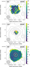 |
Fig. B.1 Relative error from the column density (N) maps derived for EG (top), GA (middle), and MF (bottom), respectively. Black contours correspond to the continuum emission at 5σ, 10σ, 20σ, 30σ, 60σ, 90σ, 180σ, 220σ, and 260σ with σ = 0.28 mJy beam−1. The red cross indicates the continuum peak position. The red ellipses outlined in white show the location and size of the dust continuum core AG318−c9 as estimated by Coletta et al. (2025). The hatched ellipse shown on the bottom left corner represents the synthesised beam of the interferometer. |
Appendix B.2 Molecular transitions used for N and Tex maps for ethylene glycol and glycolaldehyde
We present the molecular transitions used in the MADCUBA pixel-by-pixel fits for EG and GA.
Appendix C Zoomed-in line identification spectra
Figures C.1 and C.2 presents zoomed-in versions of the spw0 and spw1 spectra, respectively, shown in Sect. 5.1, aimed at better illustrating the weaker molecular lines used for line identification.
Appendix D Complete version of physical parameters table
Table D.1 presents the complete set of physical parameters derived from the SLIM analysis towards AG318−c9. Only a portion of this table is shown in the main text (Table 3).
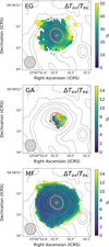 |
Fig. B.2 Relative error from excitation temperature (Tex) maps derived for EG (top), GA (middle), and MF (bottom), respectively. Black contours correspond to the continuum emission at 5σ, 10σ, 20σ, 30σ, 60σ, 90σ, 180σ, 220σ and 260σ with σ = 0.28 mJy beam−1. The red cross indicates the continuum peak position. The red ellipses outlined in white show the location and size of the dust continuum core AG318−c9 as estimated by Coletta et al. (2025). The hatched ellipse shown on the bottom left corner represents the synthesised beam of the interferometer. |
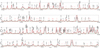 |
Fig. C.1 Same as Fig. 2 but with a zoomed-in y-axis to better highlight the weaker transitions and the quality of the spectral fit. |
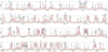 |
Fig. C.2 Same as Fig. 3 but with a zoomed-in y-axis to better highlight the weaker transitions and the quality of the spectral fit. |
Results of the SLIM fits of the species analysed towards AG318−c9, sorted by increasing number of atoms.
All Tables
Results of the SLIM fits of the species analysed towards AG318−c9. Only a portion of the table is shown here. The complete table is available in Appendix D.1.
Results of the SLIM fits of the species analysed towards AG318−c9, sorted by increasing number of atoms.
All Figures
|
Fig. 1 ALMA map of the continuum emission at 1.38 mm of the AG318.9477−0.1960 clump (left) and a zoom-in on core 9 (right). The white contours correspond to 5σ, 10σ, 20σ, 30σ, 60σ, 90σ, 180σ, 220σ, and 260σ, with σ ∼ 0.28 mJy beam−1. The cyan ellipses surrounded by black show the position and size of each core. In particular, the size of core 9 is 0.″66 × 0.″57, with a position angle of PA=42°. The synthesised beam (0.″46 × 0.″37, PA=7°) is shown in the bottom left corner. |
| In the text | |
|
Fig. 2 Spectra of spw0 towards core 9 of the AG318.9477−00.1960 clump. The black histogram and its grey shadow are the observational spectrum, and the red curve indicates the LTE fit after taking into account the contribution of all the species (see Table 3 and its complete version in Appendix D.1). The horizontal dashed green line indicates the 5σ ≈ 1.35 K level, with σ being the noise (σ ∼ 0.28 K). Only transitions contributing at ≥ 5σ are labelled. The vertical dashed black lines indicate the position where ν was converged. U labels indicate unidentified transitions. |
| In the text | |
|
Fig. 3 Spectra of spw1 towards core 9 of the AG318.9477−00.1960 clump. The black histogram and its grey shadow are the observational spectrum, and the red curve indicates the LTE fit after taking into account the contribution of all the species (see Table 3 and its complete version in Appendix D.1). The horizontal dashed green line indicates the 5σ ≈ 1.35 K level, with σ being the noise (σ ∼ 0.28 K). Only transitions contributing at ≥5σ are labelled. The vertical dashed black lines indicate the position where ν was converged. U labels indicate unidentified transitions. |
| In the text | |
|
Fig. 4 Column density comparison for all common species between AG318−c9 (x-axis) and G31 (y-axis). The solid black line indicates the 1:1 relation. The dark and light orange shaded regions represent deviations within 0.5 dex and 1.0 dex from equality, respectively. |
| In the text | |
|
Fig. 5 Top: comparison of molecular abundances (X = N/H2) towards G31 (blue bars) and AG318−c9 (orange bars), sorted by molecular groups and by the abundance of AG318−c9 inside each group. The species are grouped on the x-axis according to their detection status. Left: detected in both sources. Middle: detected in G31 alone. The orange triangles represent the corresponding upper limits for AG318−c9. Right: reported in AG318−c9. Bottom: logarithm of the ratio of the abundances of the two sources. HC3N* represents the group composed of HC3N, HC3N (v6 = 1), HC3N (v7 = 1), and HC3N (v7 = 2). |
| In the text | |
|
Fig. 6 Selection of GA transitions observed and fit (see Sect. 6.1). The black histogram and its grey shadow are the observational spectrum, and the red curve is the cumulative LTE fit considering all detected species. The blue curve is the fit of the individual transitions. The horizontal dashed green line indicates the 5σ level, corresponding to ∼1.35 K. Only transitions contributing at ≥5σ are labelled. The plots are sorted by decreasing intensity of the GA transitions (blue line). The upper left corner of each panel indicates the EUP of the corresponding GA transition. When multiple GA transitions are shown in the same panel, the EUP values are listed from top to bottom following the left-to-right order of the transitions. |
| In the text | |
|
Fig. 9 Integrated-intensity maps for EG (left), GA (middle), and MF (right). The white contours correspond to the continuum emission at 5σ, 10σ, 20σ, 30σ, 60σ, 90σ, 180σ, 220σ, and 260σ with σ = 0.28 mJy beam−1, and the red cross shows its peak position. The red ellipses surrounded by white show the location and size of the dust continuum core AG318−c9 as estimated by Coletta et al. (2025). The hatched ellipse shown in the bottom left corner represents the synthesised beam of the interferometer. |
| In the text | |
|
Fig. 10 Column density (N) maps (top row) and excitation temperature (Tex) maps (bottom row) derived for EG (left), GA (middle), and MF (right). The corresponding relative errors are shown in Appendix B.1. The black contours correspond to the continuum emission at 5σ, 10σ, 20σ, 30σ, 60σ, 90σ, 180σ, 220σ, and 260σ with σ = 0.28 mJy beam−1, and the red cross shows its peak position. The red ellipses surrounded by white show the location and size of the dust continuum core AG318−c9 as estimated by Coletta et al. (2025). The hatched ellipse shown in the bottom left corner represents the synthesised beam of the interferometer. |
| In the text | |
|
Fig. 11 Radial profiles derived from the column density (N; top) and excitation temperature (Tex; bottom) maps. The blue, red, and green curves correspond to EG, GA, and MF, respectively. The shaded areas indicate the measurement uncertainties (see Appendix B.1). The bar in the lower left corner indicates the radius corresponding to the geometric mean of the synthetic beam. |
| In the text | |
|
Fig. A.1 Flowchart of the MADCUBA macro that automates the line identification process. The asterisk (*) indicates that physical parameters are kept free whenever possible, following the criteria described in the text. |
| In the text | |
|
Fig. B.1 Relative error from the column density (N) maps derived for EG (top), GA (middle), and MF (bottom), respectively. Black contours correspond to the continuum emission at 5σ, 10σ, 20σ, 30σ, 60σ, 90σ, 180σ, 220σ, and 260σ with σ = 0.28 mJy beam−1. The red cross indicates the continuum peak position. The red ellipses outlined in white show the location and size of the dust continuum core AG318−c9 as estimated by Coletta et al. (2025). The hatched ellipse shown on the bottom left corner represents the synthesised beam of the interferometer. |
| In the text | |
|
Fig. B.2 Relative error from excitation temperature (Tex) maps derived for EG (top), GA (middle), and MF (bottom), respectively. Black contours correspond to the continuum emission at 5σ, 10σ, 20σ, 30σ, 60σ, 90σ, 180σ, 220σ and 260σ with σ = 0.28 mJy beam−1. The red cross indicates the continuum peak position. The red ellipses outlined in white show the location and size of the dust continuum core AG318−c9 as estimated by Coletta et al. (2025). The hatched ellipse shown on the bottom left corner represents the synthesised beam of the interferometer. |
| In the text | |
|
Fig. C.1 Same as Fig. 2 but with a zoomed-in y-axis to better highlight the weaker transitions and the quality of the spectral fit. |
| In the text | |
|
Fig. C.2 Same as Fig. 3 but with a zoomed-in y-axis to better highlight the weaker transitions and the quality of the spectral fit. |
| In the text | |
Current usage metrics show cumulative count of Article Views (full-text article views including HTML views, PDF and ePub downloads, according to the available data) and Abstracts Views on Vision4Press platform.
Data correspond to usage on the plateform after 2015. The current usage metrics is available 48-96 hours after online publication and is updated daily on week days.
Initial download of the metrics may take a while.