


| Issue |
A&A
Volume 711, July 2026
|
|
|---|---|---|
| Article Number | A237 | |
| Number of page(s) | 26 | |
| Section | Planets, planetary systems, and small bodies | |
| DOI | https://doi.org/10.1051/0004-6361/202558747 | |
| Published online | 17 July 2026 | |
ATREIDES
II. Detection of a polar orbit for HAT-P-26 b, a fluffy planet in the Neptunian ridge
1
School of Physics and Astronomy, China West Normal University,
Nanchong
637009,
PR China
2
Max-Planck-Institut für Astronomie,
Königstuhl 17,
69117
Heidelberg,
Germany
3
Observatoire Astronomique de l’Université de Genève,
Chemin Pegasi 51b,
1290
Versoix,
Switzerland
4
Department of Physics, University of Warwick,
Gibbet Hill Road,
Coventry
CV4 7AL,
UK
5
Centre for Exoplanets and Habitability, University of Warwick,
Gibbet Hill Road,
Coventry
CV4 7AL,
UK
6
Centro de Astrobiología,
CSIC-INTA, Camino Bajo del Castillo s/n,
28692
Villanueva de la Cañada,
Madrid,
Spain
7
Université Côte d’Azur, Observatoire de la Côte d’Azur, CNRS, Laboratoire Lagrange,
France
8
CFisUC, Departamento de Física, Universidade de Coimbra,
3004-516
Coimbra,
Portugal
9
LTE, Observatoire de Paris, Université PSL, Sorbonne Université, CNRS,
75014
Paris,
France
10
Instituto de Astrofísica e Ciências do Espaço, Universidade do Porto,
CAUP, Rua das Estrelas,
4150-762
Porto,
Portugal
11
Departamento de Fısica e Astronomia, Faculdade de Ciências, Universidade do Porto,
Rua do Campo Alegre,
4169-007
Porto,
Portugal
12
Yunnan Observatories, Chinese Academy of Sciences,
Kunming,
China
13
Key Laboratory for the Structure and Evolution of Celestial Objects, Chinese Academy of Sciences,
Kunming,
China
14
International Centre of Supernovae, Yunnan Key Laboratory,
Kunming,
China
15
European Southern Observatory,
Alonso de Córdova 3107,
Vitacura,
Región Metropolitana,
Chile
16
Tennessee State University (retired),
Nashville,
TN
37209
USA
17
School of Physics and Astronomy, University of Leicester,
Leicester
LE1 7RH,
UK
18
Rugby School,
Lawrence Sheriff St,
Rugby,
Warwickshire,
CV22 5EH,
UK
19
INAF – Osservatorio Astrofisico di Torino,
Via Osservatorio 20,
10025
Pino Torinese,
Italy
20
Centre for Space Domain Awareness, University of Warwick,
Coventry
CV4 7AL,
UK
21
Instituto de Astrofísica de Canarias (IAC),
38205
La Laguna,
Tenerife,
Spain
22
Departamento de Astrofísica, Universidad de La Laguna (ULL),
38206
La Laguna,
Tenerife,
Spain
23
Instituto de Astrofísica de Canarias,
38205
La Laguna,
Tenerife,
Spain
24
Universidad de La Laguna, Dept. Astrofísica,
38206
La Laguna,
Tenerife,
Spain
25
Astronomy Unit, Queen Mary University of London,
Mile End Road,
London
E1 4NS,
UK
26
Department of Physics and Astronomy, University of Delaware,
217 Sharp Lab,
Newark,
DE
19716,
USA
27
Département de Physique, Institut Trottier de Recherche sur les Exoplanètes, Université de Montréal, Montréal,
Québec
H3T 1J4,
Canada
28
Department of Earth, Atmospheric and Planetary Sciences, Massachusetts Institute of Technology,
77 Massachusetts Avenue,
Cambridge,
MA
02139,
USA
★ Corresponding author: This email address is being protected from spambots. You need JavaScript enabled to view it.
Received:
22
December
2025
Accepted:
5
May
2026
Abstract
Context. HAT-P-26 b is a well-characterized Neptunian exoplanet (Rp ≃ 6.33 R⊕) orbiting a K1V star. It lies within the Neptunian ridge (Porb ≃ 4.2345 days), following a moderately eccentric orbit (e ≃ 0.12) and hosting a water-rich atmosphere. The possible presence of a stellar companion hinted at by near-infrared (NIR) spectral emission, along with candidate planetary companions inferred from transit timing variations, calls for further investigations of the system architecture. Hence, the HAT-P-26 system is a prominent target for investigating the atmospheric and dynamical evolution of exo-Neptunes and, in particular, via the study carried out by the Ancestry, Traits, and Relations of Exoplanets Inhabiting the Desert Edges and Savanna (ATREIDES) collaboration.
Aims. We combined three transit observations of HAT-P-26 b using ESPRESSO on ESO’s VLT to precisely characterize its orbital architecture and to investigate whether it has a misaligned orbit, as reported in cases of other evaporating and eccentric planets in the ridge.
Methods. We employed the ANTARESS workflow to perform a careful and robust data reduction. We explored the system’s orbital architecture using the in-built Rossiter-McLaughlin Revolutions (RMR) technique.
Results. HAT-P-26 b exhibits a polar orbit (projected obliquity angle of λ = −78−13+13∘ and a 3D true obliquity angle of ψ = 85−5+5∘). This places it alongside GJ 436 b, HAT-P-11 b, and GJ 3470 b as polar-orbit and eccentric planets lying within the ridge population. It has the lowest density (0.40 ± 0.10 g cm−3) of these four planets, placing it near the density brink where full atmospheric erosion after early disk-driven migration or tidal disruption after high-eccentricity migration has been proposed to occur. Our dynamical analysis suggests that the observed polar orbit might either be a transient state arising from orbital-plane precession or a relic of high-eccentricity migration via Von Zeipel–Lidov–Kozai cycles driven by an inclined stellar companion. We note that in the latter case, the existence of planet c would be strongly disfavored.
Conclusions. HAT-P-26 b stands out as a special target in the Neptunian ridge, owing to its low density and polar orbit. The current dynamical analysis is limited by the uncertainties surrounding companion(s) in this system. As better constraints on the companion(s) become available, it will be particularly interesting to further explore the origin of this fluffy ridge Neptune through a joint analysis of migration, evaporation, tidal disruption, and inflation. Our results also demonstrate the importance of homogeneous data reduction when combining multi-epoch transit observations for accurate spin–orbit characterization.
Key words: techniques: photometric / techniques: radial velocities / planets and satellites: dynamical evolution and stability / planets and satellites: fundamental parameters / planet-star interactions / planets and satellites: individual: HAT-P-26
UKRI Future Leaders Fellow.
SNSF Postdoctoral Fellow.
© The Authors 2026
 Open Access article, published by EDP Sciences, under the terms of the Creative Commons Attribution License (https://creativecommons.org/licenses/by/4.0), which permits unrestricted use, distribution, and reproduction in any medium, provided the original work is properly cited.
This article is published in open access under the Subscribe to Open model.
Open Access funding provided by Max Planck Society.
1 Introduction
The short-period Neptunian desert refers to the significant scarcity of Neptunian planets with short orbital periods where observational biases have been ruled out (e.g., Mazeh et al. 2005; Lecavelier Des Etangs 2007; Davis & Wheatley 2009; Szabó & Kiss 2011; Lundkvist et al. 2016; Mazeh et al. 2016; Castro-González et al. 2024a). In the super-Neptune regime, beyond the Neptunian desert (Porb ≲ 3.2 days; Castro-González et al. 2024a), planet occurrences based on Kepler data revealed an over-density of planets in the orbital period range 3.2 days ≲ Porb ≲ 5.7 days referred to as the Neptunian ridge (Castro-González et al. 2024a), which separates the desert from the mildly populated Neptunian savanna at larger orbital distances (Bourrier et al. 2023), as shown in Fig. 1. Currently, three main mechanisms – disk-driven migration (DDM; e.g., Goldreich & Tremaine 1979; Lin et al. 1996; Frazier et al. 2023), high-eccentricity tidal migration (HEM; e.g., the Von Zeipel– Lidov–Kozai (ZLK) cycles; von Zeipel 1910; Kozai 1962; Lidov 1962), and photoevaporation (e.g., Owen & Jackson 2012; Owen & Wu 2013), have been proposed to be responsible for the distribution of close-in exo-Neptunes.
The spin–orbit angle, which refers to the angle between a planet’s orbital axis and its host star’s spin axis, is a key tracer of dynamical history (e.g., Dawson & Johnson 2018; Albrecht et al. 2022). While primordial spin–orbit alignment inherited from an aligned planetary disk is expected and has been observed in some young planets and compact multiplanet systems (e.g., Feinstein et al. 2021; Frazier et al. 2023; Radzom et al. 2024), moderate misalignments have also been reported (e.g., Bate 2018; Hjorth et al. 2021; Bourrier et al. 2022; Biddle et al. 2025; Yu et al. 2025). Such primordial misalignments may arise from magnetic interactions, chaotic accretion, or disk tilting by companions (Lai et al. 2011; Bate et al. 2010; Batygin 2012). After disk dispersal, violent dynamical processes, including planet–planet scattering, secular interactions, or ZLK cycles (e.g., Chatterjee et al. 2008; Naoz et al. 2011; von Zeipel 1910; Kozai 1962; Lidov 1962), can induce high misalignments. A large spin–orbit angle is generally interpreted as tentative evidence for such gravitational interactions after the disk dissipated.
Some warm Neptunes in the ridge are preferentially located in near-polar orbits (Bourrier et al. 2018, 2023; Albrecht et al. 2021, 2022; Castro-González et al. 2024a; Espinoza-Retamal et al. 2024; Knudstrup et al. 2024; Handley et al. 2025; Yee et al. 2025). In addition, these planets often show nonzero orbital eccentricities (Correia et al. 2020) and, for three of them, there are clear signs of atmospheric evaporation (GJ 436 b, GJ 3470 b, HAT-P-11 b; Ehrenreich et al. 2015; Bourrier et al. 2018; Allart et al. 2018), suggesting that they may share a common evolutionary history, possibly linked to HEM (Bourrier et al. 2025; Castro-González et al. 2026). Although the specific timing and mechanism behind the establishment of the polar architecture remain unclear, once established, it is thought to remain stable over Gyr timescales due to its insensitivity to inclination damping during tidal dissipation (Lai 2012; Louden & Millholland 2024).
Sethi & Millholland (2025) compared 12 misaligned and 12 aligned Neptune-sized planets with MESA models, finding that the misaligned sample is preferentially inflated and requires tidal heating to reproduce the observed radius results. In addition to the tidal dissipation (Jackson et al. 2008; Leconte et al. 2010), other mechanisms, such as Ohmic dissipation (Batygin & Stevenson 2010; Thorngren & Fortney 2018; Batygin 2025), can also contribute to inflating the planets. The resulting radius inflation, in turn, enhances the star–planet tidal interaction, thereby accelerating orbital circularization and/or spin synchronization (Bodenheimer et al. 2001; Lu et al. 2025; Sethi & Millholland 2025). Meanwhile, such tidal heating can also significantly affect the dynamical (e.g., atmospheric evaporation) and chemical (e.g., CH4 depletion) properties of the planetary atmosphere (Sing et al. 2024; Welbanks et al. 2024).
The distribution of the Neptune population has been found to be density-dependent: the desert is dominated by high-density planets (ρp > 1 g cm−3), the ridge contains a mixture of densities, and the savanna is dominated by low-density planets (ρp < 1 g cm−3; Castro-Gonzàlez et al. 2024b; Bourrier et al. 2025). In the ridge, the density distribution appears to be bimodal, with a lower mode at ~0.4-0.7 g cm−3 and a higher mode at ~1.7 g cm−3 (Castro-Gonzàlez et al. 2026). Low-density planets are expected to lose a greater fraction of their primordial mass compared to high-density planets (e.g., Lecavelier Des Etangs 2007) and the three Neptunes observed to be evaporating are within the ridge. Based on these observations, together with a detailed analysis of the mass and radius distribution, Bourrier et al. (2025) proposed a unified picture that combines migration and photoevaporation to explain the distribution of Neptunes. They suggested that a density brink within the ridge marks the location where atmospheric erosion fully erodes low-density Neptunes. At shorter periods into the desert, only high-density Neptunes or low-density Neptunes migrating after the saturated XUV phase of their host star (Owen & Lai 2018) can survive. The density brink has also been interpreted as the outcome of tidal disruption of HEM-migrated Neptunes, since higher-density planets can survive at smaller periastron distances, whereas lower-density ones are more easily disrupted (Castro-González et al. 2026).
Overall, the Neptunian ridge, corresponding to an orbital region with a relatively high planet occurrence, is suspected to be a hotspot for planet migration driven by both DDM and HEM (Castro-González et al. 2024a; Bourrier et al. 2025). This work aims to constrain the dynamical history of the ridge planet HAT-P-26 b by investigating its orbital architecture. HAT-P-26 b ( , Mp = 18.75 ± 2.23 M⊙, ρp = 0.4 ± 0.1 g cm−3,
  , age=
 Gyr, Hartman et al. 2011), orbiting an K1V star, has been reported to be undergoing atmospheric evaporation, as indicated by the detection of excess He I absorption in low-resolution transit observations (Vissapragada et al. 2022). This interpretation, however, has been challenged by recent high-resolution He I triplet observations (Orell-Miquel et al. 2026). A measurement of HAT-P-26 b projected spin–orbit angle (λ = 18° ± 49°) was derived by Mancini et al. (2022) using HARPS-N spectra, although the large uncertainty (due to the lack of coverage for the start of the transit and the low data quality at its endpoints) prevents a definitive conclusion about the alignment of the system.
This work is part of the ATREIDES collaboration (Bourrier et al. 2025), which is aimed at understanding the formation and evolution of close-in Neptunian exoplanets at the population level by investigating the atmospheric and orbital dynamical properties of approximately 60 close-in Neptunes using spectroscopic and photometric observations. This paper is structured as follows: In Sect. 2, we describe the photometric and spectroscopic observations and the corresponding data reduction. In Sect. 3, we present the transit light curve fitting and in Sect. 4, we refine the stellar parameters. In Sect. 5, we investigate the system’s orbital architecture using the RMR method. In Sect. 6, we discuss the dynamics for the system and in Sect. 7, we provide a summary of our work.
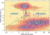 |
Fig. 1 Distribution of orbital period versus radius for close-in exoplanets. The boundaries for the refined classification (Neptunian desert, ridge, and savanna; Castro-González et al. 2024a) are shown as dashed lines. Neptunes with well-measured 3D spin–orbit angles (precision better than 30° in the TEPCat catalog1) are marked with crosses. Squares represent planets with (red edge) or without (magenta edge) escaping H/He detections. HAT-P-26 b is marked with a star. The radius and mass values are taken from the NASA Exoplanet Archive2. |
2 Observations and data reduction
2.1 Transit photometry
2.1.1 Observation
We obtained a photometric transit with NGTS (Next Generation Transit Survey; Wheatley et al. 2018) on 2022 July 03, simultaneous to one of the ESPRESSO spectroscopic observations, with an aim to accurately measure the transit time. In brief, NGTS is a photometric facility consisting of twelve 20 cm diameter telescopes situated at ESO’s Paranal Observatory in Chile. Each NGTS camera is independently and robotically controlled, observes using a custom red-optical filter (520–890 nm), and has a wide field of view (FoV) of 2.6 × 2.6 degrees. By observing the same star using multiple NGTS telescopes simultaneously, we can achieve high-precision photometric observations of individual exoplanet transit events (Smith et al. 2020; Bryant et al. 2020).
2.1.2 Data reduction
We observed HAT-P-26 with seven NGTS cameras using an exposure time of 10 seconds for all cameras. A custom aperture photometry pipeline was used to reduce the NGTS observations. The aperture radii ranged from 3.5 to 4 pixels for the different cameras. A set of unblended comparison stars similar to HAT-P26 in apparent magnitude, stellar color, and CCD position were selected using Gaia (Gaia Collaboration 2018, 2023) and used to produce differential flux time series.
2.2 Long-term photometric monitoring
We collected long-term, nightly photometric observations of HAT-P-26 for the purpose of monitoring starspot activity with the Tennessee State University Celestron 14-inch (C14) automated imaging telescope (AIT) located at Fairborn Observatory in southern Arizona of the United States (e.g., Eaton et al. 2003). The AIT employs an STL-1001E CCD camera with a pixel scale of 1.2 arcsec pixel−1 and a FoV of 21 × 21 arcmin. We have acquired 871 observations (excluding occasional transit observations) during the 12 observing seasons from 2012–2013 to 2023–2024. The observations were made through a Cousins R filter with an SBIG STL-1001E CCD camera. Each nightly observation consists of between five and ten consecutive exposures of the HAT-P-26 FoV. The individual frames are co-added and reduced to differential magnitudes in the sense HAT-P-26 minus the mean brightness of four constant comparison stars in the same field. Further details of our observing and data reduction procedures can be found in Sing et al. (2015).
2.3 Spectroscopic observations
2.3.1 Observation
We collected four ESPRESSO spectroscopic transit observations of HAT-P-26 b on 2021 March 24 (PID: 106.21M2.004, PI: Pepe, F.), 2021 April 10 (PID: 1104.C-0350(J), PI: Pepe, F.), 2022 July 03 (PID: 109.23FU.005, PI: Lafarga, M.), and 2024 May 02 (PID: 112.25BG.006, PI: Bourrier, V.). The first two visits were obtained as part of the Guaranteed Time Observations (GTO). ESPRESSO (Pepe et al. 2021) is an ultra-stable, fibre-fed spectrograph covering the wavelength range 378–789 nm, mounted on the Very Large Telescope (VLT) at ESO’s Paranal Observatory in Chile. These observations utilized the 1-UT configuration, with UT1 used for the first three visits and UT3 for visit on 2024 May 02, operating in HR21 mode (with a binning of 2 × 1). This configuration provides a resolving power of R = 138 000 and a pixel size of 500 m/s. In addition to monitoring the target with fibre A, simultaneous sky monitoring was performed with fibre B to remove sky emission. A standard spectral extraction workflow, including bias and dark subtraction, flat-field correction, bad pixel correction, 2D spectral extraction, blaze correction, and wavelength calibration, was applied using the ESPRESSO Data Reduction Software (DRS) version 3.2.03. In our analysis, we used 2D echelle spectra (S2D) corrected for the blaze function and for barycentric radial velocity (BERV). The system parameters used in this study are presented in Table 1.
As shown in Fig. 2, all four observations covered the full transit duration of 2.46 hours and additionally included 1.7– 3.3 hours of out-of-transit observations as the baseline. These baseline observations are essential for accurately measuring the Rossiter-McLaughlin effect (hereafter, the RM effect). The majority of the observations were conducted at an airmass below 2.0, with the exception of the post-transit phase in the 2022 observations. Despite this, the relatively long exposure time of 700 seconds allowed us to achieve a sufficient signal-to-noise ratio (S/N) in the spectra, except for the last spectrum, which had a shorter exposure time of 200 seconds due to significant elongation of the target at very low altitude. The spectral quality from 2021 April 10 was noticeably poorer, with more than half of the spectra exhibiting an S/N ≤ 20. Given the identical exposure settings and similar weather conditions compared to March 24, 2021, we ruled out weather as the primary factor. We note that the atmospheric dispersion corrector (ADC) values in the headers are missing, indicating that the ADC was not operating properly that night. Consequently, we excluded from our subsequent analysis all data observed on the night of 2021 April 10, and the last data point on 2022 July 03.
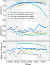 |
Fig. 2 Observational logs of the four ESPRESSO visits, including airmass, seeing, and S/N around 550 nm (orders 102 and 103). For each visit, the median exposure time and the mean value of the integrated water vapor (IWV) content are shown in the legend. Grey-shaded regions indicate the out-of-transit phases, highlighting the transit window. |
Properties of the HAT-P-26 system.
2.3.2 Data analysis
In this work, we employed Advanced and Neat Techniques for the Accurate Retrieval of Exoplanetary and Stellar Spectra (ANTARESS4, Bourrier et al. 2024) to clean the S2D data and derive the spin–orbit angle. ANTARESS is an end-to-end data analysis package, which aims to extract high-resolution exoplan-etary and stellar spectra accurately in a reproducible and robust way. This package has significant advantages in homogeneously handling multiple visits from one or several instruments, as it specifically accounts for relevant environmental and instrumental effects. More details are given in Bourrier et al. (2024).
To clean the S2D spectra, we followed the typical correction steps described in Sect. 4.2 of Bourrier et al. (2025), which include (1) noisy data exclusion; (2) blaze profile-based flux calibration; (3) telluric correction for H2O and O2, based on the Automatic Telluric Correction (ATC) method (Allart et al. 2022) using the HITRAN database (Rothman et al. 2013); (4) correction for Earth atmospheric diffusion; (5) cosmic ray correction; (6) ESPRESSO “wiggle” modeling and correction. In addition to the typical corrections described above, we also performed a stellar line detrending in step (7). This method is designed to obtain an unbiased cross-correlation function (CCF) time series by correcting for potential systematic trends between line properties and environmental or housekeeping parameters (e.g., S/N and time) in the out-of-transit spectra. After those corrections, the data quality has improved significantly compared to raw S2D data. Here, we highlight the improvements obtained by applying wiggle correction and stellar line detrending.
For the wiggle modeling, we use two sine components to represent the two strongest frequency peaks found in our transmission spectra. Similarly to previous studies (Bourrier et al. 2024, and references therein), the amplitude and frequency gradually varies with wavelength and time across all three of our visits. By characterizing how the phase and the chromatic coefficients of frequency and amplitude vary with the telescope pointing coordinates, we successfully reconstructed the observed variations of the wiggle feature using a physical model. After applying the wiggle correction, the root-mean-square (RMS) of the HAT-P-26 b transmission spectra was reduced by 9.39%, 9.83%, and 1.45% for the visits on 2021 March 24, 2022 July 03, and 2024 May 02, respectively (see Fig. A.1 for example). The relatively modest improvement for the 2024 May 02 dataset is due to its lower S/N, which means that most of the wiggle effects are smaller than the data noise and thus have a limited impact on our results.
For the stellar line detrending, the mean line profile (CCF profile), calculated by cross-correlating the S2D data with a custom CCF mask (see also Sect. 5.1), is used to extract the overall spectral line properties. Fits performed with a Gaussian profile best reproducing the HAT-P-26 CCF allowed us to measure the spectral line contrast (contrast), full width at half maximum (FWHM), and radial velocities (RVs). For the exposures obtained on 2021 March 24, we found a significant trend between contrast and the root-sum-square S/N (snrQ) in the out-of-transit spectra, which is well fitted by a second-order polynomial (see Fig. A.2). A “vertical stretching” correction (see Bourrier et al. 2024), based on this fitted model, was applied to all individual lines over the entire time series to remove the effect of snrQ on the contrast.
3 Transit analysis
We performed a transit analysis of the NGTS photometric data to refine the planet parameters and precisely constrain the transit ephemeris. We fit the transit using transit models generated with the batman5 package (Kreidberg 2015) and sampled the parameters using a Markov chain Monte Carlo (MCMC) sampling method implemented using the EMCEE6 package (Foreman-Mackey et al. 2013). The following planetary parameters were included as free parameters in the transit fitting: the transit epoch, T0, the planet-to-star radius ratio, RP/R⋆, the scaled semimajor axis, a/R⋆, and the orbital inclination, i. All these parameters are constrained using uniform priors to ensure physically realistic values (see Table C.1). We also include the orbital period, Porb, in the analysis, but the period is tightly constrained using a Gaussian prior based on the results from Kokori et al. (2023, see our Table C.1). For the limb darkening coefficients we use the parameterization from Kipping (2013) and include the q1 and q2 parameters as free parameters, both constrained with a uniform prior to be between 0 and 1 to ensure a physically admissible stellar intensity variation. Given the results of Hartman et al. (2011) we model the orbit of HAT-P-26 b as eccentric. The orbital eccentricity, e, and argument of periastron, ω, are constrained using truncated Gaussian priors based on the results from Hartman et al. (2011, see Table C.1).
In addition to the transit model, we employed detrending models for each of the seven individual NGTS light curves. Each light curve is detrended using a linear model against airmass simultaneously with the transit fit, with the seven pairs of detrending coefficients included in the analysis as free parameters. In total, we obtained a set of 23 free parameters.
One of our aims here is to study how our new mid-transit time from the NGTS transit fits within the current studies. Thus, we computed the expected mid-transit time using the linear ephemeris reported in A-thano et al. (2023) (reference midtransit time 2455304.65209 and period 4.234503 d; see their Eq. (4)) and compared that to the one obtained directly by fitting the NGTS data above. We found that the NGTS transit occurs ∼4.1 min before expected time from the linear ephemeris and is also significantly different from the predicted sinusoid variations from A-thano et al. (2023). We note that A-thano et al. (2023) also derived ephemeris and TTV from a fit to only 33 of the transits. Using this other set, we obtained similar results, with differences in the transit timing residual less than the 1σ uncertainty. We performed our spectroscopic analysis using both the ephemerides derived from A-thano et al. (2023) and from our fit to the NGTS data. Our final results produce a negligible difference between each method.
The main planetary parameter results obtained from the NGTS transit analysis are reported in Table C.1, with the results for the detrending coefficients reported in Table C.2. We show the NGTS data and the model in Fig. 3 and the posteriors for each parameter in Fig. C.1. We reiterate that our analysis was performed on the individual camera light curves, treated as independent data sets and fitted simultaneously in a joint analysis (see Fig. C.2). We also note that the trend-like structure before the transit (driven by the data from the bottom-left panel in Fig. C.2) and the elevated points prior to the transit (driven by outlying points in the top-right light curve in Fig. C.2) shown in Fig. 3 are driven by outlying points in single NGTS camera light curves. Therefore, neither of them are expected to have significantly biased the inferred planetary parameters.
The NGTS bandpass covers a similar wavelength range as ESPRESSO (see Sect. 2.3) and so, the limb darkening coefficients u1 and u2 derived from the NGTS light curve should be suitable for the modeling of our spectroscopic transits (see Sect. 5.1). However, the limb darkening parameters derived from the NGTS light curve exhibit broad posterior distributions, meaning that the NGTS photometry alone does not offer enough precision to tightly constrain the coefficients. Therefore, we chose to estimate the theoretical quadratic limbdarkening coefficients using the LDTk7 (Husser et al. 2013 Parviainen & Aigrain 2015) and ExoCTK8 (Bourque et al. 2021) tools, based on stellar parameters from Hartman et al. (2011). Specifically, within ExoCTK we adopted the Kurucz ATLAS9 (Kurucz 1993) and Phoenix ACES (Husser et al. 2013) stellar models. The resulting coefficients are as follows: u1 = 0.532 ± 0.003, u2 = 0.128 ± 0.004 for LDTk, u1 = 0.533 ± 0.003, u2 = 0.138 ± 0.004 for ExoCTK (Kurucz ATLAS9), and u 1 = 0.513 ± 0.003, and u2 = 0.110 ± 0.004 for ExoCTK (Phoenix ACES). We then adopted the weighted-mean values u1 = 0.526 and u2 = 0.1253 for the subsequent analysis. To account for potential systematic offsets between different stellar model predictions, we assigned relatively large uncertainties of 0.05 to both coefficients (see Table 1).
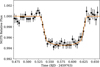 |
Fig. 3 NGTS transit data taken on 2022 July 03. Black data points show the average of all seven cameras used binned to 5 minutes and airmass-detrended, and orange line shows the best fit model. |
4 Stellar parameters
4.1 Fundamental stellar parameters
The stellar spectroscopic parameters (Teff, log g, vtur, and [Fe/H]) and chemical abundances were derived using the ARES+MOOG methodology as described in our previous works (e.g., Adibekyan et al. 2016; Delgado Mena et al. 2017; Sousa et al. 2021). We refer to the detailed description provided in Sect. 5.1 in Paper I (Bourrier et al. 2025). We could not derive the abundance of carbon due to the low Teff of this star, and we could not derive oxygen abundance due to the lack of reliable lines in the spectrum. However, we provide abundances of Mg, Si, Ni, Zn, and Y in Table 1 in the form of [X/H] ratios, i.e., the abundances with respect to the solar abundances obtained from a high resolution and high S/N spectrum of Vesta.
Despite the fact that this star has a metallicity typical of the thin disk, the abundances of the α elements are high ([α/Fe] = 0.09 dex). This star could belong to the high-α metalrich (hαmr) population (Adibekyan et al. 2011), which presents older ages than thin disk stars at the same metallicity, while remaining younger than the thick-disk population (Delgado Mena et al. 2019). To estimate the age of this star, we employed the abundance ratios of certain elements (also called chemical clocks) that provide stellar ages from empirical calibrations obtained with high quality isochronal ages from stars within the HARPS-GTO survey. In particular, we used the 3D formulas in table 10 of Delgado Mena et al. (2019) for the chemical clocks [Y/Mg], [Y/Zn] and [Y/Si], all yielding ages above 11 Gyr (refer to Table 1), and confirming that HAT-P-26 belongs to the hαmr population. Indeed, this star has also been analyzed by Biazzo et al. (2022), who found that it presents kinematic properties consistent with thin-thick disk transition. These authors also reported enhanced α elements abundance and an old age, supporting our results.
4.2 Stellar activity and rotation period
The stellar rotation period (Prot) of HAT-P-26 has not been previously established in the literature. Hartman et al. (2011) analyzed the HATNet photometry and reported no coherent periodic variability. They also used HIRES spectra (Vogt et al. 1994) to derive a chromospheric activity index of log R′HK = −4.992, consistent with HAT-P-26 being a chromospherically inactive star (i.e., log R′HK < -4.75; Vaughan & Preston 1980). The value of veq sin i⋆ reported by Hartman et al. 2011 (1.8 ± 0.5 km s−1), combined with the stellar radius derived in Sect. 4, places an upper limit for Prot of 25.6 ± 7.2 days. We note, however, that measuring reliable spectroscopic rotational velocities for slow rotators (veq sin i⋆ < 3 km s−1) is notoriously challenging, and therefore this estimate must be interpreted with caution. This, together with the known discrepancies between spectroscopic and RM-based determinations of veq sin i⋆ (e.g., Cegla et al. 2016; Triaud 2018; Bourrier et al. 2025), further motivates prudence in interpreting this upper limit. In the following, we first use our ESPRESSO-derived log R′HK value to estimate Prot through empirical activity-rotation relations, and then further investigate rotation-induced periodicities in our AIT photometry.
We derived the S-index from the ESPRESSO spectra with ACTIN29 (Gomes da Silva et al. 2018, 2021) and used pyrhk10 to derive the log R′HK calibrated onto the Mount Wilson scale (Vaughan et al. 1978). We obtained a value of log R'HK = −5.024 ± 0.045, computed as the median of the 113 individual measurements, with the uncertainty representing their standard deviation. We estimated the Prot of HAT-P-26 following the relations by Noyes et al. (1984) and Mamajek & Hillenbrand (2008), obtaining Prot = 45.6 ± 8.4 days and Prot = 48.7 ± 4.7 days, respectively. We also used the relations for K spectral types from Suárez Mascareño et al. (2016), obtaining Prot = 46.3 ± 3.7 days.
We first analyzed the AIT photometry using a Generalized Lomb-Scargle (GLS) periodogram (Zechmeister & Kürster 2009) to search for periodic sinusoidal-like modulations. For this purpose, we computed the GLS power spectrum over periods between 1.5 and 150 days, together with the corresponding window function (Fig. B.1). The periodogram shows several peaks at long periods, including a maximum around 120 days. However, none of them exceed the empirical 10% false alarm probability (FAP) level estimated through a block-bootstrap procedure. The structure of the window function displays prominent aliases in the same range, indicating that the peaks are likely related to the sampling rather than to coherent periodic signals.
We also modeled the AIT photometry using Gaussian process regression (Rasmussen & Williams 2006; Roberts et al. 2012) with a quasi-periodic kernel (Ambikasaran et al. 2015), a framework that has proven effective for capturing complex stellar activity signals exhibiting nonperiodic and nonsinusoidal behaviors in long time scales (Faria et al. 2016; Delisle et al. 2022; Castro-González et al. 2023, 2025). The parameter space was explored using the nested sampling implementation in dynesty (Speagle 2020), adopting 10 000 live points and a conservative stopping criterion of ∆Z < 10−5. We used wide uniform priors for the four kernel hyperparameters, namely, U(0,0.1) mag for the amplitude, U(0,200) days for the periodic length scale, U(0,20) for the periodic coherence scale, and U(1.5,150) days for the stellar rotation period.
In the left panel of Fig. B.2, we show the AIT photometric time series together with the median posterior activity model and its associated 1σ predictive interval. The right panel shows the posterior distribution of the stellar rotation period. Although the distribution exhibits a clear peak with a mode of ∼eq 35.4 days, the posterior does not fully converge into a single, well-defined solution. Instead, significant probability remains distributed across families of longer rotation periods that are still compatible with the AIT photometry. Consequently, we cannot robustly confirm a rotation period based on these data. This is further supported by the Bayesian evidence, which yields a logarithmic difference of +0.4 relative to the null hypothesis, indicating that the data do not provide enough support for a well-constrained periodic model.
Nevertheless, it is noteworthy that the 35-day peak is well aligned with the rotation interval predicted by the empirical activity-rotation relations. For this reason, we consider the 35-day signal as a plausible candidate for the true stellar rotation period, even if it cannot be formally established. In the context of our RMR analysis, therefore, we adopted an unconstrained rotation period for the final inference, reflecting the lack of compelling evidence for a specific value. However, as an informative test, we also explore the implications of assuming the 35-day period. Using a Gaussian fit to the posterior peak described above, we derive an approximate rotation period and associated uncertainty (Prot = 35.4 ± 6.1 days), which we used to assess how such a value would affect the inferred true obliquity.
5 RM effect revolutions
The RM effect is a spectroscopic distortion observed during a planetary transit, caused by the planet blocking part of the rotating stellar surface (Rossiter 1924; McLaughlin 1924). This effect provides a diagnostic for revealing the alignment between the planet’s orbital plane and the star’s rotational axis (3D spin–orbit angle). In this work, taking into account the slow stellar rotation and the small planet-to-star area ratio, we employed the RMR technique (Bourrier et al. 2021, 2022) to constrain the orbital architecture. We also compared our results with those obtained using the classical RM method, as described in Appendix E.
RMR is a well-established technique used to extract the planetary orbital architecture by fitting the intrinsic stellar CCF profiles (CCFs) from planet-occulted regions. Compared to the classical RM method, which relies on anomalous radial velocities derived from disk-integrated line profiles, the RMR technique jointly models all planet-occulted regions to better exploit the spectroscopic information. Therefore, it enhances the detection capability for weak RM signals and reduces biases introduced by variations in stellar line profiles along the transit chord. To carry out the RMR analysis, we begin by extracting the intrinsic CCF profiles for each observation (Sect. 5.1) and subsequently derive the mean spectral line properties from these profiles (Sect. 5.2). We then explored the most suitable surface model for the extracted RVs and analytical laws describing the evolution of the intrinsic CCF shapes along the transit chord (Sect. 5.3). Finally, we performed a global joint analysis of all parameters to infer the orbital architecture of the system (Sect. 5.4).
5.1 Intrinsic CCF profile calculations
To calculate the intrinsic CCF profiles, we first align the timeseries ANTARESS-cleaned S2D spectra to the stellar rest frame and scale the flux according to the theoretical transit model computed with the batman5 (Kreidberg 2015). A master out-of-transit spectrum was constructed by taking a weighted mean of the aligned and scaled spectra using an advanced method in ANTARESS. In short, the weights account not only for low-frequency variations (flux calibration, color effects, flux scaling) but also for high-frequency variations (tellurics, stellar lines) in pixel flux precision, thereby reducing systematic biases. Next, the S2D differential spectra are obtained by subtracting each aligned and scaled spectrum from the master spectrum. We use in-transit differential spectra to construct the intrinsic spectra, which represent the photospheric spectrum of the planet-occulted regions. Then, the CCFs were created by crosscorrelating each S2D intrinsic spectrum with a custom visitspecific CCF mask (see details in Bourrier et al. 2021 for the build process and in Cretignier et al. 2020 for the optimized line identification strategy). Finally, we obtained the intrinsic CCF profiles by normalizing the resulting CCFs to a common flux level, as shown in the top row of Fig. 5.
To evaluate the stability of the stellar CCF profiles derived from both the custom visit-specific CCF masks (generated from the master spectrum of individual visit) and the DRS K2 mask (built from the actual ESPRESSO spectral line list and depths of a K2-type star), we compared the standard deviations of the out-of-transit contrast and FWHM ( , normalized by their mean 〈x〉), and Keplerian RV residuals (RVres) time series derived from the CCF profiles generated with each mask. The results are listed in Table 2. A more direct comparison of the time series of Keplerian RVres can be found in Fig. A.3. Our results clearly demonstrate that using the custom CCF mask leads to a significant improvement in both stability and precision, as expected for a K-type star (Bourrier et al. 2023). In addition to the visitspecific mask, we also tested a common CCF mask generated from the combined master spectra of all three visits. In principle, the use of a common mask reduces visit-dependent biases in the CCF profiles. However, visit-specific masks perform significantly better than the common mask across all visits, yielding smaller uncertainties in the fitted λ, improved model fits (lower BIC values) and more consistent surface RVs (see Table 3 vs. D.1 and Table 4 vs. D.2). We attribute this improvement to possible variations in spectral line shapes between visits arising from slight changes in instrumental response, observing conditions, and/or stellar surface inhomogeneities. We therefore adopt the results derived from the visit-specific CCF masks as our final values, while noting that the two approaches yield mutually consistent results within the uncertainties.
5.2 Property extraction
To extract the properties for each intrinsic CCF profile, we modeled the profile with a Gaussian function, with parameters including the RV centroid, FWHM, and contrast. The posterior distributions of these parameters are sampled using the emcee6 MCMC algorithm (Foreman-Mackey et al. 2013), starting from uninformative priors. Specifically, an RV centroid prior of U(−2, +2) km s−1 (considering the projected stellar rotational velocity of ∼± 1.8km s−1; Hartman et al. 2011), a >FWHM prior of U(0,20) km s−1 (approximately three times the average width of local stellar lines), and a contrast prior of U(0,1). This emcee6 setting was explored using 100 walkers for 1500 steps with a burn-in of 500 steps. Our fitting results (Fig. D.1) show that the posterior probability distributions (PDFs) exhibit symmetric shapes and distinct peaks for all explored line properties in most of the observational data, except for exposures near the limb during each visit. The PDFs for these limb exposures are poorly constrained due to the lower intensity of the occulted regions and their partial coverage by the planet. Consequently, the first and last intrinsic profiles of each visit are excluded from the subsequent model analysis.
Comparison of properties of CCFs generated with the custom mask and the DRS K2 mask.
Results for the individual fits to intrinsic property time series.
Results for the joint fits to intrinsic profile time series.
5.3 Individual model exploration
To identify the optimal surface RV model (Cegla et al. 2016; Bourrier et al. 2017) and the analytical laws that describe the intrinsic line properties, we performed individual analyses for each property.
Since the surface RV model (Cegla et al. 2016) is influenced not only by the architecture of the planetary orbit, but also potentially by stellar surface motions, including differential rotation and convective shifts, we tested four different surface velocity models. First, we explored the baseline RV surface model (M1), which assumes solid-body rotation and adopts uniform priors of v sin i⋆ ~ U(0,5) km s−1 and λ ~ U(-π,π). We then tested whether the data was able to constrain convective blueshift effects in M2 and M3 by adding one or two convective blueshift components, respectively, c1, c2 ~ U(-3,3) km s−1, to the baseline model. Finally, we explored the possibility of surface differential rotation using M4 by introducing the stellar inclination term cos i⋆ ~ U(−1,1) and the shear parameter α ~ U(0,1). As shown in Table 3, the Bayesian information criterion (BIC) values for the different models are very similar and tend to favor the simplest model (M1). It is worth noting that because BIC imposes a strong penalty on model complexity, small BIC differences primarily indicate that the data lack sufficient statistical power to justify additional parameters, rather than demonstrating that the more complex models are physically disfavored. In this regime, the modest ∆BIC values are insufficient to support the inclusion of convective blueshift or differential rotation, suggesting that these effects are not well constrained by our current data.
Then, we explored the best analytical models describing how the FWHM and contrast of local CCF profiles vary with the projected center-to-limb distance on the stellar disk. Specifically, for both contrast and FWHM, we tested constant and linear models in three configurations: (1) applied individually to each visit, (2) fully common to all visits, and (3) a hybrid configuration with visit-specific constants but a common linear coefficient. Uniform priors were adopted for both the zero-order and first-order coefficients of the polynomial models: [–1, 1] and [–0.5, 0.5] for the contrast, and [0, 10] and [–2, 2] for the FWHM, respectively. We found that the data are best described by a common linear variation for contrast and a common constant for FWHM. This illustrates the stability of the stellar line profiles over at least a three-year period, within the precision of our data. The linear relation in contrast reflects a center-to-limb variation, which is clearly preferred by the data (e.g., Cavallini et al. 1985; Löhner-Böttcher et al. 2019; Bourrier et al. 2021). The data also hint at a similar trend of FWHM with projected distance, anti-correlated with the contrast (see Fig. 4). However, given the lower precision of FWHM measurements compared to the contrast, the BIC favors a constant model.
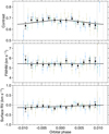 |
Fig. 4 Properties (dots) of the stellar surface occulted by the planet, along with the best-fit RMR model (M1, black lines) from the global fit. The measured properties from three visits are color-coded as in Fig. 2: blue for 2021 March 24, green for 2022 July 03, and yellow for 2024 May 02. The error bars represent the 1σ highest density intervals (HDIs), which correspond to the dashed green lines in Fig. D.1. To improve the visualization of the global fit, data points from all three visits are binned to a phase resolution of 0.0015 (black diamonds). The transit contacts are marked by the vertical dotted grey lines. |
5.4 Global RMR analysis
5.4.1 Projected spin–orbit angle
We then performed a global fit to the time-series intrinsic profiles in all visits to derive the orbital architecture. Following the discussion in Sect. 5.3, we adopted the baseline model (M1) settings to perform a global fit to the surface RV variations, with a common linear term for the contrast and a common constant value for the FWHM (hereafter model G1). The same uniform priors on v sin i⋆, λ, and the polynomial coefficients were applied in the global fit.
Figure D.2 displays the PDFs for the parameters in model G1 obtained from the global fit. The PDFs of all fitted parameters are well-converged, exhibiting prominent peaks and symmetric distributions. We found no significant correlations between the RV model parameters (λ and veq sin i⋆) and the fitted line profile parameters (FWHM, contrast, and continuum level), indicating that the RV model is derived independently and is largely insensitive to the fitted line shape parameters. We present the corresponding RMR model (solid dark line) for each property in Fig. 4. After subtracting the reconstructed intrinsic profiles (middle row in Fig. 5) from the data (top row in Fig. 5), no significant features remain in the residual map (bottom row in Fig. 5), indicating that our RMR model successfully captures the main features of the observational data.
5.4.2 3D spin–orbit angle
To explore the possibility of constraining the true (3D) spin– orbit angle, we extended our analysis to model G2, in which λ, cos i⋆, Prot, and R⋆ are sampled as free parameters. Specifically, the adopted priors are as follows: λ ~ U(-π, π), Prot ~ U(1,80) days, R* ~ N(0.91, 0.1) R⊙, and cos i* ~ U(−1,1). The projected rotational velocity (veq sin i⋆) and 3D spin–orbit angle (ψ) were then derived from the posterior distributions.
The PDFs of the fitting results are shown in Fig. D.3. A moderate stellar inclination, with two distinct peaks can be found for the PDF of cos i⋆. This double-peaked structure stems from the fact that RM signals do not allow for the northern and southern stellar hemispheres to be distinguished. Both configurations yield the same value of sin i⋆ and are therefore equally consistent with our observed veq sin i⋆. However, the values of ψ derived from i⋆ and its supplementary angle are not the same. According to Eq. (14) in Cegla et al. (2016), we have
 (1)
(1)
for the north case. Given i*,South = 180° – i*,North, we have
 (2)
(2)
for the south case. Therefore, the difference between the “north” and “south” cases arises from the sign change in the second term, i.e., the argument of the cos−1 function differs by 2 cos i⋆,North cos ip. Accordingly, the 3D spin–orbit angle is derived for the northern and southern configurations separately. We began by folding the MCMC samples over the northern configuration (cos i⋆ < 0), obtaining i⋆N and the corresponding ψN. The same procedure is then applied to the southern configuration (cos i⋆ > 0), yielding ψS.
5.4.3 Results
The fitting results for the global analyses of models G1 and G2 are presented in Table 4. We used the median of the PDFs as the best estimate of the model parameters. Since the posterior of i⋆ in model G2 is significantly asymmetric, we defined the 1σ uncertainty as the HDI enclosing 68.3% of the posterior probability to better capture the high-density region.
Both projected spin–orbit angles derived from models G1 ( ) and G2 (
 ) are consistent with the value reported by Mancini et al. (2022) (λ = 18° ± 49°) within 1σ, and with a higher level of precision. We obtained
  for the north-folded posteriors and
  for the south-folded posteriors. As the orbital inclination (ip) is close to 90°, the difference in ψ created by the second term in Eq. (2) is very small between the northern and southern configurations, and the PDFs for ψN and ψS are very similar. Therefore, we adopted an average value (ψcombined) of
  as the final 3D spin-orbit angle for HAT-P-26 b.
Because our photometry cannot significantly constrain Prot (see the discussion in Sect. 4.2), we adopted a physically motivated upper limit on Prot based on stellar population studies. For K-type main sequence stars, photometric surveys consistently show that rotation periods rarely exceed a few tens of days (e.g., McQuillan et al. 2014), providing an independent constraint far more stringent than what can be derived from the photometry of HAT-P-26 itself. Even adopting a conservative uniform prior of Prot ~ U(1,80) days, the RMR fit yields  km s−1, which combined with the implied Veq ≳ 0.58 km s−1 (using R* = 0.91 R⊙ and the longest allowed Prot), forces sin i⋆ to be small. We also tested a tighter prior of U(1,40) days, which yields nearly identical results (
 , see Fig. D.4). The resulting stellar inclination and true obliquity are therefore robust against the specific choice of the allowed prior upper boundary. The key point is that even at the slowest rotation allowed for a K-type star, Veq is still substantially larger than the measured veq sin i⋆, implying a nearly pole-on stellar orientation. This, together with the measured projected obliquity
  , indicates that HAT-P-26 b likely lies on a polar orbit.
To further strengthen our result, we estimated ψ without direct constraint on Prot, assuming an isotropic distribution of stellar inclinations (i.e., cos i⋆ is uniformly distributed over [0,1]). Using the measured  and
and  , we drew 106 Monte Carlo samples from all three quantities and computed ψ via Eq. (14) in Cegla et al. (2016). As shown in Fig. 6, the resulting posterior distribution (purple shaded region) gives
  . We also show the corresponding posterior distribution from the classical RM analysis (blue shaded region,
  ), which yields
  . Both results consistently suggest a polar orbital configuration, independent of the unknown stellar inclination.
We derived a projected rotational velocity (veq sin i⋆) of  for model G1 and
  km s−1 for model G2. Although the spectrum fitting is a standard approach to measuring the rotational broadening, it is less efficient for slow rotators, in which the line broadening is dominated by nonrotational broadening mechanisms (macroturbulence, Vmac; microturbulence, Vmic; and instrumental broadening; e.g., Valenti & Fischer 2005; Bruntt et al. 2010; Doyle et al. 2014). In comparison, the RMR method derives veq sin i⋆ by fitting the RV centroids of the planet-occulted photospheric profiles along the transit chord and is therefore much less affected by any local turbulence.
Thus, we estimated the turbulent broadening contributions using our RMR-derived veq sin i⋆. First, we measured the full line broadening (2.637 ± 0.015 kms−1) using the ANTARESS-derived master stellar spectrum by fixing the instrumental contribution and setting both Vmac and Vmic to zero (see Sect. 4). Then, a combined broadening  of 2.619 ± 0.019 km s−1 was obtained by quadratically subtracting the rotational broadening (
 ) derived from RMR model G2. Empirical Vmac – Teff calibrations yield Vmac = 2 km s−1 for HAT-P-26, with a conservative uncertainty of 1 kms−1 given the weak constraints on Vmac for stars with Teff < 5200 K and the large discrepancies among existing relations. Together with Vmic = 0.826 ± 0.005 km s−1 (Bruntt et al. 2010), the empirical turbulent broadening is 2.16 ± 0.92 km s−1. Thus, the turbulent broadening inferred from our measured total and rotational broadening is in good agreement with that expected from empirical calibrations.
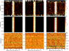 |
Fig. 5 2D maps of the intrinsic CCF profiles (top), their RMR model estimates (middle), and the residuals (bottom) for the three visits on 2021 March 24 (first column), 2022 July 03 (second column), and 2024 May 02 (third column). Dashed green lines mark the four transit contacts. Solid green line in the residual maps shows the best-fit global, model G1. |
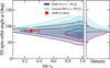 |
Fig. 6 Posterior distribution of the 3D spin–orbit angle ψ, derived by assuming a uniform prior on cos i⋆ (random stellar spin axis orientation). The purple and blue density contours represent the posterior distributions of ψ under the projected obliquity constraints from the RMR analysis and the classical RM analysis respectively, while the solid curves mark the 1, 2, and 3σ credible regions. The red point indicates the ψ value obtained from the RMR G2 fit. The side panel shows the 1D marginal posteriors of ψ. Both distributions consistently favor a polar orbital configuration. |
6 Discussion
Since the first detection of a Neptune on a polar orbit at the edge of the desert (i.e., in the recently identified ridge) by Bourrier et al. (2018) and the identification of a substantial fraction of polar orbits in the exoplanet population (Albrecht et al. 2021), subsequent studies (e.g., Bourrier et al. 2023; Attia et al. 2023; Castro-González et al. 2024a) have refined this view, suggesting that exo-Neptunes on polar orbits are preferentially found within the Neptunian ridge. The origin of polar orbits among ridge Neptunes has been investigated through various dynamical mechanisms. For example, the polar orbit of GJ 436 b ( ; Bourrier et al. 2022) can be explained by Kozai-Lidov cycles (Beust et al. 2012; Bourrier et al. 2018; Im et al. 2026). For GJ3470b (
 ; Stefànsson et al. 2022), possible mechanisms include Kozai–Lidov oscillations (Stefànsson et al. 2022) and disk-driven resonance (Petrovich et al. 2020; Stefànsson et al. 2022). For HAT-P-11 b (
 ; Bourrier et al. 2023), the proposed explanations include nodal precession (Yee et al. 2018), planet–planet scattering followed by Kozai–Lidov migration (Lu et al. 2025), and transition disk-driven resonance (Petrovich et al. 2020).
Our RMR analysis indicates that HAT-P-26 b is on a polar orbit ( ,
,  ). Two potential perturbers have been reported for this system. One is a stellar companion candidate (hereafter HAT-P-26 B;
  K), with a projected separation of less than 54 AU, as suggested by the spectral analysis (Piskorz et al. 2015). The other is an outer planetary companion (hereafter HAT-P-26 c), initially inferred from TTVs with an empirically preferred 2:1 mean-motion resonance (MMR), and since then hinted by a weak signal from the TESS light curve indicating a near 3:2 MMR (see Appendix F). In the following discussion, we first examined the current dynamical state in a framework of analytical secular Hamiltonian dynamics (Sect. 6.1). Then, we discussed possible migration scenarios, using the spin–orbit obliquity, planetary density, and envelope mass fraction (EMF) as joint constraints (Sect. 6.2).
6.1 Polar orbits as transitional states in secular Hamiltonian dynamics
It is well known that no analytical solution exists for the general four-body problem. However, when planets b and c are dynamically coupled in a rigid configuration, the long-term evolution of their common orbital plane can be analyzed. In this context, we investigated the formation of the polar orbit of HAT-P-26 b by analysing such a three-body problem following the formalism developed by Boué & Laskar (2006) and Boué & Fabrycky (2014).
Before performing the analysis, we first examined whether planets b and c are dynamically coupled, i.e., whether the ZLK timescale (τKoz) driven by HAT-P-26 B and the general relativistic timescale (τGR) induced by the host star exceed the precession period of the planetary system (τbc). We can follow Eqs. (44)–(46) in Boué & Fabrycky (2014) to calculate τKoz and τbc and derive τGR using Eq. (23) in Fabrycky & Tremaine (2007).
 (3)
(3)
 (4)
(4)
 (5)
(5)
Here, m, a, and e denote the mass, semimajor axis, and eccentricity, respectively, with the subscripts “⋆”, “b”, “c”, and “B” corresponding to the host star, the inner planet, the outer planet, and the stellar companion HAT-P-26 B. The adopted values for the host star and planet b are listed in Table 1. Using the orbital period of planet c (Pc = 6.59 days) reported by Dévora-Pajares et al. (2024), we derive a semimajor axis of ac = 0.063 AU. The bB represents the semiminor axis of the orbit of the outer stellar companion, defined as  . We adopt a companion mass of mB = 0.65 M⊙, consistent with an effective temperature of
  for a main sequence star, and assume a circular orbit (eB = 0). Since τbc ≪ τKoz and τGR, we conclude that the two planets are dynamically rigid. It should also be noted that, based on these timescales, the ZLK resonance induced by HAT-P-26 B has been suppressed by general relativity (see more discussion in Yee et al. 2018).
To analyze the dynamics in this system, we focus on the interactions among three angular momentum vectors: the stellar spin, the planetary orbit, and the companion’s orbit. Four characteristic precession frequencies were used to describe their relative influence: νPla/Star (the planetary orbit acting on the stellar spin); νStar/Pla (the stellar spin on the planetary orbit); νComp/Pla (the companion’s orbit on the planetary orbits); and νPla/Comp (the planetary orbits on the companion’s orbit). The direct interaction between the stellar spin and the companion’s orbit was neglected, since the associated quadrupole torque (∝m/a3) is weak due to the large orbital separation. The explicit frequency equations are not reproduced here. We refer interested readers to Sect. 3.2 of Boué & Fabrycky (2014) and Appendix A of Dalal et al. (2019) for precise model descriptions.
Since young stars are expected to rotate more rapidly and spin down over time due to magnetic braking, variations in stellar rotation should affect the precession frequencies of both the stellar spin axis and the planetary orbital plane. We therefore computed νPla/Star, vStar/Pla, νComp/Pla, and νComp/Pla as functions of the stellar rotation period, as illustrated in Fig. 7. During the fastrotation stage, (νPla/Star, νStar/Pla) ≫ (νComp/Pla, νComp), implying that the planetary orbits are dynamically coupled to the host star and that the perturbations from the outer stellar companion are negligible. As a result, the spin–orbit angle remains nearly constant during this phase. As the stellar spin gradually slows down, the system enters a transitional (hybrid) regime, (νPla/Star ~ νStar/Pla ~ νComp/Pla) ≫ νPla/Comp, corresponding to subplot (i) of Fig. 14 in Boué & Fabrycky (2014), in which only small spin–orbit angles are expected. Neither of these regimes can account for the observed polar orbit of planet b. Therefore, we only considered the remaining two scenarios: the Cassini state and the pure-orbital oscillation state.
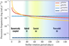 |
Fig. 7 Precession frequencies of vPla/Star (red), vStar/Pla (orange), vComp/Pla (cyan), and v>Pla/Comp (blue) as a function of the stellar rotation period. The background shading denotes different dynamical regimes: dynamically coupled (white), Hybrid (i) (green), Cassini (a) (yellow), and Pure orbit (b) (blue). The predicted 3D spin–orbit angles for regimes (i), (a), and (b) are given in Boué & Fabrycky (2014). |
6.1.1 Scenario 1: Cassini state
As shown in Fig. 7, since νStar/Pla decreases more steeply with the stellar rotation period than νPla/Star, the stellar spin has a negligible effect on the planetary orbital angular momentum. The planetary precession frequency (νComp/Pla) induced by the companion resonates with that of the star (νPla/Star), dominating the system’s dynamics and leading it into a classical Cassini state. Within this frame, the spin–orbit angle can reach a large value even with only a modest initial inclination of the outer stellar companion (see Fig. 14a in Boué & Fabrycky 2014).
The spin–orbit misalignments excited through Cassini states has been discussed in Correia (2015); Correia et al. (2016). The large misalignments require a decrease in the stellar rotation period triggered by tidal interactions (see Figs. 7 and 12 in Correia et al. 2016). In the absence of strong tidal interactions, the stellar spin evolution of HAT-P-26 is dominated by magnetic braking, leading to a monotonic spin-down. Under such conditions, capture into Cassini state 2 is prevented. While moderate obliquities may in principle be produced through Cassini state 1 during stellar spin-down, this mechanism cannot generate polar configurations (see also Fig. 7 in Correia et al. 2016). Therefore, while the Cassini state scenario cannot be ruled out, its ability to explain the observed polar orbit of planet b likely requires finetuned system parameters and should be tested with dedicated numerical simulations.
6.1.2 Scenario 2: Pure-orbit oscillation state
The system would be expected to finally settle into a pure-orbit regime (see Fig. 14b in Boué & Fabrycky 2014), in which the orbital plane of the planetary system oscillates about the system’s weighted-average angular momentum axis (i.e., the normal to the Laplace plane). Since the orbital angular momentum of the outer companion is much larger than that of planet b, the Laplace plane is nearly aligned with the companion’s orbital plane. If the initial inclination of the planetary plane was ib,t0 = 0° and that of HAT-P-26 B was  (i.e., ~40°), the spin-orbit angle would oscillate between 0° and 80°, periodically sweeping through the observed polar misalignment. The oscillation period is
  , indicating that this precession can operate efficiently within the system’s age (
 ; Hartman et al. 2011).
In summary, the stellar rotation period is poorly constrained, making it difficult to determine which scenario is favored. Nevertheless, a tentative resonance sweeping during the pure-orbital oscillation phase provides a plausible explanation for the polar orbit of HAT-P-26 b. We emphasize the following points: (i) The three-vector analysis is based on the assumption that the planets have small mutual inclinations and low eccentricities. If the planets are indeed in a MMR, both assumptions are naturally satisfied by the system’s long-term stability. (ii) If planet c orbits much farther from planet b (i.e., at ≳0.5 AU), the three-vector approximation may no longer be valid, and more detailed numerical simulations would be required to explore the dynamical behavior. (iii) Since the properties of planet c and the stellar companion remain poorly constrained, we cannot exclude other misalignment mechanisms discussed in the introduction, including primordial misalignment. A better constraint on the properties of planet c will be crucial for unveiling the system’s dynamical origin. In conclusion, under the hypothesis of a compact architecture, the polar orbit of HAT-P-26 b can be a temporary state during long-term pure orbital oscillations. However, it remains unclear whether this mechanism can account for the high occurrence of polar orbits observed in the Neptunian-ridge region.
6.2 Joint obliquity, eccentricity, density, and EMF as probes of migration history
6.2.1 DDM channel
Planetary density is thought to be a key parameter for the interplay between the orbital migration and atmospheric erosion of close-in Neptunes (Castro-González et al. 2024b; Bourrier et al. 2025). Fluffy (ρ<1 g/cm3) Neptunes might not evolve into dense ones (ρ > 1 g/cm3) through photo-evaporation during their late-stage evolution. Instead, they would arrive at their present-day locations by following different evolutionary pathways determined by their distinct primordial densities. Specifically, Bourrier et al. (2025) suggest that fluffy Neptunes (primarily found in the savanna region) tend to have nearly circular, well-aligned orbits, which provides potential evidence for DDM. In contrast, dense Neptunes are more likely to be driven by HEM towards the ridge and desert, leading to the emerging population of high eccentricity and misaligned orbits in these regions. In this line, fluffy DDM-migrated Neptunes are expected to be removed through evaporation at the shortest-period orbits within the ridge (Bourrier et al. 2025), and a similar outcome is expected for HEM-migrated fluffy Neptunes surviving disruption (Castro-González et al. 2026).
If DDM took place, HAT-P-26 b should have already lost a significant fraction of its atmosphere by its current age ( ; Hartman et al. 2011). However, the presence of prominent atmospheric H2O (Wakeford et al. 2017; MacDonald & Madhusudhan 2019; Panwar et al. 2022; A-thano et al. 2023; Ramos Rosado et al. 2025; Gressier et al. 2025), and SO2 (Gressier et al. 2025) features indicate that it still retains a substantial atmosphere, consistent with an EMF of about 26% estimated from interior models (see the bottom panel of Fig. 8, with values adopted from Acuña et al. 2024; Doyle et al. 2025). The DDM scenario is thus strongly disfavored, as it predicts almost complete atmospheric loss, inconsistent with the observed thick envelope. We conclude that even DDM combined with pure-orbital oscillations (Scenario 2) may reproduce the observed polar orbit, but they cannot readily account for the fluffy status of HAT-P-26 b at its present location near the density brink.
Furthermore, Doyle et al. (2025) found the EMF to increase linearly with planetary mass for Neptunes cooler than 1300 K (mostly in the ridge), and suggested that this relation is shaped by mass-dependent XUV-photoevaporation. Following the analysis by Doyle et al. (2025), we find HAT-P-26b (Teq ~ 1001 K) lies roughly 2σ above the linear model (see Fig. 8, bottom panel). There are three possible explanations for this higher value – a cloudy atmosphere can make the planet look larger than its real radius (Gao & Zhang 2020); additional internal heating make it expand (e.g., tidal heating; Bodenheimer et al. 2001; Ibgui & Burrows 2009; Millholland 2019; Ohmic dissipation Batygin & Stevenson 2010; Thorngren & Fortney 2018; Batygin 2025); and late (or recent) migration, which would leave the planets with larger EMFs than those that migrated earlier (e.g., Jackson et al. 2012; Howe & Burrows 2015; Luger et al. 2015; Owen & Lai 2018). Such late migration has also been suggested by Bourrier et al. (2025) to explain the fluffy planets observed across the brink and is consistent with the density filtering predicted by the tidal disruption formalism after HEM (Castro-González et al. 2026).
The question of whether HAT-P-26 b is cloud-free or possesses a high-altitude cloud deck remains unclear (Wakeford et al. 2017; MacDonald & Madhusudhan 2019; Panwar et al. 2022; A-thano et al. 2023; Ramos Rosado et al. 2025; Gressier et al. 2025). If a cloud deck exists at a pressure level of around 10−4 bar (Wakeford et al. 2017), the corresponding transit radius would be ~0.540RJ, which is about 13.7% larger than the 1-bar reference radius of 0.475 RJ. Therefore, the presence of a cloud deck could lead to a significant overestimation of the observed radius. Considering that the formation of clouds is typically sensitive to the atmospheric temperature, we therefore apply the color scale to the cooler planets (Teq < 1300 K) as shown in the bottom panel of Fig. 8. It is clear that planets with temperatures similar to HAT-P-26 b’s (Teq ~ 1000 K) follow the EMF–mass relation well, implying that clouds cannot account for the higher EMF of HAT-P-26 b. The other two possible explanations, internal heating and late migration, both occur during the evolution process. Therefore, the extremely low density (high EMF) within the Neptune population could serve as new clues, together with the spin–orbit obliquity and eccentricity, for constraining the formation pathway of this planet.
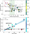 |
Fig. 8 Density distribution versus orbital period (top) and EMF versus planetary mass (bottom) for close-in Neptunes. In the top panel, all close-in Neptunes (3.5 R⊕ < Rp < 8.5R⊕, P < 30 days) are shown as grey dots with symbol size scaled to planetary radius. A subset with available 3D spin–orbit measurements is highlighted using distinct face colors, and planets on polar orbits (72°-108°) are emphasized in yellow. The Neptunian sample with EMF estimates from Doyle et al. (2025) is indicated by the blue and red boxes, as illustrated in the bottom panel. A dotted line marks the bulk-density level of 1 g cm−3, and the approximate brink boundary proposed by Bourrier et al. (2025) is shown as a dashed line. The ridge corresponds to the green-shaded region. In the bottom panel, the warmer Neptunes (Teff> 1300 K; red squares) have EMF values close to zero, indicating almost no surviving envelopes. While, the cooler sample (Teff ≤ 1300 K; gradient blue squares), as proposed by Doyle et al. (2025), follows the linear trend (solid blue line). Samples with only EMF upper limits are marked by triangles, and ridge planets are highlighted with light green outlines. |
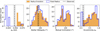 |
Fig. 9 Results from the N-body ZLK migration simulations of HAT-P-26 b. Left to right : semimajor axis, ab, stellar obliquity, ψAb, mutual inclination, ψbB, between the orbits of planet b and companion B, and the orbital eccentricity, eb. Dashed and dotted black lines mark the observed values and 1σ uncertainties. |
6.2.2 Coupled radius and HEM evolution
If the planet migrated to its current orbit after the host star’s UV/X-ray-bright phase (~100 Myr), its atmosphere would have avoided the most vigorous early-stage erosion (Bourrier et al. 2025; Owen & Lai 2018). HEM (hereafter scenario 3), specifically with high eccentricity driven by ZLK cycles followed by tidal circularization, is therefore the leading mechanism invoked for late-stage migration, as it explains the observed high obliquity and eccentric orbit.
The main challenge in the HEM scenario for the HAT-P-26 system is that ZLK oscillations are expected to operate efficiently only in single-planet systems. Basically, HEM and MMR cannot coexist as they drive nodal precession in opposite directions and MMR configurations are extremely fragile at large eccentricities (e.g., Terquem & Papaloizou 2007; Izidoro et al. 2017; Petit et al. 2017; Leleu et al. 2021). Even if the planets are not locked in an MMR, the presence of a nearby planet c would enhance the apsidal precession rate of planet b through planet–planet interactions, thereby suppressing or breaking the ZLK cycles. Does planet c exist, and if so, is it in an MMR? We find that the proposed MMR configuration of the planet candidate inferred from TTV residuals is inconsistent with that derived from the TESS light curve analysis (see Appendix F). Furthermore, using the TTVs reported in A-thano et al. (2023), we carried out a TTV inversion with TTVFast (Deck et al. 2014; Sun et al. 2025), but found no significant evidence for planet c (see Appendix F for details). Overall, the evidence for planet c remains inconclusive. If planet c is confirmed and found to be in an MMR configuration by future observations, the planets were most likely locked into MMR in the early DDM phase, during which planet b would have experienced strong photoevaporative stripping. To retain its observed high EMF, it should either initially host an extremely massive envelope or have experienced significant radius inflation through tidal or ohmic dissipation. Nevertheless, it remains a challenge to explain how the polar orbit formed in the DDM scenario.
Given the inconclusive evidence for planet c, we did not include it in our HEM model. We treated the system as a hierarchical triple consisting of the host star, planet b, and the wide stellar companion HAT-P-26 B (MB = 0.65 M⊙, aB = 54 AU, eB = 0). Following Lu et al. (2025), we employed a coupled ZLK-evolution and radius-inflation framework to assess whether this configuration can account for the observed obliquity, eccentricity, and low density of planet b. We integrated the three-body system using the IAS15 integrator in REBOUND (Rein & Liu 2012), with REBOUNDx (Tamayo et al. 2020) providing general relativistic (gr; Anderson et al. 1975) apsidal precession and tides_spin evolution (Lu et al. 2023) for the planet. We adopted a constant time lag tidal model and an accelerated lag τ = 10−5 yr (see Sect. 3.4 in Lu et al. 2025 for details). The integration proceeds for 5 Myr and terminates early upon reaching eb < 0.12 (see Table C.1) or collision. We performed two sets of simulations for HAT-P-26 b, each adopting a different treatment of the planetary radius. The detailed settings and results (see Fig. 9) are shown below:
Case 1: fixed observed radius. We assume the observed present-day radius of HAT-P-26 b (Rp = 6.33 R⊕; Hartman et al. 2011), held constant throughout the integration. The dynamic coupling between tidal heating and the radius is neglected. In this case, 18% of all simulated systems migrate inward to a < 0.1 AU, with 16% successfully reaching eb < 0.12 (the remaining 2 systems reach a < 0.1 AU but retain eb > 0.12). The stellar obliquity distribution peaks near 90°, with 38% of successfully migrated systems (eb < 0.12) having ψAb ∈ [60°, 120°], consistent with the observed polar orbit of HAT-P-26 b. However, the migrated systems preferentially settle at a ≈ 0.015-0.03 AU, systematically undershooting the observed value of 0.047 AU. This occurs because the static tidal precession at 6.33 R⊕ is insufficient to quench ZLK oscillations at the observed semimajor axis, and the ZLK cycle persists until GR precession ( ), which grows steeply at small a, ultimately suppresses the eccentricity oscillations at a < aobs.
Case 2: radius evolution with dynamic coupling. The radius is self-consistently coupled to the tidal heating rate using the MESA thermal evolution tracks from Millholland et al. (2020). During high-eccentricity phases of ZLK oscillations, the planet inflates in response to intense tidal dissipation at close pericenter passages, with the radius determined by interpolating the MESA grid as a function of tidal luminosity (Lu et al. 2025, Eq. (13)). Of all simulated systems, ~18% migrate inward to a < 0.1 AU, and the obliquity distribution is similarly peaked near 90°. However, no migrated systems reach the observed eccentricity within the integration time, retaining ēb ≈ 0.28 at semimajor axes that all exceed the observed value. During high-eccentricity epochs, tidal heating inflates the planet substantially, enhancing the tidal precession rate by up to (Rinfl/Robs)5. This causes ZLK oscillations to be quenched prematurely, at a larger semimajor axis, before the orbit has decayed sufficiently to reach the observed configuration. The planet is effectively stranded on a wider, still-eccentric orbit.
The two cases demonstrate that the thermal response of the planet’s envelope is dynamically significant, as proposed by Lu et al. (2025). A static radius (Case 1) allows for migration and tidal damping to low eccentricity, but overshoots the target orbit. This is because GR precession, rather than tidal precession, ultimately quenches the ZLK cycle at short periods. When the radius responds dynamically to tidal heating (Case 2), enhanced tidal precession quenches ZLK oscillations at wider orbits before the eccentricity has damped to the observed level. Neither of our two idealized cases exactly reproduces the observed orbit of HAT-P-26 b, which is expected given that we have not attempted to fine-tune the multidimensional parameter space (initial semimajor axis, tidal quality factor, Love number, mutual inclination, and internal composition; see Lu et al. 2025, Sect. 4). We also caution that extracting this information in practice faces several challenges. First, the MESA luminosity–radius relation shows considerable scatter, which may systematically overestimate the degree of inflation in our population synthesis and thereby amplify the premature quenching of ZLK oscillations. Second, atmospheric mass loss driven by photoevaporation (e.g., Vissapragada et al. 2022) modifies the EMF over Gyr timescales and should be accounted for. We therefore emphasize that the present analysis provides only a simplified exploration of the ZLK mechanism, as it does not account for mass loss. In a more comprehensive follow-up study, we plan to use the jade11 code (Attia et al. 2021, 2025) to place tighter constraints on the late-stage migratory evolution of HAT-P-26 b.
7 Conclusion
We obtained a polar orbit for HAT-P-26 b ( ,
,  ) by employing the RMR technique to analyze the RM effect, using data from three ESPRESSO visits collated from the ATREIDES collaboration. Our analysis leads to the following key conclusions:
We identified HAT-P-26 b as a new member of the planets on eccentric and polar orbits in the Neptunian ridge, alongside GJ 436 b, HAT-P-11 b, and GJ 3470 b;
The observed polar orbit may represent a transient configuration produced by pure-orbital oscillations (scenario 2) driven by a sufficiently inclined stellar companion. HEM (scenario 3) could also have shaped the orbital architecture in the past. Both scenarios can be further tested and constrained by investigating the existence of planet c;
The low density (high EMF) of HAT-P-26 b might arise from the competition between photoevaporation and atmospheric inflation. An apparently enlarged radius caused by clouds can be ruled out, since other ridge Neptunes with comparable equilibrium temperatures do not show elevated EMFs.
As a next step, we plan to confirm (or rule out) the existence of the potential HAT-P-26 c and the stellar companion with the help of, for instance, the ongoing long-term CORALIE (Queloz et al. 2000; Udry et al. 2000) monitoring. We will then perform follow-up analyses of the transmission spectra to better characterize the atmosphere, followed by simulations of the coupled dynamical and atmospheric evolution using the JADE code11 (Attia et al. 2021, 2025) to provide a more realistic picture of the orbital migration pathways of HAT-P-26 b. This work is part of the ATREIDES collaboration (Bourrier et al. 2025), aimed at measuring the 3D orbital architectures of ~60 exo-Neptunes and rewinding their joint atmospheric and orbital history to shed new light on the origins of the close-in Neptunian exoplanets. In the wake of ATREIDES, other surveys are now contributing to expand the orbital architecture sample of exo-Neptunes (e.g., Espinoza-Retamal et al. 2026) and to investigate the proposed bimodality between polar ridge orbits and aligned savanna orbits that would arise from HEM and DDM (Bourrier et al. 2025).
Data availability
We added our results for the HAT-P-26 system to the ATREIDES catalog, publicly available on the DACE platform at https://doi.org/10.82180/dace-uz7tjl61. This catalog stores key stellar and planetary properties, including our revised ephemeris to enable follow-up observations, as well as ANTARES S homogeneous spectroscopic data products. The DACE platform is available at https://dace.unige.ch.
Acknowledgements
We are grateful to the anonymous referee for their valuable comments, which significantly improved this work. This project has received funding from the European Research Council (ERC) under the European Union’s Horizon 2020 research and innovation programme (project Spice Dune, grant agreement No 947634). This work has been carried out in the frame of the National Centre for Competence in Research PlanetS supported by the Swiss National Science Foundation (SNSF) under grants 51NF40_182901 and 51NF40_205606. This research made use of the open source Python package exoctk, the Exoplanet Characterization Toolkit (Bourque et al. 2021). X.L. acknowledges support from the Natural Science Foundation Youth Program of Sichuan Province (Grant No. 2024NSFSC1363), the Doctoral Initiation Fund of China West Normal University (Grant No. 22kE036), and the Sino-German (CSC-DAAD) Postdoc Scholarship Program (Grant No. 57678375), funded by the China Scholarship Council and the German Academic Exchange Service. MRZO acknowledges financial support by the Spanish Ministerio de Ciencia, Innovación y Universidades through project PID2022-137241NB-C42. ACMC acknowledges support from FCT – Fundação para a Ciência e a Tecnologia, I.P., Portugal, through the CFisUC project UID/04564/2025 (with DOI identifier 10.54499/UID/04564/2025). EDM acknowledges the support by the project MICIU/AEI/PID2023-150468NB-I00 and by the Ramón y Cajal contract RyC2022-035854-I funded by the Spanish MICIU/AEI/10.13039/501100011033 and by ESF+. V.A. acknowledges support from FCT – Fundação para a Ciência e Tecnologia through national funds and from FEDER via COM-PETE2020 – Programa Operacional Competitividade e Internacionalização, under the grants UIDB/04434/2020 (DOI: 10.54499/UIDB/04434/2020) and UIDP/04434/2020 (DOI: 10.54499/UIDP/04434/2020), as well as through a work contract funded by the FCT Scientific Employment Stimulus program (reference 2023.06055.CEECIND/CP2839/CT0005, DOI: 10.54499/2023.06055.CEECIND/CP2839/CT0005). L.S. acknowledges financial support from the National Natural Science Foundation of China (grant numbers 12003063). L.S. also acknowledges support from International Centre of Supernovae, Yunnan Key Laboratory (grant number 202302AN360001). This work is based in part on data collected under the NGTS project at the ESO La Silla Paranal Observatory. The NGTS facility is operated by a consortium institutes with support from the UK Science and Technology Facilities Council (STFC) under projects ST/M001962/1, ST/S002642/1 and ST/W003163/1. F.H. gratefully acknowledges continued support from the NGTS consortium, and the financial support of the Rugby School Group, whose employment enables their ongoing contribution to astronomical research. This work was funded by the European Union (ERC, FIERCE, 101052347). Views and opinions expressed are however those of the author(s) only and do not necessarily reflect those of the European Union or the European Research Council. Neither the European Union nor the granting authority can be held responsible for them. This work was also supported by FCT – Fundação para a Ciência e a Tecnologia through national funds by this grant: UID/04434/2025. This research was part funded by the UKRI (Grants ST/X001121/1). This work has made use of data from the European Space Agency (ESA) mission Gaia (https://www.cosmos.esa.int/gaia), processed by the Gaia Data Processing and Analysis Consortium (DPAC, https://www.cosmos.esa.int/web/gaia/dpac/consortium). Funding for the DPAC has been provided by national institutions, in particular the institutions participating in the Gaia Multilateral Agreement. We acknowledge financial support from the Agencia Estatal de Investigación of the Ministerio de Ciencia e Innovación MCIN/AEI/10.13039/501100011033 and the ERDF “A way of making Europe” through project PID2024-158486OB-C32. This work is in part funded with a UKRI Future Leader Fellowship grant numbers MR/S035214/1 and MR/Y011759/1. J.I.G.H. acknowledges financial support from the Spanish Ministry of Science, Innovation and Universities (MICIU) project PID2023-149982NB-I00. M.P.B. gratefully acknowledges support from UK Research and Innovation (UKRI) under the UK government’s Horizon Europe funding guarantee for an ERC starting grant [grant number EP/Z000890/1] N.L. acknowledges the support of the UD Annie Jump Cannon Fund PHYS462112 R.A. acknowledges the Swiss National Science Foundation (SNSF) support under the Post-Doc Mobility grant P500PT_222212 and the support of the Institut Trottier de Recherche sur les Exoplanètes (IREx). This work has been carried out within the framework of the National Centre of Competence in Research PlanetS supported by the Swiss National Science Foundation. The authors acknowledge the financial support of the SNSF. S.J.M. acknowledges support from the Massachusetts Institute of Technology through the Desmond Fellowship.
References
- A-thano, N., Awiphan, S., Jiang, I.-G., et al. 2023, AJ, 166, 223 [CrossRef] [Google Scholar]
- Acuña, L., Kreidberg, L., Zhai, M., & Mollière, P. 2024, A&A, 688, A60 [NASA ADS] [CrossRef] [EDP Sciences] [Google Scholar]
- Adibekyan, V. Z., Santos, N. C., Sousa, S. G., & Israelian, G. 2011, A&A, 535, L11 [NASA ADS] [CrossRef] [EDP Sciences] [Google Scholar]
- Adibekyan, V., Delgado-Mena, E., Figueira, P., et al. 2016, A&A, 591, A34 [NASA ADS] [CrossRef] [EDP Sciences] [Google Scholar]
- Albrecht, S. H., Marcussen, M. L., Winn, J. N., Dawson, R. I., & Knudstrup, E. 2021, ApJ, 916, L1 [NASA ADS] [CrossRef] [Google Scholar]
- Albrecht, S. H., Dawson, R. I., & Winn, J. N. 2022, PASP, 134, 082001 [NASA ADS] [CrossRef] [Google Scholar]
- Allart, R., Bourrier, V., Lovis, C., et al. 2018, Science, 362, 1384 [Google Scholar]
- Allart, R., Lovis, C., Faria, J., et al. 2022, A&A, 666, A196 [NASA ADS] [CrossRef] [EDP Sciences] [Google Scholar]
- Ambikasaran, S., Foreman-Mackey, D., Greengard, L., Hogg, D. W., & O’Neil, M. 2015, IEEE Trans. Pattern Anal. Mach. Intell., 38, 252 [Google Scholar]
- Anderson, J. D., Esposito, P. B., Martin, W., Thornton, C. L., & Muhleman, D. O. 1975, ApJ, 200, 221 [NASA ADS] [CrossRef] [Google Scholar]
- Attia, M., Bourrier, V., Eggenberger, P., et al. 2021, A&A, 647, A40 [NASA ADS] [CrossRef] [EDP Sciences] [Google Scholar]
- Attia, M., Bourrier, V., Delisle, J.-B., & Eggenberger, P. 2023, A&A, 674, A120 [NASA ADS] [CrossRef] [EDP Sciences] [Google Scholar]
- Attia, M., Bourrier, V., Bolmont, E., et al. 2025, A&A, 702, A132 [NASA ADS] [CrossRef] [EDP Sciences] [Google Scholar]
- Bate, M. R. 2018, MNRAS, 475, 5618 [Google Scholar]
- Bate, M. R., Lodato, G., & Pringle, J. E. 2010, MNRAS, 401, 1505 [NASA ADS] [CrossRef] [Google Scholar]
- Batygin, K. 2012, Nature, 491, 418 [NASA ADS] [CrossRef] [Google Scholar]
- Batygin, K. 2025, ApJ, 985, 87 [Google Scholar]
- Batygin, K., & Stevenson, D. J. 2010, ApJ, 714, L238 [NASA ADS] [CrossRef] [Google Scholar]
- Beust, H., Bonfils, X., Montagnier, G., Delfosse, X., & Forveille, T. 2012, A&A, 545, A88 [NASA ADS] [CrossRef] [EDP Sciences] [Google Scholar]
- Biazzo, K., D’Orazi, V., Desidera, S., et al. 2022, A&A, 664, A161 [NASA ADS] [CrossRef] [EDP Sciences] [Google Scholar]
- Biddle, L. I., Bowler, B. P., Morgan, M., Tran, Q. H., & Wu, Y.-L. 2025, Nature, 644, 356 [Google Scholar]
- Bodenheimer, P., Lin, D. N. C., & Mardling, R. A. 2001, ApJ, 548, 466 [NASA ADS] [CrossRef] [Google Scholar]
- Boué, G., & Fabrycky, D. C. 2014, ApJ, 789, 111 [CrossRef] [Google Scholar]
- Boué, G., & Laskar, J. 2006, Icarus, 185, 312 [Google Scholar]
- Boué, G., Montalto, M., Boisse, I., Oshagh, M., & Santos, N. C. 2013, A&A, 550, A53 [NASA ADS] [CrossRef] [EDP Sciences] [Google Scholar]
- Bourque, M., Espinoza, N., Filippazzo, J., et al. 2021, The Exoplanet Characterization Toolkit (ExoCTK) [Google Scholar]
- Bourrier, V., Cegla, H. M., Lovis, C., & Wyttenbach, A. 2017, A&A, 599, A33 [NASA ADS] [CrossRef] [EDP Sciences] [Google Scholar]
- Bourrier, V., Lovis, C., Beust, H., et al. 2018, Nature, 553, 477 [NASA ADS] [CrossRef] [Google Scholar]
- Bourrier, V., Lovis, C., Cretignier, M., et al. 2021, A&A, 654, A152 [NASA ADS] [CrossRef] [EDP Sciences] [Google Scholar]
- Bourrier, V., Deline, A., Krenn, A., et al. 2022, A&A, 668, A31 [NASA ADS] [CrossRef] [EDP Sciences] [Google Scholar]
- Bourrier, V., Attia, M., Mallonn, M., et al. 2023, A&A, 669, A63 [NASA ADS] [CrossRef] [EDP Sciences] [Google Scholar]
- Bourrier, V., Delisle, J.-B., Lovis, C., et al. 2024, A&A, 691, A113 [NASA ADS] [CrossRef] [EDP Sciences] [Google Scholar]
- Bourrier, V., Steiner, M., Castro-González, A., et al. 2025, A&A, 701, A190 [NASA ADS] [CrossRef] [EDP Sciences] [Google Scholar]
- Bruntt, H., Bedding, T. R., Quirion, P.-O., et al. 2010, MNRAS, 405, 1907 [NASA ADS] [Google Scholar]
- Bryant, E. M., Bayliss, D., McCormac, J., et al. 2020, MNRAS, 494, 5872 [Google Scholar]
- Castro-González, A., Demangeon, O. D. S., Lillo-Box, J., et al. 2023, A&A, 675, A52 [NASA ADS] [CrossRef] [EDP Sciences] [Google Scholar]
- Castro-González, A., Bourrier, V., Lillo-Box, J., et al. 2024a, A&A, 689, A250 [NASA ADS] [CrossRef] [EDP Sciences] [Google Scholar]
- Castro-González, A., Lillo-Box, J., Armstrong, D. J., et al. 2024b, A&A, 691, A233 [NASA ADS] [CrossRef] [EDP Sciences] [Google Scholar]
- Castro-González, A., Bouchy, F., Correia, A. C. M., et al. 2025, A&A, 699, A344 [Google Scholar]
- Castro-González, A., Bourrier, V., Ehrenreich, D., et al. 2026, A&A, 709, L17 [NASA ADS] [CrossRef] [EDP Sciences] [Google Scholar]
- Cavallini, F., Ceppatelli, G., & Righini, A. 1985, A&A, 150, 256 [NASA ADS] [Google Scholar]
- Cegla, H. M., Lovis, C., Bourrier, V., et al. 2016, A&A, 588, A127 [NASA ADS] [CrossRef] [EDP Sciences] [Google Scholar]
- Chatterjee, S., Ford, E. B., Matsumura, S., & Rasio, F. A. 2008, ApJ, 686, 580 [NASA ADS] [CrossRef] [Google Scholar]
- Correia, A. C. M. 2015, A&A, 582, A69 [NASA ADS] [CrossRef] [EDP Sciences] [Google Scholar]
- Correia, A. C. M., Boué, G., & Laskar, J. 2016, Celest. Mech. Dyn. Astron., 126, 189 [NASA ADS] [CrossRef] [Google Scholar]
- Correia, A. C. M., Bourrier, V., & Delisle, J.-B. 2020, A&A, 635, A37 [NASA ADS] [CrossRef] [EDP Sciences] [Google Scholar]
- Cretignier, M., Dumusque, X., Allart, R., Pepe, F., & Lovis, C. 2020, A&A, 633, A76 [NASA ADS] [CrossRef] [EDP Sciences] [Google Scholar]
- Dalal, S., Hébrard, G., Lecavelier des Étangs, A., et al. 2019, A&A, 631, A28 [NASA ADS] [CrossRef] [EDP Sciences] [Google Scholar]
- Davis, T. A., & Wheatley, P. J. 2009, MNRAS, 396, 1012 [CrossRef] [Google Scholar]
- Dawson, R. I., & Johnson, J. A. 2018, ARA&A, 56, 175 [NASA ADS] [CrossRef] [Google Scholar]
- Deck, K. M., Agol, E., Holman, M. J., & Nesvorný, D. 2014, ApJ, 787, 132 [CrossRef] [Google Scholar]
- Delgado Mena, E., Tsantaki, M., Adibekyan, V. Z., et al. 2017, A&A, 606, A94 [NASA ADS] [CrossRef] [EDP Sciences] [Google Scholar]
- Delgado Mena, E., Moya, A., Adibekyan, V., et al. 2019, A&A, 624, A78 [NASA ADS] [CrossRef] [EDP Sciences] [Google Scholar]
- Delisle, J.-B., Unger, N., Hara, N. C., & Ségransan, D. 2022, A&A, 659, A182 [NASA ADS] [CrossRef] [EDP Sciences] [Google Scholar]
- Dévora-Pajares, M., Pozuelos, F. J., Thuillier, A., et al. 2024, MNRAS, 532, 4752 [CrossRef] [Google Scholar]
- Doyle, A. P., Davies, G. R., Smalley, B., Chaplin, W. J., & Elsworth, Y. 2014, MNRAS, 444, 3592 [Google Scholar]
- Doyle, L., Armstrong, D. J., Acuña, L., et al. 2025, MNRAS, 539, 3138 [Google Scholar]
- Eaton, J. A., Henry, G. W., & Fekel, F. C. 2003, in Astrophysics and Space Science Library, 288, Astrophysics and Space Science Library, ed. T. D. Oswalt, 189 [Google Scholar]
- Ehrenreich, D., Bourrier, V., Wheatley, P. J., et al. 2015, Nature, 522, 459 [Google Scholar]
- Espinoza-Retamal, J. I., Stefánsson, G., Petrovich, C., et al. 2024, AJ, 168, 185 [Google Scholar]
- Espinoza-Retamal, J. I., Winn, J. N., Brahm, R., et al. 2026, AJ, accepted [arXiv:2602.18553] [Google Scholar]
- Fabrycky, D., & Tremaine, S. 2007, ApJ, 669, 1298 [NASA ADS] [CrossRef] [Google Scholar]
- Fabrycky, D. C., Lissauer, J. J., Ragozzine, D., et al. 2014, ApJ, 790, 146 [Google Scholar]
- Faria, J. P., Haywood, R. D., Brewer, B. J., et al. 2016, A&A, 588, A31 [NASA ADS] [CrossRef] [EDP Sciences] [Google Scholar]
- Feinstein, A. D., Montet, B. T., Johnson, M. C., et al. 2021, AJ, 162, 213 [NASA ADS] [CrossRef] [Google Scholar]
- Foreman-Mackey, D., Hogg, D. W., Lang, D., & Goodman, J. 2013, PASP, 125, 306 [Google Scholar]
- Frazier, R. C., Stefánsson, G., Mahadevan, S., et al. 2023, ApJ, 944, L41 [NASA ADS] [CrossRef] [Google Scholar]
- Gaia Collaboration (Brown, A. G. A., et al.) 2018, A&A, 616, A1 [NASA ADS] [CrossRef] [EDP Sciences] [Google Scholar]
- Gaia Collaboration (Vallenari, A., et al.) 2023, A&A, 674, A1 [NASA ADS] [CrossRef] [EDP Sciences] [Google Scholar]
- Gao, P., & Zhang, X. 2020, ApJ, 890, 93 [Google Scholar]
- Goldreich, P., & Tremaine, S. 1979, ApJ, 233, 857 [Google Scholar]
- Gomes da Silva, J., Figueira, P., Santos, N., & Faria, J. 2018, J. Open Source Softw., 3, 667 [Google Scholar]
- Gomes da Silva, J., Santos, N. C., Adibekyan, V., et al. 2021, A&A, 646, A77 [NASA ADS] [CrossRef] [EDP Sciences] [Google Scholar]
- Gressier, A., Batalha, N. E., Wogan, N., et al. 2025, AJ, 170, 292 [Google Scholar]
- Handley, L. B., Howard, A. W., Rubenzahl, R. A., et al. 2025, AJ, 169, 212 [Google Scholar]
- Hartman, J. D., Bakos, G. Á., Kipping, D. M., et al. 2011, ApJ, 728, 138 [NASA ADS] [CrossRef] [Google Scholar]
- Hjorth, M., Albrecht, S., Hirano, T., et al. 2021, PNAS, 118, e2017418118 [NASA ADS] [CrossRef] [Google Scholar]
- Howe, A. R., & Burrows, A. 2015, ApJ, 808, 150 [NASA ADS] [CrossRef] [Google Scholar]
- Husser, T.-O., Wende-von Berg, S., Dreizler, S., et al. 2013, A&A, 553, A6 [NASA ADS] [CrossRef] [EDP Sciences] [Google Scholar]
- Ibgui, L., & Burrows, A. 2009, ApJ, 700, 1921 [Google Scholar]
- Im, H., Lu, T., Rice, M., et al. 2026, ApJ, 1003, 84 [Google Scholar]
- Izidoro, A., Ogihara, M., Raymond, S. N., et al. 2017, MNRAS, 470, 1750 [Google Scholar]
- Jackson, B., Greenberg, R., & Barnes, R. 2008, ApJ, 681, 1631 [NASA ADS] [CrossRef] [Google Scholar]
- Jackson, A. P., Davis, T. A., & Wheatley, P. J. 2012, MNRAS, 422, 2024 [Google Scholar]
- Kipping, D. M. 2013, MNRAS, 435, 2152 [Google Scholar]
- Knudstrup, E., Albrecht, S. H., Winn, J. N., et al. 2024, A&A, 690, A379 [NASA ADS] [CrossRef] [EDP Sciences] [Google Scholar]
- Kokori, A., Tsiaras, A., Edwards, B., et al. 2023, ApJS, 265, 4 [NASA ADS] [CrossRef] [Google Scholar]
- Kozai, Y. 1962, AJ, 67, 591 [Google Scholar]
- Kreidberg, L. 2015, PASP, 127, 1161 [Google Scholar]
- Kurucz, R. L. 1993, SYNTHE spectrum synthesis programs and line data [Google Scholar]
- Lai, D. 2012, MNRAS, 423, 486 [NASA ADS] [CrossRef] [Google Scholar]
- Lai, D., Foucart, F., & Lin, D. N. C. 2011, MNRAS, 412, 2790 [NASA ADS] [CrossRef] [Google Scholar]
- Lecavelier Des Etangs, A. 2007, A&A, 461, 1185 [NASA ADS] [CrossRef] [EDP Sciences] [Google Scholar]
- Leconte, J., Chabrier, G., Baraffe, I., & Levrard, B. 2010, A&A, 516, A64 [NASA ADS] [CrossRef] [EDP Sciences] [Google Scholar]
- Leleu, A., Alibert, Y., Hara, N. C., et al. 2021, A&A, 649, A26 [NASA ADS] [CrossRef] [EDP Sciences] [Google Scholar]
- Lidov, M. L. 1962, Planet. Space Sci., 9, 719 [Google Scholar]
- Lin, D. N. C., Bodenheimer, P., & Richardson, D. C. 1996, Nature, 380, 606 [Google Scholar]
- Löhner-Böttcher, J., Schmidt, W., Schlichenmaier, R., Steinmetz, T., & Holzwarth, R. 2019, A&A, 624, A57 [Google Scholar]
- Louden, E. M., & Millholland, S. C. 2024, ApJ, 974, 304 [Google Scholar]
- Lu, T., Rein, H., Tamayo, D., et al. 2023, ApJ, 948, 41 [NASA ADS] [CrossRef] [Google Scholar]
- Lu, T., An, Q., Li, G., et al. 2025, ApJ, 979, 218 [Google Scholar]
- Luger, R., Barnes, R., Lopez, E., et al. 2015, Astrobiology, 15, 57 [Google Scholar]
- Lundkvist, M. S., Kjeldsen, H., Albrecht, S., et al. 2016, Nat. Commun., 7, 11201 [Google Scholar]
- MacDonald, R. J., & Madhusudhan, N. 2019, MNRAS, 486, 1292 [Google Scholar]
- Mamajek, E. E., & Hillenbrand, L. A. 2008, ApJ, 687, 1264 [Google Scholar]
- Mancini, L., Esposito, M., Covino, E., et al. 2022, A&A, 664, A162 [NASA ADS] [CrossRef] [EDP Sciences] [Google Scholar]
- Mazeh, T., Zucker, S., & Pont, F. 2005, MNRAS, 356, 955 [NASA ADS] [CrossRef] [Google Scholar]
- Mazeh, T., Holczer, T., & Faigler, S. 2016, A&A, 589, A75 [NASA ADS] [CrossRef] [EDP Sciences] [Google Scholar]
- McLaughlin, D. B. 1924, ApJ, 60, 22 [Google Scholar]
- McQuillan, A., Mazeh, T., & Aigrain, S. 2014, ApJS, 211, 24 [Google Scholar]
- Millholland, S. 2019, ApJ, 886, 72 [NASA ADS] [CrossRef] [Google Scholar]
- Millholland, S., Petigura, E., & Batygin, K. 2020, ApJ, 897, 7 [NASA ADS] [CrossRef] [Google Scholar]
- Naoz, S., Farr, W. M., Lithwick, Y., Rasio, F. A., & Teyssandier, J. 2011, Nature, 473, 187 [NASA ADS] [CrossRef] [Google Scholar]
- Nesvorný, D., Kipping, D., Terrell, D., et al. 2013, ApJ, 777, 3 [CrossRef] [Google Scholar]
- Noyes, R. W., Hartmann, L. W., Baliunas, S. L., Duncan, D. K., & Vaughan, A. H. 1984, ApJ, 279, 763 [Google Scholar]
- Orell-Miquel, J., Sampson, K., Morley, C. V., et al. 2026, AJ, 171, 194 [Google Scholar]
- Owen, J. E., & Jackson, A. P. 2012, MNRAS, 425, 2931 [Google Scholar]
- Owen, J. E., & Lai, D. 2018, MNRAS, 479, 5012 [Google Scholar]
- Owen, J. E., & Wu, Y. 2013, ApJ, 775, 105 [Google Scholar]
- Panwar, V., Désert, J.-M., Todorov, K. O., et al. 2022, MNRAS, 510, 3236 [CrossRef] [Google Scholar]
- Parviainen, H., & Aigrain, S. 2015, MNRAS, 453, 3821 [Google Scholar]
- Pepe, F., Cristiani, S., Rebolo, R., et al. 2021, A&A, 645, A96 [NASA ADS] [CrossRef] [EDP Sciences] [Google Scholar]
- Petit, A. C., Laskar, J., & Boué, G. 2017, A&A, 607, A35 [NASA ADS] [CrossRef] [EDP Sciences] [Google Scholar]
- Petrovich, C., Muñoz, D. J., Kratter, K. M., & Malhotra, R. 2020, ApJ, 902, L5 [NASA ADS] [CrossRef] [Google Scholar]
- Piskorz, D., Knutson, H. A., Ngo, H., et al. 2015, ApJ, 814, 148 [Google Scholar]
- Queloz, D., Mayor, M., Weber, L., et al. 2000, A&A, 354, 99 [NASA ADS] [Google Scholar]
- Radzom, B. T., Dong, J., Rice, M., et al. 2024, AJ, 168, 116 [Google Scholar]
- Ramos Rosado, L. M., Sing, D. K., Allen, N. H., et al. 2025, AJ, 169, 259 [Google Scholar]
- Rasmussen, C. E. & Williams, C. K. I. 2006, Gaussian Processes for Machine Learning [Google Scholar]
- Rein, H., & Liu, S.-F. 2012, A&A, 537, A128 [NASA ADS] [CrossRef] [EDP Sciences] [Google Scholar]
- Roberts, S., Osborne, M., Ebden, M., et al. 2012, Philos. Transa. Roy. Soc. Lond. A, 371, 20110550 [Google Scholar]
- Rossiter, R. A. 1924, ApJ, 60, 15 [Google Scholar]
- Rothman, L. S., Gordon, I. E., Babikov, Y., et al. 2013, J. Quant. Spec. Radiat. Transf., 130, 4 [NASA ADS] [CrossRef] [Google Scholar]
- Sethi, R., & Millholland, S. C. 2025, ApJ, 988, 247 [Google Scholar]
- Sing, D. K., Wakeford, H. R., Showman, A. P., et al. 2015, MNRAS, 446, 2428 [NASA ADS] [CrossRef] [Google Scholar]
- Sing, D. K., Rustamkulov, Z., Thorngren, D. P., et al. 2024, Nature, 630, 831 [NASA ADS] [CrossRef] [Google Scholar]
- Smith, A. M. S., Eigmüller, P., Gurumoorthy, R., et al. 2020, Astron. Nachr., 341, 273 [Google Scholar]
- Sousa, S. G., Adibekyan, V., Delgado-Mena, E., et al. 2021, A&A, 656, A53 [NASA ADS] [CrossRef] [EDP Sciences] [Google Scholar]
- Speagle, J. S. 2020, MNRAS, 493, 3132 [Google Scholar]
- Stefànsson, G., Mahadevan, S., Petrovich, C., et al. 2022, ApJ, 931, L15 [NASA ADS] [CrossRef] [Google Scholar]
- Stevenson, K. B., Bean, J. L., Seifahrt, A., et al. 2016, ApJ, 817, 141 [NASA ADS] [CrossRef] [Google Scholar]
- Suárez Mascareño, A., Rebolo, R., & González Hernández, J. I. 2016, A&A, 595, A12 [Google Scholar]
- Sun, L., Gu, S., Wang, X., et al. 2025, Nat. Astron., 9, 1184 [Google Scholar]
- Szabó, G. M., & Kiss, L. L. 2011, ApJ, 727, L44 [Google Scholar]
- Tamayo, D., Rein, H., Shi, P., & Hernandez, D. M. 2020, MNRAS, 491, 2885 [NASA ADS] [CrossRef] [Google Scholar]
- Terquem, C., & Papaloizou, J. C. B. 2007, ApJ, 654, 1110 [Google Scholar]
- Thorngren, D. P., & Fortney, J. J. 2018, AJ, 155, 214 [Google Scholar]
- Triaud, A. H. M. J. 2018, in Handbook of Exoplanets, eds. H. J. Deeg, & J. A. Belmonte, 2 [Google Scholar]
- Udry, S., Mayor, M., Naef, D., et al. 2000, A&A, 356, 590 [NASA ADS] [Google Scholar]
- Valenti, J. A., & Fischer, D. A. 2005, ApJS, 159, 141 [Google Scholar]
- Vaughan, A. H., & Preston, G. W. 1980, PASP, 92, 385 [Google Scholar]
- Vaughan, A. H., Preston, G. W., & Wilson, O. C. 1978, PASP, 90, 267 [Google Scholar]
- Vissapragada, S., Knutson, H. A., Greklek-McKeon, M., et al. 2022, AJ, 164, 234 [NASA ADS] [CrossRef] [Google Scholar]
- Vogt, S. S., Allen, S. L., Bigelow, B. C., et al. 1994, SPIE Conf. Ser., 2198, 362 [NASA ADS] [Google Scholar]
- von Essen, C., Wedemeyer, S., Sosa, M. S., et al. 2019, A&A, 628, A116 [NASA ADS] [CrossRef] [EDP Sciences] [Google Scholar]
- von Zeipel, H. 1910, Astron. Nachr., 183, 345 [Google Scholar]
- Wakeford, H. R., Sing, D. K., Kataria, T., et al. 2017, Science, 356, 628 [Google Scholar]
- Welbanks, L., Bell, T. J., Beatty, T. G., et al. 2024, Nature, 630, 836 [NASA ADS] [CrossRef] [Google Scholar]
- Wheatley, P. J., West, R. G., Goad, M. R., et al. 2018, MNRAS, 475, 4476 [Google Scholar]
- Yee, S. W., Petigura, E. A., Fulton, B. J., et al. 2018, AJ, 155, 255 [NASA ADS] [CrossRef] [Google Scholar]
- Yee, S. W., Tamburo, P., Stefánsson, G., et al. 2025, AJ, 170, 275 [Google Scholar]
- Yu, H., Garai, Z., Cretignier, M., et al. 2025, MNRAS, 536, 2046 [Google Scholar]
- Zechmeister, M., & Kürster, M. 2009, A&A, 496, 577 [CrossRef] [EDP Sciences] [Google Scholar]
ARoME stars for analytical Rossiter-McLaughlin effect.
Appendix A ANTARESS data reduction
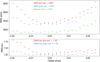 |
Fig. A.1 Top: RMS before (red circles) and after (blue circles) wiggle correction for the visit on 2022 July 03. Bottom: after performing the wiggle correction, the data show better agreement with the photon noise level. |
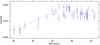 |
Fig. A.2 Spectral line detrending model for the 2021 March 24 dataset. A clear trend is visible between the stellar line contrast and the S/N at 550 nm. To characterize this relationship, we fit the out-of-transit data (filled disks) with a second-order polynomial (solid grey line). Using this best-fit model we perform a "vertical stretching" to the time series spectra to detrend the data accordingly. |
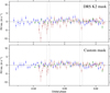 |
Fig. A.3 Time-series Keplerian RV residuals derived from DRS K2 (top) and custom (bottom) mask. Colours indicate different visits, where blue corresponds to 2021 March 24, green to 2022 July 03, and red to 2024 May 02. |
Appendix B AIT photometry
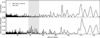 |
Fig. B.1 GLS periodogram of the AIT photometry (top) and the corresponding window function (bottom). The shaded region marks the Prot interval predicted from the activity-rotation relations of Suárez Mascareño et al. (2016), and the dash-dotted horizontal line in the top panel indicates the 10% false alarm probability level. |
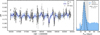 |
Fig. B.2 Gaussian process regression of the AIT photometry using a quasi-periodic kernel. Left: AIT light curve (black points) together with the median GP posterior model (blue line) and its 1σ credibility interval (shaded blue). Right: Posterior distribution of the stellar rotation period obtained from the GP kernel’s periodic hyperparameter. The dashed line shows a Gaussian fit to the mode of the distribution, and the grey shaded region marks the Prot interval predicted by the relations of Suárez Mascareño et al. (2016). |
Appendix C NGTS transit
Priors used and results obtained for the main planetary parameters from the NGTS transit fit.
Coefficients for the NGTS detrending models of the different cameras used during the NGTS transit fit.
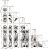 |
Fig. C.1 Posteriors of the transit fit to the NGTS data. |
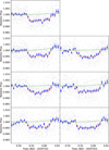 |
Fig. C.2 Individual light curves from the seven NGTS cameras. The best-fitting one-planet transit model, derived from a joint analysis of all the light curves, is shown as a solid yellow line. Baseline models for each camera are shown as dashed green lines. Grey dots indicate the unbinned data used in the fit, while blue squares show the data binned in 5-minute intervals for presentation purposes. |
Appendix D RMR analysis
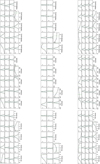 |
Fig. D.1 Posterior probability distributions of RVs (bottom row), contrast (middle row), and FWHM (top row) for three visits. The first, second, and third columns represent the observations from 2021 Mar 24, 2022 Jul 03, and 2024 May 02, respectively. The median value (solid blue line), the 1σ HDIs (dashed green lines), and the in-transit exposure index (shown at the upper-left corner) are displayed in each subpanel. |
Results for the individual fits to intrinsic time series properties, where the CCF profiles used for fitting are extracted using a CCF mask generated from the combined master spectrum of all three visits.
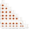 |
Fig. D.2 Correlation plots showing the PDFs and parameter dependencies in the global RMR analysis for model G1. The 1D histograms show the projected posterior distributions for each parameter, with dashed yellow lines marking the 68.3% HDIs and blue lines indicating the median values. The two black 2D contours correspond to the 1σ and 2σ confidence regions, containing 39.3% and 86.5% of the accepted MCMC steps, respectively. |
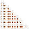 |
Fig. D.3 Correlation plots for model G2. For a detailed description, refer to the caption of Fig. D.2. |
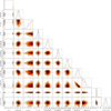 |
Fig. D.4 Same as Fig. D.3 but adopting a tighter prior on the stellar rotation period, Prot ∼ U(1, 40) days. |
Appendix E Classical RM analysis
We use the Python-based ARoME routine12 (Boué et al. 2013) to analyze the radial velocities of HAT-P-26 b (three transits: 2021 March 24, 2022 July 03, and 2024 May 02). The velocities were previously flattened by removing the Keplerian signal of the planet and the systemic velocity following the steps described in the main text. The observing times are folded in phase using the planetary ephemeris of Table A.1. The ARoME routine was conceived to model planetary RM effects using observations done by the Gaussian fit of CCFs. In our analysis, we fix the stellar limb darkening coefficients to the values of Table A.1 and the width of the instrumental profile to 2 km s−1, and set normal priors on the planet-to-star radius, orbital semimajor axis (in units of the star’s radius), and orbital inclination angle. The projected planetary obliquity, λ, and the stellar rotation, νeq sin i∗, are free with uniform priors in the intervals [−180, 10] deg and [0, 10] km s−1, respectively. We then apply a MCMC process for finding the best fit and constraining the uncertainties associated with the free variables. We used emcee (Foreman-Mackey et al. 2013) to perform MCMC simulations with 11 walkers, 5,000 iterations for burn-in, and another 5,000 for sampling the posteriors.
The MCMC analysis yielded the following results: λ =  deg and νeq sin i⋆ = 0.90 ± 0.12 km s−1. The posterior distributions are shown in Fig. E.1, and the best-fit model together with the observed data are displayed in Fig. E.2. The amplitude of the RM effect is approximately 0.66 m s−1, placing it among the smallest amplitudes reported in the literature. This is consistent with the star’s low projected rotational velocity. As with the RMR method, the projected planetary obliquity obtained from the classical RM analysis indicates a strong misalignment with respect to the stellar spin axis. However, the value derived here is somewhat more negative than those reported in Table 1, although still consistent at the 1 σ level. The main discrepancy between the classical analysis and the RMR method arises in the inferred νeq sin i∗ values: while RMS yields ∼0.23 km s−1, the classical approach returns a value nearly four times larger. Nonetheless, the two measurements remain compatible at the 3-4 σ level, and in the classical analysis νeq sin i∗ is detected at the 7.5σ confidence level.
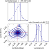 |
Fig. E.1 Posteriors distributions of the classical analysis of the RM effect. |
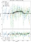 |
Fig. E.2 Top: Flattened radial velocities of HAT-P-26 b (colored dots) as a function of planetary orbital phase, together with the best-fit model obtained with ARoME (solid black line). The black squares represent the median radial velocities, while the grey-shaded area corresponds to the 1 σ uncertainty of the model. The vertical dashed lines indicate the planetary ingress and egress phases. Bottom: Observed minus computed data. |
Appendix F Considering whether the two planets are in a mean-motion resonance
HAT-P-26 b has been shown to have transit timing variations (TTVs), hinting at the presence of a third body in the system. The spectroscopic analysis of the discovery article showed a drift in the radial velocities with a significance detection of 2.1σ (Hartman et al. 2011). Stevenson et al. (2016) found a weak curvature in the transit timing residuals of six epochs spanning over 500 cycles (over 2000 days). Since then, several other works have performed detailed TTV analyses, increasing the number of transits analyzed and the time baseline. von Essen et al. (2019) found sinusoidal TTVs with semi-amplitude of 2.1 min and a period of 270 epochs. Mancini et al. (2022) found a similar behavior, with TTVs following a sinusoid with semi-amplitude of 1.6 min and period of 27 epochs. Recently, A-thano et al. (2023), with an analysis of a total of 39 transits spanning over 7 years, also found sinusoidal TTVs with a semi-amplitude of about 2 min and a slightly shorter period of 222 epochs. These variations could be due to an additional planet in the system (with a mass of ∼0.02 MJ and orbital period of 8.47 d, i.e, in a 1:2 MMR). Weak hints of a secondary planet were reported by Dévora-Pajares et al. (2024) from a search for transiting planets in TESS data. However, this candidate has an orbital period of 6.59 d and inferred mass of about 5 M⊕, different than the TTV-inferred planet from A-thano et al. (2023).
Although MMR configurations have been widely reported (e.g., Fabrycky et al. 2014), such resonant configurations are generally fragile, particularly for eccentric orbits and in the presence of additional stellar-mass perturbations. Motivated by this inconsistency in HAT-P-26 system, we performed a detailed orbital inversion using TTVs reported in A-thano et al. (2023), employing an inversion technique based on TTVFast (Deck et al. 2014; see details in Sun et al. 2025). Our inversion did not reveal any preferred solution consistent with an MMR configuration (see Fig. F.1). Given that uniquely constraining the parameters of a single transiting planet from TTVs alone remains challenging even with improved data quality (e.g., Nesvorný et al. 2013), we did not attempt to derive a best-fit model.
 |
Fig. F.1 TTV inversion results. The three colors correspond to independent fitting runs used to assess the robustness of the solution. |
All Tables
Comparison of properties of CCFs generated with the custom mask and the DRS K2 mask.
Priors used and results obtained for the main planetary parameters from the NGTS transit fit.
Coefficients for the NGTS detrending models of the different cameras used during the NGTS transit fit.
Results for the individual fits to intrinsic time series properties, where the CCF profiles used for fitting are extracted using a CCF mask generated from the combined master spectrum of all three visits.
All Figures
|
Fig. 1 Distribution of orbital period versus radius for close-in exoplanets. The boundaries for the refined classification (Neptunian desert, ridge, and savanna; Castro-González et al. 2024a) are shown as dashed lines. Neptunes with well-measured 3D spin–orbit angles (precision better than 30° in the TEPCat catalog1) are marked with crosses. Squares represent planets with (red edge) or without (magenta edge) escaping H/He detections. HAT-P-26 b is marked with a star. The radius and mass values are taken from the NASA Exoplanet Archive2. |
| In the text | |
|
Fig. 2 Observational logs of the four ESPRESSO visits, including airmass, seeing, and S/N around 550 nm (orders 102 and 103). For each visit, the median exposure time and the mean value of the integrated water vapor (IWV) content are shown in the legend. Grey-shaded regions indicate the out-of-transit phases, highlighting the transit window. |
| In the text | |
|
Fig. 3 NGTS transit data taken on 2022 July 03. Black data points show the average of all seven cameras used binned to 5 minutes and airmass-detrended, and orange line shows the best fit model. |
| In the text | |
|
Fig. 4 Properties (dots) of the stellar surface occulted by the planet, along with the best-fit RMR model (M1, black lines) from the global fit. The measured properties from three visits are color-coded as in Fig. 2: blue for 2021 March 24, green for 2022 July 03, and yellow for 2024 May 02. The error bars represent the 1σ highest density intervals (HDIs), which correspond to the dashed green lines in Fig. D.1. To improve the visualization of the global fit, data points from all three visits are binned to a phase resolution of 0.0015 (black diamonds). The transit contacts are marked by the vertical dotted grey lines. |
| In the text | |
|
Fig. 5 2D maps of the intrinsic CCF profiles (top), their RMR model estimates (middle), and the residuals (bottom) for the three visits on 2021 March 24 (first column), 2022 July 03 (second column), and 2024 May 02 (third column). Dashed green lines mark the four transit contacts. Solid green line in the residual maps shows the best-fit global, model G1. |
| In the text | |
|
Fig. 6 Posterior distribution of the 3D spin–orbit angle ψ, derived by assuming a uniform prior on cos i⋆ (random stellar spin axis orientation). The purple and blue density contours represent the posterior distributions of ψ under the projected obliquity constraints from the RMR analysis and the classical RM analysis respectively, while the solid curves mark the 1, 2, and 3σ credible regions. The red point indicates the ψ value obtained from the RMR G2 fit. The side panel shows the 1D marginal posteriors of ψ. Both distributions consistently favor a polar orbital configuration. |
| In the text | |
|
Fig. 7 Precession frequencies of vPla/Star (red), vStar/Pla (orange), vComp/Pla (cyan), and v>Pla/Comp (blue) as a function of the stellar rotation period. The background shading denotes different dynamical regimes: dynamically coupled (white), Hybrid (i) (green), Cassini (a) (yellow), and Pure orbit (b) (blue). The predicted 3D spin–orbit angles for regimes (i), (a), and (b) are given in Boué & Fabrycky (2014). |
| In the text | |
|
Fig. 8 Density distribution versus orbital period (top) and EMF versus planetary mass (bottom) for close-in Neptunes. In the top panel, all close-in Neptunes (3.5 R⊕ < Rp < 8.5R⊕, P < 30 days) are shown as grey dots with symbol size scaled to planetary radius. A subset with available 3D spin–orbit measurements is highlighted using distinct face colors, and planets on polar orbits (72°-108°) are emphasized in yellow. The Neptunian sample with EMF estimates from Doyle et al. (2025) is indicated by the blue and red boxes, as illustrated in the bottom panel. A dotted line marks the bulk-density level of 1 g cm−3, and the approximate brink boundary proposed by Bourrier et al. (2025) is shown as a dashed line. The ridge corresponds to the green-shaded region. In the bottom panel, the warmer Neptunes (Teff> 1300 K; red squares) have EMF values close to zero, indicating almost no surviving envelopes. While, the cooler sample (Teff ≤ 1300 K; gradient blue squares), as proposed by Doyle et al. (2025), follows the linear trend (solid blue line). Samples with only EMF upper limits are marked by triangles, and ridge planets are highlighted with light green outlines. |
| In the text | |
|
Fig. 9 Results from the N-body ZLK migration simulations of HAT-P-26 b. Left to right : semimajor axis, ab, stellar obliquity, ψAb, mutual inclination, ψbB, between the orbits of planet b and companion B, and the orbital eccentricity, eb. Dashed and dotted black lines mark the observed values and 1σ uncertainties. |
| In the text | |
|
Fig. A.1 Top: RMS before (red circles) and after (blue circles) wiggle correction for the visit on 2022 July 03. Bottom: after performing the wiggle correction, the data show better agreement with the photon noise level. |
| In the text | |
|
Fig. A.2 Spectral line detrending model for the 2021 March 24 dataset. A clear trend is visible between the stellar line contrast and the S/N at 550 nm. To characterize this relationship, we fit the out-of-transit data (filled disks) with a second-order polynomial (solid grey line). Using this best-fit model we perform a "vertical stretching" to the time series spectra to detrend the data accordingly. |
| In the text | |
|
Fig. A.3 Time-series Keplerian RV residuals derived from DRS K2 (top) and custom (bottom) mask. Colours indicate different visits, where blue corresponds to 2021 March 24, green to 2022 July 03, and red to 2024 May 02. |
| In the text | |
|
Fig. B.1 GLS periodogram of the AIT photometry (top) and the corresponding window function (bottom). The shaded region marks the Prot interval predicted from the activity-rotation relations of Suárez Mascareño et al. (2016), and the dash-dotted horizontal line in the top panel indicates the 10% false alarm probability level. |
| In the text | |
|
Fig. B.2 Gaussian process regression of the AIT photometry using a quasi-periodic kernel. Left: AIT light curve (black points) together with the median GP posterior model (blue line) and its 1σ credibility interval (shaded blue). Right: Posterior distribution of the stellar rotation period obtained from the GP kernel’s periodic hyperparameter. The dashed line shows a Gaussian fit to the mode of the distribution, and the grey shaded region marks the Prot interval predicted by the relations of Suárez Mascareño et al. (2016). |
| In the text | |
|
Fig. C.1 Posteriors of the transit fit to the NGTS data. |
| In the text | |
|
Fig. C.2 Individual light curves from the seven NGTS cameras. The best-fitting one-planet transit model, derived from a joint analysis of all the light curves, is shown as a solid yellow line. Baseline models for each camera are shown as dashed green lines. Grey dots indicate the unbinned data used in the fit, while blue squares show the data binned in 5-minute intervals for presentation purposes. |
| In the text | |
|
Fig. D.1 Posterior probability distributions of RVs (bottom row), contrast (middle row), and FWHM (top row) for three visits. The first, second, and third columns represent the observations from 2021 Mar 24, 2022 Jul 03, and 2024 May 02, respectively. The median value (solid blue line), the 1σ HDIs (dashed green lines), and the in-transit exposure index (shown at the upper-left corner) are displayed in each subpanel. |
| In the text | |
|
Fig. D.2 Correlation plots showing the PDFs and parameter dependencies in the global RMR analysis for model G1. The 1D histograms show the projected posterior distributions for each parameter, with dashed yellow lines marking the 68.3% HDIs and blue lines indicating the median values. The two black 2D contours correspond to the 1σ and 2σ confidence regions, containing 39.3% and 86.5% of the accepted MCMC steps, respectively. |
| In the text | |
|
Fig. D.3 Correlation plots for model G2. For a detailed description, refer to the caption of Fig. D.2. |
| In the text | |
|
Fig. D.4 Same as Fig. D.3 but adopting a tighter prior on the stellar rotation period, Prot ∼ U(1, 40) days. |
| In the text | |
|
Fig. E.1 Posteriors distributions of the classical analysis of the RM effect. |
| In the text | |
|
Fig. E.2 Top: Flattened radial velocities of HAT-P-26 b (colored dots) as a function of planetary orbital phase, together with the best-fit model obtained with ARoME (solid black line). The black squares represent the median radial velocities, while the grey-shaded area corresponds to the 1 σ uncertainty of the model. The vertical dashed lines indicate the planetary ingress and egress phases. Bottom: Observed minus computed data. |
| In the text | |
|
Fig. F.1 TTV inversion results. The three colors correspond to independent fitting runs used to assess the robustness of the solution. |
| In the text | |
Current usage metrics show cumulative count of Article Views (full-text article views including HTML views, PDF and ePub downloads, according to the available data) and Abstracts Views on Vision4Press platform.
Data correspond to usage on the plateform after 2015. The current usage metrics is available 48-96 hours after online publication and is updated daily on week days.
Initial download of the metrics may take a while.