


| Issue |
A&A
Volume 711, July 2026
|
|
|---|---|---|
| Article Number | A200 | |
| Number of page(s) | 17 | |
| Section | Interstellar and circumstellar matter | |
| DOI | https://doi.org/10.1051/0004-6361/202558550 | |
| Published online | 14 July 2026 | |
The multiphase interstellar medium as a common origin for magnetic misalignment and TB parity violation
1
LUX, Observatoire de Paris, Université PSL, Sorbonne Université, CNRS,
75014
Paris,
France
2
INAF – Osservatorio Astrofisico di Arcetri,
Largo E. Fermi 5,
50125
Firenze,
Italy
3
Laboratoire de Physique de l'Ecole Normale Supérieure, ENS, Université PSL, CNRS, Sorbonne Université, Université de Paris,
75005
Paris,
France
4
Department of Physics, California Institute of Technology,
Pasadena,
CA
91125,
USA
5
TAPIR, California Institute of Technology,
MC 350-17,
Pasadena,
CA
91125,
USA
★ Corresponding author: This email address is being protected from spambots. You need JavaScript enabled to view it.
Received:
12
December
2025
Accepted:
21
May
2026
Abstract
We present an original data analysis and a physical model that provide new insights into the origin of and relationship between two observables of the dusty polarized Galaxy at intermediate and high latitudes: (i) the misalignment between HI filamentary structures and magnetic fields and (ii) the positive T B correlation measured in Planck data suggesting parity violation in the interstellar medium (ISM). We confirm an observational link between the two effects and find that both are predominantly produced at large angular scales (≥10°, multipoles ℓ ≤ 20), with a significantly stronger signal in the northern hemisphere. We propose a model in which filaments and magnetic fields appear misaligned in projection because they are sourced by cold and warm gas phases distributed in different proportions in the solar neighborhood, from the wall of the Local Bubble to larger distances. These projection effects at large angular scales can produce coherent signatures that propagate to smaller scales in power spectra without invoking local, small-scale filament misalignment. Within this frame, H I filaments remain statistically aligned with the magnetic field in 3D, although with a projected scatter of tens of degrees that requires further investigation. The multiphase, geometrical model presented in this work is supported by Planck polarization data at 30 GHz, where synchrotron radiation dominates, and at 217 and 353 GHz, where dust emission dominates. Our analysis also incorporates starlight polarization measurements. The model introduced here suggests a new interpretation of two unexplained observables and emphasizes the role of the large-scale magnetized ISM in shaping polarized Galactic emission, which has important implications for both Galactic astrophysics and cosmological foreground characterization.
Key words: dust, extinction / ISM: magnetic fields / ISM: structure / local insterstellar matter / solar neighborhood / cosmic background radiation
Hubble Fellow.
© The Authors 2026
 Open Access article, published by EDP Sciences, under the terms of the Creative Commons Attribution License (https://creativecommons.org/licenses/by/4.0), which permits unrestricted use, distribution, and reproduction in any medium, provided the original work is properly cited.
This article is published in open access under the Subscribe to Open model. This email address is being protected from spambots. You need JavaScript enabled to view it. to support open access publication.
1 Introduction
The filamentary interstellar medium (ISM) has recently emerged as a key research focus in the study of dusty and gaseous density structures that feed stellar nurseries in the Galaxy (e.g., André et al. 2010; Hacar et al. 2023; Pineda et al. 2023). It also plays an important role in the characterization of Galactic foregrounds affecting cosmological signals in the context of cosmic microwave background (CMB) polarization experiments (e.g., Clark et al. 2015; Planck Collaboration Int. XXXVIII 2016; Planck Collaboration XI 2020; Clark et al. 2021; Cukierman et al. 2023; Halal et al. 2024; Hervías-Caimapo et al. 2025).
Polarized dust emission, which is produced by paramagnetic grains aligning with magnetic fields (e.g., Hoang et al. 2018, references therein), is a dominant foreground component for cosmological studies of the submillimeter sky. Dust emission obstructs accurate measurements of CMB polarization statistics, which are usually expressed in terms of angular power spectra (BICEP2/Keck & Planck Collaborations 2015; Planck Collaboration Int. XXX 2016). These spectra are the standard tools for quantifying the cosmological, scale-dependent amplitudes of temperature (total intensity) anisotropies (T) as well as parity-even (E) and parity-odd (B) modes of polarized anisotropies generated at the last-scattering surface in the early Universe (e.g., Zaldarriaga 2001).
While parity symmetry holds in the standard cosmological model, leading to vanishing T B and E B correlations (Zaldarriaga & Seljak 1997), nonstandard theories suggest the possibility of parity violation, either during inflation (e.g., Lue et al. 1999) or through the interaction of CMB photons with parity-violating pseudo-scalar fields (e.g., axions) during cosmic expansion (e.g., Komatsu 2022). These violations could leave observable signatures, such as cosmic birefringence, producing nonzero T B and E B cross-spectra. These cosmological signatures remain undetected, with current studies providing only upper limits (e.g., Planck Collaboration Int. XLIX 2016; Eskilt & Komatsu 2022). In addition to the technological challenge of achieving the sensitivity and systematic control required for precision polarization measurements (e.g., Ritacco et al. 2024), potential sources of T B correlation may also arise from Galactic polarized foregrounds. A nonzero T B signal has been measured in the Milky Way by the Planck satellite at 353 GHz (Planck Collaboration XI 2020). This signal is primarily detected at large angular scales, corresponding to multipoles of ℓ ≤ 500, and it has also been confirmed at 23 GHz in data from the Wilkinson Microwave Anisotropy Probe (WMAP, Weiland et al. 2020). Despite these detections, a clear physical explanation for the Galactic T B correlation remains elusive.
Two main hypotheses have been proposed. (1) The nonzero T B correlation may arise from a misalignment of filamentary density structures and their local magnetic field (e.g., Huffenberger et al. 2020; Clark et al. 2021; Hervías-Caimapo & Huffenberger 2022; Cukierman et al. 2023; Hervías-Caimapo et al. 2025). (2) As proposed by Bracco et al. (2019a) and further explored by Weiland et al. (2020), the T B correlation may be imprinted by the large-scale structure of the magnetized ISM in the solar neighborhood without relying on the local small-scale magnetic misalignment.
The misalignment hypothesis is supported by observational evidence linking, in projection, filamentary density structures to the morphology of the magnetic field in the ISM. Based on dust polarization data, interstellar magnetic fields have been found to be statistically aligned with density structures in the diffuse ISM (with column densities ≤1022 cm–2), becoming progressively perpendicular in denser molecular-cloud regions (Planck Collaboration Int. XXXII 2016; Planck Collaboration Int. XXXV 2016). The relative orientation between filamentary structures and magnetic fields naturally induces cross-correlations among T, E, and B modes. As predicted by Zaldarriaga (2001) and measured in several analyses of Planck data, the observed variation in relative orientation produces a positive T E correlation in the diffuse ISM (Planck Collaboration Int. XXXVIII 2016) and a vanishing T E in molecular clouds (Bracco et al. 2019b). In this framework, the T B correlation could result from a statistical oblique misalignment between filamentary density structures and the local magnetic-field orientation. A misalignment angle on the order of a few degrees has been measured by comparing the morphology of the diffuse density structure, traced by atomic hydrogen (H I), with the magnetic field, traced by Planck polarization (Clark et al. 2015, 2021; Cukierman et al. 2023; Halal et al. 2024). These results support the hypothesis that magnetically misaligned filamentary structures could contribute to the nonzero T B correlation measured by Planck. However, the mechanisms inducing this misalignment remain unknown. The coherent oblique misalignment on the sky is surprising given that turbulence dynamics relax to configurations where density structures align parallel or perpendicular to the magnetic field (Soler & Hennebelle 2017).
The large-scale-structure hypothesis addresses the issue of coherence by invoking the specific viewpoint of the solar neighborhood within the larger Galaxy. We note that in Bracco et al. (2019a), the T B correlation was modeled only for multipoles ℓ < 25, whereas Planck results show a nonzero T B signal even at higher multipoles. This apparent contradiction could be resolved by recognizing that dust polarization observations do not continuously sample the large-scale magnetic field structure. Due to the sparse ISM density distribution, even a low-multipole (large-scale) feature in the magnetic-field structure could be modulated to higher multipoles (smaller scales). However, this large-scale picture has yet to provide a physical explanation for the origin of the misalignment.
In this work, we present a novel analysis of both the misalignment angle and the T B correlation, and we introduce a physical scenario that builds on the two aforementioned hypotheses. Our interpretation is based on purely geometrical arguments in the context of the multiphase, magnetized ISM in the solar neighborhood. In the following, we introduce our assumptions and briefly describe the physical scenario.
The polarized sky at high Galactic latitudes is determined by the combination of the magnetic field of the Local Bubble (LB), a hundreds-of-parsec cavity around the Sun carved by several supernovae (Pelgrims et al. 2020; Zucker et al. 2022), and the Galactic mean field at larger scales.
We assumed the gas at high latitudes is a two-phase medium composed of a mass-weighted cold (CNM) and volume-filling warm (WNM) neutral media (Wolfire et al. 2003). Dust polarization traces both components, while the H I-filamentary structures, obtained through local spatial filtering of spectroscopic data, only trace the CNM (see also, Clark et al. 2019).
The CNM filaments are considered compressed structures on the surface of the LB (e.g., Inoue & Inutsuka 2016), contributing to the majority of the T morphology of dust intensity, and are statistically aligned with the LB magnetic field.
The observed misalignment angle, measured as a large-scale effect (ℓ < 20), is the result of projection effects along the line of sight between the LB field, traced by the CNM, and its superposition with the mean field in the spatially larger WNM. A different morphology of the LB field with respect to the mean field (e.g., Alves et al. 2018) can imprint large-scale polarization structures, sourcing both the sign of the misalignment and the T B correlation.
We support this scenario using multiwavelength, high-Galactic-latitude observations in polarization including H I data; Planck data at 30, 217, and 353 GHz; and starlight polarization measurements. The paper is organized as follows. In Sect. 2, we describe the multiple datasets used in the analysis. In Sect. 3, we detail the measurement of the misalignment angle. In Sect. 4, we present the main observational results of the paper, namely the dependence of the misalignment angle on sky fraction, angular scale, and polarization fraction. In Sect. 5, we discuss the results and introduce the geometrical interpretation of the misalignment angle and the T B correlation. We conclude in Sect. 6 and include five appendices.
2 Data
In this section, we describe the various datasets used in the analysis. Both H I and Planck data are presented.
2.1 Planck data
We employed Planck polarization data at three different frequencies: 30, 217, and 353 GHz. The higher frequencies are dominated by thermal emission from dust, while the 30-GHz data trace non-thermal synchrotron radiation. In the case of dust frequencies, we considered two sets of Stokes Q and U maps (hereafter, Qk,d and Uk,d, where the subscript "k" represents the frequency index and the subscript "d" indicates dust) produced by different processing methods, which both improved systematic effects in polarization of Planck data compared to the legacy products of the public release (PR) 3 (Planck Collaboration I 2020).
First, we used the SRoll2 maps (Delouis et al. 2019). The dominant systematic effect for the polarized signal at 353 GHz in the PR 3 maps is related to the measurement of the time transfer function of the detectors; at lower frequencies, it is the non-linearity of the analog-to-digital converters. Both systematics have been improved in a consistent way with all other known effects for the SRoll2 dataset. Second, we used the PR4 maps produced with the NPIPE processing pipeline (Planck Collaboration Int. LVII 2020), whose main improvements over PR3 are lower noise and systematics as well as greater internal consistency among the frequency channels.
At 353 GHz, we used the Stokes I map produced with the Generalized Needlet Internal Linear Combination (GNILC) method (hereafter, Id), which is corrected for fluctuations of the CMB and the cosmic infrared background (CIB). However, the value of the CIB monopole that must be subtracted is 0.13 MJy sr−1 as reported in Planck Collaboration XII (2020); this is crucial to correctly estimate the dust polarization fraction, especially at high latitudes, where the Galactic emission becomes dimmer. We denote polarization fraction by
 (1)
(1)
where Pd is referred to as the polarized intensity. In order to convert units from KCMB to MJy sr−1 at 353 GHz, we used the conversion factor 287.5 (Planck Collaboration XII 2020). In the case of the Stokes parameters at 30 GHz (hereafter, Qs and Us, where the subscript "s" indicates synchrotron radiation), we considered two distinct datasets from PR3 and PR4, respectively. In the following, all maps are in HEALPix1 format (Górski et al. 2005). The data of reference are Q353,d and U353,d because dust polarized emission is maximum there. In order to neglect noise bias in polarization over the full sky at 353 GHz, the best angular resolution of all maps is a full-width half-maximum (FWHM) of 80' (Planck Collaboration XII 2020). For this FWHM, the corresponding pixel resolution is determined by the HEALPix parameter Nside = 128 (~30' pixel width). All maps are smoothed and projected on the same sky grid using the healpy Python package (Zonca et al. 2019).
2.2 HI data
We used two polarization templates derived from maps of H I emission2. Each technique identifies the orientations of filamentary H I structures and infers a plane-of-sky magnetic-field orientation, which implies a perpendicular dust polarization angle. The two techniques are described in Sect. 3 of Halal et al. (2024), and the H I maps are drawn from the spectro-scopic data cubes of HI4PI Collaboration (2016) with velocities between −13 and 16 km s−1. One template is formed from the Hessian matrix of the H I brightness temperature; the polarization angle is based on locations of negative curvature, and the associated polarization intensity is based on the Hessian eigenvalues. The second template is based on the spherical rolling Hough transform (SRHT), which weights linear structures according to their local orientations; this allows for a superposition of orientations, and the polarization intensity is based on the H I brightness temperature. When comparing the two H I maps (hereafter, "H I templates") with the Planck polarization data, we smoothed them to the same FWHM and pixel resolution.
2.3 Starlight polarization catalog
In Sect. 5.2.3, we study the dependence of polarization-angle differences on heliocentric distance. For this analysis, we use the most recently compiled starlight polarization catalog with distance estimates from Gaia (Panopoulou et al. 2025). Starlight polarization provides complementary information to the dust thermal emission, as it is the result of extinction on dust grains along the line of sight and allows one to trace the magnetic field orientation averaged from the observer to the stars (Hiltner 1949; Davis & Greenstein 1951; Hildebrand 1988). We stress that, while dust polarization in emission traces the orthogonal orientation to the magnetic-field on the plane of the sky, starlight polarization directly traces the magnetic-field orientation.
We considered stars with a polarization angle uncertainty smaller than 5° (or a signal-to-noise in degree of polarization on the order of 5). We projected the star catalog onto HEALPix grids with Nside = 128, averaging over any multiple starlight measurements within the same HEALPix pixel (see Sect. 5.2.3). We verified that our results are robust to changes in the pixelation.
3 Methods
We computed the relative orientation between two sets of polarization angles i and j, namely, ψi = 0.5 × atan2(Ui, Qi) and ψj = 0.5 × atan2(Uj, Qj), as follows,
 (2)
(2)
where 𝒜ij = (sin 2ψi cos2ψj − cos 2ψi sin 2ψi) and ℬij = (cos 2ψi cos 2ψj + sin 2ψi sin 2ψj) (see also, Planck Collaboration Int. XXXII 2016; Clark et al. 2015). We note that, in this work, the sign of the polarization angles is positive for consistency with the IAU convention and the notation used in Cukierman et al. (2023); following the HEALPix convention, however, a minus sign would appear in Eq. 2 (e.g., Planck Collaboration Int. XLIV 2016).
In Sect. 5.3.1, as part of the link between T B correlation and misalignment angle, we form smoothed versions of the polarization maps in order to estimate the polarization angles associated with large-scale features. We use the large-scale polarization angles to de-rotate the original, unsmoothed maps. This has the effect of removing the prevailing orientations of large-scale polarization features. The smoothed map is determined by a given FWHM represented by the multipole ℓref, i.e., FWHM = 180°/ℓref. The rotated Stokes parameters (labeled with the superscript "R") were obtained using the following rotational transform:
 (3)
(3)
where x denotes an index that can be either i or j. As an example, in Fig. A.1 the case for ℓref = 20 is shown applied to Q353,d and U353,d.
In Sect. 4.1, we study how the histograms of Δψ, normalized probability distribution functions (NPDFs), vary across the sky. In particular, we made use of four distinct masks delivered by the Planck Collaboration3, which cover progressively larger portions of the sky, ranging from 20 to 80% with steps of 20%. These masks are produced by masking out incrementally brighter thermal dust emission. Figure 1 displays these masks in different colors on a galactic coordinate grid. The masks approximately correspond to selections of sky areas by Galactic latitude, such that the 20% mask mostly includes regions at |b| > 60°. Averaging the NPDFs obtained by using Eq. (2) among all distinct data versions (i.e., SRoll2, PR4, SRHT, Hessian), in the following we show their mean distribution, Δψ, and the corresponding standard deviation. The impact of residual systematic effects in the Planck data on the NPDFs is quantified by calculating the angle difference between the SRoll2 and PR4 datasets and is shown as a gray shaded area in the figures.
In Sect. 4.2, focusing on the 20% mask, we explore how the NPDFs of Δψ depend on angular scale in the two Galactic hemispheres. We computed Δψ after smoothing both the Planck data and the H I templates to progressively lower angular resolutions, parameterized by the multipole ℓFWHM = 180/FWHM [deg]. To avoid leakage from bright emission at low Galactic latitudes, we applied the 40% mask to the Stokes parameters before smoothing. We further applied a positive (negative) Galactic latitude criterion to the 40% mask to isolate the northern (southern) hemisphere. The masks were also smoothed with a Gaussian beam to minimize artifacts introduced by the smoothing process.
Throughout the analysis, we maintained a fixed pixelization, independent of the smoothing kernel. While this resulted in over-sampling of the beam at low angular resolution, it allowed us to retain the same number of sky pixels in the Δψ NPDFs. We verified that the results remained robust when re-pixelizing the maps to lower values of Nside, ensuring they remained within the Nyquist-sampling limit. In Sect. 5.3.1, in order to explore the impact of large-scale features on the dust polarization power spectra at small scales, we use the Planck and H I-template maps at FWHM=15' with Nside = 512.
 |
Fig. 1 All-sky masks with sky fractions of 20, 40, 60, and 80% with progressively brighter colors. The gray region along the Galactic plane is not considered in this work. A galactic coordinate grid with steps of 30° in longitude l and latitude b is overlaid with its origin at the Galactic center. |
4 Results
In this section, we report the observational results on the angle difference Δψ between Planck polarization data at 353 GHz and the H I templates. We present the dependence of Δψ on sky fraction, on pd and on angular scale.
4.1 Misalignment as a function of sky fraction and pd
By applying Eq. (2), we computed Δψ and corresponding NPDFs for combined and separate Galactic hemispheres using data at FWHM=80'. In Fig. 2, we show the NPDFs of Δψ, their circular means4 〈Δψ〉circ and their spread σ(Δψ) as a function of sky fraction. The central panels include gray shadows representing Δψcirc values computed using the difference between SRoll2 and PR4 polarization data, a measure of residual systematic effects in the Planck data. In the top panels, errors on the NPDFs reflect variance across different versions of the same dataset used for each tracer, namely, dust polarization and H I templates.
Firstly, we observe that all NPDFs exhibit a large value of σ(Δψ), which is approximately 30° in both Galactic hemispheres. The only significant variation of σ(Δψ), of about a factor of three, is found with respect to pd. In Fig. 3, we show the NPDFs of Δψ as a function of nine equally sampled bins of pd. Each bin contains 15633 sky pixels. We verified that results are robust to changes in the number of bins. The central value of each pd bin is plotted on the x axis in the central and bottom panels of the figure. The corresponding NPDFs are shown in the top panel with brighter (darker) colors for lower (larger) values of pd. As shown by the bottom panel, σ(Δψ) varies from 40° to 15°, spanning from low to large values of pd in the 80% mask. This result shows that σ(Δψ) is the lowest when pd is the largest. As pd is maximum when the magnetic field is perpendicular to the line of sight (e.g., Planck Collaboration Int. XLIV 2016), the trend of σ(Δψ) that we observed is most likely determined by projection effects, i.e., H I templates more closely align with dust polarization when the magnetic field is perpendicular to the line of sight (see also, Clark & Hensley 2019). We notice, however, that at FWHM=80' even for the largest pd values, σ(Δψ) is yet larger than 10°, highlighting a significant dispersion around the alignment.
Secondly, we observe that although the NPDFs generally peak at 〈Δψ〉circ ≈ 0°, this is not the case for the 20% mask at high Galactic latitudes, where a misalignment of 4.5° ± 0.9°5 occurs on average across the two hemispheres, in agreement with previous findings (e.g., Clark et al. 2021; Cukierman et al. 2023). This misalignment is more prominent in the northern hemisphere, reaching a value of 〈Δψ〉circ = 6.5° ± 0.6°, significantly exceeding the contributions from systematic effects. In the southern hemisphere the misalignment is always consistent with systematic effects. In the northern Galactic hemisphere, we notice that the misalignment remains significant in the 40% mask at lower Galactic latitudes. In the central panel of Fig. 3, we also observe that the misalignment is independent of pd for values larger than 0.03. The level of misalignment in the 80% mask is about 2° and drops to 0° for pd < 0.03, where data noise is likely contributing to the NPDFs. We stress that the value of ~2° is not comparable with what is shown in Fig. 2, where we computed the misalignment angle averaged in the 20% of the sky between the 80 and the 60% masks.
4.2 Misalignment as a function of scale
Using the 20% mask, we explored the dependence of Δψ on angular scale in two separate but complementary ways. First, we computed Δψ after smoothing the Planck data and the H I templates to progressively lower values of ℓFWHM. In Fig. 4, we show the NPDFs of Δψ as a function of ℓFWHM. We observe an increase in misalignment at large angular scales, while σ(Δψ) remains uniform, suggesting that data noise is not the dominant contribution to σ(Δψ). These effects occur in both Galactic hemispheres with the same misalignment sign. The largest misalignment, approximately 12° ± 3°, occurs at ℓFWHM = 4.5. At these scales, the misalignment becomes significant compared to systematic effects, even in the southern Galactic hemisphere. We also notice that at larger multipoles (ℓ > 10) the two hemispheres behave differently, with a rather flat and coherent misalignment in the north and a decreasing misalignment in the south, which is consistent with systematic effects for all smoothing scales.
Second, we computed Δψ from high-pass-filtered Stokes parameters and H I templates, retaining only power up to angular scales corresponding to multipoles ℓmin = 180°/max_scale. Using a Gaussian filter, we removed power at multipoles less than ℓmin. This analysis, shown in Fig. 5 with the respective NPDFs, confirms that the observed misalignment between Planck data and H I templates is predominantly a large-scale phenomenon, manifesting only at the largest scales including the dipole.
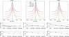 |
Fig. 2 Normalized probability distribution functions of Δψ between Planck data at 353 GHz and the H I templates. The value of Δψ is computed for different sky masks at angular and pixel resolutions of 80' and Nside = 128, respectively. The NPDFs are shown for both Galactic hemispheres combined (central panels) and for the southern (left panels) and northern (right panels) hemispheres individually. The corresponding circular-mean values (in black circles) and their standard deviations (in gray diamonds) are shown in the insets at the bottom as a function of the sky mask. The gray shaded area in the middle panels represents the misalignment angle caused by systematic differences between SRoll2 and PR4 data. |
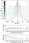 |
Fig. 3 The NPDFs of Δψ as a function of pd over the 80% mask. The NPDFs were computed in equally sampled bins of pd containing 15633 elements and are represented with bright to dark colors from low to large values of pd, respectively. The central value of each pd bin is plotted on the x axis in the central and bottom panels. The errors on 〈Δψ〉circ are smaller than the symbols. |
5 Discussion of large-scale misalignment
In this section, we discuss the large-scale misalignment and its implications for both understanding the magnetic-field structure in the solar neighborhood and interpreting the T B correlation in angular power spectra. The origin of misalignment between dust polarization and H I templates is investigated with two physical scenarios involving line-of-sight variations of either the dust emission or the magnetic-field structure probed by the multiphase H I gas. Our analysis supports the latter scenario.
5.1 First scenario: Variations in dust emission
The knowledge of the polarized spectral energy distribution (PSED) of interstellar dust is of primary importance both for characterizing the physical properties of dust grains in our galaxy (e.g., Guillet et al. 2018; Planck Collaboration XII 2020; Reissl et al. 2020) and for estimating foreground contamination to CMB polarization (e.g., Planck Collaboration XI 2020). However, it has been shown that a thorough understanding of the dust PSED may be strongly hampered by line-of-sight changes in dust properties (e.g., Tassis & Pavlidou 2015; Skalidis 2024; Mandarakas et al. 2025). As the observed dust polarization is determined by the emission-weighted Galactic magnetic field along the line of sight (e.g., Wardle & Konigl 1990; Lee & Draine 1985; Planck Collaboration Int. XX 2015), any changes in dust opacity and temperature could introduce effective frequency-dependent variations of polarization fraction and angle (e.g., Tram et al. 2024). This effect was measured in Planck data (e.g., Pelgrims et al. 2021; Ritacco et al. 2023). Since H I templates are sensitive to the magnetic-field orientation but not to dust properties, the observed misalignment with Planck data could be a signature of changes in dust emission (i.e., temperature and opacity) along the line of sight. Because the misalignment is predominantly at large scales, we may witness dust emissivity changes between the solar neighborhood within a few hundred parsecs and dusty regions on larger physical scales. As this scenario would imply frequency-dependent variations of the Planck polarization angle, we calculated Δψ using Planck data at 217 GHz. In Fig. B.1, we show the NPDFs of Δψ between H I templates and dust polarization at 217 GHz as a function of ℓFWHM. Comparing the NPDFs and the corresponding values of 〈Δψ〉circ with the 353-GHz results presented in Fig. 4, we obtain comparable misalignment at the two frequencies, which cannot be caused by known systematic effects in the Planck data. Although the values of 〈Δψ〉circ at 217 GHz are a few degrees lower than those at 353 GHz, they are consistent within the uncertainties. Given the level of precision, we are not able to detect significant variations of the misalignment between frequencies. This suggests that frequency decorrelation is unlikely measured by the NPDFs and that other mechanisms may be responsible for the misalignment between H I templates and dust polarization.
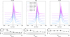 |
Fig. 4 The NPDFs of Δψ, considering the 20% mask and changing the angular resolution of the maps to ℓFWHM. Left and right panels show the southern and northern hemispheres, respectively. The central panel shows them together. More small-scale information is included as ℓFWHM increases. |
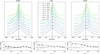 |
Fig. 5 Same as for Fig. 4 but filtering out the large angular scales up to ℓmin. Large-scale information is removed at ℓ < ℓmin as ℓmin increases. |
5.2 Second scenario: Changes in magnetic-field structure
The second scenario involves only geometric effects related to variations in the magnetic-field structure associated with different phases of the H I gas along the line of sight. Thermal dust emission is highly correlated with the H I brightness temperature at intermediate and high Galactic latitudes (e.g., Boulanger et al. 1996; Lenz et al. 2017). The H I gas exists as a bi-stable medium, comprising both the CNM (THI ≈ 100 K, NHI ≈ 50 cm−3) and the WNM (THI ≈ 8000 K, NHI ≈ 1 cm−3). These components, both containing interstellar dust, carry distinct temperatures and densities, with their relative proportions varying according to the Galactic environment (Wolfire et al. 2003; Ferrière 2020; Marchal & Miville-Deschênes 2021; Marchal et al. 2024).
Assuming that dust grains have uniform properties (such as temperature, opacity, and alignment with the magnetic field), we hypothesize that the H I templates and dust polarization are influenced by distinct orientations of the magnetic field, which varies with different mixtures of CNM and WNM along the line of sight. Specifically, at high Galactic latitude, the H I templates, derived from local spatial filtering of the H I brightness temperature at velocities between −13 and 16 km s−1 (Sect. 2.2), are thought to predominantly trace CNM filamentary structures on the LB surface (Clark et al. 2019). CNM also dominates the structure of dust total intensity. In contrast, dust polarization traces the line-of-sight superposition of both CNM and WNM. CNM density structures form through thermal instability, triggered by turbulence and shock-driven large-scale compressions, within the volume-filling WNM gas. These processes also impact the magnetic-field structure in both phases (e.g., Inutsuka et al. 2015; Inoue & Inutsuka 2016). The H I templates at high Galactic latitudes primarily map the magnetic field on the edges of the LB (Clark et al. 2019). Meanwhile, dust polarization provides combined information on the LB magnetic field and the regular magnetic field in the WNM over physical scales larger than the LB (>300 pc, O'Neill et al. 2024). For simplicity, in this work we have assumed a two-phase, two-layer model. This approximation may underestimate the presence of additional gas components along the line of sight, such as the unstable H I neutral medium (UNM), and their effects on the observed polarization. Multi-layer approaches incorporating mixtures of CNM, UNM, and WNM that fit the Planck data at high Galactic latitude have been implemented by Ghosh et al. (2017) and Adak et al. (2020).
In Fig. 6, we present a sketch of the physical scenario centered on the Sun (red circle) both seen from the North to the Galactic plane and with a cut across it. The sketch shows the H I templates as being sensitive to the magnetic field in the CNM, indicated by cyan lines within the dark-purple regions, while dust polarization is sensitive to magnetic fields in both the CNM and WNM.
Our final assumption is that the LB influences the large-scale regular magnetic field (Pelgrims et al. 2025), causing a distortion that varies between the two hemispheres. This hypothesis is supported by geometric fits to the Planck data, as reported in Alves et al. (2018) and Pelgrims et al. (2020). These studies found that the LB magnetic field consistently points towards Galactic coordinates (l, b) = (71.0 ± 1.3, −10.9 ± 0.1) deg in the northern hemisphere and (l, b) = (74.0 ± 1.4, +5.8 ± 0.7) deg in the southern hemisphere.
In the following section, we introduce a geometrical toy model designed to explore the origin of the large-scale misalignment. The true relative morphology of CNM and WNM magnetic fields is certainly more complex than our toy model. Our objective is not to fit the data but rather to discuss a parametric model that offers an explanation of the observed effects.
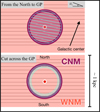 |
Fig. 6 Sketch of the toy model showing the LB and the mean magnetic field in the solar neighborhood from the north pole to the Galactic plane (GP, top) and across the GP (bottom). Dark colors correspond to structures of CNM, light colors to the WNM, cyan lines to magnetic-field lines in the CNM, and purple lines to the magnetic-field lines of the WNM. The Sun position in the LB is represented by a red-white circle. An inset in the top panel shows the angle δli between the LB/CNM field and the mean/WNM magnetic field. |
5.2.1 Geometrical toy model of the magnetic field
We aim to model the misalignment angle specifically at the largest angular scales (ℓ < 20), which are most relevant for the observed misalignment between dust polarization and the H I templates (see Fig. 5). For this purpose, we utilize the phenomenological multi-layer model introduced by Planck Collaboration Int. XLIV (2016), which has been applied in several studies to fit the Planck data at high Galactic latitudes (e.g., Vansyngel et al. 2017; Planck Collaboration Int. L 2017) and to model the rotation measure maps of the LB using the LOw Frequency ARray (LOFAR, e.g., Boulanger et al. 2024).
In this work, we just considered the regular (ordered) magnetic field vector B0 as we are interested in the line-of-sight geometrical variation of the magnetic field at large angular scales. We do not include any curvature term in the ordered component. Moreover, since we focus on angle differences, our model only depends on the direction of  , which is assumed to be uniform and pointing toward Galactic coordinates (l0, b0), such that its coordinates are (cos l0cos b0, sin l0cos b0, sin b0). Defining the generic line-of-sight unit vector
  as (cos l cos b, sin l cos b, sin b), the line-of-sight
  and plane-of-the-sky
  components of
  can be expressed as
 (4)
(4)
From Eq. (4), we computed the geometric parts of the Stokes parameters, q ∝ Q/I and u ∝ U/I, corresponding to  as
as
 (5)
(5)
The parameter γ0 is the angle between the magnetic field and the plane of the sky; the parameter ψ0 is the polarization angle. These two angles are defined as
 (6)
(6)
where  is the unit vector perpendicular to
  within the
  plane and
  is the unit vector pointing toward the north Galactic pole in Galactic coordinates.
This toy model produces a map of ψ0 that in our scenario corresponds to the polarization angle of the regular magnetic field traced by the WNM. To introduce the impact of the LB, we imposed that, at large scales, the direction of  in the two hemispheres corresponds to a rotation of
  , such that
  points toward Galactic coordinates (l0 + δli, b0 + δbi) with the index "i" referring to either the southern or northern hemisphere (see cyan lines in the LB and top-right inset in Fig. 6). Using Eqs. (4–6) in the case of
  , we derived the corresponding geometrical parts of Stokes parameters qLB and uLB representing the magnetic field on the LB surface traced by the CNM.
The final step of our geometrical approach is the derivation of the total Stokes parameters, which, in terms of their geometrical parts, are modeled as
 (7)
(7)
where fL represents the relative contribution of the LB to the total polarization signal. Finally, using Eq. (2), we computed the misalignment angle between ψtot, a proxy of dust polarization, and ψLB, a proxy of the H I templates, in the 20% mask. We notice that the strongest impact on the misalignment angle in this sky area is determined by δli compared to δbi. Thus, fixing δbi = 0°, in the models, we explored the effect on the observed misalignment angle of changing δli (the intrinsic misalignment and fL.
We fixed (l0, b0) = (72.5°, −5°) to be an intermediate direction with respect to those found by Pelgrims et al. (2020) in the southern and northern hemispheres (see Sect. 5.2). In Fig. 7, we show how the misalignment angle varies as a function of fL (see colors) for both hemispheres (see diagonal perpendicular hatches) given δli = ±12° in the southern and northern hemispheres, respectively. With light-gray shades, we also show the case with δli = +12° in both hemispheres.
We observe that only tilted distortion of the LB field compared to the regular field (see Fig. 6) or a change in sign of δli between the two Galactic hemispheres can reproduce the same hemispherical sign of misalignment angle observed in the data. This may correspond to the distortion of the regular field caused by the LB similar to an effective large-scale helical component of the magnetic field, as proposed by Bracco et al. (2019a). We also note that, despite having δli = ±12°, the observed misalignment angle can be significantly smaller depending on fL. Specifically, it ranges from 0° to 12° depending on whether the LB completely dominates the total polarization signal (fL = 1) or is negligible compared to the regular-field contribution (fL = 0). In Fig. 8, we further explore this by varying both fL and |δli| and applying opposite signs in the two hemispheres. Our models demonstrate that even with large values of |δli| (e.g., |δli| > 50°) the observed misalignment may be negligible depending on fL. With black contours we draw the levels of misalignment observed in the data between 5° and 10°.
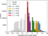 |
Fig. 7 Modeled misalignment angle between the LB magnetic field and the total one as a function of fL. Hatches show the misalignment in each Galactic hemisphere separately. As an example, the intrinsic misalignment angle δli is ±12° in the southern and northern hemisphere, respectively. The histograms were computed in the 20% mask. In light gray, the cases for both hemispheres with δli = +12° are shown. |
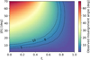 |
Fig. 8 Dependence of the observed misalignment angle with fL and |δli| in the toy model. Black contours show levels of misalignment angle similar to what was measured in the Planck data. |
5.2.2 Synchrotron misalignment
These models predict that the misalignment with the H I templates should increase for datasets with less contribution from the LB, i.e., when fL is smaller than for dust polarization. This hypothesis is supported by Planck polarization data at 30 GHz, which predominantly traces synchrotron radiation. Given that the synchrotron scale height in spiral galaxies is generally larger than that of the dusty disk over scales of a few hundred parsecs (e.g., Beck 2015), synchrotron radiation is expected to have a smaller fL compared to the dusty case, that is, the contribution of the regular magnetic field should be more important (Pelgrims et al. 2025). In Fig. B.2, the NPDFs of Δψ using Planck data at 30 GHz are shown with the respective values of 〈Δψ〉circ as a function of ℓFWHM. Both hemispheres exhibit the same sign of large-scale misalignment as observed with dust, but with significantly larger values of 〈Δψ〉circ aligning with the model expectations. Furthermore, the scale dependence of 〈Δψ〉circ in the two hemispheres, similar to that observed for dust, is particularly notable in the case of synchrotron radiation. While there is little dependence on ℓFWHM in the northern hemisphere, an abrupt change in misalignment is observed in the southern hemisphere. These features highlight the multi-scale complexity of the misalignment, which our simplified model does not fully capture. A more detailed comparison of synchrotron and dust polarization would be important but is beyond the scope of this work.
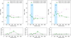 |
Fig. 9 Misalignment angle between polarization data (rotated by 90°) and starlight polarization measurements as a function of the stellar distance for Planck data at 353 GHz (top-left panel), H I polarization templates (top-central panel), and Planck data at 30 GHz (top-right panel). The misalignment is shown in green and pink for the northern and southern he mispheres, respectively. The misalignment peaks at the edge of the LB in cyan. With the same color scheme, the bottom panels show the average normalized kurtosis of the corresponding Δψ distributions. The uncertainty is the standard deviation between the two versions of each dataset. The gray shaded area represents the standard deviation of the average kurtosis of a normal distribution in the case of low-number statistics, as for the number of stars per distance bin (approximately 20). |
5.2.3 Starlight polarization: Distance dependence
The geometrical toy model suggests that the misalignment angle should also depend on the heliocentric distance to the magnetic field responsible for the dust polarization signal. We explored this idea using the starlight polarization catalog described in Sect. 2.3. We computed the misalignment angle between starlight polarization angles and the Planck data at 353 GHz, the H I templates, and the Planck data at 30 GHz. This was obtained in the 20% mask by sampling the starlight measurements in seven distance bins within 1 kpc from the Sun. The total number of selected stars is 306, corresponding to 86% of the original catalogs of Heiles (2000), Berdyugin & Teerikorpi (2001), Berdyugin & Teerikorpi (2002), and Berdyugin et al. (2014).
We applied Eq. (2) after projecting the starlight measurements on a HEALPix grid at Nside = 128. Before computing the misalignment angle, we averaged the Stokes parameters of those stars with Galactic coordinates falling in the same HEALPix pixels. However, given the sparsity of stars at high Galactic latitudes (see Fig. C.1), this averaging effect did not strongly impact the results, as it involved multiple counting for only 3% of the sample. We note that stellar sparsity also represents a potential systematic bias in estimating large-scale polarization fields using stars, as some coherence from small to large scales must be assumed.
We computed the misalignment angle for the northern and southern hemispheres, separately. The number of bins was chosen to have a roughly homogeneous number of stars per bin while also sampling the distance range between a few tens to hundreds of parsecs. The upper limits of each bin were 120, 150, 190, 250, 300, 420, and 1000 pc. With 208 and 98 stars in the northern and southern Galactic hemispheres, respectively, seven distance bins guaranteed, on average, 30 and 14 stars per bin in the two hemispheres.
In Fig. 9, we show the misalignment angle between starlight polarization and the other tracers as a function of the average stellar distance per bin. Error bars on the y axis represent systematic effects of Planck and H I data and the dispersion of the starlight polarization angles. On the X axis, the error bars indicate the distance width of each bin. In the bottom row of the same figure, we display the kurtosis of the corresponding NPDFs averaged between two versions of the same dataset (e.g., PR4 and SRoll2 in the case of Planck data at 353 GHz). The normalized kurtosis provide us with an indication on how much the NPDFs are peaked. The gray-shaded areas represent the standard deviation of the average kurtosis of a normal distribution. Apart from the first distance bin, all NPDFs are well-peaked around the value of 〈Δψ〉circ plotted in the top row of Fig. 9.
We observe that, at 353 GHz, a misalignment angle on the order of 7°, which is consistent with Fig. 2, is found at the distance of the LB wall, namely, between 100 and 200 pc at high Galactic latitude (e.g., Pelgrims et al. 2020; O'Neill et al. 2024). The misalignment disappears at larger distances, in agreement with Skalidis & Pelgrims (2019). Probably because of better number statistics, this effect is clearer in the northern hemisphere than in the southern hemisphere. However, this could also be a physical effect as illustrated by the hemispherical difference in Figs. 2 and 4.
As predicted by the geometrical model in Sect. 5.2.1, starlight polarization and Planck data at 353 GHz are sensitive to the same magnetic-field structure only at large heliocentric distances; at smaller distances, stars are sensitive to the LB/CNM field revealed by the misalignment. This is supported by the misalignment angle between stars and the Η I templates. Starlight polarization angles show no misalignment with the H I templates at the distance of the LB wall but reveal a flat misalignment at further distances, consistent with dust polarization in emission.
Finally, we observe a stronger positive misalignment between starlight polarization and Planck data at 30 GHz in both hemispheres. This misalignment vanishes more slowly with distance compared to the Planck data at 353 GHz in the northern hemisphere, and it remains roughly constant in the southern hemisphere. Understanding these differences in detail is beyond the scope of the present paper; however we speculate that they may be related to a generally more coherent magnetic-field structure along the line of sight in the northern area sampled by the stellar measurements. These results are consistent with the proposed scenario, where the 30-GHz data would more efficiently trace the regular magnetic-field component compared to the LB field, implying a smaller value of fL, thus a stronger misalignment angle. In summary, starlight polarization data support our phase superposition scenario as follows:
At the location of the LB, stars mostly trace CNM and its magnetic field while dust emission also includes the WNM-weighted field on larger scales, producing misalignment. At large distances, stars additionally probe the WNM-weighted magnetic field and begin converging to the dust emission.
Complementary to the previous case, H I templates correlate with starlight polarization at the location of the LB and depart from it at larger distances.
The typical scale height is larger for synchrotron than for dust. Because synchrotron mostly traces the mean field on scales larger than the LB (low value of /L), it shows a strong misalignment with stars at the position of the LB and only correlates with starlight polarization at very large distances in the northern hemisphere, where the magnetic-field structure may be generally more coherent in the area sampled by the stars.
A denser sample of stars, with defined distances and polarization measurements, will be essential for a better investigation of our scenario regarding the misalignment angle. Projects such as the Polar-Areas Stellar Imaging in Polarization High-Accuracy Experiment (PASIPHAE, Tassis et al. 2018), which will increase the number of studied stars a thousandfold over the current state of the art at intermediate and high Galactic latitudes, are expected to be transformative.
5.3 Impact on dust polarization angular power spectra
We now discuss the link between the observed large-scale misalignment and the dust polarization angular power spectra, particularly focusing on the observed T B correlation in the Planck data (Planck Collaboration XI 2020). We first present the Planck T B power spectra at 353 GHz for the two Galactic hemispheres and then demonstrate how the signal can be suppressed by removing the large-scale contribution (Sect. 5.3.1).
In its current form, our model (see Sect. 5.2.1) does not reproduce Τ Β cross-spectra. Future work is needed in order to include multiscale filamentary intensity models that must correlate with the 3D magnetic-field structure as in the geometrical model described in this work and similar to the case study of line-of-sight superposition presented in Vacher et al. (2023). Another possibility could be to look at realistic MHD simulations in projections, as initiated in previous works (e.g., Clark et al. 2021; Pelgrims et al. 2022; Maconi et al. 2023). Nevertheless, in Sect. 5.3.2, we use synthetic filamentary models in 2D, as described in Appendix E, to illustrate the effect of a coherent large-scale misalignment on the small-scale Τ Β correlation.
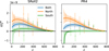 |
Fig. 10 Planck Τ Β power spectra in the northern and southern Galactic hemispheres. Power spectra were computed in the 20% mask with both SRoll2 and PR4 maps. Units are in |

5.3.1 Hemispherical look at the Planck data
In Fig. 10, we show the T B power spectra, defined as 𝒟T Bℓ = ℓ(ℓ + 1)CT Bℓ/2π and computed in the 20% mask for the northern and southern Galactic hemispheres. The details of the power-spectrum calculation are provided in Appendix D. Using both SRoll2 (left panel) and PR4 data (right panel), the spectra are averaged with a linear multipole binning starting at ℓ = 5 (shown as data points). Best-fit power-laws with a beam roll-off are also displayed, with shaded regions indicating the 1σ uncertainty. The northern hemisphere consistently exhibits a stronger positive Τ Β correlation than the southern hemisphere.
A similar hemispherical split was performed in Cukierman et al. (2023), which focused mainly on higher multipoles (ℓ > 100) and larger sky areas (e.g., fsky = 70%). In fig. 11, Cukierman et al. (2023) provides a misalignment estimate based on TdBd (labeled "Dust only") for the 20% mask and the associated hemispherical splits, though the scales have been limited to ℓ > 100. As in Fig. 10, the north yields a signal that is moderately strong, and the south yields a result that is consistent with zero.
This hemispherical difference is consistent with the expectations from the misalignment analysis, where a stronger and more coherent large-scale misalignment angle is found in the north (see also Fig. D.1). To further establish the connection, we recomputed the spectra after de-rotating the large-scale misalignment, which is measured from the angle differences between smoothed Planck polarization maps and smoothed H I templates. This calculation uses Eqs. 2 and 3 with ℓref = 20. In Fig. 11, we show the original and de-rotated power spectra; for the latter, we consider both Η I templates, namely, the Hessian and the SRHT. In both cases, we are able to suppress the Τ Β correlation in the north by accounting only for the large-scale dust-Η I misalignment. We stress that the de-rotation, which is based only on large-scale information (ℓref = 20), is able to suppress the T B correlation even at small scales (ℓ > 200). Finally, we notice that hemispherical differences are also found with other tracers of the multiphase and magnetized ISM, such as rotation-measure patterns at large angular scales, whose origin remains unclear (e.g., Dickey et al. 2022; Booth et al. 2026).
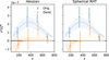 |
Fig. 11 Planck T B power spectra from both Galactic hemispheres with the 20% mask before and after de-rotation, using SRoll2 for the dust maps and two different H I templates. The de-rotation was computed at ℓref = 20. Units are |

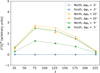 |
Fig. 12 Modeled T B power spectra as a function of the misalignment angles ΔψN and ΔψS in the north and south Galactic hemispheres, respectively. Power spectra were computed with the 20% mask. |
5.3.2 Insights from 2D synthetic filamentary models
As described in Appendix E, we built synthetic maps to test the impact of a large-scale misalignment on the Τ Β correlation at small scales. The synthetic maps include a filamentary model perfectly aligned to the magnetic field orientation, to which we add two uniform effective misalignment angles projected on the plane of the sky, ΔψΝ and ΔψS, in the two Galactic hemispheres. These two components correspond to the LB magnetic field and the total one as described by the geometrical model in Sect. 5.2.1. From the synthetic Stokes IQU, we compute  in arbitrary units within the 20% mask using the healpy package. Rather than fitting the data, our goal is to gain intuition on the effects of the geometrical model on the polarization power spectra. As shown in Fig. 12, by setting different values of ΔψΝ and ΔψS at the largest scales (uniform over each Galactic hemisphere), we can control the level of Τ Β correlation over a wide range of multipoles. Only by setting the same sign for ΔψΝ and ΔψS6 can we achieve the same sign of
  in the two hemispheres. This effective tilt of the LB field could be analogous to the large-scale helical magnetic field proposed by Bracco et al. (2019a) to reproduce the observed Τ Β signal.
6 Summary and conclusion
We have presented new data analyses and one physical scenario to gain insight into the origin of two observables of the dusty, polarized sky at intermediate and high Galactic latitudes: (1) the statistical misalignment between atomic hydrogen (H I) filamentary structures and dust polarization angles and (2) the T B correlation detected in Planck polarization data. Using a multiwavelength analysis of Planck data at 30, 217, and 353 GHz as well as starlight polarization measurements and H I-based templates, we showed that both phenomena are stronger at large scale and in the northern Galactic hemisphere. The misalignment could be interpreted as a consequence of large-scale line-of-sight projection effects on the magnetic-field structure sampled by different ISM phases in the solar neighborhood. In power spectra, this large angular scale effect could be inherited by small scales, which have been considered responsible for both observables (e.g., Huffenberger et al. 2020; Hervías-Caimapo & Huffenberger 2022; Clark et al. 2021; Cukierman et al. 2023; Hervías-Caimapo et al. 2025). The key results of this work are the following:
The misalignment angle in the 20% of the sky at high Galactic latitude is significant mainly on large angular scales (ℓ ≤ 20) and varies between the two Galactic hemispheres, with the northern hemisphere showing a larger and more coherent misalignment. This result holds true at all Planck frequencies considered in this work, being stronger at lower frequencies in the synchrotron domain.
We showed that the misalignment is unlikely to be related to dust emissivity variations and can be reproduced with a two-layer geometrical toy model where the large-scale regular magnetic field in the solar neighborhood is distorted by the LB. The LB induces a relative tilt between CNM- and WNM-traced magnetic fields, which in projection produces the misalignment and, possibly, the T B correlation. The observed distance dependence of the misalignment, traced with starlight polarization measurements, supports this interpretation for the misalignment.
As a consequence of the proposed scenario, H I filamentary structures can be considered statistically aligned with magnetic fields in the diffuse ISM, in agreement with hydro-magnetic turbulence, although some caution is needed. The projected scatter around the mean remains significant, on the order of a few tens of degrees. Future work will be necessary to clarify the physical origin of this scatter.
We presented T B power spectra of Planck data at 353 GHz for the two Galactic hemispheres. We found that the Τ Β correlation is stronger at large scales and mostly in the northern hemisphere, consistent with the misalignment analysis. By de-rotating the Stokes parameters to account for the large-scale misalignment between the Planck data and Η I templates (ℓ ≤ 20), we were able to consistently suppress the observed Τ Β correlation at small scales (ℓ > 100). This de-rotation is more effective in the northern hemisphere than in the southern, where the scale dependence of the misalignment angle suggests a more complex physical scenario.
Although we could not reproduce the complexity of the Τ Β correlation with the toy model detailed in Sect. 5.2.1, using synthetic 2D filamentary sky models we demonstrated that a large-scale misalignment can produce a small-scale T B correlation.
Our results emphasize the critical role of large-scale structures in the solar neighborhood in shaping polarized Galactic signals. This has important implications for both Galactic magnetic-field studies and future CMB polarization experiments.
Acknowledgements
The authors acknowledge the Interstellar Institute's programs "II6" & "II7" and the Paris-Saclay University's Institut Pascal for hosting discussions that nourished the development of the ideas behind this work. This work was supported by NSF grant AST-2109127. A.B. acknowledges financial support from the INAF initiative "IAF Astronomy Fellowships in Italy" (grant name MEGASKAT). This work is a tribute to the imagination of my beloved uncle Pasquale: "So be it, heart; bid farewell without end" [H. Hesse]. R.S. was supported by NASA through the NASA Hubble Fellowship grant HST-HF2-51566.001 awarded by the Space Telescope Science Institute, which is operated by the Association of Universities for Research in Astronomy, Inc., for NASA, under contract NAS5-26555. We are thankful to Vincent Pelgrims, Susan Clark, Antoine Marchal, Pierre Lesaffre, and Tuhin Ghosh for insightful discussions. We thank Matthew A. Price for helping us with the S2WAV package. Some of the results in this paper have been derived using the healpy and HEALPix packages. In the analysis we made use of astropy (Astropy Collaboration 2018), scipy (Virtanen et al. 2020), and numpy (Harris et al. 2020).
References
- Adak, D., Ghosh, T., Boulanger, F., et al. 2020, A&A, 640, A100 [NASA ADS] [CrossRef] [EDP Sciences] [Google Scholar]
- Alonso, D., Sanchez, J., Slosar, A., & LSST Dark Energy Science Collaboration. 2019, MNRAS, 484, 4127 [NASA ADS] [CrossRef] [Google Scholar]
- Alves, M. I. R., Boulanger, F., Ferrière, K., & Montier, L. 2018, A&A, 611, L5 [NASA ADS] [CrossRef] [EDP Sciences] [Google Scholar]
- André, P., Men'shchikov, A., Bontemps, S., et al. 2010, A&A, 518, L102 [CrossRef] [EDP Sciences] [Google Scholar]
- Astropy Collaboration (Price-Whelan, A. M., et al.) 2018, AJ, 156, 123 [Google Scholar]
- Beck, R. 2015, A&A Rev., 24, 4 [Google Scholar]
- Berdyugin, A., & Teerikorpi, P. 2001, A&A, 368, 635 [NASA ADS] [CrossRef] [EDP Sciences] [Google Scholar]
- Berdyugin, A., & Teerikorpi, P. 2002, A&A, 384, 1050 [NASA ADS] [CrossRef] [EDP Sciences] [Google Scholar]
- Berdyugin, A., Piirola, V., & Teerikorpi, P. 2014, A&A, 561, A24 [NASA ADS] [CrossRef] [EDP Sciences] [Google Scholar]
- BICEP2/Keck, & Planck Collaborations 2015, Phys. Rev. Lett., 114, 101301 [Google Scholar]
- Booth, R. A., Ordog, A., Brown, J.-A., et al. 2026, ApJ, 997, 304 [Google Scholar]
- Boulanger, F., Abergel, A., Bernard, J. P., et al. 1996, A&A, 312, 256 [Google Scholar]
- Boulanger, F., Gry, C., Jenkins, E. B., et al. 2024, A&A, 687, A102 [NASA ADS] [CrossRef] [EDP Sciences] [Google Scholar]
- Bracco, A., Candelaresi, S., Del Sordo, F., & Brandenburg, A. 2019a, A&A, 621, A97 [NASA ADS] [CrossRef] [EDP Sciences] [Google Scholar]
- Bracco, A., Ghosh, T., Boulanger, F., & Aumont, J. 2019b, A&A, 632, A17 [NASA ADS] [CrossRef] [EDP Sciences] [Google Scholar]
- Clark, S. E., & Hensley, B. S. 2019, ApJ, 887, 136 [NASA ADS] [CrossRef] [Google Scholar]
- Clark, S. E., Hill, J. C., Peek, J. E. G., Putman, M. E., & Babler, B. L. 2015, Phys. Rev. Lett., 115, 241302 [Google Scholar]
- Clark, S. E., Kim, C.-G., Hill, J. C., & Hensley, B. S. 2021, ApJ, 919, 53 [NASA ADS] [CrossRef] [Google Scholar]
- Clark, S. E., Peek, J. E. G., & Miville-Deschênes, M. A. 2019, ApJ, 874, 171 [NASA ADS] [CrossRef] [Google Scholar]
- Cukierman, A. J., Clark, S. E., & Halal, G. 2023, ApJ, 946, 106 [Google Scholar]
- Davis, L., Jr., & Greenstein, J. L. 1951, ApJ, 114, 206 [NASA ADS] [CrossRef] [Google Scholar]
- Delouis, J. M., Pagano, L., Mottet, S., Puget, J. L., & Vibert, L. 2019, A&A, 629, A38 [NASA ADS] [CrossRef] [EDP Sciences] [Google Scholar]
- Dickey, J. M., West, J., Thomson, A. J. M., et al. 2022, ApJ, 940, 75 [NASA ADS] [CrossRef] [Google Scholar]
- Eskilt, J. R., & Komatsu, E. 2022, Phys. Rev. D, 106, 063503 [NASA ADS] [CrossRef] [Google Scholar]
- Ferrière, K. 2020, Plasma Phys. Controlled Fusion, 62, 014014 [CrossRef] [Google Scholar]
- Ghosh, T., Boulanger, F., Martin, P. G., et al. 2017, A&A, 601, A71 [NASA ADS] [CrossRef] [EDP Sciences] [Google Scholar]
- Górski, K. M., Hivon, E., Banday, A. J., et al. 2005, ApJ, 622, 759 [Google Scholar]
- Grain, J., Tristram, M., & Stompor, R. 2009, Phys. Rev. D, 79, 123515 [Google Scholar]
- Guillet, V., Fanciullo, L., Verstraete, L., et al. 2018, A&A, 610, A16 [NASA ADS] [CrossRef] [EDP Sciences] [Google Scholar]
- Hacar, A., Clark, S. E., Heitsch, F., et al. 2023, ASP Conf. Ser., 534, 153 [NASA ADS] [Google Scholar]
- Halal, G., Clark, S. E., Cukierman, A., Beck, D., & Kuo, C.-L. 2024, ApJ, 961, 29 [Google Scholar]
- Harris, C. R., Millman, K. J., van der Walt, S. J., et al. 2020, Nature, 585, 357 [NASA ADS] [CrossRef] [Google Scholar]
- Heiles, C. 2000, AJ, 119, 923 [Google Scholar]
- Hervías-Caimapo, C., Cukierman, A. J., Diego-Palazuelos, P., Huffenberger, K. M., & Clark, S. E. 2025, Phys. Rev. D, 111, 083532 [Google Scholar]
- Hervías-Caimapo, C., & Huffenberger, K. M. 2022, ApJ, 928, 65 [CrossRef] [Google Scholar]
- HI4PI Collaboration (Ben Bekhti, N., et al.) 2016, A&A, 594, A116 [NASA ADS] [CrossRef] [EDP Sciences] [Google Scholar]
- Hildebrand, R. H. 1988, Astrophys. Lett. Commun., 26, 263 [Google Scholar]
- Hiltner, W. A. 1949, Nature, 163, 283 [CrossRef] [Google Scholar]
- Hoang, T., Cho, J., & Lazarian, A. 2018, ApJ, 852, 129 [NASA ADS] [CrossRef] [Google Scholar]
- Huffenberger, K. M., Rotti, A., & Collins, D. C. 2020, ApJ, 899, 31 [NASA ADS] [CrossRef] [Google Scholar]
- Inoue, T., & Inutsuka, S. 2016, ApJ, 833, 10 [Google Scholar]
- Inutsuka, S.-I., Inoue, T., Iwasaki, K., & Hosokawa, T. 2015, A&A, 580, A49 [NASA ADS] [CrossRef] [EDP Sciences] [Google Scholar]
- Komatsu, E. 2022, Nat. Rev. Phys., 4, 452 [NASA ADS] [CrossRef] [Google Scholar]
- Lee, H. M., & Draine, B. T. 1985, ApJ, 290, 211 [Google Scholar]
- Lenz, D., Hensley, B. S., & Doré, O. 2017, ApJ, 846, 38 [NASA ADS] [CrossRef] [Google Scholar]
- Lue, A., Wang, L., & Kamionkowski, M. 1999, Phys. Rev. Lett., 83, 1506 [NASA ADS] [CrossRef] [Google Scholar]
- Maconi, E., Soler, J. D., Reissl, S., et al. 2023, MNRAS, 523, 5995 [NASA ADS] [CrossRef] [Google Scholar]
- Mandarakas, N., Tassis, K., & Skalidis, R. 2025, A&A, 698, A168 [NASA ADS] [CrossRef] [EDP Sciences] [Google Scholar]
- Marchal, A., & Miville-Deschênes, M.-A. 2021, ApJ, 908, 186 [NASA ADS] [CrossRef] [Google Scholar]
- Marchal, A., Martin, P. G., Miville-Deschênes, M.-A., et al. 2024, ApJ, 961, 161 [NASA ADS] [CrossRef] [Google Scholar]
- Miville-Deschênes, M. A., & Martin, P. G. 2007, A&A, 469, 189 [NASA ADS] [CrossRef] [EDP Sciences] [Google Scholar]
- O'Neill, T. J., Zucker, C., Goodman, A. A., & Edenhofer, G. 2024, ApJ, 973, 136 [NASA ADS] [CrossRef] [Google Scholar]
- Panopoulou, G. V., Markopoulioti, L., Bouzelou, F., et al. 2025, ApJS, 276, 15 [NASA ADS] [CrossRef] [Google Scholar]
- Pelgrims, V., Ferrière, K., Boulanger, F., Lallement, R., & Montier, L. 2020, A&A, 636, A17 [EDP Sciences] [Google Scholar]
- Pelgrims, V., Clark, S. E., Hensley, B. S., et al. 2021, A&A, 647, A16 [NASA ADS] [CrossRef] [EDP Sciences] [Google Scholar]
- Pelgrims V. Ntormousi E. & Tassis K. 2022 A&A 658 A134 [NASA ADS] [CrossRef] [EDP Sciences] [Google Scholar]
- Pelgrims, V., Unger, M., & Mariş, I. C. 2025, A&A, 695, A148 [NASA ADS] [CrossRef] [EDP Sciences] [Google Scholar]
- Pineda, J. E., Arzoumanian, D., Andre, P., et al. 2023, ASP Conf. Ser., 534, 233 [NASA ADS] [Google Scholar]
- Planck Collaboration I. 2020, A&A, 641, A1 [NASA ADS] [CrossRef] [EDP Sciences] [Google Scholar]
- Planck Collaboration XI. 2020, A&A, 641, A11 [NASA ADS] [CrossRef] [EDP Sciences] [Google Scholar]
- Planck Collaboration XII. 2020, A&A, 641, A12 [NASA ADS] [CrossRef] [EDP Sciences] [Google Scholar]
- Planck Collaboration Int. XX. 2015, A&A, 576, A105 [NASA ADS] [CrossRef] [EDP Sciences] [Google Scholar]
- Planck Collaboration Int. XXX. 2016, A&A, 586, A133 [NASA ADS] [CrossRef] [EDP Sciences] [Google Scholar]
- Planck Collaboration Int. XXXII. 2016, A&A, 586, A135 [NASA ADS] [CrossRef] [EDP Sciences] [Google Scholar]
- Planck Collaboration Int. XXXV. 2016, A&A, 586, A138 [NASA ADS] [CrossRef] [EDP Sciences] [Google Scholar]
- Planck Collaboration Int. XXXVIII. 2016, A&A, 586, A141 [NASA ADS] [CrossRef] [EDP Sciences] [Google Scholar]
- Planck Collaboration Int. XLIV. 2016, A&A, 596, A105 [NASA ADS] [CrossRef] [EDP Sciences] [Google Scholar]
- Planck Collaboration Int. XLIX. 2016, A&A, 596, A110 [NASA ADS] [CrossRef] [EDP Sciences] [Google Scholar]
- Planck Collaboration Int. L. 2017, A&A, 599, A51 [NASA ADS] [CrossRef] [EDP Sciences] [Google Scholar]
- Planck Collaboration Int. LVII. 2020, A&A, 643, A42 [NASA ADS] [CrossRef] [EDP Sciences] [Google Scholar]
- Price, M. A., & McEwen, J. D. 2024, J. Comput. Phys., 510, 113109 [Google Scholar]
- Price, M. A., Polanska, A., Whitney, J., & McEwen, J. D. 2024, arXiv e-prints [arXiv:2402.01282] [Google Scholar]
- Reissl, S., Guillet, V., Brauer, R., et al. 2020, A&A, 640, A118 [NASA ADS] [CrossRef] [EDP Sciences] [Google Scholar]
- Ritacco, A., Boulanger, F., Guillet, V., et al. 2023, A&A, 670, A163 [NASA ADS] [CrossRef] [EDP Sciences] [Google Scholar]
- Ritacco, A., Bizzarri, L., Savorgnano, S., et al. 2024, PASP, 136, 115001 [Google Scholar]
- Robitaille, J. F., Abdeldayem, A., Joncour, I., et al. 2020, A&A, 641, A138 [NASA ADS] [CrossRef] [EDP Sciences] [Google Scholar]
- Skalidis, R. 2024, A&A, submitted [arXiv:2411.08971] [Google Scholar]
- Skalidis, R., & Pelgrims, V. 2019, A&A, 631, L11 [NASA ADS] [CrossRef] [EDP Sciences] [Google Scholar]
- Soler, J. D., & Hennebelle, P. 2017, A&A, 607, A2 [NASA ADS] [CrossRef] [EDP Sciences] [Google Scholar]
- Tassis, K., & Pavlidou, V. 2015, MNRAS, 451, L90 [NASA ADS] [CrossRef] [Google Scholar]
- Tassis, K., Ramaprakash, A. N., Readhead, A. C. S., et al. 2018, arXiv e-prints [arXiv:1810.05652] [Google Scholar]
- Tram, L. N., Hoang, T., Wiesemeyer, H., et al. 2024, A&A, 689, A290 [NASA ADS] [CrossRef] [EDP Sciences] [Google Scholar]
- Vacher, L., Aumont, J., Boulanger, F., et al. 2023, A&A, 672, A146 [NASA ADS] [CrossRef] [EDP Sciences] [Google Scholar]
- Vansyngel, F., Boulanger, F., Ghosh, T., et al. 2017, A&A, 603, A62 [NASA ADS] [CrossRef] [EDP Sciences] [Google Scholar]
- Virtanen, P., Gommers, R., Oliphant, T. E., et al. 2020, Nat. Methods, 17, 261 [Google Scholar]
- Wardle, M., & Konigl, A. 1990, ApJ, 362, 120 [NASA ADS] [CrossRef] [Google Scholar]
- Weiland, J. L., Addison, G. E., Bennett, C. L., Halpern, M., & Hinshaw, G. 2020, ApJ, 893, 119 [NASA ADS] [CrossRef] [Google Scholar]
- Wolfire, M. G., McKee, C. F., Hollenbach, D., & Tielens, A. G. G. M. 2003, ApJ, 587, 278 [Google Scholar]
- Zaldarriaga, M. 2001, Phys. Rev. D, 64, 103001 [NASA ADS] [CrossRef] [Google Scholar]
- Zaldarriaga, M., & Seljak, U. c. v. 1997, Phys. Rev. D, 55, 1830 [Google Scholar]
- Zonca, A., Singer, L., Lenz, D., et al. 2019, J. Open Source Softw., 4, 1298 [Google Scholar]
- Zucker, C., Goodman, A. A., Alves, J., et al. 2022, Nature, 601, 334 [NASA ADS] [CrossRef] [Google Scholar]
The circular, or angular, mean is a directional statistic that differs from a standard mean as it applies to cyclical quantities.
This is the standard error on the mean.
Given the plane-of-the-sky projection and the 3D modeling, the same sign between ΔψΝ and ΔψS corresponds to opposite signs in the case of δli.
The complete Python routine used in this work, dirade_hpx (Directional RAndom cascaDE in HEALPix), can be found at http://github.com/abracco/cosmicodes/blob/master/4GMIMS/Planck_routines.py.
Appendix A Sky maps
As described in Sect. 3, Fig. A.1 shows an example of rotating the Stokes parameters with respect to a larger-scale reference set by ℓref = 20. The rotation obtained with Eq. 3 is applied on Q353,d and U353,d from SRoll2. We applied the 80% mask. After rotation, it can be noticed that most of the polarization signal is converted, by construction, to positive values of  , while
  resembles a dispersion around the mean. In this reference frame, the polarization angle, shown with the line integral convolution (LIC) function of healpy in the bottom row, is essentially perpendicular to the Galactic plane and the magnetic field orientation parallel to it.
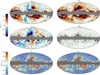 |
Fig. A.1 Effect of the angle rotation on the Planck Stokes parameters using Eq. 3. The original data at FWHM=80' are shown in the left column and the maps rotated with respect to ℓref = 20 in the right column. The Stokes parameters are shown in the top and central panels with the same color bar displayed on the left, while polarized intensities are shown in the bottom panels in the background of the drapery patterns tracing the magnetic-field orientation obtained through LIC. The 80% sky mask is applied (see Fig. 1). |
Appendix B Misalignment angle at 217 and 30 GHz
In this appendix, we show the NPDFs of the misalignment angle as a function of ℓFWHM between the H I templates and the Planck data at 217 and 30 GHz, respectively. The former is shown in Fig. B.1, and the latter in Fig. B.2. In both cases we found a strong large-scale misalignment as in the case of Planck data at 353 GHz. Refer to Sect. 5.1 and Sect. 5.2.1 for more details.
Appendix C Starlight measurements on the sky
This appendix shows the distribution of starlight measurements in the 20% mask with an orthographic projection around the two Galactic poles. In Fig. C.1, the star hits are displayed, with only 3% of pixels counting two selected stars in the stellar catalog at Nside = 128.
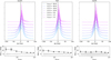 |
Fig. B.1 Same as for Fig. 4 but considering Planck data at 217 GHz as a test of the robustness of the results for 353 GHz. A similar misalignment as at 353 GHz is also found at 217 GHz. |
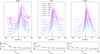 |
Fig. B.2 Same as for Fig. 4 but considering Planck data at 30 GHz, which is dominated by synchrotron radiation rather than dust emission. A stronger misalignment than at 353 GHz is found at 30 GHz, where synchrotron polarization is traced. |
Appendix D Computing TB power spectra
Angular power spectra Q are computed with NaMaster (Alonso et al. 2019). Our sky masks are apodized with a C2 window (Grain et al. 2009) with a scale of 1°. For the computation of power spectra, different from what is described in Sect. 2, all of our maps are smoothed to 40' and downgraded to Nside = 256 in HEALPix format (Górski et al. 2005). Our power spectra are computed in the TEB basis (e.g., Zaldarriaga & Seljak 1997), and we are mainly interested in the TB cross spectrum.
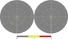 |
Fig. C.1 Orthographie projection around the northern (left) and southern (right) Galactic poles of the hit map of stars after reprojecting the measurements on a HEALPix grid at Nside = 128. A galactic coordinate grid is overlaid. |
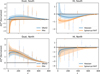 |
Fig. D.1 Estimates of Τ Β cross spectra for dust and Η I filaments in the two Galactic hemispheres with the 20% mask. This is a comparison between the various spectra depending on the given Planck dataset (left, TdB353) and Η I template (right, TdBHI). To be able to compare all of these quantities, which have different physical units, we have normalized each spectrum to the mean of its absolute values. |
In Fig. D.1, we present the T B power spectra for four distinct cases in the form of Dℓ = ℓ(ℓ + 1)Cℓ/2π. The analysis separates the two Galactic hemispheres, and the input QU Stokes parameters are derived either from Planck data at 353 GHz or from the Η I templates. For the intensity map, we consider only Id (hereafter Td, see Sect. 2.1). To assess the impact of systematic effects, we compute the power spectra using two versions of each dataset (e.g., SRoll2 and PR4 for the Planck data). For ease of comparison, each spectrum is normalized to the mean of the absolute values of its bandpowers. A significant positive correlation in the dust T B power spectra is observed only in the northern hemisphere, consistent across both the SRoll2 and PR4 maps.
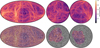 |
Fig. E.1 Mollweide (left) and orthographic (right) projections of one synthetic filamentary model with misalignment around the poles. In colors in the top, we show the total intensity model in normalized units, while in the bottom overlaid drapery patterns also trace the modeled magnetic-field orientation. The orthographic projections are centered around the Galactic poles. In the bottom, we apply the 20% sky mask. The misalignment is uniform and is fixed to 9° in the north and 5° in the south. |
When the B modes are drawn from the H I templates, we find a hint of TdBHI < 0, but this is significant only in the southern hemisphere and only for the spherical RHT. Since the H I templates are constructed entirely independently of dust polarization data, a true signal of TdBHI < 0 would indicate that the H I filamentary morphology displays a chiral asymmetry. This possibility was noted in the conclusion and appendix of Cukierman et al. (2023). A morphological chirality would present an additional contribution to the dust T B. If the morphological contribution is negative, it may partially cancel the contribution from magnetic misalignment. In the absence of a strongly nonzero TdBHI signal, we consider the misalignment effect to be the main contributor to TdBd.
Appendix E Synthetic filamentary all-sky model
This appendix describes the procedure to create all-sky models of non-Gaussian filamentary structures from realizations of synthetic pseudo-random fields, as shown in Fig. E.1. Our approach extends to HEALPix spherical grids the pywavan7 technique developed in Python by Robitaille et al. (2020) for flat-sky models. The key principle of Robitaille et al. (2020) is building a statistical model based on multiplicative random cascades, which are designed to replicate the multi-fractal, hierarchical structure of intermittent features developed in turbulent media such as the ISM. They presented a version of the multiplicative process, where the spatial fluctuations as a function of scale are produced with wavelet transforms of fractional Brownian motion (FBM) realizations. Using directional wavelets, filamentary structures can be produced without changing the general shape of the angular power spectrum of the input FBM realization. The filamentary structures are formed through the product of a large number of random-phase linear waves at different spatial wavelengths (see their Eq. 7). To extend pywavan to the sphere, we made use of the S2WAV Python package8 that computes wavelet transforms on the sphere using JAX (Price & McEwen 2024; Price et al. 2024).9
In the top boxes of Fig. E.1, we show one synthetic all-sky filamentary model obtained at Nside = 128 and FWHM=80' with nine distinct wavelet directions and a FBM input power spectrum of slope −3, typical of H I data at intermediate and high Galactic latitudes (e.g., Miville-Deschênes & Martin 2007; Marchal & Miville-Deschênes 2021). The model is shown both in a Mollweide projection (left) and in an orthographic projection centered around the two Galactic poles (right). In the bottom boxes, including the 20% mask, we show the corresponding magnetic-field orientation that was derived as follows.
We considered the relation between magnetic-field orientations perfectly aligned with density filamentary structures and the respective TEB cross-correlations. In particular, perfect alignment establishes maximal T E correlation without T B correlation (e.g., Zaldarriaga 2001; Planck Collaboration Int. XXXVIII 2016; Bracco et al. 2019a,b; Huffenberger et al. 2020). Given the filamentary sky model used as a proxy of T in arbitrary units, we imposed the corresponding E and B modes as E = T and B = 0, respectively. We converted this TEB system to a Stokes IQU group of maps following standard relations with spherical harmonics (e.g., Bracco et al. 2019a). We used the Python routine called map_teb2iqu, which can be found at the same address written above. The modeled Stokes IQU provided us with the polarization angle and the corresponding magnetic field orientation that perfectly follows the projected morphology of the filamentary sky model. Finally, using a rotation similar to Eq. 3, we introduced two uniform misalignment angles in the two hemispheres, namely, ΔψΝ and ΔψS. This last step mimicked the effect of a large-scale hemispherical misalignment between the filamentary structures, which in this model corresponds to the magnetic field traced by the H I templates, and the total polarization field, which corresponds to the Planck polarization data. Through this synthetic filamentary model we tested the impact of ΔψΝ and Δψδ on the dust polarization power spectra as described in Sect. 5.3.2 and shown in Fig. 12.
All Figures
|
Fig. 1 All-sky masks with sky fractions of 20, 40, 60, and 80% with progressively brighter colors. The gray region along the Galactic plane is not considered in this work. A galactic coordinate grid with steps of 30° in longitude l and latitude b is overlaid with its origin at the Galactic center. |
| In the text | |
|
Fig. 2 Normalized probability distribution functions of Δψ between Planck data at 353 GHz and the H I templates. The value of Δψ is computed for different sky masks at angular and pixel resolutions of 80' and Nside = 128, respectively. The NPDFs are shown for both Galactic hemispheres combined (central panels) and for the southern (left panels) and northern (right panels) hemispheres individually. The corresponding circular-mean values (in black circles) and their standard deviations (in gray diamonds) are shown in the insets at the bottom as a function of the sky mask. The gray shaded area in the middle panels represents the misalignment angle caused by systematic differences between SRoll2 and PR4 data. |
| In the text | |
|
Fig. 3 The NPDFs of Δψ as a function of pd over the 80% mask. The NPDFs were computed in equally sampled bins of pd containing 15633 elements and are represented with bright to dark colors from low to large values of pd, respectively. The central value of each pd bin is plotted on the x axis in the central and bottom panels. The errors on 〈Δψ〉circ are smaller than the symbols. |
| In the text | |
|
Fig. 4 The NPDFs of Δψ, considering the 20% mask and changing the angular resolution of the maps to ℓFWHM. Left and right panels show the southern and northern hemispheres, respectively. The central panel shows them together. More small-scale information is included as ℓFWHM increases. |
| In the text | |
|
Fig. 5 Same as for Fig. 4 but filtering out the large angular scales up to ℓmin. Large-scale information is removed at ℓ < ℓmin as ℓmin increases. |
| In the text | |
|
Fig. 6 Sketch of the toy model showing the LB and the mean magnetic field in the solar neighborhood from the north pole to the Galactic plane (GP, top) and across the GP (bottom). Dark colors correspond to structures of CNM, light colors to the WNM, cyan lines to magnetic-field lines in the CNM, and purple lines to the magnetic-field lines of the WNM. The Sun position in the LB is represented by a red-white circle. An inset in the top panel shows the angle δli between the LB/CNM field and the mean/WNM magnetic field. |
| In the text | |
|
Fig. 7 Modeled misalignment angle between the LB magnetic field and the total one as a function of fL. Hatches show the misalignment in each Galactic hemisphere separately. As an example, the intrinsic misalignment angle δli is ±12° in the southern and northern hemisphere, respectively. The histograms were computed in the 20% mask. In light gray, the cases for both hemispheres with δli = +12° are shown. |
| In the text | |
|
Fig. 8 Dependence of the observed misalignment angle with fL and |δli| in the toy model. Black contours show levels of misalignment angle similar to what was measured in the Planck data. |
| In the text | |
|
Fig. 9 Misalignment angle between polarization data (rotated by 90°) and starlight polarization measurements as a function of the stellar distance for Planck data at 353 GHz (top-left panel), H I polarization templates (top-central panel), and Planck data at 30 GHz (top-right panel). The misalignment is shown in green and pink for the northern and southern he mispheres, respectively. The misalignment peaks at the edge of the LB in cyan. With the same color scheme, the bottom panels show the average normalized kurtosis of the corresponding Δψ distributions. The uncertainty is the standard deviation between the two versions of each dataset. The gray shaded area represents the standard deviation of the average kurtosis of a normal distribution in the case of low-number statistics, as for the number of stars per distance bin (approximately 20). |
| In the text | |
|
Fig. 10 Planck Τ Β power spectra in the northern and southern Galactic hemispheres. Power spectra were computed in the 20% mask with both SRoll2 and PR4 maps. Units are in |
| In the text | |
|
Fig. 11 Planck T B power spectra from both Galactic hemispheres with the 20% mask before and after de-rotation, using SRoll2 for the dust maps and two different H I templates. The de-rotation was computed at ℓref = 20. Units are |
| In the text | |
|
Fig. 12 Modeled T B power spectra as a function of the misalignment angles ΔψN and ΔψS in the north and south Galactic hemispheres, respectively. Power spectra were computed with the 20% mask. |
| In the text | |
|
Fig. A.1 Effect of the angle rotation on the Planck Stokes parameters using Eq. 3. The original data at FWHM=80' are shown in the left column and the maps rotated with respect to ℓref = 20 in the right column. The Stokes parameters are shown in the top and central panels with the same color bar displayed on the left, while polarized intensities are shown in the bottom panels in the background of the drapery patterns tracing the magnetic-field orientation obtained through LIC. The 80% sky mask is applied (see Fig. 1). |
| In the text | |
|
Fig. B.1 Same as for Fig. 4 but considering Planck data at 217 GHz as a test of the robustness of the results for 353 GHz. A similar misalignment as at 353 GHz is also found at 217 GHz. |
| In the text | |
|
Fig. B.2 Same as for Fig. 4 but considering Planck data at 30 GHz, which is dominated by synchrotron radiation rather than dust emission. A stronger misalignment than at 353 GHz is found at 30 GHz, where synchrotron polarization is traced. |
| In the text | |
|
Fig. C.1 Orthographie projection around the northern (left) and southern (right) Galactic poles of the hit map of stars after reprojecting the measurements on a HEALPix grid at Nside = 128. A galactic coordinate grid is overlaid. |
| In the text | |
|
Fig. D.1 Estimates of Τ Β cross spectra for dust and Η I filaments in the two Galactic hemispheres with the 20% mask. This is a comparison between the various spectra depending on the given Planck dataset (left, TdB353) and Η I template (right, TdBHI). To be able to compare all of these quantities, which have different physical units, we have normalized each spectrum to the mean of its absolute values. |
| In the text | |
|
Fig. E.1 Mollweide (left) and orthographic (right) projections of one synthetic filamentary model with misalignment around the poles. In colors in the top, we show the total intensity model in normalized units, while in the bottom overlaid drapery patterns also trace the modeled magnetic-field orientation. The orthographic projections are centered around the Galactic poles. In the bottom, we apply the 20% sky mask. The misalignment is uniform and is fixed to 9° in the north and 5° in the south. |
| In the text | |
Current usage metrics show cumulative count of Article Views (full-text article views including HTML views, PDF and ePub downloads, according to the available data) and Abstracts Views on Vision4Press platform.
Data correspond to usage on the plateform after 2015. The current usage metrics is available 48-96 hours after online publication and is updated daily on week days.
Initial download of the metrics may take a while.