


| Issue |
A&A
Volume 711, July 2026
|
|
|---|---|---|
| Article Number | A213 | |
| Number of page(s) | 21 | |
| Section | Cosmology (including clusters of galaxies) | |
| DOI | https://doi.org/10.1051/0004-6361/202558537 | |
| Published online | 16 July 2026 | |
CHEX-MATE: Are we getting cluster thermodynamics right?
1
Department of Astronomy, University of Geneva, Ch. d’Ecogia 16, CH-1290 Versoix, Switzerland
2
INAF – Osservatorio Astronomico di Trieste, Via Tiepolo 11, I-34131 Trieste, Italy
3
Department of Physics, University of Michigan, Ann Arbor, MI 48109, USA
4
Jodrell Bank Centre for Astrophysics, Department of Physics and Astronomy, The University of Manchester, Oxford Road, Manchester M13 9PL, UK
5
Excellence Cluster ORIGINS, Boltzmannstr. 2, D-85748 Garching bei München, Germany
6
Universitäts-Sternwarte, Fakultät für Physik, Ludwig-Maximilians-Universität München, Scheinerstr.1, 81679 München, Germany
7
Max-Planck-Institut für Astrophysik, Karl-Schwarzschildstr. 1, 85741 Garching bei München, Germany
8
IFPU, Institute for Fundamental Physics of the Universe, Via Beirut 2, I-34014 Trieste, Italy
9
INAF, Osservatorio di Astrofisica e Scienza dello Spazio, Via Piero Gobetti 93/3, I-40129 Bologna, Italy
10
INFN, Sezione di Bologna, Viale Berti Pichat 6/2, I-40127 Bologna, Italy
11
Université Paris-Saclay, Université Paris Cité, CEA, CNRS, AIM de Paris-Saclay, 91191 Gif-sur-Yvette, France
12
IRAP, CNRS, Université de Toulouse, CNES, Toulouse, France
13
INAF, Istituto di Astrofisica Spaziale e Fisica Cosmica di Milano, Via A. Corti 12, 20133 Milano, Italy
14
Dipartimento di Fisica, Sapienza Università di Roma, Piazzale Aldo Moro 5, I-000185 Rome, Italy
15
Department of Physics, Informatics and Mathematics, University of Modena and Reggio Emilia, 41125 Modena, Italy
16
Center for Astrophysics | Harvard & Smithsonian, 60 Garden Street, Cambridge, MA 02138, USA
17
Dipartimento di Fisica, Università di Roma ‘Tor Vergata’, Via della Ricerca Scientifica 1, I-00133 Roma, Italy
18
INFN, Sezione di Roma ‘Tor Vergata’, Via della Ricerca Scientifica, 1, 00133 Roma, Italy
19
California Institute of Technology, 1200 E. California Blvd., Pasadena, CA 91125, USA
20
Departamento de Física Teórica M-8, Universidad Autónoma de Madrid, Cantoblanco, E-28049 Madrid, Spain
21
Centro de Investigación Avanzada en Física Fundamental (CIAFF), Universidad Autónoma de Madrid, E-28049 Madrid, Spain
★ Corresponding author: This email address is being protected from spambots. You need JavaScript enabled to view it.
Received:
12
December
2025
Accepted:
19
June
2026
Abstract
Context. Galaxy clusters offer powerful insights into the large-scale structure of the Universe and the physics of baryons in hot states. Their scientific exploitation, however, hinges on our ability to accurately measure key thermodynamic properties.
Aims. In this work we assess the reliability of current analysis techniques in reconstructing these properties, with a particular focus on samples similar to those observed in the Cluster Heritage project with XMM-Newton (CHEX-MATE).
Methods. We developed a suite of dedicated end-to-end simulations of CHEX-MATE-like clusters selected from large-scale hydrodynamical simulations and processed through a newly developed realistic XMM-Newton simulator. We applied a full X-ray data analysis pipeline that includes imaging, spectral fitting, and profile reconstruction to the mock datasets.
Results. The gas density profiles can be robustly recovered across a wide radial range when using azimuthal mean surface brightness profiles. Our reconstruction techniques are able to reproduce the intrinsic density profile with the correct scatter, with deviations of at most 10% between 0.1 and 1 × R500c. The gas mass is reconstructed with better than 1% accuracy. The accurate measurement of temperature profiles is more challenging and possibly subject to biases, particularly in the presence of azimuthal variations and multi-temperature gas along the line of sight, which dominate over projection effects.
Conclusions. Our results highlight the need for caution when interpreting cluster temperature measurements and underscore the value of tailored mock observations for understanding observational systematics. These findings also suggest that biases in X-ray temperature measurements alter the interpretation of the thermodynamical state of the intra-cluster medium, an outlook particularly relevant in light of recent low-velocity measurements from the XRISM mission.
Key words: methods: data analysis / surveys / galaxies: clusters: intracluster medium / large-scale structure of Universe / X-rays: galaxies: clusters
© The Authors 2026
 Open Access article, published by EDP Sciences, under the terms of the Creative Commons Attribution License (https://creativecommons.org/licenses/by/4.0), which permits unrestricted use, distribution, and reproduction in any medium, provided the original work is properly cited.
This article is published in open access under the Subscribe to Open model. This email address is being protected from spambots. You need JavaScript enabled to view it. to support open access publication.
1. Introduction
Clusters of galaxies are the end point of the structure formation process throughout the history of the Universe and are located in the nodes of the cosmic web (Mo & White 2002; Springel 2005). They encode precious cosmological information about dark matter, which drives the shaping of the large-scale structure of the Universe, and dark energy, which drives its accelerated expansion at late times (Allen et al. 2004; Kravtsov & Borgani 2012; Clerc & Finoguenov 2022; Ghirardini et al. 2024; Lesci et al. 2025). Massive galaxy clusters benefit from high signal-to-noise ratio observations at various wavelengths. In the optical band they are seen as a collection of their galaxy members (Rykoff et al. 2014; Abbott et al. 2020). However, only about 1% of their total mass resides in the galaxy population. About 90% is in the form of dark matter, whose gravitational effect appears as peaks in weak lensing convergence maps (Miyazaki et al. 2018). Finally, the majority of baryons are located in the hot gas that constitutes the intra-cluster medium (ICM), heated by the process of gravitational collapse to high temperatures of around 108 K. This allows clusters to be detected in the millimetre band via the Sunyaev-Zeldovich (SZ) effect (Staniszewski et al. 2009; Planck Collaboration XXVII 2016) and in X-rays thanks to direct emission via thermal bremsstrahlung (Böhringer et al. 2004; Pratt et al. 2019). SZ surveys such as those conducted by the Atacama Cosmology Telescope (ACT; Hilton et al. 2021), the South Pole Telescope (SPT; Bleem et al. 2020), and Planck (Planck Collaboration XXVII 2016) are sensitive to most massive clusters up to high redshifts. X-ray surveys from ROSAT (Böhringer et al. 2004), XMM-XXL (Pierre et al. 2016), and eROSITA (Predehl et al. 2021; Bulbul et al. 2024) are better suited to detecting the low-mass cluster population, but their sensitivity quickly drops at high redshifts. The combination of multi-wavelength data is essential to obtain a clear view of galaxy clusters in the Universe (e.g. Beauchesne et al. 2024).
The Cluster HEritage project with XMM-Newton: Mass Assembly and Thermodynamics at the Endpoint of structure formation (CHEX-MATE1; CHEX-MATE Collaboration 2021) was designed to follow up on a sample of 118 galaxy clusters selected from Planck with X-ray observations using XMM-Newton. The programme covers three mega-seconds, with a median exposure time of 40 ks per object. The goal is to study the final products of structure formation, focusing on lower-mass clusters at low redshifts (Tier-1: 0.05 < z < 0.2, 2 × 10¹⁴< M500c/M⊙ < 9 × 10¹⁴) and the most massive clusters in the Universe (Tier-2: z < 0.6, M500c > 7.25 × 10¹⁴ M⊙). CHEX-MATE aims to combine the deep XMM observations with archival and follow-up lensing and SZ data to tackle some open questions in cluster science, such as regarding mass calibration, different selection processes, and the evolution of cluster properties throughout cosmic time. The CHEX-MATE collaboration has already produced several results relevant to this work. Campitiello et al. (2022) derived a dynamical-state indicator from X-ray morphological parameters, finding that CHEX-MATE clusters are generally more disturbed than X-ray–selected samples. Bartalucci et al. (2023) show that surface-brightness profiles exhibit a large diversity in the cores but converge with minimal scatter at 0.4–0.8 R500c. Temperature profiles for a representative subsample were presented by Rossetti et al. (2024), who demonstrated the potential for statistical studies once the full sample is analysed. A pilot study of entropy profiles by Riva et al. (2024) revealed correlations between the core entropy and dynamical state as well as deviations from self-similar scaling. The CHEX-MATE data quality also enables advanced mass-modelling approaches – Kim et al. (2024) combined XMM-Newton and Planck data to obtain 3D elliptical models (Kim et al. 2024; Chappuis et al. 2025) – and determinations based on galaxy dynamics (Sereno et al. 2025). Finally, Muñoz-Echeverría et al. (2025) introduced a joint fitting of universal pressure profiles and cluster masses to break their degeneracy, a method well suited to CHEX-MATE.
Rigorous validation of the X-ray analysis pipeline further strengthens the accuracy and precision of the recovered observables and the cluster properties inferred from them. The need for tools capable of producing realistic mock X-ray observations from hydrodynamical simulations emerged as a crucial step towards bridging the gap between theory and observation. Early works (Evrard et al. 1996; Mathiesen & Evrard 2001) emphasised that meaningful comparisons with X-ray data require simulated quantities that incorporate projection and instrumental effects, rather than purely theoretical profiles. This concept was operationally realised with the development of dedicated X-ray map simulators, such as X-MAS (Gardini et al. 2004), which for the first time reproduced the full observing process – including telescope response, background noise, and photon statistics – yielding realistic event files for instruments such as Chandra and XMM-Newton. Subsequent studies (e.g. Rasia et al. 2006; Nagai et al. 2007; Rasia et al. 2008; Biffi et al. 2012) demonstrated that such simulated observations are essential to quantify observational biases, test data analysis pipelines, and ensure that theoretical predictions and observed cluster properties are compared on consistent grounds. These developments have firmly established X-ray map simulators as a cornerstone in the modern analysis of the ICM. The literature is rich with such examples, especially in the X-ray band (see also Lau et al. 2009; Battaglia et al. 2013; Nelson et al. 2014; Rasia et al. 2015; Biffi et al. 2016), but also in combination with other probes like lensing (Meneghetti et al. 2010, 2011; Rasia et al. 2012; Euclid Collaboration: Giocoli et al. 2024; Giocoli et al. 2025) and the SZ effect (Gupta et al. 2017; Gianfagna et al. 2021; Wicker et al. 2023). Most such studies focus on recovering intrinsic properties such as halo mass and provide estimates of the hydrostatic mass bias ranging between 10 and 30% (Gianfagna et al. 2023; Jennings & Davé 2023; Muñoz-Echeverría et al. 2024), with the bias increasing with cluster mass (Braspenning et al. 2025). Other works suggest that part of the mass bias is encoded in X-ray temperature measurements (Henson et al. 2017; Pearce et al. 2020; Barnes et al. 2021). They assume various levels of complexity concerning how realistic the X-ray mock is, starting from the simplest approach of analysing the hot gas particles in hydrodynamical simulations with dark matter and baryons.
Following the examples of Rasia et al. (2008) and Biffi et al. (2013), our goal is to take one step further by selecting twin CHEX-MATE samples from three different hydrodynamical simulations: The Three Hundred (The300 hereafter) project (Cui et al. 2018), Magneticum (Dolag 2015), and MACSIS (Barnes et al. 2017). We generated realistic end-to-end XMM-like mock observations and analysed them with standard tools and pipelines widely used in the X-ray community. The high resolution of the simulations, together with realistic X-ray processing, enabled a robust comparison between recovered and input thermodynamic profiles. This is essential for assessing whether our models can accurately reproduce X-ray measurements and recover intrinsic cluster properties without bias. We find that the gas density and gas mass reconstruction is robust within a few percent. The reconstruction of the X-ray temperature is in agreement with expectations, but its direct link to mass is not straightforward: the results depend on the hydrodynamical simulation, and temperature biases propagate to pressure and entropy at the 10 − 20% level. The focus of this work is not on comparing the physical differences between simulations but rather on using them as controlled laboratories to assess the performance of X-ray analysis techniques. By applying the same analysis pipeline to synthetic observations and comparing the results to the known input quantities, we isolate biases arising from observational procedures and modelling assumptions.
Radial profiles were normalised to the true cluster radius, providing a consistent scale for input-output comparison, while centring and reconstruction were carried out independently through the X-ray analysis. A detailed investigation of the impact on mass and radius estimates is deferred to future work. The best-fit results are always median values accompanied by their 16th–84th percentile points. This article is organised as follows. In Sect. 2 we present the simulations used in this work. In Sect. 3 we explain the generation of the mock XMM-Newton data. In Sect. 4 we describe the X-ray analysis of the mock data. We present our results on the X-ray observables in Sect. 5. We further discuss them and summarise our work in Sect. 6.
2. Hydrodynamical simulations
We briefly describe the hydrodynamical simulations used in this work, but refer to their presentation papers for a more in depth description. A summary is reported in Table 1.
Cosmological and numerical parameters describing the The300, Magneticum, and MACSIS simulations.
2.1. The300
The300 simulations consists of 324 regions centred on large galaxy clusters simulated with baryons including processes related to galaxy formation and evolution, gas cooling, supernova and active galactic nucleus (AGN) feedback (Cui et al. 2018). The clusters have been initially identified by the Rockstar halo finder (Behroozi et al. 2013) in the 1 h−1 Gpc dark-matter-only MDPL2 box (Klypin et al. 2016)2. The dark matter haloes are selected to have virial mass larger than 8 × 10¹⁴ h−1 M⊙3.
In the re-simulation process, the dark matter particles within each of the selected region of radius ∼15 h−1 Mpc, are split into dark matter and gas, according to the cosmological baryon fraction and with an initial gas mass resolution of 2.36 × 10⁸ h−1 M⊙. The re-simulation was performed with GADGET-X (Beck et al. 2016) using smooth-particle hydrodynamics (SPH) and haloes and sub-haloes were identified by the AMIGA Halo Finder (AHF; Knollmann & Knebe 2009), which accounts for the baryonic components in the halo finding process. The baryonic physics includes models for gas cooling (Wiersma et al. 2009), stellar evolution (Tornatore et al. 2007), stellar feedback (Springel & Hernquist 2003), black hole growth and AGN feedback (Steinborn et al. 2015). Cosmological parameters are from Planck Collaboration XIII (2016). The300 project reproduces the baryon fraction and scaling relations of local galaxy clusters down to 1013 M⊙. Recent work from Rasia et al. (2025) highlighted the importance of properly modelling the hot gas fraction in galaxy clusters. In particular, The300 compares well with CHEX-MATE in terms of emission measure profiles (Bartalucci et al. 2023), temperature profiles and their inhomogeneities (Rossetti et al. 2024; Lovisari et al. 2024), and gas pressure and entropy for the most massive systems (Riva et al. 2024).
2.2. Magneticum
The Magneticum suite4 is a collection of full cosmological hydrodynamical simulations (Dolag et al. 2025). They are performed with the P-GADGET3 code (Springel 2005). They include baryonic process such as AGN feedback (Fabjan et al. 2010), star formation, supernovae explosions, galactic winds (Springel & Hernquist 2003), gas cooling (Wiersma et al. 2009), and enrichment (Tornatore et al. 2007). The cosmological parameters are taken from the WMAP results (Komatsu et al. 2011). In particular, we selected galaxy clusters from the Box2 and Box2b in their high resolution (hr) version, respectively with sizes of 352 and 640 Mpc h−1, and dark-matter and gas particle masses of 6.9 × 10⁸ M⊙ h−1 and 1.4 × 10⁸ M⊙ h−1. Box2b was run until z = 0.2; therefore, all the clusters at lower redshifts were selected from Box2. Galaxies and clusters were identified using a friends-of-friends algorithm combined with Subfind (Dolag et al. 2009).
Magneticum successfully reproduces the AGN luminosity function (Hirschmann et al. 2014), morphological properties of clusters (Teklu et al. 2015; Remus et al. 2017; Gupta et al. 2017), thermodynamical profiles and features of galaxy groups (Bahar et al. 2024; Popesso et al. 2025). It was exploited to study the hydrostatic mass bias and recovery of X-ray observables in the context of eROSITA (Scheck et al. 2023; ZuHone et al. 2023).
2.3. MACSIS
The MAssive ClusterS and Intercluster Structures (MACSIS; Barnes et al. 2017) dataset is a collection of 390 re-simulated regions carried out with full baryonic physics. The concept is similar to the one presented by The300 project in Sect. 2.1, with an initial selection on a large N-body simulation followed by a re-simulation that includes the baryonic components. The parent simulation is a dark-matter-only cube of 3.2 Gpc, run with GADGET3 (Springel 2005). The cosmological parameters are taken from Planck Collaboration XVI (2014). The dark matter particle mass is 5.43 × 10¹⁰ h−1 M⊙. The MACSIS sample was selected from all haloes more massive than 1015 M⊙ at z = 0, identified by a friend-of-friend algorithm. These haloes were grouped into mass bins of 0.2 dex. If a bin contained fewer than 100 haloes, all of them were selected; otherwise, the bin was refined to 0.02 dex, from which 10 objects were randomly selected.
These haloes were re-simulated with full baryonic physics following the prescriptions from BAHAMAS (McCarthy et al. 2017). Similarly to The300 and Magneticum, the baryonic model includes radiative cooling from different elements (Wiersma et al. 2009), star formation and feedback (Schaye & Dalla Vecchia 2008), as well as black hole seeding, growth, and feedback (Booth & Schaye 2009). The hot gas profiles from MACSIS show good agreement with observational data (Barnes et al. 2017; Riva et al. 2024).
2.4. Simulated cluster sample
We selected clusters by picking a twin for each real CHEX-MATE cluster with the closest possible mass in the various redshift snapshots. For The300 and MACSIS, a 20% hydrostatic mass bias is applied when matching observed clusters to simulated analogues. Although this introduces heterogeneous assumptions on bHE, it has the advantage that our analogue sample spans the full range from no bias to 20%. As a result, the reconstruction tests naturally assess the robustness of our methods across the plausible range of hydrostatic mass biases, rather than relying on a single fixed value. The hydrostatic bias parameter bHE is treated here as a nuisance parameter. Since its true value is not known a priori, we adopted representative values motivated by the literature to test the robustness of our results to this assumption. Our goal is not to constrain bHE, but to verify that the recovery of thermodynamic quantities is not sensitive to reasonable variations in this parameter. As explained in Sect. 1, CHEX-MATE is split into Tier 1 and Tier 2 clusters. Because of its construction containing exclusively massive systems, MACSIS is associated only with Tier 2 objects. Instead, for The300 and Magneticum we included matched samples for both Tier 1 and Tier 2. Very nearby systems filling the full XMM-Newton field of view (FoV) were excluded from the analysis. Visual inspection of the simulated images showed that, for these objects, cluster emission remains evident up to the edge of the image, precluding a reliable determination of the local background and a profile reconstruction out to R500c within a single pointing. While such clusters are observed using mosaics in CHEX-MATE, reproducing these observing strategies is beyond the scope of the present work. This criterion removes only a small number of systems (two MACSIS clusters and three The300 clusters) and does not affect the main conclusions. Figure 1 shows the distribution of CHEX-MATE clusters (in red) in the mass-redshift space, together with the twin-selected systems from The300 (in blue), Magneticum (in orange), and MACSIS (in green).
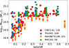 |
Fig. 1. Mass and redshift distribution of the CHEX-MATE clusters compared to the twin-selected systems from The300, Magneticum, and MACSIS. The CHEX-MATE masses include the hydrostatic mass bias of 0.2. |
Because the snapshots of the simulations are saved at different redshifts, the matching with the redshifts of real CHEX-MATE objects may be more or less precise, especially at high redshifts, where the snapshot of the Magneticum Box2b are sparse; the systems around redshifts of 0.6 are matched to the snapshot at 0.67. This is not a limitation for our goals, as we did not aim to study the properties of individual clusters but focused on a comparison at the population level to input properties using a global sample that is representative of CHEX-MATE. The adopted selection provides a manageable sample size while remaining representative of the parameter space explored by CHEX-MATE. In addition, the selected samples provide the basis for future work aimed at direct comparisons between CHEX-MATE observations and realistic mock observations drawn from hydrodynamical simulations. The purpose of the selected sample is not to provide a statistically representative description of the global cluster population, but rather to test the ability of the forward-modelling and analysis pipeline to recover thermodynamic properties from realistic mock X-ray observations.
3. Mock generation
We used the individual gas particles in the simulations to construct an emissivity model projected along the line of sight in a 30′×30′ FoV. We folded the model through the response of XMM-Newton and generated mock events assuming a clean 25 ks exposure time. We then analysed the mock X-ray data by extracting surface brightness and temperature profiles and applying a deprojection technique (details in Sect. 4).
3.1. Input data
To generate the X-ray emission from each gas particles, we used the first unit of the code X-ray Map Simulator described in Gardini et al. (2004) with some modification as follows. The gas particles are selected within a temperature range of [0.3 − 40] keV and with a gas density below the star formation threshold to guarantee that multi-phase particles are not included. We stress that this does not mean that emission below 0.3 keV is ignored, because gas elements at different temperatures also shine in the softest X-ray band. The FoV covers 30 × 30 arcmin2 and it is sampled with a grid of 512 × 512 pixels. We created 495 narrow energy channels, linearly spaced between 0.1 and 10 keV, and summed and projected along one random axis the emissivity of the individual particles. Specifically, the projected spectra assume thermal emission from a collisionally ionised diffuse gas with a fixed metallicity of 0.3 Z⊙ (Asplund et al. 2009) and is corrected by an absorption term assuming a hydrogen column density of 5 × 1020 cm−2 (i.e. in Xspec: phabs(apec)). The final projected flux is stored in a data cube of size 512 × 512 × 495. Effectively, this information is similar to that of an ideal integral field unit (IFU), where for each pixel we have access to the input global spectrum.
3.2. XMM simulation
We used the data cube obtained in the previous section as an input to the xmm_simulator5 software to generate realistic XMM-Newton simulations. We built a 2D model image for each energy channel. We computed the effective area on the pixel grid, accounting for the detector quantum efficiency, filter transmission, CCD gaps, and the telescope vignetting by combining each component in the XMM current calibration files (CCF)6. We also included the non-X-ray background by loading filter wheel closed data from the CCF for each camera. Its intensity is constant on the detector surface, i.e. there are no soft protons. We modelled the sky background including contributions from the foreground, with the local hot bubble (an unabsorbed apec model with a temperature of 0.11 keV), the galactic halo (an absorbed Phabs(apec) model with a temperature of 0.22 keV), and the cosmic X-ray background (CXB) with contribution from the faint, undetected AGN (an absorbed power law Phabs(Power) with a spectral index Γ = 1.46). Finally, we included the emission of AGNs by randomly generating their position within the FoV. This means that no AGN clustering is present, but this is negligible given the size of the XMM FoV, and 1D cluster profile studies are not affected. The fluxes are drawn from the logN-logS distribution of Lehmer et al. (2012). The AGN spectral model is an absorbed power law with column density randomly drawn in the range [1020 − 1023.5] cm−2 and a slope drawn from a Gaussian distribution with mean of 1.9 and variance 0.2 (Ueda et al. 2014).
For each energy channel, the total model image with the source, sky background, and AGN was recast into XMM pixels, convolved with the point spread function (PSF) and the response matrix file. Individual events were generated as a Poisson realisation of the total model, including a separate particle background photon list that was merged with the event file. We generated mock EPIC events with an exposure time of 25 ks, which is representative for the CHEX-MATE observations.
4. X-ray analysis
We reduced the mock data with dedicated software to analyse XMM-Newton data XMM_SAS version 21.07, routines from pyproffit8 (Eckert et al. 2020) and hydromass9 (Eckert et al. 2022). We note that this pipeline is not identical to that used for CHEX-MATE, although they share most of the underlying methodology. We ignored 4 (3, 3) clusters in The300 (Magneticum, MACSIS) with complex shapes due to recent major mergers, where assumptions such as spherical symmetry fail.
4.1. Extraction of images and spectra
First we created images in the 0.7–1.2 keV band by combining the individual detectors, MOS1, MOS2, and PN, into a single EPIC XMM image. We also generated a single exposure map by summing together individual exposure maps, while multiplying the one relative to the PN detector by 3.42, that is, the ratio of the PN to MOS effective area in this energy band. We used the ewavelet task to run a wavelet source detection algorithm on the mock images. This allowed us to identify individual point sources to be masked during the X-ray analysis. We carefully visually inspected each region file obtained by the source detection process. The central detection relative to the simulated cluster obviously needed to be removed. This is straightforward. However, sometimes the algorithm splits the clusters into multiple fake sources, or does not include the tails of the point source emission within the aperture corresponding to AGN detections. We manually modified each region mask to include the most amount of clean emission from the cluster, while minimising the impact of sub-haloes, nearby systems, and AGN leakage to the best of our abilities. This step does not involve any prior knowledge from the simulation and the mock is treated exactly as a real observation. From the simulation perspective, we could identify whether masked detections correspond to injected AGNs or to non-AGN features, such as substructure or background fluctuations. Across the three simulations we find no significant variation in the substructure fraction: approximately 75% of masked sources are bona fide AGNs with 5 × 10⁻¹⁴ erg/s/cm2.
Secondly, we prepared the regions to extract spectra to measure the radial temperature profile. By default, the radial profiles consist of one inner bin from 0 to 0.04 × R500c, in addition to 12 more bins spanning from 0.04 to 1.1 × R500c. We extracted the background spectrum in a circular region located between 1.5 and 2.0 × R500c. If the upper boundary overshot the XMM FoV, we manually set it to 15 arcmin. We carefully inspected each region automatically generated by our pipeline and modified it if needed. In some cases the background region was too large and fell outside the FoV. In other cases it ended up including a filament or part of a secondary nearby structure. For such cases, we extracted the background spectrum in one of the FoV corners using a circular aperture of about 3 arcminutes according to the needs of each specific case. An example of the end result of the whole procedure is shown in Fig. 2.
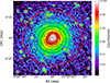 |
Fig. 2. Example of a simulated XMM-Newton EPIC image for one cluster. The black lines denote the regions used for spectral extraction to measure its temperature profile. The red circle denotes R500c. |
Finally, we fitted each spectrum using the X-COP pipeline (Ghirardini et al. 2019). The global model accounts for a high energy particle background (a broken power law with several Gaussian lines), the sky background including the CXB (an absorbed power law with photon index of 1.46), the Galactic halo (an absorbed apec model with temperature between 0.15 and 0.6 keV), and the local hot bubble (an unabsorbed apec model with temperature of 0.11 keV). We turned off the soft protons (an additional broken power law), since we did not simulate them. The source model is an absorbed apec model with temperature, normalisation, and abundance free to vary. In the X-COP pipeline, background modelling is improved by simultaneously fitting the background extracted from the XMM field with ROSAT All-Sky Survey (RASS) background data, which are automatically retrieved in the region surrounding the source. To replicate this approach in our simulations, we generated synthetic X-ray background spectra composed of the same physical components used in the pipeline, i.e. the CXB, Galactic halo emission, and the local hot bubble. Each component is simulated with the same temperatures, abundances, and normalisations adopted in the xmm_simulator, and convolved with the ROSAT Position Sensitive Proportional Counter (PSPC) response files. The simulated background spectrum is normalised to the extraction area, which by default corresponds to a circular annulus between 60 and 90 arcminutes from the source centre. To remain consistent with the simulation setup, we omitted the cross-calibration correction factor between the ROSAT PSPC and the XMM-Newton EPIC camera that is otherwise applied in the X-COP pipeline. This procedure ensures a consistent background treatment and yields more robust temperature measurements, particularly in the outer radial bins where the signal is background-dominated. We used X-SPEC (v12.13.1 Arnaud 1996) with C-stat (Cash 1979). We refer the reader to Ghirardini et al. (2019) for additional details on the X-COP pipeline.
4.2. Measurement of X-ray properties
We extracted surface brightness profiles from the EPIC mosaic and from its Voronoi-binned image. We refer to them as the mean and median profiles, respectively. The median profile is derived from the Voronoi-tessellated map, where each adaptive bin is assigned the median value of its constituent pixels before computing the radial profile. The mean profile is extracted directly from the original image by averaging the native pixels in each radial annulus, without any adaptive binning. Thus, the terms ‘median’ and ‘mean’ describe the construction of the underlying maps rather than different statistics applied to the same pixel set. We used the tessellation scheme from Diehl & Statler (2006), grouping the count maps into cells containing 25 events each to create the final Voronoi image. We then used this image to generate azimuthal median profiles. This alleviated the issue of dense regions biasing the recovered gas density high due to its squared relation to emissivity. The surface brightness profile was modelled as a collection of Kings functions, which enabled the 2D projected profile to be computed analytically. In particular, the cluster X-ray emissivity follows 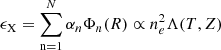 , where
 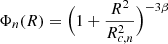 and Λ(T, Z) is the cooling function, which depends on temperature and metallicity (Sutherland & Dopita 1993). The model is convolved with the PSF, and superimposed to a constant background profile that is estimated by computing a count rate value from the spectral model of the background obtained in Sect. 4.1. We refer the reader to Eckert et al. (2020) for a detailed description of the surface brightness measurement and modelling.
We then modelled the gas and mass profiles under the assumptions of hydrostatic equilibrium and spherical symmetry, which allowed us to link the gas pressure to the total mass. Gas density, temperature, and thermal pressure are related by the ideal gas equation of state. We denote the gas mass density with ρgas and the gas electron number density with ne. The formalism reads
 (1)
(1)
One can then model the data using Eq. (1) from different points of view, although the observables in question are always gas density and temperature:
-
(i)
Assuming a mass profile using a Navarro-Frenk-White model (NFW; Navarro et al. 1996): given the definition of a mass model, it is possible to derive pressure by integrating the hydrostatic equilibrium equation (first line in Eq. (1)). Temperature is inferred using the ideal gas equation of state (second line in Eq. (1)), while gas density is related to the surface brightness via the cooling function.
-
(ii)
Modelling the temperature profile with a non-parametric (NP) model: a linear combination of log-normal functions is used to describe the 3D temperature profile. It is then projected along the line of sight and fitted to the measurement.
-
(iii)
Modelling the pressure profile with a forward model (FM): a generalised NFW is used to describe the pressure profile, which allows its gradient and the mass profile to be computed analytically. It is linked to temperature (the observable) through the ideal gas law (second line in Eq. (1)).
The model is fitted to total (gas and dark matter) mass. We refer the reader to Eckert et al. (2022) for full details on the modelling. Finally, one can derive the entropy from the 3D temperature and density profiles as 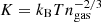 .
.
5. Results
In this section we compare the profiles obtained from the analysis in Sect. 4 to the input quantities measured directly using the properties of the gas particles in the hydrodynamical simulations. We used the three simulations as independent realisations of cluster populations to test the robustness of the recovery of thermodynamic properties. Differences between simulations are therefore interpreted in terms of variations in physical conditions, rather than as the primary focus of the analysis.
5.1. Gas density profiles
Gas density is the most fundamental thermodynamic quantity accessible in X-rays, as the surface brightness directly probes ne2 and is therefore less model-dependent than temperature. It is key to infer cluster properties such as gas mass, pressure, and entropy, and is essential for comparisons with SZ and lensing. We studied the density reconstruction on a population level. We compared input-output profiles on a per-cluster basis, i.e. we always show the distribution of individual-cluster ratios, rather than the ratio of the median reconstructed and true profiles. The input profiles are computed with hot gas particles ≥3 keV. This holds for all results across the article.
Figure 3 shows the recovered median and true density profiles for the three simulation suites. Overall, the agreement is good: discrepancies are limited to the innermost 0.1 R500c in Magneticum, and remain within the scatter of the measurements. The300 and MACSIS exhibit similar core shapes and normalisations, while Magneticum shows flatter and lower-density cores, due to the lower typical masses and the distinct baryonic-physics implementation (see Rasia et al. 2025). A simple beta model10 fit is close to the expectation β = 2/3, but the flatter profile in Magneticum causes a larger core radius in the best fit. We performed the fitting with the curve_fit package in scipy (Virtanen et al. 2020). We report the values in Table A.1. The best-fit parameters are always compatible within uncertainties between the input and recovered profiles. A single β-model cannot capture the full complexity of all clusters, so the fitted parameters should be regarded as descriptive summaries rather than ground truths, used to illustrate the flexibility of the reconstruction. Small differences in the core are likely due to mis-centring (see Appendix G): the observed profiles are computed from using the peak of the X-ray emission in the XMM mocks, while the input profiles are computed from the position of the most bound particle in each cluster.
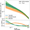 |
Fig. 3. Gas density profiles in our simulations. Top: Comparison between the measured (solid lines and shaded areas) and true (dashed lines) gas density profiles in different simulations (in various colours), using the NFW reconstruction. Bottom: Intrinsic dispersion in the selected population as a function of radius in units of dex. |
The bottom panel of Fig. 3 shows the intrinsic dispersion σintr of the profiles presented in the top panel (using the selected cluster population in each simulation), in units of dex. It is the average of the upper and lower deviations from the median, i.e. ![Mathematical equation: $ \sigma_{\mathrm{intr}} = \dfrac{1}{2}\left[\log_{10}\left(\dfrac{P_{84}}{P_{50}}\right) + \log_{10}\left(\dfrac{P_{50}}{P_{16}}\right)\right] $](/articles/aa/full_html/2026/07/aa58537-25/aa58537-25-eq5.gif) , where P16, P50, and P84 denote the 16th, 50th, and 84th percentiles of the distribution at fixed radius. Among the simulations, MACSIS exhibits the largest scatter in the core region (within 0.1 × R500c), reaching values up to 0.3 dex, whereas The300 remains below 0.25 across the same range. Magneticum displays the most diverse behaviour at intermediate radii, with a scatter peaking at 0.21 dex around 0.2 × R500c, while The300 and MACSIS are closer to 0.12 dex at this radius. In the outskirts beyond 0.8 × R500c, all simulations converge to a similar relative scatter of about 0.1 dex. Importantly, the true profiles closely track the measured profiles: the reconstructed gas density profiles not only match the true median profiles but also reproduce the true population scatter in the population as a function of radius.
, where P16, P50, and P84 denote the 16th, 50th, and 84th percentiles of the distribution at fixed radius. Among the simulations, MACSIS exhibits the largest scatter in the core region (within 0.1 × R500c), reaching values up to 0.3 dex, whereas The300 remains below 0.25 across the same range. Magneticum displays the most diverse behaviour at intermediate radii, with a scatter peaking at 0.21 dex around 0.2 × R500c, while The300 and MACSIS are closer to 0.12 dex at this radius. In the outskirts beyond 0.8 × R500c, all simulations converge to a similar relative scatter of about 0.1 dex. Importantly, the true profiles closely track the measured profiles: the reconstructed gas density profiles not only match the true median profiles but also reproduce the true population scatter in the population as a function of radius.
We find excellent agreement between different reconstruction methods, with the median profiles from the Voronoi images showing the greatest precision (see Fig. A.2 and the discussion in Appendix A). In Appendix A we also show that the integration of gas density profiles to measure gas masses also recovers the input gas mass accurately with the Voronoi approach to better than 1% precision, while the standard processing tends to overestimate gas mass by about 5%.
5.2. Temperature profiles
Temperature is a fundamental X-ray observable of galaxy clusters. As a quantity obtained directly from spectral fitting, it traces the depth of the gravitational potential and underpins hydrostatic mass estimates. Its radial profile constrains the thermodynamic structure of the ICM and, together with pressure, calibrates the scaling relations used in cluster cosmology. Biases in the recovered temperature arising from multi-temperature structure, projection, or instrumental effects therefore propagate directly into mass estimates and the interpretation of ICM physics.
5.2.1. Temperature weighting schemes
Unlike gas density, for which the true profile is easily defined using the particles, the notion of a true temperature profile is inherently ambiguous: although each gas element has a well-defined internal energy and thus a temperature, any radial profile or integrated quantity requires adopting a weighting scheme. The inferred temperature is sensitive to this choice (Mazzotta et al. 2004; Rasia et al. 2014), especially in the presence of multi-phase gas. Observationally, spectral fitting preferentially weights cooler, denser phases of the ICM with stronger X-ray emission. To reflect these effects in our comparison, we considered two standard definitions. The mass-weighted (MW) temperature follows the assumption that more massive gas elements contribute proportionally more to the thermal energy budget. It is a physically motivated thermodynamic average linked to the gravitational potential and should be the benchmark for comparisons to observations based on combinations to the SZ effect. However, it does not fully capture the complex dependence of X-ray emissivity on both gas density and temperature, particularly in the presence of temperature inhomogeneities or multi-phase structures (Gaspari et al. 2020), also because the typical response of X-ray instruments is higher at soft energies around 2 keV and lower for hotter gas above 3 keV. Instead, the spectroscopic-like (SL) scheme, introduced by Mazzotta et al. (2004) is constructed to emphasise denser, cooler gas phases that dominate the observed X-ray emission in XMM-Newton and Chandra data. It yields robust estimates for high-temperature plasma hotter than about 3 keV, making it particularly suitable for galaxy clusters in the mass range considered here. They are defined as follows:
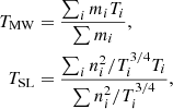 (2)
(2)
where m and n are respectively the mass and the density of each individual gas particle, and the index i identifies each particle within its volume, i.e. a spherical shell in the case of a 3D profile and a cylindrical shell for 2D profiles. In this work, we tested these weighting schemes with a full forward modelling of the XMM observations for the first time.
First we compared the radial profile of the measured temperature obtained by spectral fitting in annuli (TX) to the expected TSL. We focused on TSL here because this is the temperature we expect to measure from X-ray data, as outlined above. Its weighting scheme allowed us to account for the different density and temperature of 3D shells projected along the line of sight as seen by X-ray instruments (Mazzotta et al. 2004). The result is shown in Fig. 4. This is close to one for The300 and Magneticum, but it is underestimated in the cores of MACSIS, within about 0.2 × R500c by at most about 10% (although the one-to-one line is still within the scatter of MACSIS profiles). We ruled out this being due to PSF effects because the median PSF scale of 30 arcsec corresponds to about 0.11 × R500c in MACSIS, compared to about 0.08 (0.105) in The300 (Magneticum). Instead, we find this effect to correlate with cool cores (CCs; see the dashed and dotted lines in Fig. 4). We classified systems based on the ratio between the TSL profile measured at 0.05 and 0.2 R500c
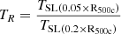 . If TR < 0.8, we classified the system as CC, or as non-cool core (NCC) otherwise. Given this definition, only 8 clusters are classified as CC in The300, for a CC fraction of about 7.5%. This is due to the flat temperature profiles in The300 (see Fig. 5): the median TR is 1.05, while the 16th and 84th percentiles are 0.84 and 1.2. Magneticum shows steeper profiles, with a median TR of 0.75, and 16th–84th percentiles of 0.56 and 1.02. The CC fraction is indeed higher at 62%. MACSIS shows the steepest profiles, with the lowest median TR of 0.70, and 16th–84th percentiles of 0.53 and 0.91. It also yields the highest CC fraction of 76%. We then compared the TX/TSL ratio for CC and NCC subsamples (dashed and dotted lines in Fig. 4). In all cases we find a lower TX/TSL ratio for the CC population across all radii. The difference is most pronounced in MACSIS, where the temperature gradients are large, producing a clear TX/TSL offset: the NCC subsamples resemble The300, but the CC subsamples are underestimated by up to ∼15%. The difference is less clear in The300, with an under-estimation of at most 5% for the CC population, thanks to the flatter profiles. Similarly, MAGNETICUM does not yield a striking difference between CC and NCC subsamples, likely due to the flatter and lower density profiles that also enter the SL weighting scheme (Eq. (2)). Mazzotta et al. (2004) defined the weight of 0.75 in TSL to accommodate a combination of various plasma phases, although some variations are expected: their Fig. 9 shows that the larger the difference between the temperature of two plasma, the larger the deviations in TSL compared to TX. This is particularly relevant for MACSIS: the temperature profiles are steep, so the 2D projection of the core contains plasma phases around 4–5 keV as well as 8–9 keV, where deviations around the 10% level are expected. Finally, Rossetti et al. (2024) show that the CHEX-MATE temperature profiles are in agreement with The300 and do not exhibit the steep profiles that are typical in MACSIS. This suggests that TSL is in an excellent proxy for TX in the real CHEX-MATE sample. For more complex systems and strong CCs, multi-temperature fits are required. In any case, the agreement is excellent also for MACSIS outside of 0.2 × R500c, so that total mass measurements more sensitive to local temperature and temperature gradient around R500c are not affected by the discrepancy in the core. Nonetheless, we verified that the temperature modelling from the observer’s perspective is indeed able to reconstruct the measured temperature profile (see Fig. B.1).
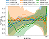 |
Fig. 4. Ratio between the result of the X-ray spectral fitting and the input SL temperature profile. The profiles are also split between CC and NCC according to the ratio between the TSL profile measured at 0.05 and 0.2 R500c (TR). CC (NCC) have a ratio below (above) 0.8. |
In the main panels of Fig. 5 we present the reconstructed 2D temperature profiles from the NFW, NP, and FM models, compared to the true TSL and TMW profiles for each simulation. The profiles were rescaled to T500c adopting the X-COP cluster sample calibration, following Ghirardini et al. (2019, see their Eq. (10)). The smaller panels show output-input ratios: the top rows compare 2D reconstructed temperature to TSL, and the bottom rows show the corresponding ratios for the deprojected 3D profiles. In each panel we also report the median T500c for each sample. We find this to be low for Magneticum at 5.57 keV compared to 6.96 keV for The300 and 8.02 keV for MACSIS. This is expected because the sample from Magneticum has intrinsically less massive systems (Sect. 2.4).
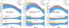 |
Fig. 5. Gas temperature profiles. Each column corresponds to one simulation: The300 (left), Magneticum (centre), and MACSIS (right). The colours denote the three reconstruction methods. The smaller lower panels show the ratio between the reconstructed 2D and deprojected 3D profiles. |
Similarly to gas density, the three simulations show different behaviours also in the temperature profiles. The300 exhibits flat cores with temperatures very close to T500c within 0.3 × R500c, while MACSIS and Magneticum produce clusters with lower temperatures in the core. In particular, MACSIS has strong CCs with temperature being about 30% lower than T500c at 0.05 × R500c. We find evidence that the stronger cooling in MACSIS suppresses the global ICM temperature, in fact, using the T500c normalisation from Ghirardini et al. (2019), the average T(r)/T500c profile in MACSIS remains below unity over the full radial range examined. In comparison, The300 and Magneticum reach (and locally exceed) unity, though with different profile shapes. These trends imply that, at fixed halo mass, MACSIS yields cooler clusters overall – consistent with enhanced cooling efficiency lowering the thermal energy of the ICM.
The top panels of Fig. 5 also show that there is better agreement between the reconstructed profiles with the SL input models compared to the MW ones. This holds for both the 2D and deprojected 3D profiles. The largest differences are in the core within 0.15 × R500c, where the MW scheme overestimates the reconstructed profiles by more than 20% (40%) in MACSIS (Magneticum). The disagreement is not as pronounced in The300, which points to a smoother ICM temperature distribution, as we further explore in Sect. 5.2.2. Instead, the SL scheme shows a good agreement with the one-to-one ratio to the reconstructed profiles. The best result is provided by the NP model, which is the one that reconstructs temperature directly. Its flexibility provides almost a perfect one-to-one recovery of TSL in The300 and Magneticum. In MACSIS instead the agreement is excellent outside of 0.2 × R500c, but not in the core, where we find that the temperature is underestimated by 5–10%. This is due to the discrepancy in the temperature measurement investigated in Fig. 4. The300 shows the best consistency between different reconstruction methods, whereas Magneticum exhibits the largest scatter between NFW, NP, or FM reconstructions. Such differences may be caused by general departures from spherical symmetry or specific assumptions within each model, such as the NFW parametrisation, or likely different levels of multi-temperature structures in these simulations (see Sect. 5.2.2).
Finally, the trends observed in the ratios between the 2D and deprojected 3D temperature profiles are consistent across the different simulations and reconstruction methods, for both the TSL and TMW. This consistency suggests that the deprojection procedure does not introduce any significant bias in the reconstructed 3D profiles.
We provide full details and figures about pressure and entropy in Appendix B. Pressure is systematically underestimated in all simulations, although at different levels. At 0.3 × R500c the bias is about 5% in The300 and increases to about 20% in Magneticum and MACSIS. Comparable trends are seen near R500c, albeit with some method-dependent scatter. Entropy is recovered to within 5% across most radii in The300, whereas Magneticum and MACSIS show a larger deficit (15–20%) in the inner regions. This reduces to 5–10% near R500c. We also studied the 2D cluster temperature distribution by generating and analysing Voronoi binned temperature maps. Similarly to the density case, we find that the Voronoi technique is less affected by clumpiness on a population level. In particular, after removing outliers, temperatures are raised by about 15–20%, underscoring once again the effect of multi-temperature structure on radial temperature profiles. The same analysis on a 2 Ms simulation shows that the individual profiles are compatible with the radial spectral fitting within uncertainties (see Appendix F).
5.2.2. Multi-temperature gas
The discrepancies observed between the reconstructed temperature profiles with TSL and TMW, as well as the intrinsic differences between these schemes themselves, can arise from several factors: the presence of multi-phase gas due to mixing or substructures, which induces azimuthal temperature variations within a given radial bin, and projection effects affecting the 3D reconstruction of the temperature profile. In Appendix D we use a toy model with one single radial profile distribution and find that projection effects should yield a ratio between SL and MW temperatures below one in the core. However, in Fig. 6, we observe a different trend: TMW remains consistently higher than TSL across all radii. While the discrepancy in the core is expected, the growing divergence in the outskirts suggests that systems simulated in a cosmological environment exhibit significant temperature inhomogeneities, departing from a simple individual temperature profile. This indicates that multi-temperature gas, driven by substructures, mixing, or accretion-related shocks, has a non-negligible impact on the projected temperature profiles of galaxy clusters. This is also in agreement with the picture described by Lovisari et al. (2024), who found a small effect on the temperature profile of CHEX-MATE clusters due to highly deviating regions in the core, but larger effects up to 20% moving towards the outskirts. This also relevant for estimates of the total cluster mass, which depends on the temperature normalisation and gradient at a given radius (Eq. (1); see also the discussions in Kawahara et al. 2007; Rasia et al. 2006, 2012, 2014; Pearce et al. 2020; Barnes et al. 2021).
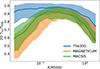 |
Fig. 6. Ratio between the SL and MW temperature profiles in different simulations. |
To further study azimuthal temperature variations in the ICM, we used 2D maps of TSL to analyse its distribution normalised by the local 1D radial profile in a given radial annulus interpolated at the position of each pixel of the 2D map (TLOC). The maps cover 4 × R500c with a grid of 400 × 400 pixels, meaning that the pixel size spans between about 9 and 18 kpc for the smallest and largest systems. This corresponds to physical scales between 1 and 4 arcsec, comparable to the size of a single pixel in the mock epic images. This approach isolates relative temperature fluctuations within clusters, allowing for a direct comparison of the spatial variability of the thermal structure, independent of the overall temperature normalisation. The use of this normalised quantity is motivated by several key trends observed in the simulations. In particular, Magneticum exhibits a more pronounced difference between TSL and TMW compared to The300 (see Fig. 6). Similarly, Magneticum shows a stronger deviation between temperature profiles reconstructed from median Voronoi temperature maps and those obtained via spectral fitting in radial bins (see Fig. F.1). These discrepancies suggest that Magneticum exhibits stronger thermal inhomogeneities and multi-phase structure in the ICM, which can enhance azimuthal variations and bias projected temperatures. This is consistent with differences in the underlying hydrodynamic schemes: SPH formulations with limited mixing are known to preserve cool substructures and generate larger temperature contrasts (e.g. Rasia et al. 2014). More recent SPH implementations, such as the improved scheme in GADGET-X used for The300, or the OWLS-based sub-grid physics adopted in MACSIS (Schaye et al. 2010) promote more efficient mixing and therefore tend to produce smoother temperature fields. By computing the probability density function (PDF) of the normalised TSL across clusters as a function of radius, we obtained a population-level diagnostic that is sensitive to such internal fluctuations. A broader distribution in this statistic reflects stronger local deviations from the median, and thus captures the degree of thermal asymmetry, clumpiness, or substructure. This method removes the need for assuming a fixed hydrostatic mass bias or one-to-one matching between clusters, it provides a flexible and robust way to compare the structural complexity of the ICM across different simulation sets and physical models. The result is shown in Fig. 7, focusing on the core and outskirts in the three simulations. We find that The300 has the tightest distribution in the core, where fluctuations are at the 40% level at most. The distribution is broader in MACSIS and especially in Magneticum, reaching also a factor of two. In the outskirts there is better agreement between the simulations, especially at the positive fluctuations end. We also notice that the PDF in Magneticum tend to peak at values slightly larger than one, possibly pointing to non-Gaussian temperature fluctuation distribution. We verified that the temperature variation expected across individual pixels from the underlying radial profile is smaller than the width of the distributions shown in Fig. 7 (see in Appendix E).
 |
Fig. 7. Comparison between the distribution of the local SL temperature fluctuations in 2D maps within different apertures for different simulations. TLOC is the 1D radial profile at the position of each pixel in the map. |
We took a further step by directly measuring the first, second, and third moments of the temperature fluctuations TSL/Tloc, namely the median μ, the standard deviation σ, and the skewness, in 30 radial bins equally distributed between 0 and 1.05 × R500c. Here, the standard deviation and skewness are computed from the distribution of pixel values of TSL/Tloc within each radial bin. In each radial bin we also measured the ratio between TSL and TMW.
We find a strong correlation between the standard deviation σ of these distributions and the ratio between the 2D TSL and TMW, as shown in Fig. 8, with a Pearson correlation coefficient of −0.76. This reflects the presence of multi-temperature gas: as the distribution broadens, gas components at different temperatures are weighted differently by the SL and MW estimators, increasing their discrepancy.
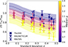 |
Fig. 8. Ratio between the SL and MW temperature profiles as a function of the standard deviation of the SL temperature fluctuations. The points are colour-coded by the median of the fluctuation distributions. |
In addition, we find a secondary trend of the temperature ratio as a function of the location parameter μ of the fitted distribution at fixed σ (Pearson coefficient of −0.49). The ratio is closer to unity for smaller μ and decreases as μ increases.
Although we do not find a clear direct correlation between the skewness and the temperature ratio (Pearson coefficient of −0.04), part of the μ dependence is reflected in the skewness. Distributions with extended tails towards lower temperatures tend to peak at higher values, corresponding to μ > 1, and describe gas distributions skewed towards colder phases, as seen for the cores of Magneticum clusters in Fig. 7. In this case, the SL weighting enhances the contribution of cold gas, reducing the ratio relative to TMW. Conversely, more symmetric or hot-skewed distributions yield ratios closer to unity.
In general, for narrow and symmetric distributions, with μ ≈ 1 and low σ, TSL is an approximately unbiased tracer of TMW. As the distribution broadens, deviations from the median become increasingly important, leading to a systematic decrease in the temperature ratio.
We modelled this behaviour with
 (3)
(3)
where 𝒩 is a Gaussian distribution and σintr represents the intrinsic scatter. The constants 1.35 and 0.22 are empirical calibration parameters determined from the global fit to the simulations; we fix them as they are only weakly constrained when left free. The functional form was chosen empirically to reproduce the flattening of the relation as a function of σ and captures the additional dependence on μ, while keeping the number of free parameters small. The numerical coefficients should therefore be interpreted as calibration parameters rather than physically meaningful quantities.
The best-fit parameters are reported in Table 2. Given measurements of μ and σ at a given radius, this model provides a mapping between the SL and MW temperatures, allowing X-ray analyses to account for unresolved multi-temperature structure in relation to the hydrostatic mass bias (Pearce et al. 2020; Ansarifard et al. 2020; Barnes et al. 2021).
In conclusion, identifying and quantifying multi-temperature structures is crucial for accurately interpreting observed temperature profiles and understanding ICM thermodynamics. One promising avenue is the use of high-resolution X-ray spectroscopy from missions like the ongoing X-Ray Imaging and Spectroscopy Mission (XRISM) or NewAthena (Cruise et al. 2025), scheduled for the next few decades. In addition to fitting a global temperature from the thermal bremsstrahlung continuum, the spectral resolution of the microcalorimeters on board these missions allows for detailed diagnostics using line ratios, particularly of the FeXXV and FeXXVI lines around 6.4–6.7 keV. These lines are sensitive to different ionisation states and thus to the plasma temperature: in a hot, single-phase plasma the FeXXVI line is prominent and comparable to FeXXV, while in cooler plasma the FeXXV line dominates (Xrism Collaboration 2025a). Importantly, the effective area of XRISM is sharply peaked at soft energies, where the folded continuum spectra of hot and cool clusters can appear deceptively similar due to instrumental response. In contrast, the iron line ratio method probes a narrow energy window where the Ancillary Response File (ARF) is approximately constant, reducing the impact of effective area variation and making it a more direct diagnostic of the thermal structure of the plasma. A discrepancy between temperatures inferred from the continuum and from line ratios would potentially indicate the presence of multi-T gas components. Such works would still need a careful treatment of systematics, as new spectral data with high signal-to-noise ratios and high resolutions may uncover limitations of the current models (see Chatzigiannakis et al. 2026).
A complementary approach will be provided by spatially resolved temperature mapping with the Wide Field Imager (WFI) on board NewAthena. While the X-ray Integral Field Unit (X-IFU) will deliver spectral diagnostics for selected regions and the brightest systems, WFI will combine a large FoV, high throughput, and improved angular resolution compared to current facilities, enabling detailed temperature maps to be constructed for large cluster samples. This will make it possible to measure the distribution of temperature fluctuations directly in observed systems, similar to the analysis presented in Fig. 7. Comparing the width, shape, and radial dependence of these distributions between observations and simulations will provide a powerful new probe of gas mixing, turbulence, accretion, and AGN feedback processes, while also offering a direct way to quantify the level of unresolved multi-temperature structure that may bias standard spectroscopic temperature measurements.
An alternative and complementary approach involves combining X-ray and SZ observations (Pointecouteau et al. 2002; Kitayama et al. 2004; Ruppin et al. 2018; Eckert et al. 2019; De Luca et al. 2021; Chappuis et al. 2025; Gavidia et al. 2026; De Luca et al. 2026). The SZ signal is proportional to the integrated electron pressure, whereas the X-ray emission is proportional to the emission measure, i.e. the gas density squared. As a result, X-ray temperatures are weighted more heavily towards denser, cooler regions, while SZ-derived temperatures reflect a more volume-averaged (or MW) thermal state. Comparing the SZ-inferred temperature, obtained by dividing the SZ pressure by the X-ray electron density or directly from the relativistic SZ signal, to the X-ray spectroscopic temperature can thus reveal discrepancies arising from multi-T structure, clumping, or non-thermal pressure support (Kay et al. 2024). In both approaches, a consistent difference between the temperature diagnostics offers a valuable observational pathway to identifying thermal complexity in the ICM.
6. Summary and conclusions
Within the context of the CHEX-MATE project (CHEX-MATE Collaboration 2021), our primary goal is to assess whether standard X-ray analysis techniques can accurately recover the true thermodynamic properties of massive galaxy clusters. To this end, we selected CHEX-MATE-like cluster samples from three state-of-the-art hydrodynamical simulations: The300 (Cui et al. 2018), Magneticum (Dolag et al. 2017), and MACSIS (Barnes et al. 2017). Using the gas particles in each simulated cluster, we generated idealised X-ray emission maps and folded them through the instrumental response of XMM-Newton using our newly developed tool, xmm_simulator, to create high-fidelity, end-to-end synthetic EPIC observations (see Sect. 3).
We then applied standard X-ray analysis tools, including routines from pyproffit (Eckert et al. 2020) and hydromass (Eckert et al. 2022), to extract surface brightness and temperature profiles, perform deprojection, and derive intrinsic 3D thermodynamic profiles (see Sect. 4). This workflow allowed for a direct, controlled comparison between the output of our X-ray analysis and the corresponding true profiles from the simulations, enabling a quantitative assessment of the accuracy of the recovery. Before summarising the implications of our findings, we emphasise that the simulated samples span a broad range of masses and redshifts and were selected to mimic the CHEX-MATE parameter space. The goal of this work is therefore not to infer properties of the cluster population as a whole, but to assess how reliably thermodynamic quantities can be recovered from realistic mock observations.
We find that the gas density profiles are robustly reconstructed across all methods and simulations, with the correct intrinsic scatter. In particular, using azimuthal median surface brightness profiles derived from Voronoi-tessellated images improves accuracy: other than some discrepancies in the core because of mis-centring effects between the peak of the X-ray emitting gas and the dark matter, the gas density profiles are reconstructed within at most 2% in all simulations. The gas masses are reconstructed to better than 1% uncertainty. The Voronoi technique suppresses the influence of localised surface brightness enhancements due to cool gas clumps, which otherwise bias the inferred density high by a few percent.
While the gas density is well-defined in simulations, defining a representative true temperature is more complex. We compared two standard weighting schemes: the SL and MW temperatures. The SL weighting provides an accurate approximation of temperatures derived from X-ray spectral fitting in annular bins. However, we observe more scatter in the temperature reconstruction compared to the density case and a systematic difference between TSL and TMW profiles, a difference that varies across simulations. This suggests that these weighting schemes carry information about the underlying physical state of the ICM. If these effects were only due to projection effects, we would expect the TMW to be higher in the core and lower in the outskirts compared to TSL. However, in our simulations, we consistently find TMW to be higher than TSL at all radii. This deviation follows expectations and points to the presence of unresolved multi-temperature gas structures, which have a significant impact on the reconstructed profiles. Even though the input and output density and temperature profiles appear consistent, the derived thermal pressure and entropy profiles differ. This discrepancy may result from an unaccounted for multi-temperature distribution in the X-ray spectral modelling combined with possible non-thermal pressure contributions.
These findings have important implications for the interpretation of hydrostatic mass estimates in galaxy clusters (see the discussions in Rasia et al. 2006, 2012; Biffi et al. 2016; Pearce et al. 2020). A long-standing issue in X-ray cluster cosmology is the hydrostatic mass bias, where masses derived under the assumption of hydrostatic equilibrium are systematically low. This discrepancy has often been attributed to non-thermal pressure support from bulk motions or turbulence in the ICM. However, recent high-resolution spectroscopic measurements from XRISM have revealed remarkably low gas velocity dispersions in relaxed systems, suggesting that non-thermal pressure is not sufficient to account for the full bias (XRISM Collaboration 2025; Xrism Collaboration 2025a,b,c; Fujita et al. 2025), though studies have only thus far examined central regions. Our results suggest an alternative and complementary explanation in line with findings from Henson et al. (2017), Pearce et al. (2020), and Barnes et al. (2021): the presence of unresolved multi-temperature structures in the ICM can bias spectroscopic temperature measurements, leading to a suppression of the inferred thermal pressure. If the temperature is underestimated due to projection effects or local cooling structures, the derived hydrostatic mass will also be biased low, even in systems that are otherwise in equilibrium. These results highlight the importance of temperature reconstruction methods that mitigate these biases, and stress the importance of multi-wavelength, spatially resolved, and dynamical analyses to disentangle the true thermodynamic state and equilibrium conditions of the ICM. Looking ahead, our findings emphasise the importance of isolating the distinct sources of bias that affect X-ray-derived cluster mass estimates. In future work, we will extend this analysis to directly compare hydrostatic mass estimates with true masses, enabling a detailed assessment of how much bias arises from assumptions of hydrostatic equilibrium, from the use of single-temperature models in a multi-phase medium, and from projection effects such as triaxiality and line-of-sight substructure (Kim et al. 2024; Saxena et al. 2025; Chappuis et al. 2025). This will be key to understanding whether the observed hydrostatic mass bias truly reflects a breakdown of equilibrium in the ICM, or whether it stems, at least in part, from systematic limitations in our current X-ray analysis methodologies.
Acknowledgments
RS and DE are supported by Swiss National Science Foundation project grant #200021_212576. ER is partially supported by the NASA -EGIP Grant 80NSSC25K8009. EP acknowledges support of CNES, the French space agency and from the French Agence Nationale de la Recherche (ANR), under grant ANR-22-CE31-0010. VB acknowledges partial support from the INAF Grant 2023 “Origins of the ICM metallicity in galaxy clusters”. This research was supported by the International Space Science Institute (ISSI) in Bern, through ISSI International Team project #565 (Multi-Wavelength Studies of the Culmination of Structure Formation in the Universe). We acknowledge the financial contribution from the contracts Prin-MUR 2022 supported by Next Generation EU (M4.C2.1.1, n.20227RNLY3 The concordance cosmological model: stress-tests with galaxy clusters), and from the European Union’s Horizon 2020 Programme under the AHEAD2020 project (grant agreement n. 871158). MDP acknowledges financial support from PRIN-MUR grant 20228B938N Mass and selection biases of galaxy clusters: a multi-probe approach funded by the European Union Next generation EU, Mission 4 Component 2 CUP B53D23004790006. MS acknowledges financial contributions from contract ASI-INAF n.2017-14-H.0, contract INAF mainstream project 1.05.01.86.10, INAF Theory Grant 2023: Gravitational lensing detection of matter distribution at galaxy cluster boundaries and beyond (1.05.23.06.17). MR acknowledges the financial contribution from INAF grant 1.05.24.02.10 LL acknowledges the financial contribution from the INAF grant 1.05.12.04.01. MG acknowledges support from the ERC Consolidator Grant BlackHoleWeather (101086804). JS was supported by NASA Astrophysics Data Analysis Program (ADAP) Grant 80NSSC21K1571. HB, FDL, PM acknowledge the support by INFN through the InDark initiative. The authors thank the anonymous referee for their helpful comments that improved the quality of the article.
References
- Abbott, T. M. C., Aguena, M., Alarcon, A., et al. 2020, Phys. Rev. D, 102, 023509 [Google Scholar]
- Allen, S. W., Schmidt, R. W., Ebeling, H., Fabian, A. C., & van Speybroeck, L. 2004, MNRAS, 353, 457 [NASA ADS] [CrossRef] [Google Scholar]
- Ansarifard, S., Rasia, E., Biffi, V., et al. 2020, A&A, 634, A113 [NASA ADS] [CrossRef] [EDP Sciences] [Google Scholar]
- Arnaud, K. A. 1996, ASP Conf. Ser., 101, 17 [Google Scholar]
- Asplund, M., Grevesse, N., Sauval, A. J., & Scott, P. 2009, ARA&A, 47, 481 [NASA ADS] [CrossRef] [Google Scholar]
- Bahar, Y. E., Bulbul, E., Ghirardini, V., et al. 2024, A&A, 691, A188 [NASA ADS] [CrossRef] [EDP Sciences] [Google Scholar]
- Barnes, D. J., Kay, S. T., Henson, M. A., et al. 2017, MNRAS, 465, 213 [Google Scholar]
- Barnes, D. J., Vogelsberger, M., Pearce, F. A., et al. 2021, MNRAS, 506, 2533 [NASA ADS] [CrossRef] [Google Scholar]
- Bartalucci, I., Molendi, S., Rasia, E., et al. 2023, A&A, 674, A179 [NASA ADS] [CrossRef] [EDP Sciences] [Google Scholar]
- Battaglia, N., Bond, J. R., Pfrommer, C., & Sievers, J. L. 2013, ApJ, 777, 123 [NASA ADS] [CrossRef] [Google Scholar]
- Beauchesne, B., Clément, B., Hibon, P., et al. 2024, MNRAS, 527, 3246 [Google Scholar]
- Beck, A. M., Murante, G., Arth, A., et al. 2016, MNRAS, 455, 2110 [Google Scholar]
- Behroozi, P., Wechsler, R., & Wu, H.-Y. 2013, ApJ, 762, 109 [NASA ADS] [CrossRef] [Google Scholar]
- Biffi, V., Dolag, K., Böhringer, H., & Lemson, G. 2012, MNRAS, 420, 3545 [NASA ADS] [Google Scholar]
- Biffi, V., Dolag, K., & Böhringer, H. 2013, MNRAS, 428, 1395 [Google Scholar]
- Biffi, V., Borgani, S., Murante, G., et al. 2016, ApJ, 827, 112 [NASA ADS] [CrossRef] [Google Scholar]
- Bleem, L. E., Bocquet, S., Stalder, B., et al. 2020, ApJS, 247, 25 [Google Scholar]
- Böhringer, H., Schuecker, P., Guzzo, L., et al. 2004, A&A, 425, 367 [NASA ADS] [CrossRef] [EDP Sciences] [Google Scholar]
- Booth, C. M., & Schaye, J. 2009, MNRAS, 398, 53 [Google Scholar]
- Braspenning, J., Schaye, J., Schaller, M., Kugel, R., & Kay, S. T. 2025, MNRAS, 536, 3784 [Google Scholar]
- Bryan, G. L., & Norman, M. L. 1998, ApJ, 495, 80 [NASA ADS] [CrossRef] [Google Scholar]
- Bulbul, E., Liu, A., Kluge, M., et al. 2024, A&A, 685, A106 [NASA ADS] [CrossRef] [EDP Sciences] [Google Scholar]
- Campitiello, M. G., Ettori, S., Lovisari, L., et al. 2022, A&A, 665, A117 [NASA ADS] [CrossRef] [EDP Sciences] [Google Scholar]
- Cash, W. 1979, ApJ, 228, 939 [Google Scholar]
- Chappuis, L., Eckert, D., Sereno, M., et al. 2025, A&A, 699, A141 [NASA ADS] [CrossRef] [EDP Sciences] [Google Scholar]
- Chatzigiannakis, D., Pillepich, A., Simionescu, A., Truong, N., & Nelson, D. 2026, MNRAS, 547, stag061 [Google Scholar]
- CHEX-MATE Collaboration (Arnaud, M., et al.) 2021, A&A, 650, A104 [NASA ADS] [CrossRef] [EDP Sciences] [Google Scholar]
- Clerc, N., & Finoguenov, A. 2022, ArXiv e-prints [arXiv:2203.11906] [Google Scholar]
- Croston, J. H., Pratt, G. W., Böhringer, H., et al. 2008, A&A, 487, 431 [NASA ADS] [CrossRef] [EDP Sciences] [Google Scholar]
- Cruise, M., Guainazzi, M., Aird, J., et al. 2025, Nat. Astron., 9, 36 [Google Scholar]
- Cui, W., Knebe, A., Yepes, G., et al. 2018, MNRAS, 480, 2898 [Google Scholar]
- De Luca, F., De Petris, M., Yepes, G., et al. 2021, MNRAS, 504, 5383 [NASA ADS] [CrossRef] [Google Scholar]
- De Luca, F., Bourdin, H., Mazzotta, P., et al. 2026, A&A, 707, A32 [NASA ADS] [CrossRef] [EDP Sciences] [Google Scholar]
- Diehl, S., & Statler, T. S. 2006, MNRAS, 368, 497 [NASA ADS] [CrossRef] [Google Scholar]
- Dolag, K. 2015, IAU General Assembly, 29, 2250156 [Google Scholar]
- Dolag, K., Borgani, S., Murante, G., & Springel, V. 2009, MNRAS, 399, 497 [Google Scholar]
- Dolag, K., Mevius, E., & Remus, R.-S. 2017, Galaxies, 5, 35 [NASA ADS] [CrossRef] [Google Scholar]
- Dolag, K., Remus, R.-S., Valenzuela, L. M., et al. 2025, A&A, accepted [arXiv:2504.01061] [Google Scholar]
- Eckert, D., Ghirardini, V., Ettori, S., et al. 2019, A&A, 621, A40 [NASA ADS] [CrossRef] [EDP Sciences] [Google Scholar]
- Eckert, D., Finoguenov, A., Ghirardini, V., et al. 2020, Open J. Astrophys., 3, 12 [NASA ADS] [CrossRef] [Google Scholar]
- Eckert, D., Ettori, S., Pointecouteau, E., van der Burg, R. F. J., & Loubser, S. I. 2022, A&A, 662, A123 [NASA ADS] [CrossRef] [EDP Sciences] [Google Scholar]
- Euclid Collaboration (Giocoli, C., et al.) 2024, A&A, 681, A67 [NASA ADS] [CrossRef] [EDP Sciences] [Google Scholar]
- Evrard, A. E., Metzler, C. A., & Navarro, J. F. 1996, ApJ, 469, 494 [Google Scholar]
- Fabjan, D., Borgani, S., Tornatore, L., et al. 2010, MNRAS, 401, 1670 [Google Scholar]
- Fujita, Y., Fukushima, K., Sato, K., Fukazawa, Y., & Kondo, M. 2025, PASJ, 77, S270 [Google Scholar]
- Gardini, A., Rasia, E., Mazzotta, P., et al. 2004, MNRAS, 351, 505 [Google Scholar]
- Gaspari, M., Tombesi, F., & Cappi, M. 2020, Nat. Astron., 4, 10 [Google Scholar]
- Gavidia, A., Kim, J., Sayers, J., et al. 2026, A&A, 710, A40 [NASA ADS] [CrossRef] [EDP Sciences] [Google Scholar]
- Ghirardini, V., Eckert, D., Ettori, S., et al. 2019, A&A, 621, A41 [NASA ADS] [CrossRef] [EDP Sciences] [Google Scholar]
- Ghirardini, V., Bulbul, E., Artis, E., et al. 2024, A&A, 689, A298 [NASA ADS] [CrossRef] [EDP Sciences] [Google Scholar]
- Gianfagna, G., De Petris, M., Yepes, G., et al. 2021, MNRAS, 502, 5115 [NASA ADS] [CrossRef] [Google Scholar]
- Gianfagna, G., Rasia, E., Cui, W., et al. 2023, MNRAS, 518, 4238 [Google Scholar]
- Giocoli, C., Despali, G., Meneghetti, M., et al. 2025, A&A, 697, A184 [NASA ADS] [CrossRef] [EDP Sciences] [Google Scholar]
- Gupta, N., Saro, A., Mohr, J. J., Dolag, K., & Liu, J. 2017, MNRAS, 469, 3069 [Google Scholar]
- Henson, M. A., Barnes, D. J., Kay, S. T., McCarthy, I. G., & Schaye, J. 2017, MNRAS, 465, 3361 [NASA ADS] [CrossRef] [Google Scholar]
- Hilton, M., Sifón, C., Naess, S., et al. 2021, ApJS, 253, 3 [Google Scholar]
- Hirschmann, M., Dolag, K., Saro, A., et al. 2014, MNRAS, 442, 2304 [Google Scholar]
- Jennings, F., & Davé, R. 2023, MNRAS, 526, 1367 [NASA ADS] [CrossRef] [Google Scholar]
- Kawahara, H., Suto, Y., Kitayama, T., et al. 2007, ApJ, 659, 257 [NASA ADS] [CrossRef] [Google Scholar]
- Kay, S. T., Braspenning, J., Chluba, J., et al. 2024, MNRAS, 534, 251 [Google Scholar]
- Kim, J., Sayers, J., Sereno, M., et al. 2024, A&A, 686, A97 [NASA ADS] [CrossRef] [EDP Sciences] [Google Scholar]
- Kitayama, T., Komatsu, E., Ota, N., et al. 2004, PASJ, 56, 17 [NASA ADS] [Google Scholar]
- Klypin, A., Yepes, G., Gottlöber, S., Prada, F., & Heß, S. 2016, MNRAS, 457, 4340 [Google Scholar]
- Knollmann, S. R., & Knebe, A. 2009, ApJS, 182, 608 [Google Scholar]
- Komatsu, E., Smith, K. M., Dunkley, J., et al. 2011, ApJS, 192, 18 [Google Scholar]
- Kravtsov, A. V., & Borgani, S. 2012, ARA&A, 50, 353 [Google Scholar]
- Lau, E. T., Kravtsov, A. V., & Nagai, D. 2009, ApJ, 705, 1129 [NASA ADS] [CrossRef] [Google Scholar]
- Lehmer, B. D., Xue, Y. Q., Brandt, W. N., et al. 2012, ApJ, 752, 46 [NASA ADS] [CrossRef] [Google Scholar]
- Lesci, G. F., Marulli, F., Moscardini, L., et al. 2025, A&A, 703, A25 [NASA ADS] [CrossRef] [EDP Sciences] [Google Scholar]
- Lovisari, L., Ettori, S., Rasia, E., et al. 2024, A&A, 682, A45 [NASA ADS] [CrossRef] [EDP Sciences] [Google Scholar]
- Mathiesen, B. F., & Evrard, A. E. 2001, ApJ, 546, 100 [CrossRef] [Google Scholar]
- Mazzotta, P., Rasia, E., Moscardini, L., & Tormen, G. 2004, MNRAS, 354, 10 [NASA ADS] [CrossRef] [Google Scholar]
- McCarthy, I. G., Schaye, J., Bird, S., & Le Brun, A. M. C. 2017, MNRAS, 465, 2936 [Google Scholar]
- Meneghetti, M., Rasia, E., Merten, J., et al. 2010, A&A, 514, A93 [NASA ADS] [CrossRef] [EDP Sciences] [Google Scholar]
- Meneghetti, M., Fedeli, C., Zitrin, A., et al. 2011, A&A, 530, A17 [NASA ADS] [CrossRef] [EDP Sciences] [Google Scholar]
- Miyazaki, S., Oguri, M., Hamana, T., et al. 2018, PASJ, 70, S27 [NASA ADS] [Google Scholar]
- Mo, H. J., & White, S. D. M. 2002, MNRAS, 336, 112 [Google Scholar]
- Muñoz-Echeverría, M., Macías-Pérez, J. F., Pratt, G. W., et al. 2024, A&A, 682, A147 [NASA ADS] [CrossRef] [EDP Sciences] [Google Scholar]
- Muñoz-Echeverría, M., Pointecouteau, E., Pratt, G. W., et al. 2025, A&A, 704, A302 [Google Scholar]
- Nagai, D., Vikhlinin, A., & Kravtsov, A. V. 2007, ApJ, 655, 98 [Google Scholar]
- Navarro, J. F., Frenk, C. S., & White, S. D. M. 1996, ApJ, 462, 563 [Google Scholar]
- Nelson, K., Lau, E. T., Nagai, D., Rudd, D. H., & Yu, L. 2014, ApJ, 782, 107 [NASA ADS] [CrossRef] [Google Scholar]
- Pearce, F. A., Kay, S. T., Barnes, D. J., Bower, R. G., & Schaller, M. 2020, MNRAS, 491, 1622 [NASA ADS] [CrossRef] [Google Scholar]
- Pierre, M., Pacaud, F., Adami, C., et al. 2016, A&A, 592, A1 [NASA ADS] [CrossRef] [EDP Sciences] [Google Scholar]
- Planck Collaboration XIII. 2016, A&A, 594, A13 [NASA ADS] [CrossRef] [EDP Sciences] [Google Scholar]
- Planck Collaboration XVI. 2014, A&A, 571, A16 [NASA ADS] [CrossRef] [EDP Sciences] [Google Scholar]
- Planck Collaboration XXVII. 2016, A&A, 594, A27 [NASA ADS] [CrossRef] [EDP Sciences] [Google Scholar]
- Pointecouteau, E., Hattori, M., Neumann, D., et al. 2002, A&A, 387, 56 [NASA ADS] [CrossRef] [EDP Sciences] [Google Scholar]
- Popesso, P., Marini, I., Dolag, K., et al. 2025, A&A, 704, A278 [NASA ADS] [CrossRef] [EDP Sciences] [Google Scholar]
- Pratt, G. W., Arnaud, M., Biviano, A., et al. 2019, Space Sci. Rev., 215, 25 [Google Scholar]
- Pratt, G. W., Arnaud, M., Maughan, B. J., & Melin, J.-B. 2022, A&A, 665, A24 [NASA ADS] [CrossRef] [EDP Sciences] [Google Scholar]
- Predehl, P., Andritschke, R., Arefiev, V., et al. 2021, A&A, 647, A1 [EDP Sciences] [Google Scholar]
- Rasia, E., Ettori, S., Moscardini, L., et al. 2006, MNRAS, 369, 2013 [CrossRef] [Google Scholar]
- Rasia, E., Mazzotta, P., Bourdin, H., et al. 2008, ApJ, 674, 728 [Google Scholar]
- Rasia, E., Meneghetti, M., Martino, R., et al. 2012, New J. Phys., 14, 055018 [Google Scholar]
- Rasia, E., Lau, E. T., Borgani, S., et al. 2014, ApJ, 791, 96 [NASA ADS] [CrossRef] [Google Scholar]
- Rasia, E., Borgani, S., Murante, G., et al. 2015, ApJ, 813, L17 [Google Scholar]
- Rasia, E., Tripodi, R., Borgani, S., et al. 2025, A&A, 702, A182 [NASA ADS] [CrossRef] [EDP Sciences] [Google Scholar]
- Remus, R.-S., Dolag, K., Naab, T., et al. 2017, MNRAS, 464, 3742 [Google Scholar]
- Riva, G., Pratt, G. W., Rossetti, M., et al. 2024, A&A, 691, A340 [NASA ADS] [CrossRef] [EDP Sciences] [Google Scholar]
- Rossetti, M., Eckert, D., Gastaldello, F., et al. 2024, A&A, 686, A68 [NASA ADS] [CrossRef] [EDP Sciences] [Google Scholar]
- Ruppin, F., Mayet, F., Pratt, G. W., et al. 2018, A&A, 615, A112 [NASA ADS] [CrossRef] [EDP Sciences] [Google Scholar]
- Rykoff, E. S., Rozo, E., Busha, M. T., et al. 2014, ApJ, 785, 104 [Google Scholar]
- Saxena, H., Sayers, J., Gavidia, A., et al. 2025, A&A, 700, A128 [NASA ADS] [CrossRef] [EDP Sciences] [Google Scholar]
- Schaye, J., & Dalla Vecchia, C. 2008, MNRAS, 383, 1210 [Google Scholar]
- Schaye, J., Dalla Vecchia, C., Booth, C. M., et al. 2010, MNRAS, 402, 1536 [Google Scholar]
- Scheck, D., Sanders, J. S., Biffi, V., et al. 2023, A&A, 670, A33 [NASA ADS] [CrossRef] [EDP Sciences] [Google Scholar]
- Sereno, M., Maurogordato, S., Cappi, A., et al. 2025, A&A, 693, A2 [NASA ADS] [CrossRef] [EDP Sciences] [Google Scholar]
- Springel, V. 2005, MNRAS, 364, 1105 [Google Scholar]
- Springel, V., & Hernquist, L. 2003, MNRAS, 339, 289 [Google Scholar]
- Staniszewski, Z., Ade, P. A. R., Aird, K. A., et al. 2009, ApJ, 701, 32 [CrossRef] [Google Scholar]
- Steinborn, L. K., Dolag, K., Hirschmann, M., Prieto, M. A., & Remus, R.-S. 2015, MNRAS, 448, 1504 [Google Scholar]
- Sutherland, R. S., & Dopita, M. A. 1993, ApJS, 88, 253 [Google Scholar]
- Teklu, A. F., Remus, R.-S., Dolag, K., et al. 2015, ApJ, 812, 29 [Google Scholar]
- Tornatore, L., Borgani, S., Dolag, K., & Matteucci, F. 2007, MNRAS, 382, 1050 [Google Scholar]
- Ueda, Y., Akiyama, M., Hasinger, G., Miyaji, T., & Watson, M. G. 2014, ApJ, 786, 104 [Google Scholar]
- Virtanen, P., Gommers, R., Oliphant, T. E., et al. 2020, Nat. Methods, 17, 261 [Google Scholar]
- Wicker, R., Douspis, M., Salvati, L., & Aghanim, N. 2023, A&A, 674, A48 [NASA ADS] [CrossRef] [EDP Sciences] [Google Scholar]
- Wiersma, R. P. C., Schaye, J., Theuns, T., Dalla Vecchia, C., & Tornatore, L. 2009, MNRAS, 399, 574 [NASA ADS] [CrossRef] [Google Scholar]
- XRISM Collaboration (Audard, M., et al.) 2025, Nature, 638, 365 [Google Scholar]
- Xrism Collaboration (Audard, M., et al.) 2025a, ApJ, 985, L20 [Google Scholar]
- Xrism Collaboration (Audard, M., et al.) 2025b, ApJ, 982, L5 [Google Scholar]
- Xrism Collaboration (Audard, M., et al.) 2025c, PASJ, 77, S242 [Google Scholar]
- ZuHone, J., Bahar, Y. E., Biffi, V., et al. 2023, A&A, 675, A150 [NASA ADS] [CrossRef] [EDP Sciences] [Google Scholar]
The virial mass is the total mass enclosed within the virial radius, i.e. a region encompassing an average overdensity that is equal to the critical density of the Universe at the cluster redshift multiplied by the virial overdensity (see Bryan & Norman 1998). At z = 0 Δvir is about 99 times larger than the critical density and 330 times larger than the background matter density in vanilla Λ cold dark matter.
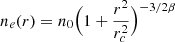 .
.
Appendix A: Gas density and gas mass
We further investigate the reconstruction of gas density profiles and gas mass in this appendix. Figure A.1 shows the gas density reconstruction for one of The300 clusters. The true profile is shown in black, the reconstructed ones, including the Voronoi binning technique, are shown in light blue and red. The bottom panel shows the ratio to the true profile, highlighting the better precision of the profile reconstructed from the Voronoi binned image, with local deviations of at most 5%.
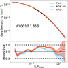 |
Fig. A.1. Density profile reconstruction of CL0017.1.119 from The300 simulation. |
A detailed comparison is presented in Fig. A.2, where each of the three main panels corresponds to one simulation set. In each case, the top panel displays the gas density profiles reconstructed using the NFW, NP, and FM methods. The middle panel shows the ratio between the azimuthal median reconstructed and true profiles for each method, as derived from the Voronoi-binned images. The bottom panel presents the ratio between the profiles measured directly from the mock EPIC images and the true profiles. Overall, we find excellent agreement among the density profiles recovered with the three methods. The median surface brightness profiles extracted from the Voronoi images closely follow the one-to-one relation with the true profiles. In contrast, the direct analysis of the mock EPIC images tends to overestimate the gas density by approximately 5%. This result confirms that the Voronoi-based approach enables an unbiased recovery of the gas density profile, owing to its reduced sensitivity to surface brightness fluctuations caused by substructures or colder gas clumps whose emission is not prominent enough to be masked during preprocessing. The profiles in Magneticum tend to have lower normalisation and a flatter slope. This is expected given the slightly different mass selection (see Sect. 2.4), because more massive clusters typically show steeper profiles (see e.g. Croston et al. 2008; Pratt et al. 2022). We conclude that despite the intrinsic differences between individual simulations, our methods are able to properly reconstruct the gas density profiles independently of their specific shape.
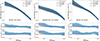 |
Fig. A.2. Deprojected 3D gas density profiles. Each column corresponds to one simulation: The300 (left), Magneticum (centre), and MACSIS (right). The colours denote the three reconstruction methods. The smaller central (bottom) panels show the ratio between the median Voronoi (the standard mean) profile and the true input one. |
We estimated the total gas mass content in our mock clusters and compared it to the true value in the hydrodynamical simulations. The gas mass was computed by integrating the electron number density, following
 (A.1)
(A.1)
where μe is the mean electron molecular weight and mp is the proton mass. In particular, we converted the gas particle number density to total gas mass in units of solar masses by computing the mean molecular weight per electron in a flexible way based on the chosen abundance table with the latest version of hydromass. For consistency with the generated boxes (see Sect. 3) we used the abundances from Asplund et al. (2009), which gives μe = 1.146. Figure A.3 shows the comparison between the measured and true total gas mass within the true R500c in all three simulations. The panel refers to the gas mass estimated from the integral of the Voronoi azimuthal median (mean surface brightness) density profile. When combining the three simulation, the median ratio between measured and true gas mass is 0.993, with 16th and 84th percentile points at 0.916, and 1.067, meaning that the gas mass reconstruction is precise within 1% and a cluster to cluster scatter variation of about 7.5%. We ran a linear regression algorithm using scipy on the logarithm of the gas masses, accounting for a zero point of 14.0 on both axis. Overall, we find excellent agreement with the one to one relation. The best-fit slope is closer to one especially for The300 and Magneticum using the median Voronoi profiles. The fit is less accurate for MACSIS, which lacking the Tier1 mass objects has a limited mass range. We find the residuals to scatter around the mean relation by 0.027 (0.021, 0.022) dex in The300 (Magneticum, MACSIS). The gas mass is overestimated by about 5% using the standard count rate images, this is expected as we also show that the gas density is overestimated at similar levels in the previous section. We report all parameters in Table A.2. We conclude that our methods are able to properly reconstruct the total gas mass in CHEX-MATE-like cluster samples.
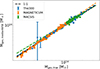 |
Fig. A.3. Comparison between the measured and true gas mass within R500c. The masses were inferred from the Voronoi-tessellated images. The dashed coloured lines denote the best linear fit to each simulation. |
Best-fit beta model parameters of the gas density profiles in our simulations.
Best linear fit parameters of the gas mass recovery in our simulations.
Appendix B: Thermodynamical profiles
In this appendix we collect additional results about X-ray observables, starting with temperature. Figure B.1 is about the temperature profile reconstruction in MACSIS (Sect. 5.2): it is the ratio between the model of the temperature profile and the measured one, for different reconstruction methods. It shows how the modelling is able to reproduce the measurement, and confirms that the temperature bias in the core of MACSIS (Fig. 5) is due to the measurement (see also Fig. 4) and not due to the modelling itself. In any case, despite some discrepancies along the profile, the global recovery of the temperature within R500c is robust, and in excellent agreement with the one-to-one expectation, as shown in Fig. B.2. We quantified the temperature recovery by fitting a linear relation between output and input temperatures. We find slopes close to unity, with values of 0.99±0.01, 1.02±0.01, and 1.01±0.01, respectively, for The300, MAGNETICUM, and MACSIS. Figure B.3 is about corner plot showing the best-fit parameters of the model describing the ratio between MW and SL temperatures in Sect. 5.2.2 (see Eq. 3).
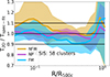 |
Fig. B.1. Ratio between the reconstructed 2D temperature profile with NFW, NP, and FM models to the result of the X-ray spectral fitting in MACSIS. |
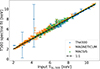 |
Fig. B.2. Comparison between the SL temperature estimated within R500c and that estimated from the modelled temperature profile within the true R500c. |
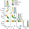 |
Fig. B.3. Corner plot with the marginalised 1D posterior distribution of the parameters describing the ratio between the SL and MW temperature as a function of median and width of the temperature fluctuation distribution. |
We then focused on derived observables, i.e. the ones that are not directly measured on the X-ray data, such as surface brightness and temperature, as well as the gas pressure and entropy. The true pressure and entropy profiles are computed using MW quantities, obtained by averaging gas properties within each radial bin with weights proportional to the gas particle masses. They are respectively reported in Figs. B.4 and B.5.
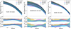 |
Fig. B.4. Deprojected 3D electron pressure profiles. Each column corresponds to one simulation: The300 (left), Magneticum (centre), and MACSIS (right). The colours denote the three reconstruction methods. The smaller central (bottom) panels show the ratio between the median Voronoi (the standard mean) profile and the true input one. |
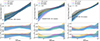 |
Fig. B.5. Deprojected 3D gas entropy profiles. Each column corresponds to one simulation: The300 (left), Magneticum (centre), and MACSIS (right). The colours denote the three reconstruction methods. The smaller central (bottom) panels show the ratio between the median Voronoi (the standard mean) profile and the true input one. |
We find that both the thermal pressure and entropy profiles recovered from the X-ray analysis are systematically underestimated relative to the true values from the simulations. Among the three simulation suites, The300 exhibits the smallest discrepancies: the thermal pressure is underestimated by approximately 10% across the entire radial range, while the entropy profile closely matches the true values beyond 0.2×R_500c and is underestimated by about 10% in the core. Both quantities remain consistent with the one-to-one relation within 1σ uncertainties. In Magneticum, the discrepancies are more pronounced. Thermal pressure is systematically underestimated by about 20% across the full profile when using the NFW and FM reconstruction methods, while the NP approach shows a smaller discrepancy (about 10%) around 0.4R500c but exhibits even larger deviations in both the core and outskirts. A similar pattern is observed for entropy, although the reconstructed values converge more closely to the true values near R500c. In MACSIS, the thermal pressure profile is moderately biased low by about 15%, while the entropy profile shows a level of disagreement similar to that seen in Magneticum. However, the three reconstruction methods yield more consistent results. In summary, the degree of agreement between the inferred and true thermodynamic profiles varies across simulations and partially depends on the reconstruction method employed. These results highlight the sensitivity of X-ray-derived pressure and entropy profiles to both physical modelling in simulations and methodological assumptions in the analysis pipeline. Understanding the origin of these discrepancies is essential, as both quantities play a central role in characterising the thermodynamic state of the ICM and in deriving cluster masses under the assumption of hydrostatic equilibrium.
The thermal pressure profile is proportional to the electron number density and the gas temperature, through the Boltzmann constant under the assumption of the ideal gas law. Since our density profiles are accurately recovered, as shown in Sect. 5, the bias in pressure is primarily driven by the thermodynamic structure of the gas. In the presence of multi-phase gas, thermodynamic quantities derived from X-ray observations are affected by non-trivial weighting and correlations between density and temperature fluctuations (e.g. Rasia et al. 2006; Nagai et al. 2007). Therefore, the discrepancy between reconstructed and true pressure profiles reflects both the bias in the reconstructed temperature encoded in unresolved multi-phase structure, which introduces correlated fluctuations that are not captured by the reconstruction. In addition, the hydrostatic mass modelling used in the temperature reconstruction assumes that the ICM is in equilibrium with the gravitational potential, neglecting any non-thermal pressure support from turbulence, bulk motions, or cosmic rays. If non-thermal pressure contributes significantly to the total pressure budget, the inferred temperature profile from a purely hydrostatic model will be suppressed to compensate, leading to an underestimation of thermal pressure. However, in this case the input pressure is only thermal, i.e. the one computed from the ideal gas law starting from density and temperature. Therefore, any inconsistency in the recovery of thermal pressure is not due to the non-thermal component in this work. In addition, the assumption of spherical symmetry in the hydrostatic analysis may not hold in detail: triaxiality of the halo and projection along preferential axes can distort both the density and temperature gradient estimates and thus affect the pressure reconstruction.
Entropy is directly (inversely) proportional to temperature (density to the two-thirds power). It is a derived quantity that inherits biases from both temperature and density. Entropy is particularly sensitive to the thermal history of the ICM and is therefore more susceptible to localised structures, cooling clumps, or feedback-induced perturbations that may not be properly accounted for in the deprojection process under the assumption of single-temperature ICM within the framework of hydrostatic mass modelling. As a result, entropy profiles are especially affected by unresolved structure and deviations from the single-temperature assumption in the deprojection.
Future work will focus on dissecting these contributions in more detail by comparing hydrostatic mass reconstructions to the true simulation masses, investigating the impact of different temperature reconstruction schemes, and exploring projection effects due to triaxiality and substructure. Such an analysis is essential to calibrate cluster thermodynamics for cosmological applications and to refine our interpretation of the hydrostatic mass bias.
Appendix C: Impact of mass and redshift selection
One of the potential limitations of our analysis is that the simulated cluster samples span different ranges in mass and redshift. This can introduce apparent differences between simulations that are not intrinsic to the modelling, but instead driven by selection effects. To assess the robustness of our results, we repeated part of the analysis using subsamples matched in mass and redshift across the different simulation suites. This allowed us to isolate the impact of observational recovery from variations induced by the underlying cluster population. We defined two representative regions in the M500c − −z plane: 14.5 ≤ log10(M500c/M⊙)≤14.9 and 0.05 ≤ z ≤ 0.22 (Sel1); and 14.9 ≤ log10(M500c/M⊙)≤15.05 and 0.2 ≤ z ≤ 0.36 (Sel2.) Sel1 yields 47 (45, 38) clusters for CHEX-MATE (The300, MAGNETICUM). Sel2 yields 20 (22, 10, 25) clusters for CHEX-MATE (The300, MAGNETICUM, MACSIS). Figure C.1 shows the distribution of clusters in the mass–redshift plane, together with the regions used for the matched selections.
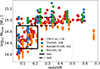 |
Fig. C.1. Equivalent to Fig. 1, with the addition of two sub-selections designed to test selection effects related to mass and redshift. |
We report the reconstruction of density profiles for the matched samples in Fig. C.2. We find similar trends as in Fig. A.2, with MAGNETICUM having a lower normalisation, even though the samples are now in the same true mass range. The results confirm the accuracy of the density reconstruction, consistent with the full-sample analysis. Similarly, the behaviour of the temperature profiles and the offset between different weighting schemes are preserved. By restricting the analysis to narrower bins in mass and redshift, we reduced the contribution of population variance to the measured scatter. We find that the reconstruction of the scatter remains accurate, consistently with that from the full sample, indicating that our reconstruction is not artificially driven by the broad range of cluster properties.
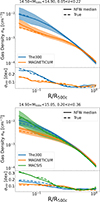 |
Fig. C.2. Equivalent to Fig. A.2, relative to two subsamples selected to test the impact of mass and redshift on density profiles. |
We find similar results for the temperature profiles. We conclude that we do not find evidence that the differences observed between simulations in Figs. A.2 and 5 are driven by selection effects. Finally, we did not find clear deviations in the temperature fluctuation distribution in Fig. 7 and the matched subsamples. Although the amplitude of the fluctuations can vary with mass and redshift, the relative behaviour of the different simulation suites is preserved after matching the samples. This indicates that the simulation-to-simulation differences discussed in Sect. 5.2.2 cannot be explained solely by the different mass and redshift distributions of the underlying samples, but instead reflect intrinsic properties of the ICM and their impact on the X-ray measurement.
Overall, these tests demonstrate that the main conclusions of this work are not driven by differences in the mass and redshift distributions of the simulated samples. Instead, they reflect the intrinsic performance of X-ray analysis techniques in recovering the underlying thermodynamic properties of galaxy clusters. This appendix further supports our interpretation of the simulations as controlled experiments to validate the recovery of physical quantities, rather than as objects of direct comparison.
Appendix D: Multi-T gas: A toy model
To explore projection effects on the cluster temperature profile in a controlled setting, we constructed a toy model under the assumption of a spherically symmetric, single-temperature structure. This does not imply that the temperature profile is flat, but rather that the gas follows a single, smooth, and radially dependent profile without azimuthal or multi-phase complexity. We then projected this 3D temperature distribution along the line of sight using both the SL and MW weighting schemes (see Eq. 2). The gas density profile was modelled with a standard β-model assuming β = 2/3 and a core radius of rc = 0.1 × R500c. Our toy model includes a CC and an outer decline and is parametrised by
![Mathematical equation: $$ \begin{aligned} T(r) = T_0 \times (1-A\exp [-(r/r_{c1})^{1.5}]) \times (1+(r/r_{c2})^2)^{-0.3}, \end{aligned} $$](/articles/aa/full_html/2026/07/aa58537-25/aa58537-25-eq11.gif) (D.1)
(D.1)
with T0 = 7 keV, A = 0.5, rc1 = 0.1, and rc2 = 0.5. The projection is performed by looping over the radial grid, computing the line-of-sight depth corresponding to each projected radius, and integrating the temperature profile in Eq. D.1 with the appropriate SL or MW weights within each shell, so that the difference between the weighting schemes only applies to the projection.
The result is shown in Fig. D.1. We find that in the central region within 0.1×R500c, the MW projection yields higher temperatures than the SL projection. This behaviour arises because the SL weighting scheme gives more emphasis to lower-temperature gas, which is prevalent in the core, thereby biasing the projected temperature downwards. Moving towards the outskirts, the density profile steepens and the line-of-sight integration length shortens, reducing the total amount of gas contributing to the projection. In this regime, the SL weighting becomes increasingly sensitive to the denser, hotter gas located in the inner portion of the shell due to its scaling with gas density squared. In contrast, the MW scheme continues to weight gas linearly by mass, giving more equal importance across the shell. As a result, the SL temperature can exceed the MW value beyond the core. At large radii beyond 3×R500c, the line-of-sight depth becomes small and the integrated signal is dominated by local gas, making the two weighting schemes converge and the MW/SL ratio approach unity. These trends arise purely from projection effects applied to a spherically symmetric, single-temperature model.
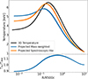 |
Fig. D.1. Spherical isothermal toy model of the gas temperature profile, including its projections along the line of sight assuming the SL and MW temperature schemes. |
Appendix E: Pixel size and radial gradients
The temperature fluctuations shown in Fig. 7 are measured on pixelised maps and can in principle be affected by the underlying radial temperature gradient across a pixel. To quantify this effect, we estimated the minimum fractional temperature variation expected from the smooth radial profile alone across the pixel as
 (E.1)
(E.1)
where Δrpix is the pixel size in units of R500c. This quantity represents the fractional temperature change across a pixel due solely to the radial gradient.
The radial dependence of δgrad is shown in Fig. E.1. We find that δgrad is largest in the innermost regions, reaching values of ∼0.1 in Magneticum and MACSIS and a few percent in The300, reflecting the steeper core temperature profiles of the first two simulations. However, δgrad rapidly decreases with radius and is < 0.01 beyond 0.2 R500c for all models. This demonstrates that while finite pixel size and the radial temperature gradient can contribute to the width of the fluctuation distributions in the very central regions, they are negligible at larger radii. In addition, we note that this estimate represents a conservative upper limit to the impact of the radial gradient. In practice, each pixel contains emission integrated along the line of sight and over a finite volume, which partially averages out the radial variation. Therefore, the effective contribution of the radial gradient to the observed fluctuations is expected to be smaller than δgrad. In particular, the broad distributions observed in Fig. 7 at intermediate and large radii cannot be explained by this effect and must reflect genuine azimuthal temperature variations.
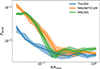 |
Fig. E.1. Radial profile of the minimum fractional temperature variation expected across one pixel from the smooth radial temperature gradient, δgrad. Shaded regions show the 16–84 percentile range across clusters. |
Appendix F: Voronoi temperature maps
To further investigate on the 2D temperature distribution in our simulations, we assessed the intrinsic azimuthal variations in the gas temperature profiles within each radial shell (Rasia et al. 2014; Lovisari et al. 2024). To this end, we generated Voronoi-tessellated images for each cluster, adopting a signal-to-noise ratio threshold of 30 per bin. We then extracted and fitted the X-ray spectrum in each Voronoi region within R500c, following the procedure outlined in Sect. 4. This yielded temperature maps based on Voronoi tessellation, which we used to characterise the azimuthal median temperature distribution at each radius. By comparing this to the results from direct X-ray spectral fitting, we could identify potential biases in the temperature measurement analogous to the analysis performed for surface brightness and gas density. The comparison is shown in Fig. F.1, where we plot the median ratio between the temperature profiles obtained from the azimuthal median of the Voronoi temperature maps in concentric annuli and those derived from direct X-ray spectral fitting. Shaded regions represent the 16th to 84th percentile spread of the distribution. In the innermost region within 0.1×R500c, the Voronoi-derived temperature profile is very close or systematically higher than the one obtained from spectral fitting in annuli. This is expected, as the annular spectral fit is particularly sensitive to bright, dense, and cool gas components that dominate the X-ray emission in the core, biasing the temperature low. In contrast, the azimuthal median computed from the Voronoi tessellation gives a more equal statistical weight to each spatial bin and is thus less affected by localised cool substructures. At such small radii the Voronoi maps do not contain enough resolution elements to provide a meaningful comparison. Since they are on average less massive, reaching a given signal to noise cut requires integrating larger regions. In the Voronoi temperature maps, we resolved the innermost 0.05×R500c with a median of 4 resolution elements, compared to 12 in MACSIS and 25 in The300. Between 0.1 and about 0.6×R500c, the trend reverses, with the Voronoi temperatures falling below the annular spectral fits. Similarly to the projection effects discussed for the SL and MW schemes, this may reflect a stronger sensitivity of the annular spectral fitting to high-emissivity, denser, and hotter gas that dominates the X-ray signal outside the core, where both the temperature and density profiles decrease. The Voronoi-based method, which downplays such emissivity-driven biases by construction, results in lower average temperatures. Beyond about 0.7–1×R500c, the scatter in the temperature ratio increases significantly. This is largely driven by the larger Voronoi cells required to maintain the desired signal-to-noise threshold in the outskirts, where the surface brightness is low. The reduced spatial resolution in these regions weakens the reliability of the comparison and introduces larger uncertainties in the azimuthal statistics.
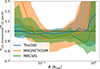 |
Fig. F.1. Comparison between the temperature profiles from X-ray spectral fitting and azimuthal median profiles obtained from Voronoi-tessellated temperature maps. |
To assess the robustness of our technique and rule out potential systematics, such as the limited spatial resolution of the Voronoi bins, low signal-to-noise ratios, or contamination from AGNs, we generated a dedicated high-exposure simulation (as described in Sect. 3.2) for a single cluster. This mock observation features a much deeper exposure time of 2 Ms and excludes AGN emission. We applied the same X-ray analysis pipeline and find that all thermodynamic profiles are in excellent agreement with those recovered from the standard 25 ks simulation, well within the uncertainties. We also produced the Voronoi-tessellated temperature maps for this deep mock observation. Given the computational expense of this process, which involves extracting and fitting spectra in 6002 Voronoi bins, we performed it for only one system. This served as a baseline for comparing the median temperature profile derived from the 2 Ms Voronoi map to that obtained from the standard 25 ks exposure. The full map extracted within R500c is shown in Fig. F.2. In the core of the 2 Ms observation, the signal-to-noise is high enough that the smallest Voronoi bins approach the native image pixel size of 2.5 arcsec. At the redshift of this system, z = 0.33, this corresponds to a physical scale of approximately 12 kpc. This is comparable to the effective resolution scale of the simulation. Therefore, the temperature structure probed by the smallest bins is not expected to be dominated by numerical resolution effects.
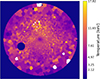 |
Fig. F.2. Voronoi-tessellated temperature map from the 2Ms XMM-Newton mock observation of the CL0030.1.115 cluster in The300 simulation. |
The median profiles extracted from the maps and the ones from X-ray spectral fitting in annular bins are reported in the upper panel of Fig. F.3, together with the input SL and MW ones. The bottom panel show the relative intrinsic scatter in the Voronoi median profiles extracted from the 25 ks and 2 Ms simulations. It is computed as the difference between the 84th and 16th percentile points of the distribution within each bin, divided by its median. This cluster has an R500c = 1491.5 kpc and is located at z = 0.33, so that R500c covers an angular scale of about 5.05 arcmin. We find good agreement between the results of the X-ray spectral fitting in annular bins of the 25 ks and 2 Ms simulations, with the latter being smoother and with lower uncertainties than the former by about one order of magnitude; the typical error bar is about 0.05 keV compared to 0.5 keV. This specific systems shows a small inconsistency with the SL temperature in the inner core within 0.8 arcmin, corresponding to about 0.15×R500c. However, the same trend is visible in both the 25 ks and 2 Ms simulations. Similarly to the spectral fit in radial bins, the median temperature profiles extracted from the Voronoi maps are also in agreement, with a discrepancy of about 6% at most, still well within the 1σ interval. We note that the reconstruction methods struggle to reproduce the input temperature in the core, even for deep (2 Ms) observations. This behaviour is consistent with the presence of strong multi-phase structure in the central regions. In these regions, the temperature distribution is broad and highly non-uniform, while the spectral fitting procedure assumes a single-temperature plasma. As a result, the recovered temperature represents an effective spectroscopic value that depends on the detailed weighting of different phases (e.g. Mazzotta et al. 2004), and does not necessarily exactly match the input expectation. This effect is intrinsic and cannot be mitigated by increasing the exposure time, as it arises from the physical structure of the gas rather than from statistical uncertainties. Finally, in both simulations we see an increasing trend of the intrinsic scatter as a function of radius, which is about 0.25 in the cluster core and get closer to 0.5 towards R500c. This is expected, as small regions in the core are more likely to include gas that is described well by a single temperature, whereas larger bins towards the outskirts are more likely to contain multi-phase gas, especially accounting for azimuthal variations in a single bin. The trend is smoother for the 2 Ms simulation, while the 25 ks one shows a big jump in the intrinsic scatter at about 2 arcmin, likely due to the low spatial resolution as a consequence of the large Voronoi bins to achieve the desired signal-to-noise ratio. Nonetheless, the median properties of the profiles are overall in agreement between the 25 ks and the 2 Ms simulations, suggesting that the residual discrepancies with the expected TSL are not primarily due to limited exposure depth, but rather to the intrinsic physics of the ICM.
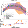 |
Fig. F.3. Temperature profiles extracted from the direct spectral fit and from the median of the Voronoi maps for the 25ks and 2Ms simulations of CL0030.1.115. |
F.1. Removing temperature fluctuations
We tested the impact of removing the most deviating regions from the 2D temperature distribution on the projected radial temperature profile. This is an attempt at replicating a similar strategy applied to CHEX-MATE by Lovisari et al. (2024) from the perspective of the simulation. The authors identified regions deviating more than 1σ from the ratio between the local 2D temperature map and the projected 1D profile. Such regions are likely associated with hot and cold gas clumps. We replicated the approach using 2D TSL maps and 1D TSL profiles, removing any systematic related to the temperature measurement by construction. In practice, for each pixel in the TSL maps we computed the quantity Si = 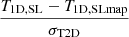 , where σT2D is the standard deviation of the temperature map at a given radius. We then selected and removed pixels with |Si|> 1 and recomputed the 1D median profile without outliers. The result is shown in Fig. F.4. We find that after removing outliers the temperature estimate increases by about 15-20%, which means that we are preferentially removing clumps of cold gas that are easier to detect. This matches the result obtained by Lovisari et al. (2024), who observed a similar trend with effects up to 10-20%.
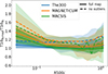 |
Fig. F.4. Comparison between the median of the 2D SL temperature maps and the 1D radial profile, before and after removing the most deviating regions. |
Appendix G: Mis-centring
We tested whether any inconsistencies in the reconstruction of gas density profiles in Sect. 5 is due to mis-centring. From the observer’s perspective, the profile is computed from the peak of the X-ray emission, while the input profiles use the position of the most bound particle, i.e. the deepest point of the potential well, as centre.
From the full population in each simulation, we sub-selected well-centred systems where the offset between the peak of the X-ray emission and the dark matter is ΔX < 0.007×R500c and studied the ratio between inferred and true density profiles. We respectively obtained 25, 15, and 15 well-centred systems in The300, Magneticum, and MACSIS. The result is shown in Fig. G.1. The ratio is basically unchanged in The300, which does not show significant inconsistencies even with the full sample. The issue is fully solved in MACSIS, where the ratio to true density is within 5% down to 0.06×R500c, whereas it crosses this threshold already at about 0.15×R500c for the full sample. For Magneticum the discrepancy decreases drastically, reaching a radius of about 0.08×R500c where the gas density is within 5% of the true value, compared to about 0.13×R500c for the full sample. Additional differences may be due to deviations from sphericity. In any case, the gas mass enclosed in such regions is a small fraction of the total one and does not impact the total gas mass reconstruction, as shown in Fig. A.3.
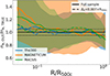 |
Fig. G.1. Ratio between reconstructed and true density profiles for all three simulations. The solid lines are for the full samples and the dashed ones for the well-centred objects only. The ΔX is the offset between the identified X-ray centre and the dark matter one. The dashed black lines denote the ±5% ratio. |
All Tables
Cosmological and numerical parameters describing the The300, Magneticum, and MACSIS simulations.
Best-fit beta model parameters of the gas density profiles in our simulations.
All Figures
|
Fig. 1. Mass and redshift distribution of the CHEX-MATE clusters compared to the twin-selected systems from The300, Magneticum, and MACSIS. The CHEX-MATE masses include the hydrostatic mass bias of 0.2. |
| In the text | |
|
Fig. 2. Example of a simulated XMM-Newton EPIC image for one cluster. The black lines denote the regions used for spectral extraction to measure its temperature profile. The red circle denotes R500c. |
| In the text | |
|
Fig. 3. Gas density profiles in our simulations. Top: Comparison between the measured (solid lines and shaded areas) and true (dashed lines) gas density profiles in different simulations (in various colours), using the NFW reconstruction. Bottom: Intrinsic dispersion in the selected population as a function of radius in units of dex. |
| In the text | |
|
Fig. 4. Ratio between the result of the X-ray spectral fitting and the input SL temperature profile. The profiles are also split between CC and NCC according to the ratio between the TSL profile measured at 0.05 and 0.2 R500c (TR). CC (NCC) have a ratio below (above) 0.8. |
| In the text | |
|
Fig. 5. Gas temperature profiles. Each column corresponds to one simulation: The300 (left), Magneticum (centre), and MACSIS (right). The colours denote the three reconstruction methods. The smaller lower panels show the ratio between the reconstructed 2D and deprojected 3D profiles. |
| In the text | |
|
Fig. 6. Ratio between the SL and MW temperature profiles in different simulations. |
| In the text | |
|
Fig. 7. Comparison between the distribution of the local SL temperature fluctuations in 2D maps within different apertures for different simulations. TLOC is the 1D radial profile at the position of each pixel in the map. |
| In the text | |
|
Fig. 8. Ratio between the SL and MW temperature profiles as a function of the standard deviation of the SL temperature fluctuations. The points are colour-coded by the median of the fluctuation distributions. |
| In the text | |
|
Fig. A.1. Density profile reconstruction of CL0017.1.119 from The300 simulation. |
| In the text | |
|
Fig. A.2. Deprojected 3D gas density profiles. Each column corresponds to one simulation: The300 (left), Magneticum (centre), and MACSIS (right). The colours denote the three reconstruction methods. The smaller central (bottom) panels show the ratio between the median Voronoi (the standard mean) profile and the true input one. |
| In the text | |
|
Fig. A.3. Comparison between the measured and true gas mass within R500c. The masses were inferred from the Voronoi-tessellated images. The dashed coloured lines denote the best linear fit to each simulation. |
| In the text | |
|
Fig. B.1. Ratio between the reconstructed 2D temperature profile with NFW, NP, and FM models to the result of the X-ray spectral fitting in MACSIS. |
| In the text | |
|
Fig. B.2. Comparison between the SL temperature estimated within R500c and that estimated from the modelled temperature profile within the true R500c. |
| In the text | |
|
Fig. B.3. Corner plot with the marginalised 1D posterior distribution of the parameters describing the ratio between the SL and MW temperature as a function of median and width of the temperature fluctuation distribution. |
| In the text | |
|
Fig. B.4. Deprojected 3D electron pressure profiles. Each column corresponds to one simulation: The300 (left), Magneticum (centre), and MACSIS (right). The colours denote the three reconstruction methods. The smaller central (bottom) panels show the ratio between the median Voronoi (the standard mean) profile and the true input one. |
| In the text | |
|
Fig. B.5. Deprojected 3D gas entropy profiles. Each column corresponds to one simulation: The300 (left), Magneticum (centre), and MACSIS (right). The colours denote the three reconstruction methods. The smaller central (bottom) panels show the ratio between the median Voronoi (the standard mean) profile and the true input one. |
| In the text | |
|
Fig. C.1. Equivalent to Fig. 1, with the addition of two sub-selections designed to test selection effects related to mass and redshift. |
| In the text | |
|
Fig. C.2. Equivalent to Fig. A.2, relative to two subsamples selected to test the impact of mass and redshift on density profiles. |
| In the text | |
|
Fig. D.1. Spherical isothermal toy model of the gas temperature profile, including its projections along the line of sight assuming the SL and MW temperature schemes. |
| In the text | |
|
Fig. E.1. Radial profile of the minimum fractional temperature variation expected across one pixel from the smooth radial temperature gradient, δgrad. Shaded regions show the 16–84 percentile range across clusters. |
| In the text | |
|
Fig. F.1. Comparison between the temperature profiles from X-ray spectral fitting and azimuthal median profiles obtained from Voronoi-tessellated temperature maps. |
| In the text | |
|
Fig. F.2. Voronoi-tessellated temperature map from the 2Ms XMM-Newton mock observation of the CL0030.1.115 cluster in The300 simulation. |
| In the text | |
|
Fig. F.3. Temperature profiles extracted from the direct spectral fit and from the median of the Voronoi maps for the 25ks and 2Ms simulations of CL0030.1.115. |
| In the text | |
|
Fig. F.4. Comparison between the median of the 2D SL temperature maps and the 1D radial profile, before and after removing the most deviating regions. |
| In the text | |
|
Fig. G.1. Ratio between reconstructed and true density profiles for all three simulations. The solid lines are for the full samples and the dashed ones for the well-centred objects only. The ΔX is the offset between the identified X-ray centre and the dark matter one. The dashed black lines denote the ±5% ratio. |
| In the text | |
Current usage metrics show cumulative count of Article Views (full-text article views including HTML views, PDF and ePub downloads, according to the available data) and Abstracts Views on Vision4Press platform.
Data correspond to usage on the plateform after 2015. The current usage metrics is available 48-96 hours after online publication and is updated daily on week days.
Initial download of the metrics may take a while.