


| Issue |
A&A
Volume 711, July 2026
|
|
|---|---|---|
| Article Number | A232 | |
| Number of page(s) | 17 | |
| Section | Galactic structure, stellar clusters and populations | |
| DOI | https://doi.org/10.1051/0004-6361/202558263 | |
| Published online | 17 July 2026 | |
Extinction law and stellar mass in the nuclear bulge from kinematically selected red clump stars
1
Instituto de Astrofísica, Pontificia Universidad Católica de Chile,
Av. Vicuña Mackenna
4860,
Santiago,
Chile
2
European Southern Observatory,
Karl Schwarzschild-Straße 2,
85748
Garching bei München,
Germany
3
Excellence Cluster ORIGINS,
Boltzmann-Straße 2,
85748
Garching bei München,
Germany
4
Departamento de Física, Universidad de Santiago de Chile,
Av. Victor Jara
3659,
Santiago,
Chile
5
Center for Interdisciplinary Research in Astrophysics and Space Exploration (CIRAS), Universidad de Santiago de Chile,
Santiago,
Chile
6
European Southern Observatory,
Alonso de Córdova 3107, Vitacura,
Casilla
19001,
Santiago,
Chile
7
Max Planck Institute for Astronomy,
69117
Heidelberg,
Germany
8
Fakultät für Physik und Astronomie, Universität Heidelberg,
Im Neuenheimer Feld 226,
69120
Heidelberg,
Germany
9
Instituto de Astrofísica de Canarias,
La Laguna,
Tenerife,
Spain
10
Departamento de Astrofísica, Universidad de La Laguna,
Tenerife,
Spain
11
INAF – Osservatorio Astronomico di Capodimonte,
salita Moiariello 16,
80131
Naples,
Italy
12
Université Côte d’Azur, Observatoire de la Côte d’Azur,
CNRS, Laboratoire Lagrange, Blvd de l’Observatoire,
06304
Nice,
France
13
International Gemini Observatory/NSF NOIRLab,
Casilla 603,
La Serena,
Chile
14
Aryabhatta Research Institute of Observational Sciences,
Manora Peak,
Nainital
263002,
India
15
Division of Astrophysics, Department of Physics, Lund University,
Box 118,
22100
Lund,
Sweden
16
INAF – Osservatorio Astronomico di Padova,
Vicolo dell’Osservatorio 5,
35122
Padova,
Italy
★ Corresponding author: This email address is being protected from spambots. You need JavaScript enabled to view it.
Received:
25
November
2025
Accepted:
29
April
2026
Abstract
Context. The nuclear bulge of the Milky Way harbors stellar populations that provide crucial insights into galaxy formation processes and serve as a nearby analog for understanding bulge formation in external galaxies. However, detailed studies of this region are severely hampered by extreme and highly variable interstellar extinction, which obscures the intrinsic stellar properties and impedes accurate stellar mass determinations.
Aims. Our goal is to measure the extinction law toward the nuclear bulge and to estimate its stellar density.
Methods. We developed a method for determining the extinction law toward the nuclear bulge by kinematically selecting red clump stars that belong to this region. We created a reddening map with a high spatial resolution and computed stellar mass with completeness-corrected red clump star counts, scaled from empirical measurements.
Results. We find a total-to-selective extinction ratio of AK/EH-K = 1.259 ± 0.074 and an extinction ratio of AH/AK = 1.794 ± 0.046, which are consistent with previous works. The reddending map with the high spatial resolution shows clear filamentary structures and a gradient in the extinction over the giant molecular cloud G0.253+0.016 (i.e., the Brick). From the star counts, we measured a stellar mass of 12.2 ± 2.6 × 10⁸ M⊙ for the nuclear bulge, in agreement with other mass estimates.
Key words: Hertzsprung–Russell and C–M diagrams / dust, extinction / Galaxy: center / Galaxy: stellar content / infrared: stars
© The Authors 2026
 Open Access article, published by EDP Sciences, under the terms of the Creative Commons Attribution License (https://creativecommons.org/licenses/by/4.0), which permits unrestricted use, distribution, and reproduction in any medium, provided the original work is properly cited.
This article is published in open access under the Subscribe to Open model. This email address is being protected from spambots. You need JavaScript enabled to view it. to support open access publication.
1 Introduction
The Milky Way (MW) is a barred spiral galaxy, with the Sun located within the disk at ~8.2 kpc from its center (GRAVITY Collaboration 2019, 2022). The region within ~3 kpc from the center is known as the bulge. It has a stellar mass of ~ 2 × 10¹⁰ M⊙ (e.g. Portail et al. 2015; Valenti et al. 2016; Simion et al. 2017), which represents about one-third of the total stellar mass of the Galaxy. The MW bulge is mainly composed of stars over 10 Gyr (e.g. Zoccali et al. 2003; Renzini et al. 2018), meaning that it is the first massive structure to have formed in the MW. Therefore, it holds vital information about its mass assembly history that we must understand to know how and when the bulge formed (see Zoccali & Valenti 2026, for a review).
It is still debated whether all the stars in the MW bulge were formed in situ or if some fraction of them resulted from the accretion of external stellar systems. Notably, within the bulge lies a small (~200 pc radius) star-forming region near the Galactic center (GC), called the nuclear bulge (NB, Mezger et al. 1996). This region is formed of gas-phase structures and stars; the former is known as the central molecular zone (CMZ), and the latter contains several stellar substructures, such as young massive star clusters (i.e., Arches and Quintuplet), a nuclear star cluster (NSC), and an extended component usually referred to as the nuclear stellar disk (NSD; all references bellow, from Schönrich et al. 2015). Hereafter, we use the term NB to refer to the entire region, although we focus on the stellar content. We prefer to avoid using the term NSD, as the detailed morphology and kinematic structure of this region remain under active investigation. Evidence exists for additional components, including an inner bar (Alard 2001; Rodriguez-Fernandez & Combes 2008), and questions persist regarding the kinematic properties and whether a distinct disk-like component can be identified unambiguously (see Sect. 6 in Zoccali et al. 2024) (for a comprehensive review of the Galactic NSD and those in external galaxies, see Schultheis et al. 2025).
Recent simulations indicate that these nuclear structures formed through secular evolution after the bulge formed a bar. The bar changes the gravitational potential, which funnels gas along the main bar axis. When the gas reaches the center, star formation is triggered, forming nuclear disks, rings, or clusters (see e.g. Fragkoudi et al. 2016; Sormani et al. 2020b; Tress et al. 2020). Some of the stars within the NB might indeed have been formed from the gas from the CMZ (Sormani et al. 2020b; Schultheis et al. 2021). Therefore, if we can measure the ages of the first stars that compose the NB, we can estimate an epoch for the formation of the bar of the Milky Way (e.g. Baba & Kawata 2020; Bittner et al. 2020; de Sá-Freitas et al. 2023, 2025). In turn, it is important to date the MW bar because it constrains Galactic formation models and cosmological simulations.
The nuclear structures observed in the MW have also been detected in other galaxies (e.g., Gadotti et al. 2019; Schultheis et al. 2025), and the NB can help us to understand star formation in distant galaxies. The physical conditions of the gas structures within the CMZ resemble those of high-redshift galaxies in terms of temperature, density, velocity dispersion, and magnetic fields. Unlike those distant galaxies, where individual structures cannot be resolved, the CMZ lies in our own cosmic backyard, allowing us to study star formation processes in unprecedented detail under these physical conditions. For this reason, Kruijssen & Longmore (2013) referred to the CMZ as a “high-redshift analog” star-forming region.
Furthermore, the CMZ presents a unique opportunity to understand scaling relations. One of these relations is known as the Schmidt–Kennicutt (SK) law (Schmidt 1959; Kennicutt 1998), which correlates the star formation rate (SFR) surface density with the total gas surface density. Although this relation holds for many physical scales, that is, from nearby star-forming regions to distant starburst galaxies, Longmore et al. (2013) found that the CMZ lies one order of magnitude below the expected value of SFR density given the SK law. This might indicate that star formation depends on environmental factors other than the cloud density (see e.g. Henshaw et al. 2023, and references therein). Solving this puzzle might enhance our understanding of the details of star formation processes and their interactions with the environment.
Because the NB is relevant for all these different aspects of astrophysics, it is crucial to study the stellar populations that compose it in depth. However, any attempt to observe the NB must have a high spatial resolution because the crowding levels toward this particular direction in the sky are high. Unfortunately, a high spatial resolution is often coupled with a small field of view, and deep space-based observations are therefore only available for some sparse fields (e.g. Hosek et al. 2022; Schödel et al. 2023). Because this region has a high surface density of stars and extreme extinction, optical wavelengths are virtually blind to the stellar populations in the NB. To solve this, we must use high spatial resolution near-infrared (NIR) photometry, often coupled with adaptive optics (see e.g. Stolte et al. 2015, analyzing the Arches and Quintuplet clusters). All these difficulties have deterred comprehensive and homogeneous observational campaigns in the NB region.
Nevertheless, in recent years, the GALACTICNUCLEUS project (GNC, Nogueras-Lara et al. 2019) overcame the aforementioned observational difficulties and studied the NB region in detail. For the first time, a dedicated observational campaign produced deep NIR catalogs for J, H, and KS filters, extinction ratios, reddening map, and star formation history (SFH) estimations for stars in the NB over an area of 0.3 deg2 Nogueras-Lara et al. (2019, 2020, 2020, 2021a). They achieved all this by using the HAWK-I NIR imager (Pirard et al. 2004; Casali et al. 2006; Kissler-Patig et al. 2008; Siebenmorgen et al. 2011) located at the Very Large Telescope (VLT) UT-4 telescope in Cerro Paranal, using the speckle holography photometry technique described in Schödel et al. (2013).
Overlapping with the GNC survey, a similar archival dataset was obtained using the HAWK-I imager (ID 0103.B–0262(A), PI: Zoccali, hereafter referred to as NB field, NBF). Unlike the observation strategy adopted by GNC, we did not use speckle holography, and obtained shallow and deep observations in five fields1 centered at b = 0° between |l| < 0.37°, covering approximately 320 arcmin2. The two datasets provide an opportunity for an independent verification of the scientific results in the NB. The spatial coverage of both datasets is shown in the top panel of Fig. 1.
One key aspect that is critical for all the science in the NB is the characterization of the extinction and reddening toward this particular direction of the MW. Previous studies, including GNC survey, have shown that the extinction values are severe and can be as high as AV ≥ 30 mag and AKs ≥ 2.5 mag (e.g. Nishiyama et al. 2006; Schödel et al. 2010; Nogueras-Lara et al. 2020). Moreover, there is evidence of a wavelength dependence in the extinction law toward the NB (Nogueras-Lara et al. 2020), which makes it even more critical to a deep understanding of the effect of the dust on stellar observations. Current reddening maps available in this area were produced using the red clump (RC) method (Nishiyama et al. 2006), which uses this feature in the observed color–magnitude diagrams (CMDs) to trace stellar structures composed of metal-rich core helium-burning stars (see Girardi 2016, for comprehensive review). RC stars have been used to trace Galactic structures, such as the Galactic bar (e.g. Stanek et al. 1994, 1997; Wegg & Gerhard 2013; Simion et al. 2017; Gonzalez et al. 2018), and also to study the Galactic extinction law (e.g. Nishiyama et al. 2006, 2009; Alonso-García et al. 2015, 2017; Sanders et al. 2022). Even more, accurate RC star counts can be used to compute the stellar mass content: Valenti et al. (2016) measured the stellar content of the MW Bulge by using RC stars with an empirical approach, and Simion et al. (2017) did the same assuming a Chabrier initial mass function (IMF). We discuss the latter method in Sect. 4.
We use the RC stars as extinction and structure tracers by assuming that the slope in the observed CMDs does not represent the reddening law (as pointed out, e.g., by Nishiyama et al. 2006; Nogueras-Lara et al. 2019), but is the combination of extinction and distance spread along the line of sight (LOS), with a different extinction at each layer. To assess this, we used kinematics of RC stars in the NB to derive a new extinction law. This method relies on the fact that stars on the near side of the NSD are expected to rotate in a direction opposite to that of the far side. From there, we constructed a reddening map with a high spatial resolution. Finally, we used completeness-corrected RC star counts to estimate the stellar content of the NB.
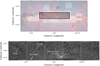 |
Fig. 1 Top: image of the NB of the MW from the GLIMPSE360 survey (Whitney et al. 2011) from the Spitzer Space Telescope. The 4.5 μm image is shown in red and the 3.6 μm is shown in blue. The black line surrounding the dark shaded area indicates the footprint of our dataset, as shown in the bottom panel. The dotted gray line encompassing the white shaded area depicts the GNC survey area. Bottom: five HAWK-I pointings in KS filter, covering the innermost part of the NB. Some relevant structures are indicated with arrows. The vertical white lines show the overlapping regions between the adjoint HAWK-I pointings. |
2 Data
2.1 Image reduction and processing
We analyzed H and KS observations obtained with HAWK-I NIR imager at VLT-UT4 (Yepun Telescope) at ESO Paranal Observatory. HAWK-I has a field of view (FoV) of 7.5× 7.5 arcmin, with a spatial resolution of 0.106 arcsec/pix. The dataset comprises five fields observed within program ID 0103.B-0262(A), between July and September 2019. The seeing during the observations was 0.7 arcsec on average, but the GRound layer Adaptive optics system Assisted by Laser (GRAAL) system (Arsenault et al. 2008; Paufique et al. 2010) improved the point spread function full width at half maximum (PSF FWHM) to 0.4 arcsec for the H band and 0.3 arcsec for KS. The dithering pattern of the observations was designed to homogeneously cover the 15 arcsec gap between the four detectors and to improve the sky subtraction.
The raw data were processed using the HAWK-I pipeline within the Reflex workflow2. To account for instrumental signatures, the pipeline first generates a set of calibration products, including a combined dark frame (with the associated bad-pixel map), a master flat field to correct for pixel-to-pixel sensitivity variation, and estimates of the readout noise, gain, and covariance for each HAWK-I detector. These calibrations are applied to each dithered science exposure, after which the sky background (derived from a median combination of the dithered images) is subtracted. Finally, the pipeline realigns the corrected science frames for each filter and combines them into a stacked image. More details about the pipeline procedure and algorithms can be found on the ESO pipeline web page3.
The observing strategy consisted of long- and short-exposure images to detect fainter stars in the former and recover brighter stars in the latter. For the long KS filter, one stacked image was produced from eight individual images with exposures of 10 s with two sub-integrations, giving a total exposure time of 160 s. For the long H-band, the stacked image was produced from 16 individual 10 s exposures with three sub-integrations for a total exposure time of 480 s. On the other hand, all the short exposure images for H and KS filters were produced from five individual images, 2 s long with one sub-integration, resulting in a total exposure time of 10 s. Field NBF058 has one additional stacked image of 180 s, produced from six individual 10s images with three sub-integrations. Table A.1 summarizes the data we used.
The complete mosaic of all five fields for KS images is shown in the bottom panel of Fig. 1. Some relevant structures can be spotted just by visual inspection, such as the NSC (central tile) and two young massive clusters: Arches and Quintuplet (second tile from the left), and the giant molecular cloud G0.253+0.016 (from now on, the Brick, in the first tile on the left). The former belongs to the tile NBF054, which was presented and discussed in Zoccali et al. (2021).
2.2 PSF photometry
We performed PSF profile fitting using the softwares DAOPHOT (Stetson 1987), ALLSTAR, and ALLFRAME (Stetson 1994) on a total of 28 H and KS images (Nobs in Table A.1)4. We worked on each of the four HAWK-I detectors (i.e., chips) individually. As a first step, we performed Find and aperture Photometry on each chip, with standard parameters (e.g., detector gain, saturation, and FWHM). We then drew 200 isolated stars for each chip, which we visually inspected to select the 30–50 best to create a first PSF model. As a second iteration, we subtracted all the neighbors from these stars and created a new, cleaner model, which was used to perform the ALLSTAR photometry. The output catalogs were registered using the DAOMATCH routine and were stacked using MONTAGE2. A new complete PSF photometry was performed on this stacked image using the PSF model from a long exposure H band. This catalog was used as a master star list to give as input to ALLFRAME, which produced the final photometry we analyzed here.
2.3 Photometric calibration
Our goal was to calibrate the HAWK-I photometry to the 2MASS system (Skrutskie et al. 2006). However, the stars in common between NBFs and 2MASS are either saturated in HAWK-I data or are very faint in 2MASS. The difference in spatial resolution also makes a direct cross-match difficult. Therefore, we used the Vista Variable in the Via Lactea Survey (VVV, Minniti et al. 2010) as an intermediary between the NBF and 2MASS.
First, we calibrated the VVV/VVVX PSF photometry (Contraras Ramos, private communication) to 2MASS following a color-dependent transformation. The color terms (CTs) between 2MASS and VVV are, in fact, non-negligible but small: CTH = 0.048 ± 0.004 and CTKs = 0.026 ± 0.007, in the H and KS bands, respectively. The zeropoints (ZP) were found by cross-matching the stars of 2MASS and VVV in the overlapping region with the NBFs, and we report them in Table B.1. As a second step, we used the calibrated VVV catalog as a reference to calibrate the NBF photometry using a color-dependent photometric transformation. The CT and a ZP were applied to each chip when the obtained values were not consistent with zero within the uncertainties. We provide the technical details of the calibration in Appendix B.
After calibrating each individual NBF chip, we merged the 2MASS-calibrated NBF photometry for individual HAWK-I chips into a single catalog, with 974 361 stars. In the overlapping regions of NBFs, the quoted magnitude is the mean of the measured magnitude on each chip, and the errors are added in quadrature. Hereafter, the calibrated NBFs KS magnitude are labeled K for simplicity.
The final CMD is shown in Fig. 2. Some distinctive features from foreground stars are present, such as the disk main-sequence (MS) stars at color H-K ∼ 0.2, and the disk RC stars. Most of the stars are heavily extincted. The RC stars are spread along a line from H-K ∼ 1.0 to ∼3.5, which is often used to constrain the extinction (see section 3 for a further discussion). Moreover, a prominent asymptotic giant branch (AGB) bump is observed above the RC. The red giant branch (RGB) and AGB sequences merge above the AGB bump, which is expected for these NIR filters.
In the left part of the CMD, we show typical errors for each bin of K magnitude. For the magnitude range in which artificial stars were injected (see Sect. 4.1), the black error bars represent the mean difference between injected and recovered magnitudes and colors within each K bin, as derived from the artificial stars tests (ATSs). For the remaining CMD region in which no artificial stars were injected, we report the typical photometric uncertainty from ALLFRAME, shown in red. In both cases, the color uncertainty was computed by adding the H and K errors in quadrature. As expected, the uncertainties increase toward fainter magnitudes, while the brightest bins show higher uncertainties because they lie close to the saturation limit.
Sampling stars down to K ∼ 20.5 ± 0.3, the derived K, H-K CMD is one of the deepest obtained for the NB region from ground-based facilities. For comparison, the GNC reaches a magnitude limit of K ∼ 18.5, which is discussed further in Sect. 4.1. Other differences in the photometry of the GNC project are beyond the scope for this study.
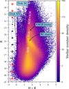 |
Fig. 2 Color–magnitude diagram of all the NBFs colored by density. The key observed features are labeled. The color bar shows the stellar number density, and the color scale is on a logarithmic scale to enhance the visibility of other features that are less populated than the RC. The typical photometric errors are shown on the left. The red dots show the photometric errors reported by DAOPHOT/ALLFRAME, and the black error bars were computed with the difference between the input and output magnitudes from the artificial star tests (see Sect. 4.1). |
3 Kinematic determination of the extinction law
The extinction law toward the MW bulge has been derived by means of different techniques. Nishiyama et al. (2006) developed the RC method based on the fact that the intrinsic luminosity of RC stars changes little with metallicity and age (e.g., Girardi 2016, for a comprehensive review); thus, they can be used as standard candles. The authors argued that if an RC is affected by different levels of extinction, it would change its position in the CMD along the reddening vector, with a slope equal to the ratio of the total to selective extinction Rλ = Aλ/Eλ′-λ. When we observe the CMD of the NBFs, which has severe differential extinction (see Fig. 2), the RC is indeed spread along a line toward redder and fainter magnitudes. However, the underlying assumption is that the RC stars used for this derivation are all at the same distance, which is not necessarily true. While it is true that the NSD diameter (~400 pc) is small compared to its mean distance, it is also true that foreground contamination from the disk and the bulge, at b = 0°, is non-negligible, and it might produce structures in the RC that modify its observed slope.
In the NB region, RC stars have also been used to study the extinction law. Sanders et al. (2022) combined data from VIRAC2 (Smith et al. 2025), GLIMPSE (Whitney et al. 2011), and the unWISE catalog (Schlafly et al. 2019) to produce reddening maps for the inner regions of the Milky Way by combining the RC method with the Rayleigh Jeans color-excess method (RJCE). In order for their method to work, they assumed that the distribution of RC stars peaks at the distance of the GC (GRAVITY Collaboration 2022). Furthermore, Nogueras-Lara et al. (2020) used the slope of the RC to measure the extinction law toward different regions in the GALACTICNUCLEUS survey, and later, Nogueras-Lara et al. (2021a) used the derived values to create reddening maps using a two-layer approach.
To address the dust toward the NB, we developed a novel method to determine the extinction law based on the kinematics of the observed RC stars. We know that due to the rotation of the NB, stars in front of the NB must have different longitude proper motion (µl) from those behind the GC. Along with the assumption that the peak of RC density is located at the GC distance, we also assumed that nonlinear effects in the extinction are negligible. Thus, we measured where the position of the RC was at low but nonzero extinction and compared it with the peak of the RC star distribution around the GC.
To implement this, we followed these steps: first, we extracted bona fide RC stars from the NBFs. Then, we determined the position of the RC with negligible extinction (referred to as the anchor RC). Finally, we determined the RC stars near the GC using their kinematics (referred to as kinematical center; KC0).
3.1 RC selection
To select bona fide RC stars, we defined a parallelogram around this feature. To derive the slope of the upper and lower sides, we adopted the method called unsharp-masking technique (see De Marchi et al. 2016; Hosek et al. 2018). This method enhances the contrast in CMDs, making distinctive, high-density features such as the RC more prominent.
First, we created a Hess diagram binned by 0.1 in K and 0.06 mag in H-K, as shown in the left panel of Fig. 3. Then, we convolved the diagram with a 2D Gaussian profile of σ = 0.05 to incorporate internal observational errors into the data. Afterward, we applied a second convolution with a wider Gaussian profile of σ = 0.2 to create the mask that enhances high-frequency features. Finally, we subtracted the mask from the original Hess diagram and obtained the diagram on the right of Fig. 3. As suggested in De Marchi et al. (2016), we explored several values of σ to create the mask, from 0.15 to 0.35, and we found no significant difference in the results.
We applied a linear regression to compute the slope and the intercept that describe the peak RC stars. The resulting linear function is K = 1.456(H-K) + 12.463. In order to derive the extinction law, we defined the stars between ±0.7 mag from this line as the RC sample.
The color limits of RC stars in the NB change dramatically due to extinction from one region to the next. This is illustrated in Fig. 4, where we show the CMD of three regions 50" × 50" wide. For this reason, we selected by visual inspection a blue and a red RC color cut in each spatial bin. The blue cut is usually evident, whereas the red cut is more ambiguous and therefore arbitrary, because the red side of the distribution falls off more smoothly. Nonetheless, the exact location of this cutoff does not affect the results presented here because we removed ~10% of the stars, only in the red tail. This did not affect the determination of the kinematic center (Sect. 3.3) or the stellar density (Sect. 4).
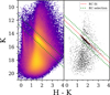 |
Fig. 3 Red clump position using the unsharp-masking technique. The dotted green line shows the upper and lower limits of the RC selection. Left: Hess diagram of our complete catalog. A logarithmic stretch was applied in a range from 1 to 2000. Right: Hess diagram after applying the unsharp-masking technique. |
3.2 Anchor RC position
The next step was to determine what the observational position of the RC would be if the bulk of the stars were located at the GC distance and the extinction were negligible. We decided to use the positions of three different low-extinction fields in the MW bulge to compute this point: Stanek ((l,b) = (0.25°, −2.15°)), SWEEPS ((l,b) = (1.25°, −2.65°)), and Baade’s Window (BW; (l,b) = (1.04°, −3.88°)). To compute the position of the RC in these regions, we used VVV+VVVX PSF photometry from the catalog of Contreras Ramos (private communication) and selected a circular area with a radius of 0.5° around the central coordinates of each field. For consistency, we calibrated the photometry to 2MASS using the same procedure as described in Sect. 2. Then, we selected RC stars with 10 ≤ K ≤ 14. In this magnitude range, we fitted the luminosity function (LF) with an exponential function and a Gaussian using the least-squares minimization technique. We determined the position of the RC as the mean of the Gaussian. For the color in H-K, we employed a Gaussian mixture model to fit the data within the same magnitude range. We verified that the position of the RC in BW was consistent with that reported in Zoccali et al. (2021), and we found no significant offset in color or magnitude.
We applied this method to the three fields. The positions of the RCs are shown in the inset panel A of Fig. 5. The average is represented with a golden star, which is (H-K, K) = (0.192, 13.135). The difference in position of each RC along this window is small, less than 0.05 mag in color and magnitude.
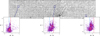 |
Fig. 4 Same image as in the bottom panel of Fig. 1, showing examples of CMD in three different 50″ × 50″ regions. In all insets, the visually selected bluer and redder ends of each RC are shown as vertical blue and dashed red lines, respectively. The left inset shows a thin well-defined RGB with a prominent RC in H-K ~ 1. The middle inset shows two RC features: one feature with a low extinction at H-K ~ 1, and another feature with a high extinction centered at H-K ~ 2. Between these two RCs, there is a gap without stars. The right inset shows a spread RC. |
3.3 Kinematical center in the CMD
To determine the KC0, we relied on the PM from the same PSF VVV+VVVX catalog. We performed a cross-match with VVV and assigned these PM to all our NBF stars, which are calibrated to the Gaia reference system (μgrs). To determine the kinematical center, we referred the PM with respect to Sgr A* (μl,μb) = (—6.41, −0.219) mas yr−1 (Reid & Brunthaler 2020).
Panel C of Fig. 5 shows the CMD colored by the mean PM inside each bin. We detect a coherent change in the rotation of stars at color H-K - 1.9. To determine this color, we used panel E from Fig. 5, where we correlated the longitudinal PM with the color only for our RC stars that matched the VVV. The gray squares in the background show the density of points. There is a clear trend with the color to change the direction of rotation. To model the rotation, we employed a running median algorithm with a bin size of 0.1 mag and fitted a third-degree polynomial to all the medians. The color at which the rotation changes direction is where the fit reaches zero, and this occurs at (H-K)KC0 = 1.96.
We then determined the magnitude of the peak RC stars around the kinematical center. To do this, we selected all RC stars within 0.1 mag around (H-K)KC0 and determined the maximum on their K LF. We used a linear kernel density estimator (KDE) from sktlearn to determine the maximum in the LF and found a value of Kpeak = 15.38. This procedure is shown in panel D of Fig. 5.
Finally, we used the location of the KC0 in all fields (i.e., the purple cross with white edges in Fig. 5), with the position of the anchor RC (i.e., the golden star in Fig. 5, see Sect. 3.2) to trace the extinction law. In panels A and B of Fig. 5, the derived extinction law is shown as a dashed gold line. The total-to-selective extinction ratio and the H and K extinction ratios are
 (1)
(1)
If our method is correct, then we might measure a different KC0 in each of the five NBFs because the GC might be seen behind different amounts of clouds, along different lines of sight, but all the KC0 should align, within the errors, along the same extinction vector derived above. We verified our results by measuring the total-to-selective extinction ratio again. This time, we performed a least-squares fit using all NBFs points (i.e., squares in Fig. 5, panel B), and forced the fit to pass through the RC anchor position (i.e., the golden star in Fig. 5, panels A and B). Since the RC locus is expected to move along the extinction vector as the extinction varies (Nishiyama et al. 2006, 2009), it is normal that some KC0s in some fields are less extincted than others. The less extincted field is NBF070, toward the LOS, with less dust in the CMZ. Using this method, we obtained a total-to-selective extinction ratio of AK/EH-K = 1.265 and an extinction ratio of AH/AK = 1.791, which are consistent with the values computed using all the fields.
We estimated the uncertainty in the total-to-selective extinction ratio by resampling the KC0 positions of each individual NBF field from normal distributions and repeating the linear fit 20 000 times, always forcing it to go through the RC anchor position. We computed the uncertainty as the standard deviation of the distribution of total-to-selective ratios. We considered homoscedastic errors of 0.1 mag in color, corresponding to the bin width used to determine the kinematic center for each field. For the K magnitude, we used 0.25 mag, which is the approximate width of the K LF on each field. To estimate the uncertainty in the absolute extinction ratios, we analytically propagated the errors.
All the individual KC0 and the one using all fields are shown in panel B of Fig. 5. As observed, each individual field is scattered around the extinction law derived using all fields, which might suggest a dependence of the extinction law variation on the LOS. These spatial variations were observed in the NIR regime in previous works, but on larger scales (e.g. Nishiyama et al. 2006; Alonso-García et al. 2017). Overall, our derived extinction ratios are consistent with previous measurements in the literature toward this region of the MW, as discussed in Sect. 5.2.
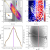 |
Fig. 5 Determination of the extinction law. All the panels and inset share the same color-coding and line style. The best fit for the RC (computed in Sect. 3.1) is shown with a dashed white line; the derived extinction law is shown as a dotted gold line; the color at which RC stars change the direction of rotation with respect to Sgr A* is represented with a solid red line and a shadowed gray area; and the K magnitude at which the maximum of the RC is at the color of transition in kinematics is shown with a solid purple line. A: zoom on the region near the RC anchor. The crosses show the positions of the RC in low-extinction windows without uncertainties. The gold star with black edges represents the anchor RC position, which is the average of the RC in the windows. B: color–magnitude diagram showing the RC selection colored by density. The gray dots represent all the stars not included in the RC selection. C: color–magnitude diagram of NBF stars cross-matched with VVV stars. Each bin is colored by the mean PM along the Galactic latitude with respect to Sgr A*. The contours show the density of RC selection stars. D: K LF within the 0.1 mag around (H-K)KC0. The orange histogram represents the LF, and the solid black line represents the KDE fit. E: longitudinal proper motions with respect to the proper motion of Sgr A* as a function of the observed color. The gray background represents the density of stars in this space. A logarithmic stretch was applied for better visualization. The black dots show the median of each 0.1 mag in color. The solid black line represents the best fit for the medians. The horizontal dashed black line shows where the proper motion with respect to the Sgr A* changes its rotation direction. |
3.4 High-resolution reddening map
With this total-to-selective extinction ratio and our selection of RC stars, we constructed a reddening map for the region. First, we binned our region with a bin size of 4.5″ × 4.5″. With these bins, we had a mean of five stars RC stars per bin. For each RC star, we computed their reddening assuming a reference color of (H-K)0 = 0.1, which is the observed intrinsic color in the same region (Nogueras-Lara et al. 2021a). We averaged the extinction of the RC stars within each spatial bin.
This initial map has some bins with no stars. To fill them, we reconstructed the map with the astrofix package (Zhang & Brandt 2021). In short, this package interpolates images using a Gaussian process regression to fix bad pixels. When applied to our reddening map, it predicts the extinction value for each bin5.
We are confident in applying this method to our map because only ~5% was fixed using this method. Some bins without RC stars might be due to strong interstellar extinction. If this were the case, the amount of extinction in the interpolated bins must be higher than in their surroundings. Therefore, these bins should be considered as a lower limit for the extinction.
Finally, we assigned an extinction value to each star in the NBFs interpolating the binned reddening map using a radial basis function (RBF) interpolator implemented in scipy (Virtanen et al. 2020). We used a thin-plate spline kernel, with a first-degree polynomial added to reproduce the linear trends across the field. We interpolated using the ten nearest bin centers to each query point, ensuring that the assigned extinction value of each star reflected the local structure of the map and not a global fit. The result of this map is shown in panel A of Fig. 6. In the same figure, we show the reddening maps from Sanders et al. (2022), Zelakiewicz et al. (2025), and Surot et al. (2020) in panels B, C, and D, respectively.
Some distinctive features are evident in our map. First, there is a clear gradient in the reddening on top of the Brick ((l, b) ~ (0.25°, 0.02°)). The location of the Brick is shown in Fig. 6 as dashed white lines, and the zoom-in of our reddening map on top of the Brick is shown in Fig. 7. The northern region of the Brick is less extinct than the southern part. This is not an artifact: the gradient is also evident in the map of Sanders et al. (2022), where the less reddened region is visible, although the spatial resolution does not allow us to clearly distinguish the gradient. On the other hand, the map of Surot et al. (2020) clearly shows the less extinct region, but the higher-extinction region merges with the rest of the map. We interpret this to show that they used J instead of H; therefore, they are limited by this bluer band, for which the extinction is about twice higher than for H and about three times higher than for K. The low extinction on top of the Brick is less clear in the map by Zelakiewicz et al. (2025) than in the other maps. Additionally, all the features in their map are less defined than those in ours. This is mainly due to the spatial resolution of HAWK-I compared to the instruments used to create the other maps. Moreover, the shape of the Brick we observe in IR extinction matches the overall emission of some dense gas tracers (Rathborne et al. 2014, their Fig. 1) and continuum emission (contours in Fig. 7 from Marsh et al. 2017). For a complementary discussion about the distance to the Brick using the kinematics of stars, see Martínez-Arranz et al. (2022).
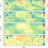 |
Fig. 6 Reddening maps available for the NB region from different authors. A: this work. B: Sanders et al. (2022). C: Zelakiewicz et al. (2025). D: Surot et al. (2020). The map in panel D uses J instead of H. In all panels, a dimmed dashed white rectangle shows the location of the Brick, as shown in Fig. 7. |
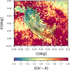 |
Fig. 7 Zoom-in of Fig. 6 of the Brick region. The color bar is optimized to highlight the gradient in E(H-K) over the Brick. The northern part of the Brick is less extincted than the southern part. The contours show the column density maps from Marsh et al. (2017) in units of 1020 cm−2. |
4 Stellar mass estimation through RC star counts
One way to estimate the stellar mass is through RC star counts, as described in Valenti et al. (2016). Computing the mass on each NBF led us to improve the mass profile shown in their Fig. 4 by adding five points instead of one point in their most central bin, where all NBFs are located (see the inset of Fig. 10). To achieve this goal, we performed the following steps: first, we corrected the observed star counts for completeness. Then, we dereddened the K LF and subtracted the contribution by the RGB stars. Finally, we converted the number of RC stars into mass using a fully empirical approach.
4.1 Artificial star tests
We estimated the probability of each star being detected given its position in the sky and locus in the CMD by performing artificial star tests (ASTs). This classical technique is widely used in the literature (see e.g., Aparicio & Gallart 1995; Gallart et al. 1996; Harris & Speagle 2024, Sect. 2 for a review). Because the RC spans a significant range in magnitude and in color due to extinction, stars were very generously injected within a CMD box encompassing the whole RC region (Fig. 8). A flat distribution was used for K magnitude and H-K color.
The stars were injected in a hexagonal grid designed to avoid artificial crowding (see Piotto & Zoccali 1999; Zoccali et al. 1999, 2003). We used a separation of 40 pixels between artificial stars (∼2 PSF fitting radius), which allowed us to inject ∼3000 stars simultaneously per chip per iteration. We repeated the process 31 times to obtain ∼2 000 000 artificial stars in all the NBFs.
To estimate the completeness, we used the recovery fraction, which is the ratio of recovered and injected stars at a given locus in the CMD (Aparicio & Gallart 1995). To assess the different crowding levels in the images, we created Voronoi bins where the crowding was approximately the same. Within each bin, we modeled the completeness as a logistic function and fitted it to the observed recovery fraction in color and magnitude at the same time. With this model, we assigned detection probabilities to each real star. Stars outside the box were extrapolated from the model.
In Fig. 8m we show the CMD of all NBF fields colored by detection probability. As expected, the brighter less extincted stars have higher detection probabilities than the fainter more extincted ones. We also verified that RC stars are in a high-completeness region. The bulk of RC stars is located in the 90% completeness region, whereas the most extincted RC stars have a completeness between 70% and 80%. We also verified that the 50% probability detection level was at K = 18.0 ± 0.3, H-K = 2.0 ± 0.3, which is fainter by three magnitudes than the peak of the observed RC. This is an improvement over previous completeness estimates in this region. Valenti et al. (2016) showed in their Fig. 1 a completeness below 50% for this region at the dereddened magnitude of the RC, which they also obtained with AST. The 50% completeness threshold is important because it is one way to define the limiting magnitude (e.g., Harris 1990). Moreover, Nogueras-Lara et al. (2020) estimated a completeness of 80% at magnitude KS ∼16, which is somewhat smaller than our completeness estimates at the same magnitude. However, they did not use AST to estimate completeness, which, along with the different observation strategy of GNC, might explain this difference.
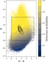 |
Fig. 8 Same Hess diagram as Fig. 3, but colored by detection probability. The injection region is shown as the dashed black rectangle, between 12 ≤ K ≤ 18 and 0 ≤ H-K ≤ 4.5. The black contours show the quintile levels of the RC density. |
4.2 Stellar density profile
In this section, we derive the stellar density profile based on the dereddened LF of RC stars. We adopted an intrinsic color for the RC of (H-K)0 = 0.114. This is the color of the chosen anchor point (see Sect. 3.2), hence it is not exactly the RC intrinsic color, as our reference fields do have some reddening. Nonetheless, this value is only slightly higher than the intrinsic color adopted by Plevne et al. (e.g. 2020); Nogueras-Lara et al. (e.g. 2020, 2021b), as expected, given that the chosen reference fields are all low-reddening windows.
In each NBF field, we corrected the observed star counts by weighing the dereddened LF by the inverse of the detection probability, obtained from the completeness analysis. To obtain the number of RC stars, we discounted the contribution of RGB stars in the LF, as shown in the left panel of Fig. 9. We fitted the RGB with a cubic spline in the areas next to the RC in the LF, depicted as the gray areas of Fig. 9. Next, we subtracted the spline from the LF and obtained the histogram shown in the right panel of Fig. 9. Then, we used the BayesianGaussianMixture algorithm from scikit-learn to find the best composition of Gaussian functions that describe the LF with the RGB substracted. In all the NBFs, we found that the data are well described with three distributions, which we interpret as the early-AGB phase, the RC stars, and the RGB-bump. We also note that the fit shows a peak in the residuals at K0 ~13. This peak might arise because the shape of the RC in the LF is not perfectly described by a Gaussian. Nevertheless, the residuals are symmetric around zero, without a systematic trend, which indicates that the fit is unbiased.
Fig. 10 compares star count results with those of Valenti et al. (2016, their Fig. 4). To do this, we normalized the counts to the same unit of area. Our area is much smaller than the VVV area: all of our fields lie within their innermost field, as shown by the inset of Fig. 10. The purpose of this section is to provide a density and a mass profile with higher spatial resolution in the NB of the MW, where the spatial gradient is very steep, and an average of 1° × 1° field cannot appropriately describe the real profile. The innermost point of the profile of Valenti et al. (2016) is the mean of the high density of the NB with a much lower density of a larger area surrounding it. It clearly is lower by a factor of 10 than the real density of the nuclear region, which we provided with our finer spatial sampling in the inner region.
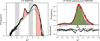 |
Fig. 9 Star counts of field NBF054. Left: K0LF of field NBF054. The black line shows the star counts corrected by completeness. For comparison, the gray line represents the uncorrected LF. The spline modeling the RGB is shown as dashed green lines. The fitting regions for the spline are shown as the vertical gray area. The LF with subtracted RGB LF is represented with the red area. Right: K0 LF with RGB subtracted is represented by the solid red histogram. Three Gaussians were fitted to the data: the left and right gray ones represent the early-AGB and RGB-bump, respectively; and the central green one represents the RC star counts. The solid black line represents the sum of the three Gaussians. The residuals to the fit are shown in the bottom part of the panel. |
4.3 Estimation of the stellar mass
To convert RC star counts into stellar mass, we relied on the measurements by Valenti et al. (2016) of the mass of the MW bulge. Their method employs a three-step scaling approach that begins with the empirical IMF derived from HST/NICMOS observations in a small bulge field (Zoccali et al. 2000; Calamida et al. 2015). Then, it is scaled up to a medium-sized NTT/SOFI, as discussed in Zoccali et al. (2003, their Sect. 5) using the area ratio of the two observations, and it is finally extrapolated to the entire VVV survey area by comparing RGB and RC star counts between the SOFI field and the full VVV footprint (Valenti et al. 2016).
Valenti et al. (2016) found a total mass of the MW bulge of 2.0 × 10¹⁰ M⊙. Their bin was centered in (l, b) = (0°, 0°) and had a mass of 3.2 × 10⁸ M⊙ (their Fig. 5) with 315 274 RC stars (private communication and their Fig. 4), meaning that each RC star traced 1015 M⊙ of stellar mass. On the other hand, in all the NBFs, we found a total of 182 729 RC stars, which means that we trace a total stellar mass of 1.85 ± 0.3 × 10⁸ M⊙ within the region we studied. Since our data only cover the innermost part of the NB, we scaled the observed mass up by considering the ratio of the observed area of NBFs and the NSD extent as reported by Sormani et al. (2022). We considered a box defined by their radial scale length and scale height as the extent of the NSD model, with values of 88.6 pc and 28.4 pc, respectively. This gives an area ratio of ~6.6 of the full NSD model and the NBF footprint. We assumed a uniform distribution of stellar mass across these areas, which is a simplification of the density gradient of this structure. With this scale factor, our scaled mass of the NB is 12.2 ± 2.6 × 10⁸ M⊙. The uncertainties of the stellar mass and a comparison of our measurement with model predictions and literature estimates are presented in Sect. 5.5.
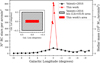 |
Fig. 10 Stellar density profile, in the number of stars per arcmin2 as function of the Galactic longitude. The black triangles show the density profile computed by Valenti et al. (2016) in their Fig. 4 at b = 0°. The red triangles represent the five fields we studied in this work. The inset shows a comparison between the spatial extent of both works. The hatched black square represents the innermost bin of Valenti et al. (2016), whereas the filled red rectangle is the area covered in this study. The right axis shows the star counts converted into stellar mass per arcmin2 . The difference in the spatial coverage explains the marked difference in RC star density. |
5 Discussion
5.1 The distance-extinction degeneracy in the NBFs
There is a difference between the extinction ratios computed with our kinematic method and those derived from a direct linear fit to the RC in the NBFs. The linear fit produces a slope of 1.456, which differs from our total-to-selective extinction ratio of 1.256 ± 0.076 by more than 2σ. This discrepancy comes from a distance-extinction degeneracy that affects the observed RC slope in the NBFs. As shown in panels C and E of Fig. 5, less strongly extincted stars have systematically different proper motions than more strongly extincted stars, indicating that they are not at the same distance. Stars with lower extinction are located preferentially in the foreground, whereas stars with high extinction are located preferentially in the background. Hence, the observed spread in K magnitude along the observed RC sequence arises from a superposition of increasing extinction and distance modulus, and the RC slope therefore overestimates the total-to-selective extinction ratio.
We verified this quantitatively. For AK/E(H – K) = 1.456 and an intrinsic color of (H-K)0 = 0.1, the dereddened RC locus lies at (H – K, K) = (0.1,12.61). Then, assuming an absolute magnitude of MK = −1.60, we obtain a distance of ~6.9 kpc to the bulk of the RC stars, which is significantly shorter than the well-established distance to the GC. By contrast, forcing the fit to pass through the anchor RC position breaks this degeneracy and produces a physically consistent slope of AK/E(H-K) = 1.265. Since the distance to the GC is well established (e.g., GRAVITY Collaboration 2022), we relied on the anchor RC as a robust constraint on the fit.
These results might alternatively be interpreted to show that the bulk of RC stars is located in front of the GC, but this lacks a physical justification. There is no reason to expect a concentration of RC stars at ~6.9 kpc along this LOS. We therefore conclude that our method breaks the distance-extinction degeneracy and recovers the intrinsic extinction law.
5.2 Comparison with previous extinction ratios
Our ratios agree well with works that used RC stars to trace the extinction law in the GC region. Schödel et al. (2010) measured the total extinction in RC stars by adopting an absolute magnitude of the RC stars MK = −1.54 (Groenewegen 2008), a mean distance to the GC of R0 = 8.03 kpc, and an intrinsic color of H-K = 0.07. With this, they estimated an absolute extinction ratio of AH/AK = 1.76. One key point is that Schödel et al. (2010) only used stars within a FoV of 40″ × 40″ around Sgr A*, whereas our spatial coverage is ~630 times larger than theirs.
Despite the difference in spatial coverage, the results are consistent, meaning that the extinction properties near the GC are compatible with the extended ones of the NB.
With a wider spatial coverage, Nogueras-Lara et al. (2020) computed extinction ratios using the RC method in the CMD of different regions of the GNC project in J, H, and Ks filters. For their central region, which overlaps most with our NBFs fields, they found an extinction index of αHK = 2.20, which we converted into the total-to-selective extinction ratio using their Equation (1), obtaining AK/EH-K = 1.22. They also reported an absolute extinction ratio of AH/AK = 1.84. Their RC slope differs from the slope we measured in Sect. 3.1. To double-check our results, we measured the slope using the same method as Nogueras-Lara et al. (2020), by binning by color and applying a Gaussian mixture model to each bin. We found a RC slope of 1.44, which is consistent with the measurement of the unsharpmasking method. Although the methods are very different, the extinction ratios are similar.
Interestingly, our kinematic derivation of the extinction ratios is consistent with other methods and tracers. Sanders et al. (2022) used a multiwavelength approach using the RC method plus the Rayleigh-Jeans color-excess method in the inner 3° × 3° of the Galaxy. Their measurements of the total-to-selective extinction ratio and absolute extinction ratio are very similar to our independent measurement, with values of AK/EH-K = 1.293 and AH/AK = 1.77, respectively. Our results also agree with methods that used variable stars as tracers. Minniti et al. (2020) used classical Cepheids to trace the disk structure on the far side of the MW bulge, and they also derived extinction ratios by measuring the color-excess ratios and knowing the intrinsic colors of these variable stars. They obtained AK/EH-K = 1.30 and AH/AK = 1.76. Albarracín et al. (2025) performed a similar work with Mira variables and found AK/EH-K = 1.32. All of these results indicate a convergence of the extinction ratios toward the NB of the MW. Finally, Bravo Ferres et al. (2025) found AK/EH-K = 1.69 ± 0.04 using the James Webb Space Telescope (JWST) in the Sagittarius C region, similar to our measurement.
Our results differ from the classical extinction ratios assumed for the rest of the Galaxy. The total-to-selective extinction ratios from Nishiyama et al. (2006, 2009) are AK/EH-K = 1.44 and AK/EH-K = 1.61 respectively. They were computed using the RC method, but in the outer parts of the MW bulge. Moreover, Alonso-García et al. (2017) used the same method in the VVV survey filters and found AK/EH-K = 1.104 for the bulge. As they stated, this value varies depending on the selected LOS.
We present a summary of the works with which we compared our results in Table 1. The extinction ratios are stable for different methods and tracers, suggesting they are not strongly sensitive to the specific technique employed. Therefore, we consider the extinction ratios we derived robust for this region of the MW.
Absolute and total-to-selective extinction ratios from previous works.
5.3 Assumptions of the RC method
The RC method has some underlying assumptions that we need to address for the NB. First, it assumes that all stars are at the same distance, or at least that the spread along the LOS is negligible compared to the distance to the object of study. This assumption is true for studies of satellite galaxies (i.e., the LMC and SMC), but not for the NB. Here, the expected LOS spread is about 400 pc, which represents a variation of ~0.1 magnitudes at 8.2 kpc. If the spread along the LOS is not carefully addressed, it might be misinterpreted as population effects.
This led us to a second assumption: the intrinsic brightness of RC stars varies little with age and metallicity distribution. This is true for stars older than 1 Gyr (see Girardi 2016), and it underpins the RC method and our kinematic selection of RC stars for measuring the extinction law. In the NB, however, we expect a spread in both metallicity (Fritz et al. 2021, their Fig. 10) and age. The latter is expected based on the inside-out formation that is observed in extragalactic nuclear regions (Bittner et al. 2020), and it was detected in the MW NSD by Nogueras-Lara et al. (2023). Nogueras-Lara et al. (2020) concluded that about 90% of the stellar mass of the NSD was formed over 8 Gyr ago, 5% was formed about 1 Gyr ago, and the remaining 5% is less than 0.1 Gyr old. To reach this conclusion, they decomposed the GNC dereddened completeness-corrected KS LF as a linear combination of theoretical LFs for different stellar populations. Although simple, this method can be subject to up to 20% error when systematic effects are not considered (Girardi 2016).
While the RC method is robust to moderate variations in these parameters, we caution that the distribution of star ages in the NB remains uncertain. This could introduce errors in our measurements, particularly in the interpretation that the peak of the LF around (H-K)KC0 corresponds to stars at the distance of the GC (see Sect. 3.3).
5.4 Interpretation of RC distributions in the NB
The RC distribution in the NB shows structures that are not completely understood, and their interpretation demands caution. For example, Zoccali et al. (2021) questioned the distance used for the Brick. They found that the RC on top of the Brick is significantly brighter than an RC in a control field. This vertical offset was interpreted as a distance difference, placing the Brick at 7.2 kpc from the Sun. Later, Nogueras-Lara et al. (2021b) computed the distance using two methods: 1) a linear fit to the observed RC to recover the mean reddening-free KS magnitude, and 2) by fitting the dereddened RC LF to obtain the mean distance to the Brick. With the former method, they obtained a distance of 7.6 kpc, whereas using the latter, they derived 8.4 kpc. Additionally, Lipman et al. (2025) computed the probability of a group of dense clouds located in the direction of the NB to be on the near or far side of the NB. They used the 8 μm and 70 μm dust extinction method on a GLIMPSE residual map from the Spitzer telescope (Benjamin et al. 2003; Churchwell et al. 2009), and the Hi-GAL (Molinari et al. 2010, 2016) 70 μm emission and the computed column densities. They obtained that the Brick most likely lies on the near side of the NB.
Our map shows that the mean reddening above the Brick is lower than in its surroundings, which supports the hypothesis that the Brick lies in front of the NB. However, there is no gradient in gas density or continuum emission along the major axis of the Brick, which cannot explain the gradient observed in IR extinction, as observed in Fig. 7. Although it is a reasonable assumption that the Brick lies in the NB, the differences in the results for different methods indicate an underlying problem in interpreting the RC distribution and a complex 3D structure of the Brick (Henshaw et al. 2019).
Furthermore, the LF distribution in Fig. 9 shows three components, two of which are clearly the AGB bump and RC. However, the interpretation of the third fainter component is not clear. We interpret this faint component as a metal-rich RGB-bump, since for the observed metallicities in the NB it should fall below the RC (e.g., Valenti et al. 2004). However, Nogueras-Lara et al. (2020) interpreted the same feature in their data as a secondary RC, which they associated with a younger population in the NB. The ambiguity between these two interpretations highlights the complexity of the stellar populations in the NB, and it underscores the need for a broader parameter space to separate its different components.
5.5 Stellar mass comparison with models and literature
To compare our results with model predictions over the same spatial footprint, we used the software AGAMA (Vasiliev 2019) to evaluate the stellar mass density of the Sormani et al. (2022) and Hunter et al. (2024) models. We drew 106 random points uniformly distributed within a volume defined by the NBF longitude and latitude and in a distance range of 7–9 kpc. The distance range was chosen to enclose the NSD, which dominates the stellar mass along this LOS, and to include any foreground and background contamination. We computed the enclosed mass as the product of the mean model density and the sampled volume. For Sormani et al. (2022), we found 0.73 × 10⁸ M⊙, whereas for Hunter et al. (2024), we found 1.63 × 10⁸ M⊙. Our observed mass of 1.85 × 10⁸ M⊙ is consistent with predictions from dynamical models for this region of the MW.
The uncertainty in the stellar mass estimate has two main contributions. The first contribution comes from the mass traced by each RC star, for which we adopted the 15% conservative uncertainty reported by Valenti et al. (2016), which accounts for the IMF slope, disk contamination, and stellar population gradients. This yields an observed stellar mass of 1.85 ± 0.30 × 10⁸ M⊙. This error dominates other sources of uncertainty, such as the Poisson error when counting RC stars, or the uncertainty in the RGB subtraction from the K0 LF.
The second contribution of uncertainty comes from the area scaling, which assumes a uniform surface density across the NSD model. Since the NBF samples the densest part of the NSD model, this assumption likely overestimates the total mass and introduces an additional systematic uncertainty, which we conservatively estimated to be at the same level of the first: 15%. Applying both contributions to the scaled mass and combining them in quadrature, we obtained a total uncertainty of ∆M = 2.6 × 10⁸ M⊙ and a final scaled mass of 12.2 ± 2.6 × 10⁸ M⊙ for the NB region.
This value agrees with the reported mass estimates in the NB, as shown in Table 2. Sormani et al. (2020a) found a dynamical mass of 6.9 ± 2 × 10⁸ M⊙ by applying a Jeans modeling to the NSD region. Li et al. (2022) used this value in hydrodynamical simulations with updated potentials for the region (see their Table 1) and verified that an NSD with this stellar mass can reproduce a gas disk similar to the observed CMZ. Later, Sormani et al. (2022) updated their result to 10.5 ± 1 × 10⁸ M⊙ with a self-consistent dynamical model. Even earlier than these measurements, Launhardt et al. (2002) estimated a mass of 14.2 ± 6 × 10⁸ M⊙ in the NB region by assuming a fixed mass-to-light ratio. Neither this former estimate nor ours relied on dynamical models for the mass estimation in the NB. Our empirical measurement is consistent with these results within the reported errors.
Mass estimates in the nuclear bulge region compared with the literature.
5.6 Future prospects
As shown above, it is essential to study the stellar content of the NB to obtain a comprehensive view of the structure and processes that occur here. In this region, a joint analysis of the stellar content and gas-phase structures is not only powerful, but also imperative. Moreover, data from new NIR facilities are essential for future studies: the JWST can reach down to magnitude ~24 in the F210M filter (similar to Ks) with NIRCAM. This means that we could detect MS stars and measure the NB IMF. This might also allow us to obtain better estimates of the SFH of the NB because main-sequence turn-off stars are expected to be at a magnitude of ~ 19-20.
6 Summary
We studied the NB stellar content to obtain new insights into its structure and to place observational constraints. We used RC stars to trace the extinction and to empirically estimate the stellar mass we can observe in this region.
We developed a novel method to estimate the extinction law toward the NB using the kinematics of the RC stars. This method assumes that the RC density peak is located at the distance of the GC and that stars on the near side of the GC have different kinematics from those on the far side. We found a total-to-selective extinction ratio of AK/EH-K = 1.259 ± 0.074 and an absolute extinction ratio of AK/AH = 1.794 ± 0.046. These values are in the same range as previous works in the nuclear regions of the MW, but they differ from those derived using stars outside these regions. This suggests that the extinction law is dependent on the LOS. With these extinction ratios, we built a reddening map with a high spatial resolution, which is the most detailed map for this region so far. Its most noticeable characteristics are the gradient on top of the Brick, which does not correlate with gas density maps, and the filamentary structures toward negative longitudes. We discussed the potential sources of errors and caveats associated with tracing structures using RC stars.
Finally, new-generation instrumentation and telescopes, such as MICADO (Davies et al. 2021), MOSAIC Hammer et al. (2021), and HARMONI (Thatte et al. 2021) at the Extremely Large Telescope (ELT), will revolutionize the study of the NB, and it presents an interesting scientific case for future space projects, such as JASMINE (Kawata et al. 2024) and GaiaNIR (Hobbs et al. 2016).
Data availability
The full version of Table C.1 is available at the CDS via https://cdsarc.cds.unistra.fr/viz-bin/cat/J/A+A/711/A232
Acknowledgements
We acknowledge the referee for their comments, which polished this article to its current version. A.V.N. thanks D. Riquelme, C. Ordenes-Huanca, B. Acosta-Tripailao, and C. Quezada, for their insightful discussions and helpful advice about this work. A.V.N. also acknowledges support from the National Agency for Research and Development (ANID) Scholarship Program Doctorado Nacional 2020–21201226. Also acknowledges partial funding of ANID BASAL Center for Astrophysics and Associated Technologies (CATA) FB210003, by the ANID Millennium Science Initiative, ICN12_009 and AIM23-0001, awarded to the Millennium Institute of Astrophysics (MAS), and ESO SSDF Project 21/24. M.Z. acknowledges support from FONDECYT Regular grant No. 1230731. E.V. acknowledges the Excellence Cluster ORIGINS Funded by the Deutsche Forschungsgemeinschaft (DFG, German Research Foundation) under Germany’s Excellence Strategy – EXC-2094-390783311. CG acknowledges support from the Agencia Estatal de Investigación del Ministerio de Ciencia e Innovación (AEI-MCINN) under grants “At the forefront of Galactic Archaeology: evolution of the luminous and dark matter components of the Milky Way and Local Group dwarf galaxies in the Gaia era” with reference PID2023-150319NB-C21/10.13039/501100011033. F.G. gratefully acknowledges support from the French National Research Agency (ANR) funded project “MWDisc” (ANR-20-CE31-0004) and “Pristine” (ANR-18-CE31-0017). F.G. also acknowledges support from the Research fellow Gemini-ANID 2025 – 32RF250005 project, and the international Gemini Observatory, a program of NSF NOIRLab, which is managed by the Association of Universities for Research in Astronomy (AURA) under a cooperative agreement with the U.S. National Science Foundation, on behalf of the Gemini partnership of Argentina, Brazil, Canada, Chile, the Republic of Korea, and the United States of America. This work made use of a number of tools and python packages: Astropy:6 a community-developed core Python package and an ecosystem of tools and resources for astronomy (Astropy Collaboration 2013, 2018, 2022), Numpy (Harris et al. 2020), Scipy (Virtanen et al. 2020), the Scikit-learn library (Pedregosa et al. 2011), Pandas (pandas development team 2020), astroML (Van-derplas et al. 2012), Aladin (Bonnarel et al. 2000), and Topcat (Taylor 2017).
References
- Alard, C. 2001, A&A, 379, L44 [NASA ADS] [CrossRef] [EDP Sciences] [Google Scholar]
- Albarracín, R., Zoccali, M., Olivares Carvajal, J., et al. 2025, A&A, 693, A28 [NASA ADS] [CrossRef] [EDP Sciences] [Google Scholar]
- Alonso-García, J., Dékány, I., Catelan, M., et al. 2015, AJ, 149, 99 [CrossRef] [Google Scholar]
- Alonso-García, J., Minniti, D., Catelan, M., et al. 2017, ApJ, 849, L13 [Google Scholar]
- Aparicio, A., & Gallart, C. 1995, AJ, 110, 2105 [Google Scholar]
- Arsenault, R., Madec, P. Y., Hubin, N., et al. 2008, SPIE Conf. Ser., 7015, 701524 [NASA ADS] [Google Scholar]
- Astropy Collaboration (Robitaille, T. P., et al.) 2013, A&A, 558, A33 [NASA ADS] [CrossRef] [EDP Sciences] [Google Scholar]
- Astropy Collaboration (Price-Whelan, A. M., et al.) 2018, AJ, 156, 123 [Google Scholar]
- Astropy Collaboration (Price-Whelan, A. M., et al.) 2022, ApJ, 935, 167 [NASA ADS] [CrossRef] [Google Scholar]
- Baba, J., & Kawata, D. 2020, MNRAS, 492, 4500 [NASA ADS] [CrossRef] [Google Scholar]
- Benjamin, R. A., Churchwell, E., Babler, B. L., et al. 2003, PASP, 115, 953 [Google Scholar]
- Bittner, A., Sánchez-Blázquez, P., Gadotti, D. A., et al. 2020, A&A, 643, A65 [NASA ADS] [CrossRef] [EDP Sciences] [Google Scholar]
- Bonnarel, F., Fernique, P., Bienaymé, O., et al. 2000, A&AS, 143, 33 [Google Scholar]
- Bravo Ferres, L., Nogueras-Lara, F., Schödel, R., et al. 2025, A&A, 704, A130 [NASA ADS] [CrossRef] [EDP Sciences] [Google Scholar]
- Calamida, A., Sahu, K. C., Casertano, S., et al. 2015, ApJ, 810, 8 [NASA ADS] [CrossRef] [Google Scholar]
- Cardelli, J. A., Clayton, G. C., & Mathis, J. S. 1989, ApJ, 345, 245 [Google Scholar]
- Casali, M., Pirard, J.-F., Kissler-Patig, M., et al. 2006, SPIE Conf. Ser., 6269, 62690W [Google Scholar]
- Churchwell, E., Babler, B. L., Meade, M. R., et al. 2009, PASP, 121, 213 [Google Scholar]
- Davies, R., Hörmann, V., Rabien, S., et al. 2021, The Messenger, 182, 17 [NASA ADS] [Google Scholar]
- De Marchi, G., Panagia, N., Sabbi, E., et al. 2016, MNRAS, 455, 4373 [CrossRef] [Google Scholar]
- de Sá-Freitas, C., Fragkoudi, F., Gadotti, D. A., et al. 2023, A&A, 671, A8 [NASA ADS] [CrossRef] [EDP Sciences] [Google Scholar]
- de Sá-Freitas, C., Gadotti, D. A., Fragkoudi, F., et al. 2025, A&A, 698, A5 [NASA ADS] [CrossRef] [EDP Sciences] [Google Scholar]
- Fragkoudi, F., Athanassoula, E., & Bosma, A. 2016, MNRAS, 462, L41 [NASA ADS] [CrossRef] [Google Scholar]
- Fritz, T. K., Patrick, L. R., Feldmeier-Krause, A., et al. 2021, A&A, 649, A83 [NASA ADS] [CrossRef] [EDP Sciences] [Google Scholar]
- Gadotti, D. A., Sánchez-Blázquez, P., Falcón-Barroso, J., et al. 2019, MNRAS, 482, 506 [Google Scholar]
- Gallart, C., Aparicio, A., & Vilchez, J. M. 1996, AJ, 112, 1928 [NASA ADS] [CrossRef] [Google Scholar]
- Girardi, L. 2016, ARA&A, 54, 95 [Google Scholar]
- Gonzalez, O. A., Minniti, D., Valenti, E., et al. 2018, MNRAS, 481, L130 [Google Scholar]
- GRAVITY Collaboration. 2019, A&A, 625, L10 [NASA ADS] [CrossRef] [EDP Sciences] [Google Scholar]
- GRAVITY Collaboration. 2022, A&A, 657, L12 [NASA ADS] [CrossRef] [Google Scholar]
- Groenewegen, M. A. T. 2008, A&A, 488, 935 [CrossRef] [EDP Sciences] [Google Scholar]
- Hammer, F., Morris, S., Cuby, J.-G., et al. 2021, The Messenger, 182, 33 [NASA ADS] [Google Scholar]
- Harris, W. E. 1990, PASP, 102, 949 [Google Scholar]
- Harris, W. E., & Speagle, J. S. 2024, AJ, 168, 38 [Google Scholar]
- Harris, C. R., Millman, K. J., van der Walt, S. J., et al. 2020, Nature, 585, 357 [NASA ADS] [CrossRef] [Google Scholar]
- Henshaw, J. D., Ginsburg, A., Haworth, T. J., et al. 2019, MNRAS, 485, 2457 [Google Scholar]
- Henshaw, J. D., Barnes, A. T., Battersby, C., et al. 2023, in Astronomical Society of the Pacific Conference Series, 534, Protostars and Planets VII, eds. S. Inutsuka, Y. Aikawa, T. Muto, K. Tomida, & M. Tamura, 83 [Google Scholar]
- Hobbs, D., Høg, E., Mora, A., et al. 2016, arXiv e-prints [arXiv:1609.07325] [Google Scholar]
- Hosek, Jr., M. W., Lu, J. R., Anderson, J., et al. 2018, ApJ, 855, 13 [Google Scholar]
- Hosek, M. W., Do, T., Lu, J. R., et al. 2022, ApJ, 939, 68 [NASA ADS] [CrossRef] [Google Scholar]
- Hunter, G. H., Sormani, M. C., Beckmann, J. P., et al. 2024, A&A, 692, A216 [NASA ADS] [CrossRef] [EDP Sciences] [Google Scholar]
- Indebetouw, R., Mathis, J. S., Babler, B. L., et al. 2005, ApJ, 619, 931 [NASA ADS] [CrossRef] [Google Scholar]
- Kawata, D., Kawahara, H., Gouda, N., et al. 2024, PASJ, 76, 386 [Google Scholar]
- Kennicutt, Jr., R. C. 1998, ApJ, 498, 541 [Google Scholar]
- Kissler-Patig, M., Pirard, J. F., Casali, M., et al. 2008, A&A, 491, 941 [NASA ADS] [CrossRef] [EDP Sciences] [Google Scholar]
- Kruijssen, J. M. D., & Longmore, S. N. 2013, MNRAS, 435, 2598 [Google Scholar]
- Launhardt, R., Zylka, R., & Mezger, P. G. 2002, A&A, 384, 112 [NASA ADS] [CrossRef] [EDP Sciences] [Google Scholar]
- Li, Z., Shen, J., Gerhard, O., & Clarke, J. P. 2022, ApJ, 925, 71 [CrossRef] [Google Scholar]
- Lipman, D., Battersby, C., Walker, D. L., et al. 2025, ApJ, 984, 159 [Google Scholar]
- Longmore, S. N., Bally, J., Testi, L., et al. 2013, MNRAS, 429, 987 [NASA ADS] [CrossRef] [Google Scholar]
- Marsh, K. A., Whitworth, A. P., Lomax, O., et al. 2017, MNRAS, 471, 2730 [Google Scholar]
- Martínez-Arranz, Á., Schödel, R., Nogueras-Lara, F., & Shahzamanian, B. 2022, A&A, 660, L3 [NASA ADS] [CrossRef] [EDP Sciences] [Google Scholar]
- Mezger, P. G., Duschl, W. J., & Zylka, R. 1996, A&A Rev., 7, 289 [Google Scholar]
- Minniti, D., Lucas, P. W., Emerson, J. P., et al. 2010, New Astron., 15, 433 [Google Scholar]
- Minniti, J. H., Sbordone, L., Rojas-Arriagada, A., et al. 2020, A&A, 640, A92 [EDP Sciences] [Google Scholar]
- Molinari, S., Swinyard, B., Bally, J., et al. 2010, A&A, 518, L100 [NASA ADS] [CrossRef] [EDP Sciences] [Google Scholar]
- Molinari, S., Schisano, E., Elia, D., et al. 2016, A&A, 591, A149 [NASA ADS] [CrossRef] [EDP Sciences] [Google Scholar]
- Nishiyama, S., Nagata, T., Kusakabe, N., et al. 2006, ApJ, 638, 839 [Google Scholar]
- Nishiyama, S., Tamura, M., Hatano, H., et al. 2009, ApJ, 696, 1407 [NASA ADS] [CrossRef] [Google Scholar]
- Nogueras-Lara, F., Schödel, R., Gallego-Calvente, A. T., et al. 2019, A&A, 631, A20 [NASA ADS] [CrossRef] [EDP Sciences] [Google Scholar]
- Nogueras-Lara , F., Schödel, R., Gallego-Calvente, A. T., et al. 2020, Nat. Astron., 4, 377 [Google Scholar]
- Nogueras-Lara, F., Schödel, R., Neumayer, N., et al. 2020, A&A, 641, A141 [EDP Sciences] [Google Scholar]
- Nogueras-Lara, F., Schödel, R., & Neumayer, N. 2021a, A&A, 653, A133 [NASA ADS] [CrossRef] [EDP Sciences] [Google Scholar]
- Nogueras-Lara, F., Schödel, R., Neumayer, N., & Schultheis, M. 2021b, A&A, 647, L6 [NASA ADS] [CrossRef] [EDP Sciences] [Google Scholar]
- Nogueras-Lara, F., Schultheis, M., Najarro, F., et al. 2023, A&A, 671, L10 [NASA ADS] [CrossRef] [EDP Sciences] [Google Scholar]
- pandas development team, T. 2020, pandas-dev/pandas: Pandas [Google Scholar]
- Paufique, J., Bruton, A., Glindemann, A., et al. 2010, SPIE Conf. Ser., 7736, 77361P [Google Scholar]
- Pedregosa, F., Varoquaux, G., Gramfort, A., et al. 2011, J. Mach. Learn. Res., 12, 2825 [Google Scholar]
- Piotto, G., & Zoccali, M. 1999, A&A, 345, 485 [NASA ADS] [Google Scholar]
- Pirard, J.-F., Kissler-Patig, M., Moorwood, A., et al. 2004, SPIE Conf. Ser., 5492, 1763 [Google Scholar]
- Plevne, O., Önal Tas¸, Ö., Bilir, S., & Seabroke, G. M. 2020, ApJ, 893, 108 [NASA ADS] [CrossRef] [Google Scholar]
- Portail, M., Wegg, C., Gerhard, O., & Martinez-Valpuesta, I. 2015, MNRAS, 448, 713 [NASA ADS] [CrossRef] [Google Scholar]
- Rathborne, J. M., Longmore, S. N., Jackson, J. M., et al. 2014, ApJ, 786, 140 [Google Scholar]
- Reid, M. J., & Brunthaler, A. 2020, ApJ, 892, 39 [Google Scholar]
- Renzini, A., Gennaro, M., Zoccali, M., et al. 2018, ApJ, 863, 16 [NASA ADS] [CrossRef] [Google Scholar]
- Rodriguez-Fernandez, N. J., & Combes, F. 2008, A&A, 489, 115 [CrossRef] [EDP Sciences] [Google Scholar]
- Saito, R. K., Hempel, M., Alonso-García, J., et al. 2024, A&A, 689, A148 [NASA ADS] [CrossRef] [EDP Sciences] [Google Scholar]
- Sanders, J. L., Smith, L., González-Fernández, C., Lucas, P., & Minniti, D. 2022, MNRAS, 514, 2407 [CrossRef] [Google Scholar]
- Schlafly, E. F., Meisner, A. M., & Green, G. M. 2019, ApJS, 240, 30 [Google Scholar]
- Schmidt, M. 1959, ApJ, 129, 243 [NASA ADS] [CrossRef] [Google Scholar]
- Schödel, R., Najarro, F., Muzic, K., & Eckart, A. 2010, A&A, 511, A18 [Google Scholar]
- Schödel, R., Yelda, S., Ghez, A., et al. 2013, MNRAS, 429, 1367 [Google Scholar]
- Schödel, R., Nogueras-Lara, F., Hosek, M., et al. 2023, A&A, 672, L8 [NASA ADS] [CrossRef] [EDP Sciences] [Google Scholar]
- Schönrich, R., Aumer, M., & Sale, S. E. 2015, ApJ, 812, L21 [Google Scholar]
- Schultheis, M., Fritz, T. K., Nandakumar, G., et al. 2021, A&A, 650, A191 [NASA ADS] [CrossRef] [EDP Sciences] [Google Scholar]
- Schultheis, M., Sormani, M. C., & Gadotti, D. A. 2025, A&A Rev., 33, 7 [Google Scholar]
- Siebenmorgen, R., Carraro, G., Valenti, E., et al. 2011, The Messenger, 144, 9 [NASA ADS] [Google Scholar]
- Simion, I. T., Belokurov, V., Irwin, M., et al. 2017, MNRAS, 471, 4323 [NASA ADS] [CrossRef] [Google Scholar]
- Skrutskie, M. F., Cutri, R. M., Stiening, R., et al. 2006, AJ, 131, 1163 [NASA ADS] [CrossRef] [Google Scholar]
- Smith, L. C., Lucas, P. W., Koposov, S. E., et al. 2025, MNRAS, 536, 3707 [NASA ADS] [CrossRef] [Google Scholar]
- Sormani, M. C., Magorrian, J., Nogueras-Lara, F., et al. 2020a, MNRAS, 499, 7 [Google Scholar]
- Sormani, M. C., Tress, R. G., Glover, S. C. O., et al. 2020b, MNRAS, 497, 5024 [Google Scholar]
- Sormani, M. C., Sanders, J. L., Fritz, T. K., et al. 2022, MNRAS, 512, 1857 [CrossRef] [Google Scholar]
- Stanek, K. Z., Mateo, M., Udalski, A., et al. 1994, ApJ, 429, L73 [NASA ADS] [CrossRef] [Google Scholar]
- Stanek, K. Z., Udalski, A., SzymaŃski, M., et al. 1997, ApJ, 477, 163 [NASA ADS] [CrossRef] [Google Scholar]
- Stetson, P. B. 1987, PASP, 99, 191 [Google Scholar]
- Stetson, P. B. 1994, PASP, 106, 250 [Google Scholar]
- Stolte, A., Hußmann, B., Olczak, C., et al. 2015, A&A, 578, A4 [NASA ADS] [CrossRef] [EDP Sciences] [Google Scholar]
- Surot, F., Valenti, E., Gonzalez, O. A., et al. 2020, A&A, 644, A140 [NASA ADS] [CrossRef] [EDP Sciences] [Google Scholar]
- Taylor, M. 2017, arXiv e-prints [arXiv:1707.02160] [Google Scholar]
- Thatte, N., Tecza, M., Schnetler, H., et al. 2021, The Messenger, 182, 7 [NASA ADS] [Google Scholar]
- Tress, R. G., Sormani, M. C., Glover, S. C. O., et al. 2020, MNRAS, 499, 4455 [NASA ADS] [CrossRef] [Google Scholar]
- Valenti, E., Ferraro, F. R., & Origlia, L. 2004, MNRAS, 354, 815 [NASA ADS] [CrossRef] [Google Scholar]
- Valenti, E., Zoccali, M., Gonzalez, O. A., et al. 2016, A&A, 587, L6 [NASA ADS] [CrossRef] [EDP Sciences] [Google Scholar]
- Vanderplas, J., Connolly, A., Ivezic´, Ž., & Gray, A. 2012, in Conference on Intelligent Data Understanding (CIDU), 47 [Google Scholar]
- Vasiliev, E. 2019, MNRAS, 482, 1525 [Google Scholar]
- Virtanen, P., Gommers, R., Oliphant, T. E., et al. 2020, Nat. Methods, 17, 261 [Google Scholar]
- Wegg, C., & Gerhard, O. 2013, MNRAS, 435, 1874 [Google Scholar]
- Whitney, B., Benjamin, R., Meade, M., et al. 2011, in American Astronomical Society Meeting Abstracts, 217, American Astronomical Society Meeting Abstracts #217, 241.16 [Google Scholar]
- Zelakiewicz, A. S., Johnson, S. A., Gaudi, B. S., et al. 2025, AJ, 170, 328 [Google Scholar]
- Zhang, H., & Brandt, T. D. 2021, AJ, 162, 139 [NASA ADS] [CrossRef] [Google Scholar]
- Zoccali, M., & Valenti, E. 2026, in Encyclopedia of Astrophysics, 1st edn., ed. I. Mandel (Oxford: Elsevier), 19 [Google Scholar]
- Zoccali, M., Cassisi, S., Piotto, G., Bono, G., & Salaris, M. 1999, ApJ, 518, L49 [CrossRef] [Google Scholar]
- Zoccali, M., Cassisi, S., Frogel, J. A., et al. 2000, ApJ, 530, 418 [NASA ADS] [CrossRef] [Google Scholar]
- Zoccali, M., Renzini, A., Ortolani, S., et al. 2003, A&A, 399, 931 [NASA ADS] [CrossRef] [EDP Sciences] [Google Scholar]
- Zoccali, M., Valenti, E., Surot, F., et al. 2021, MNRAS, 502, 1246 [Google Scholar]
- Zoccali, M., Rojas-Arriagada, A., Valenti, E., et al. 2024, A&A, 684, A214 [NASA ADS] [CrossRef] [EDP Sciences] [Google Scholar]
Only five fields were observed of the 124 originally requested.
A Python wrapper is available in GitHub if requested to the corresponding author.
astrofix is intended to fix astronomical images using this exact same algorithm, but it is also useful for this science case.
Appendix A Observing specifications
Here, we summarize the technical specifications of our observations, as described in 2.1.
Description of the images used in this work.
Appendix B Photometric calibration specifications
Here, we describe the procedure used to derive the photometric transformations between 2MASS, VVV/VVVX, and HAWK-I, accounting for the differences in filter transmission curves (color term, CT) and instrumental zeropoints (ZP). If the filters were identical, the color term would vanish, leaving only a zero-point offset.
The direct overlap between HAWK-I and 2MASS is limited, since the brightest unsaturated stars in HAWK-I correspond to faint stars in 2MASS. Furthermore, the different pixel sizes of HAWK-I and 2MASS (0.106 v/s 2.0 "/pix, respectively), and typical FWHM (0.25" v/s 2.5") impeded a direct cross-matching between them. To bridge this gap, we used the VVV/VVVX survey as an intermediate calibration step.
The transformation between 2MASS and VVV can be written as:
 (B.1)
(B.1)
To find the CT on Eq. B.1, we cross-matched VVV/VVVx with 2MASS around coordinates (l, b) = (2.0°, 4.0°), where the crowding is low but the differential extinction is large enough to provide a non-negligible color baseline, as shown in Fig. B.1. Here, we selected stars from 9 VVV chips from tiles b376, and b377. We also added one chip from we tile b278, where Baade’s Window is located in VVV data(the map and positions of VVV/VVVX tiles can be found on Fig A.1 and Table A.1 of Saito et al. 2024, respectively). We found 46 471 stars in common with 2MASS. We chose these chips in tiles b376 and b377 because they are contiguous detectors with a color range in H-K similar to the one in the HAWK-I data. We also included one chip from tile b278 because it covers part of Baade’s Window and adds statistics at the low-reddening end, as seen in Fig. B.1. We computed the CT by separating the VVV H-KS color in equally spaced bins, masking the data with errors e_Kmag < 0.04 and e_Hmag < 0.04. For each bin, we computed the median of the magnitude difference between VVV and 2MASS, and assigned the median absolute deviation as the bin uncertainty. Next, we iterated the sigma-clipping procedure 3 times with a threshold of 0.8σ to minimize the influence of outliers. Finally, we fitted the data with a first-degree polynomial using leastsquares minimization. We interpreted the slope as the CT. With these constraints, we kept 8 949 stars to calibrate the data: 4 721 for H, and 4 208 for KSThe CT are CTH = 0.048 ± 0.004 and CTKs = 0.026 ± 0.007. To estimate the uncertainties in the CT, we resampled the data 1 000 times and repeated the procedure described previously. The reported uncertainty corresponds to 2σ of the CTs distribution.
Next, we computed the ZPs in the overlapping region of NBFs. We cross-matched the chips b334_203, b333_515, b333_215, and b333_511 with 2MASS. We found a total of 32 832 stars in common in this area. We applied the quality cuts over e_Kmag < 0.1 and e_Hmag < 0.1. Also, we ensured a good overlap by imposing that 10 < Kmag < 12 and 12 < Hmag < 14. With these constraints, we kept 8 675 stars. We use a higher error threshold because, if we set it to 0.04 as before, the number of 2MASS stars falls to ~ 1 000. We computed the ZP in H and KS using the mode of the magnitude difference distribution between VVV/VVVX and 2MASS. The ZPs are found in Table B.1. Finally, we applied Eq. B.1 to the VVV data in the NBF region to calibrate the VVV to 2MASS.
 |
Fig. B.1 Color terms between 2MASS and VVV photometry. The horizontal axis shows the color in VVV system, whereas the vertical axis shows the magnitude difference VVV minus 2MASS, for H and KS in the top and bottom panels, respectively. The legend shows the VVV tile and chip. In gray are shown all the stars cross-matched. The colored circles represent the stars that passed the filters in photometric quality cuts (e_Kmag < 0.04 and e_Hmag < 0.04) and the sigma-clipping procedure. Each color represents a different VVV chip. The black dots represent the median within each bin, and the error bar is the median absolute deviation within that bin. The final number of stars used to find the color terms is 8 949. The color term for H is CTH = 0.048, whereas for KS is CTKs = 0.026 |
Zero-points between 2MASS and VVV overlapping with NBFs.
We calibrated the NBFs photometry using the 2MASS-calibrated VVV catalog as a reference, by fitting the equation:
 (B.2)
(B.2)
We selected common stars with 2MASS magnitude 12 < Ks < 16, that are not saturated in NBF but well detected in VVV, and independently calibrated each NBF chip. The procedure was similar to that with 2MASS: we binned the data by color, applied an iterative 1-sigma clipping, and fitted a first-degree polynomial to the median of each bin using least-squares minimization. The uncertainties were estimated by running 1 000 bootstrapping iterations, and considering 2-sigma of the resampling distribution. The slope of the fit is interpreted as the CT, whereas the free term is the ZP. If the value of the CT is consistent with zero within the uncertainties, we did not apply the CT and only applied the ZP, which is true for the CTs in K, as shown in Table B.2. After applying Eq. B.2 to each HAWK-I detector, we obtained the photometry shown in Fig. 2.
Photometric ZP and CT for NBF fields.
Appendix C Reddening map (table at CDS)
Table C.1 lists the selective extinction E(H - Ks) across the nuclear bulge, derived from kinematically selected red clump stars observed with HAWK-I/VLT. Column 1 gives the Galactic longitude, Column 2 the Galactic latitude, Column 3 the selective extinction E(H - Ks), and Column 4 an interpolation flag indicating whether the value was directly measured (0) or interpolated from neighbouring bins (1). The full table is available at the CDS.
Reddening map of the nuclear bulge (excerpt).
All Tables
All Figures
|
Fig. 1 Top: image of the NB of the MW from the GLIMPSE360 survey (Whitney et al. 2011) from the Spitzer Space Telescope. The 4.5 μm image is shown in red and the 3.6 μm is shown in blue. The black line surrounding the dark shaded area indicates the footprint of our dataset, as shown in the bottom panel. The dotted gray line encompassing the white shaded area depicts the GNC survey area. Bottom: five HAWK-I pointings in KS filter, covering the innermost part of the NB. Some relevant structures are indicated with arrows. The vertical white lines show the overlapping regions between the adjoint HAWK-I pointings. |
| In the text | |
|
Fig. 2 Color–magnitude diagram of all the NBFs colored by density. The key observed features are labeled. The color bar shows the stellar number density, and the color scale is on a logarithmic scale to enhance the visibility of other features that are less populated than the RC. The typical photometric errors are shown on the left. The red dots show the photometric errors reported by DAOPHOT/ALLFRAME, and the black error bars were computed with the difference between the input and output magnitudes from the artificial star tests (see Sect. 4.1). |
| In the text | |
|
Fig. 3 Red clump position using the unsharp-masking technique. The dotted green line shows the upper and lower limits of the RC selection. Left: Hess diagram of our complete catalog. A logarithmic stretch was applied in a range from 1 to 2000. Right: Hess diagram after applying the unsharp-masking technique. |
| In the text | |
|
Fig. 4 Same image as in the bottom panel of Fig. 1, showing examples of CMD in three different 50″ × 50″ regions. In all insets, the visually selected bluer and redder ends of each RC are shown as vertical blue and dashed red lines, respectively. The left inset shows a thin well-defined RGB with a prominent RC in H-K ~ 1. The middle inset shows two RC features: one feature with a low extinction at H-K ~ 1, and another feature with a high extinction centered at H-K ~ 2. Between these two RCs, there is a gap without stars. The right inset shows a spread RC. |
| In the text | |
|
Fig. 5 Determination of the extinction law. All the panels and inset share the same color-coding and line style. The best fit for the RC (computed in Sect. 3.1) is shown with a dashed white line; the derived extinction law is shown as a dotted gold line; the color at which RC stars change the direction of rotation with respect to Sgr A* is represented with a solid red line and a shadowed gray area; and the K magnitude at which the maximum of the RC is at the color of transition in kinematics is shown with a solid purple line. A: zoom on the region near the RC anchor. The crosses show the positions of the RC in low-extinction windows without uncertainties. The gold star with black edges represents the anchor RC position, which is the average of the RC in the windows. B: color–magnitude diagram showing the RC selection colored by density. The gray dots represent all the stars not included in the RC selection. C: color–magnitude diagram of NBF stars cross-matched with VVV stars. Each bin is colored by the mean PM along the Galactic latitude with respect to Sgr A*. The contours show the density of RC selection stars. D: K LF within the 0.1 mag around (H-K)KC0. The orange histogram represents the LF, and the solid black line represents the KDE fit. E: longitudinal proper motions with respect to the proper motion of Sgr A* as a function of the observed color. The gray background represents the density of stars in this space. A logarithmic stretch was applied for better visualization. The black dots show the median of each 0.1 mag in color. The solid black line represents the best fit for the medians. The horizontal dashed black line shows where the proper motion with respect to the Sgr A* changes its rotation direction. |
| In the text | |
|
Fig. 6 Reddening maps available for the NB region from different authors. A: this work. B: Sanders et al. (2022). C: Zelakiewicz et al. (2025). D: Surot et al. (2020). The map in panel D uses J instead of H. In all panels, a dimmed dashed white rectangle shows the location of the Brick, as shown in Fig. 7. |
| In the text | |
|
Fig. 7 Zoom-in of Fig. 6 of the Brick region. The color bar is optimized to highlight the gradient in E(H-K) over the Brick. The northern part of the Brick is less extincted than the southern part. The contours show the column density maps from Marsh et al. (2017) in units of 1020 cm−2. |
| In the text | |
|
Fig. 8 Same Hess diagram as Fig. 3, but colored by detection probability. The injection region is shown as the dashed black rectangle, between 12 ≤ K ≤ 18 and 0 ≤ H-K ≤ 4.5. The black contours show the quintile levels of the RC density. |
| In the text | |
|
Fig. 9 Star counts of field NBF054. Left: K0LF of field NBF054. The black line shows the star counts corrected by completeness. For comparison, the gray line represents the uncorrected LF. The spline modeling the RGB is shown as dashed green lines. The fitting regions for the spline are shown as the vertical gray area. The LF with subtracted RGB LF is represented with the red area. Right: K0 LF with RGB subtracted is represented by the solid red histogram. Three Gaussians were fitted to the data: the left and right gray ones represent the early-AGB and RGB-bump, respectively; and the central green one represents the RC star counts. The solid black line represents the sum of the three Gaussians. The residuals to the fit are shown in the bottom part of the panel. |
| In the text | |
|
Fig. 10 Stellar density profile, in the number of stars per arcmin2 as function of the Galactic longitude. The black triangles show the density profile computed by Valenti et al. (2016) in their Fig. 4 at b = 0°. The red triangles represent the five fields we studied in this work. The inset shows a comparison between the spatial extent of both works. The hatched black square represents the innermost bin of Valenti et al. (2016), whereas the filled red rectangle is the area covered in this study. The right axis shows the star counts converted into stellar mass per arcmin2 . The difference in the spatial coverage explains the marked difference in RC star density. |
| In the text | |
|
Fig. B.1 Color terms between 2MASS and VVV photometry. The horizontal axis shows the color in VVV system, whereas the vertical axis shows the magnitude difference VVV minus 2MASS, for H and KS in the top and bottom panels, respectively. The legend shows the VVV tile and chip. In gray are shown all the stars cross-matched. The colored circles represent the stars that passed the filters in photometric quality cuts (e_Kmag < 0.04 and e_Hmag < 0.04) and the sigma-clipping procedure. Each color represents a different VVV chip. The black dots represent the median within each bin, and the error bar is the median absolute deviation within that bin. The final number of stars used to find the color terms is 8 949. The color term for H is CTH = 0.048, whereas for KS is CTKs = 0.026 |
| In the text | |
Current usage metrics show cumulative count of Article Views (full-text article views including HTML views, PDF and ePub downloads, according to the available data) and Abstracts Views on Vision4Press platform.
Data correspond to usage on the plateform after 2015. The current usage metrics is available 48-96 hours after online publication and is updated daily on week days.
Initial download of the metrics may take a while.