


| Issue |
A&A
Volume 711, July 2026
|
|
|---|---|---|
| Article Number | A222 | |
| Number of page(s) | 13 | |
| Section | Cosmology (including clusters of galaxies) | |
| DOI | https://doi.org/10.1051/0004-6361/202555705 | |
| Published online | 17 July 2026 | |
Evidence for a sign change of the ISW effect in the very recent Universe? Hot voids and cold overdensities at z < 0.03
1
Institute of Theoretical Astrophysics, University of Oslo, PO Box 1029 Blindern 0315, Oslo, Norway
2
Instituto de Astronomía Teórica y Experimental, CONICET-UNC, Laprida 854, X5000BGR, Córdoba, Argentina
3
Observatorio Astronómico de Córdoba, UNC, Laprida 854, X5000BGR, Córdoba, Argentina
★ Corresponding author: This email address is being protected from spambots. You need JavaScript enabled to view it.
Received:
28
May
2025
Accepted:
27
May
2026
Abstract
We find a significant cosmic microwave background (CMB) temperature excess in the direction of local underdensities within z < 0.03. By contrast, fewer than 0.2% of simulated CMB maps show a similarly significant temperature excess in nearby voids. Combined with earlier findings showing a > 5σ cooling of CMB photons in galactic filaments in the same redshift range, we now may have possible evidence for a negative integrated Sachs-Wolfe (ISW) effect in the very recent Universe. In addition to having the opposite sign, the observed amplitude is an order of magnitude larger than the predicted Rees-Sciama and ISW effects, pointing to an unknown physical process, possibly related with a non-standard model of dark energy. We discuss the results in light of the latest Data Release 2 results of the Dark Energy Spectroscopic Instrument (DESI) showing hints of dynamical dark energy. Removing the quadrupole, we find the CMB temperatures measured in nearby voids to a large degree uncorrelated with the temperature measured around nearby galaxies, and the observed mean difference between these temperatures is almost 6.5σ larger than what is found in simulations.
Key words: cosmic background radiation / cosmology: observations / dark energy
© The Authors 2026
 Open Access article, published by EDP Sciences, under the terms of the Creative Commons Attribution License (https://creativecommons.org/licenses/by/4.0), which permits unrestricted use, distribution, and reproduction in any medium, provided the original work is properly cited.
This article is published in open access under the Subscribe to Open model. This email address is being protected from spambots. You need JavaScript enabled to view it. to support open access publication.
1. Introduction
In Luparello et al. (2023), Hansen et al. (2023), Garcia Lambas et al. (2024), Cruz et al. (2024), Toscano et al. (2025), and Hansen et al. (2025), substantial evidence for an unexpected cooling of cosmic microwave background (CMB) photons passing through galactic halos in nearby (z < 0.02) massive galactic filaments was shown. Looking particularly for late-type spiral galaxies, the temperature of the CMB fluctuations was shown to be 27 μK lower than the mean, and more than 5σ below the expected temperature fluctuations in simulations. In Dominguez Feldman et al. (2025, hereafter DF2025), we showed that a similar cooling of CMB photons also occurs in galactic filaments in the higher redshift shell 0.02 < z < 0.04. In Hansen et al. (2025 hereafter H2025), we speculated about a possible explanation in terms of an interaction of CMB photons with dark matter. Here, based on the observed achromatic nature of the cooling, we look at an alternative explanation in terms of changing gravitational potentials.
In the well-known Rees-Sciama (RS) effect (Rees & Sciama 1968), photons passing through the changing gravitational well of an overdensity during non-linear growth of matter perturbations gain energy in entering the well, but lose more energy exiting due to the well growing as the photons pass. A cooling of these photons is therefore expected, but the predicted RS effect is more than an order of magnitude smaller than what we observe in our previous works (Maturi et al. 2007; Cai et al. 2010). The integrated Sachs-Wolfe (ISW) effect (Sachs & Wolfe 1967) is similar and takes place when dark energy causes accelerated expansion of the Universe, and therefore causes an opposite change in the potentials, giving rise to heating of CMB photons in overdensities and cooling in underdense regions. The latter effect has been detected at higher redshifts z ≳ 0.1 through cross-correlating CMB maps with tracers of large-scale structure (see Dong et al. 2023 and Krolewskia & Ferraroc 2022 for recent estimates and an extensive list of references). Note that both these effects give rise to a frequency-independent change in CMB temperature that is consistent with the properties of the observed cooling of the CMB around galaxies.
At the redshifts where we have observed cooling of CMB photons in galactic halos at the order of 20 − 30 μK, the expected amplitude of the RS effect (about 1 μK) is far too small to explain the observations. Furthermore, as shown in Cai et al. (2010), the ISW effect is expected to dominate over the RS effect for structures in the nearby Universe (at the 2 − 4 μK level). One would therefore expect a heating and not a cooling of photons passing through nearby potential wells. The latest results of the Dark Energy Spectroscopic Instrument (DESI) DESI Collaboration (2025) and Lodha et al. (2025)) have shown evidence of dynamical dark energy and an unexpected behaviour of the dark energy equation of state during the recent history of the Universe. Therefore, the equation of state and behaviour of dark energy at redshifts lower than those considered by DESI are unknown.
Extrapolating DESI results for the dark energy equation of state, we here speculate if this may open the possibility for a negative ISW effect whereby the growth of the gravitational potentials are amplified during the recent (z ≲ 0.1) Universe, giving rise to cooling instead of heating of CMB photons passing through these potentials. As we discuss later, some theories for dark energy predict ISW effects that change sign (Hlozek et al. 2015; Renk et al. 2017). Evidence for an unexpected behaviour of the ISW effect at higher redshifts has already been reported in several studies using different datasets (see i.e. Kovács et al. 2022 and Szapudi 2025 and references therein). The hypothesis of a possible negative ISW effect in the very recent Universe could be supported by the fact that the observed CMB cooling appears weaker around elliptical galaxies residing in clusters of galaxies (Luparello et al. 2023, hereafter, L2023) that are virialized at an earlier stage.
If the hypothesis of a negative dark energy equation of state in the recent Universe were true, we would expect to see heating of CMB photons passing through local voids. In this paper, we test this hypothesis by identifying all low-redshift voids (z < 0.03) and comparing the mean Planck CMB temperature in the areas of these voids with the corresponding temperature in simulations.
2. Data and method
2.1. CMB and galaxy data
Our main aim in this paper is to measure the mean CMB temperature in the areas of the sky corresponding to the projected voids of the nearby Universe. We use CMB intensity maps taken by the Planck satellite1. Data from both the Public Release 3 (PR3) (Planck Collaboration I 2020) as well as the recent Planck Public Release 4 (PR4) (Planck Collaboration LVII 2020) are used. The Planck data were cleaned for galactic foregrounds using four different component separation methods, SMICA, SEVEM, NILC, and Commander, as described in Planck Collaboration IV (2020). In general the temperature maps for all four foreground methods agree very well over all parts of the sky outside the Planck common mask. We here focus on two methods: SMICA for PR3, as 10 000 simulated maps for this method were made available, and SEVEM for PR4, since this was the only method providing a substantial number of simulations (600) for that release. We also use the SEVEM frequency maps, for which component separation was applied to individual Planck frequency maps and the NILC and Commander maps for consistency tests. We use the Planck common mask created for PR3 (Planck Collaboration IV 2020) to mask possible galactic residuals as well as resolved extragalactic point sources, leaving 78% of the sky available for analysis.
In addition to Planck data, we also use data from the WMAP satellite (Bennett et al. 2003). In order to test frequency dependence, we use the lowest foreground-cleaned channel of the WMAP experiment. We present results using the WMAP Q-band centred at 41 GHz as well as simulated maps including the WMAP beam and noise realizations for this channel. All data and instrumental properties used to generate the simulations were taken from the publicly available WMAP Data Release 52.
To identify voids, we use the 2MASS Redshift Survey (2MRS)3 catalogue (Huchra et al. 2012). We aim to study the voids within a similar redshift range as for the galaxies in the previous papers. We identify voids in the range z = [0, 0.03] as the density of tracers strongly limit reliable identification of voids above z > 0.03.
2.2. Measurements of CMB temperature in voids
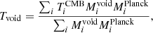
In order to calculate the mean CMB temperature in voids, we defined a set of void weight maps, Mivoid. In these maps, each pixel, i, has a weight in the range of [0.0, 1.0] depending on the number of times the index of the pixel was identified as being inside a projected void in the different void finding procedures. The weight maps thereby take into account the uncertainty in position and size of the voids. The higher the weight, the higher the probability that the pixel is indeed located in a void. Below we describe in detail how these void weight maps were constructed from the different void finding algorithms. When calculating the mean CMB temperature in voids, we took a weighted mean temperature using these void weight maps. We defined the void temperature as
 (1)
(1)
where TiCMB is the CMB temperature in HEALPix4 pixel i (as discussed below, this is often replaced by the temperature of the wavelet-transformed CMB map), Mivoid is the void weight map in pixel i, and MiPlanck is the Planck common mask for pixel i, excluding the parts of the sky where the CMB temperature is uncertain.
The angular radius of the nearby voids that we used in our analysis varies between ∼6° to about ∼30° with a median of about ∼10°. Using the full angular extension of these voids to create the void weight maps, most projected void areas overlap with neighbouring voids and a substantial fraction of the full sky would be used for calculating the mean temperature. We needed to reduce the fraction of the void radii used to create the void maps in order to focus the void temperature measurement on their central parts, seeking a balance between not covering too much area and maintaining sufficient statistics at the same time. We did not know the expected temperature profile in the voids, but still expected a peak towards the centre where the photons had spent a larger time in an underdense environment. We therefore used 1/4, 1/2, and 3/4 of the void radius and created a corresponding void weight map and thereby a void temperature for each of these fractions of the radius.
The typical angular extension of the voids in our redshift range is ∼10°. We therefore expect a possible ISW imprint of these voids to give rise to fluctuations in the CMB at a similar angular scale. Fluctuations at much smaller or larger angular scales then act as noise when trying to identify these void imprints in the CMB fluctuation field. In order to remove these fluctuations at scales outside of the expected angular size of a possible ISW effect, we applied a wavelet transformation to the CMB map before measuring the void temperature. We used the spherical Mexican hat wavelets (Martínez-González et al. 2002, SMHWs), which have strong localization properties on the sphere (and less so in harmonic space), which is important for identifying focused void imprints in their correct positions. The median angular scale of ∼10° of our void sample corresponds to a SMHW wavelet scale of 4° (Vielva et al. 2004). All the void temperatures are based on this wavelet scale, unless otherwise stated. We also tested the robustness of our results with slightly smaller or larger scales, and used the original temperature map for profile calculations.
Another reason for choosing the SMHW is their symmetric shape. Depending on the identification criteria used, the voids may have different shapes (Colberg et al. 2008 and Paillas et al. 2018), but on average they are well described as spherical volumes (Sheth & van de Weygaert 2004; Demchenko et al. 2016, and Wojtak et al. 2016). Furthermore, one of the two algorithms that we used for identifying voids (SPARKLING, see details below) assumes voids to be regions with a spherical shape. A radially symmetric wavelet transform such as the SMHW amplifies such fluctuations.
We further compared the void temperatures with the temperatures previously measured in galactic halos. For CMB temperatures around galactic halos, unless otherwise stated, we used the sample described in H2025 based on large, late-type spiral galaxies in the redshift range 0.004 < z < 0.02 in the three areas with the most massive nearby cosmic filaments. From here on, we use the term ‘galaxy temperature’ to denote the mean temperature of CMB fluctuations taken over these galactic halos. Note that for all galaxy temperature estimates, we always removed the first five multipoles of the CMB map to increase the signal-to-noise ratio, as detailed in H2025.
2.3. Void finding algorithms and void weight maps
As described above, we estimated the mean CMB temperature in voids by calculating the weighted mean of the temperature over the CMB map (or wavelet-transformed map), using the void weight maps to upweight the pixels that had frequently been flagged as belonging to a void. We now explain in detail how voids were identified and how the void weight maps were constructed from the two different void finding algorithms, SPARKLING and REVOLVER.
2.3.1. SPARKLING
The voids were identified with the public void finder SPARKLING5 Ruiz et al. (2015) and Ruiz et al. (2019)) using as tracers (1) all 2MRS galaxies up to z = 0.03 and (2) those with absolute K-band magnitudes MK < −23.93, which constitute a volume-limited sample at z = 0.03 assuming h = 0.674. We included the volume-limited sample, since this assures a constant density of tracers at different redshifts, but at the cost of a smaller density of tracers at lower redshifts. Briefly, the void identification procedure started with an estimation of the galaxy density field via a Voronoi tessellation, which was used to quickly find the underdense regions of the catalogue. Centred in those underdense regions, void candidates were identified as spherical regions with an integrated density contrast satisfying Δ(Rvoid)< − 0.9, Rvoid being the void radius, which means that voids contains only 10% of the density of tracers. Once a void candidate was identified, the computation of Δ was repeated starting from a randomly displaced centre, sampling in this way the volume of the corresponding sphere associated with the initial Voronoi cell and updating the void centre only if the new radius was larger than the previous one. This iterative re-centring procedure guarantee that void centres are located as close as possible to the local minima of the density field. The final step in the identification was a cleaning procedure retaining only the largest non-overlapping voids, while removing the smallest ones.
The stochastic nature of the re-centring process means that different runs with different random seeds produce slightly different results in void centres and radii, depending on whether all galaxies or only the volume-limited sample were used as tracers. In general, the volume-limited sample shows much larger variation with random seeds and is therefore slightly less reliable. In order to construct a map of stable void regions, we created 100 realizations of both sets of tracers, resulting in 200 sets of voids. Among those 200 sets, the void centres and void radii were similar, but some variation was observed. Each pixel in our final void map was then weighted by the number of times the given pixel was flagged as part of a void in those 200 sets. In this way, the void weight map takes into account the uncertainty in void position and radius. The weighted void maps are shown in the left panels of Figure 1.
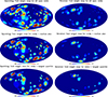 |
Fig. 1. Void weight maps. Left panels: Based on 200 void maps created from SPARKLING combining 100 realizations for the volume-limited sample of galaxies and 100 realizations from the sample using all galaxies. Right panels: Based on Revolver voids identified in the sample using all tracers as well as in the volume-limited sample. Each pixel represents a weight proportional to how many times that pixel was flagged as belonging to a void among those 200 void maps (SPARKLING) or among overlapping voids (REVOLVER). In these maps, a pixel was defined as belonging to a void when it was found within r < 0.5Rvoid for voids identified in the redshift range z = [0, 0.03] based on the 2MRS redshift catalogue. The upper panels show the result when all open voids were included, the middle panels for all voids larger than the median size of a given void set, and the lower panels for the largest quartile of voids. Similar void maps (not shown) were created using only pixels within r < 0.25Rvoid and r < 0.75Rvoid. |
We identified a total number of 192 ± 5 voids (110 ± 3 voids in the volume-limited sample) in this redshift range among each of the 100 sets. The number of voids is clearly much smaller than the number of galaxies, giving considerably poorer statistics in this case. We further expect an RS-like effect to be much stronger for larger voids (in the same way as we found that larger galaxies give rise to stronger cooling (Luparello et al. 2023 and Hansen et al. 2023)). We therefore made two samples and looked at the voids with a void radius larger than the median size of the sample (varying between the 200 sets, but typically Rvoid > 13 Mpc) and the voids of the largest quartile of the sample (typically Rvoid > 17 Mpc). We only considered voids for which the mean integrated density contrast out to 2–3 void radii, Δ23 < 0 (defined as the maximum value of the integrated density contrast between 2 and 3 void radii), is negative, meaning that the voids are surrounded by an underdense region (in the following, we call these ‘open voids’) and not by a shell of matter. We know that the latter voids may be shrinking in contrast to the open voids, which are normally expanding during non-linear growth of perturbations (Sheth & van de Weygaert 2004; Ceccarelli et al. 2013, and Paz et al. 2013). The total number of open voids is 69 ± 4 (40 ± 3 in the volume-limited sample). The weighted void maps limited to these larger voids (median and quartile) are also seen in Figure 1. In the following, we calculated the void temperatures (Equation (1)) using the void weight maps for all the combinations of fractions of void radius (1/4, 1/2, or 3/4 void radius) and for the sample of all the open voids, all the voids larger than the median void radius or all the voids belonging to the largest quartile of void radii.
As a further test of consistency, we also identified open voids where the low-density region outside the void is directed along the line of sight (LOS), meaning that the CMB photons travelling through these voids spend more time in a low-density area. If our working hypothesis involving an anomalous ISW or RS effect holds, we would expect an enhanced positive temperature from these voids. On the other hand, with a standard ISW effect based on a cosmological constant, we would expect these voids to be colder. In the same way that we calculate Δ23, we now define a LOS integrated overdensity, ΔLOS, by considering only the galaxies that are between 1 and 3Rvoid in front of and behind the void, confined to the solid angle defined by the LOS and the radius of the void, as we show schematically in Fig. 2.
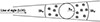 |
Fig. 2. Definition of ΔLOS considering the density within the solid angle subtended by the void between 1 and 3Rvoid. |
2.3.2. REVOLVER
As different void finders and algorithm use different definitions of voids and therefore commonly may identify quite different regions of the sky as voids Colberg et al. (2008) and Paillas et al. (2018)), we also used REVOLVER6 (Nadathur et al. 2019) as an alternative method. This void finder starts with density field computed using a cloud-in-cell algorithm to assign galaxy positions to a regular 3D grid. Once the density field is estimated, a watershed algorithm is used to identify the underdense regions, selecting the density minima as potential void centres. As the void’s boundaries are defined by the crests of the density field, this algorithm identify voids with irregular shapes.
Applying REVOLVER to the same two samples of galaxies, we find 115 voids when using all galaxies and 65 voids when using the volume-limited sample. We defined void radii in a similar way as for SPARKLING, requiring Δ(Rvoid)< − 0.9 around all void centres identified by REVOLVER, ensuring a very low-density region within the void. We find a median void radius of 15 Mpc, similar to the voids identified by SPARKLING. In the right panels of Figure 1, we show the REVOLVER void weight maps side by side with the corresponding SPARKLING maps. For REVOLVER, the voids overlap to a much larger degree than for SPARKLING and high weights indicate pixels where several voids overlap (note that for REVOLVER, there is no random process in the identification of the voids and the weights are therefore a result only of overlapping voids from one single void map and not overlapping voids from different sets of voids). A pixel with a high weight means that this pixel was part of several voids identified by REVOLVER in both galaxy samples (volume-limited and all galaxies). Comparing to the SPARKLING void maps in the left panels, we can see that some regions of the sky are identified as voids by both methods, whereas others are identified by only one method depending on the morphology of the density distribution in the given region. Note also that since a large part of the REVOLVER voids are overlapping, the total sky area occupied by REVOLVER voids is substantially less than for SPARKLING. Therefore, results based only on REVOLVER voids alone (see appendix) have a larger uncertainty.
2.3.3. Combining algorithms
While we test the robustness of our results using the SPARKLING void map and REVOLVER void map separately (see appendix), the main results are presented by the mean of these two voids maps: the pixels of these void maps represent the number of times the given pixel was flagged as being part of a void in SPARKLING and in REVOLVER. A pixel weight larger than 0.5 indicates that the pixel has been part of a void a considerable number of times in both REVOLVER and SPARKLING. A weight of 1 means that the pixel was identified as belonging to a void for all random realization of SPARKLING and that REVOLVER identified several voids overlapping the given pixel. This pixel thus has a very high probability of being in a low-density region. These combined void maps are shown in Figure 3. In addition to giving weight to the mean CMB temperature calculations in voids, the void weight maps were used to create temperature profiles around voids where only voids with high (> 0.5) central weights were used for profile calculations.
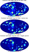 |
Fig. 3. Combined weight maps created from the mean between the REVOLVER void maps and the SPARKLING void maps in Figure 1. The more times a pixel has been flagged as belonging to a void in SPARKLING and REVOLVER, the higher the pixel weight. A weight larger than 0.5 indicates that the pixel has been flagged as a void several times in both methods. From upper to lower panels, the void weight map based on: all open voids, the largest half of the voids, and the larger quartile of voids. |
2.4. Mock galaxy catalogues
In addition to measuring the void weighted CMB temperature in the Planck data and comparing it with the mean temperature in simulated CMB maps using the same void weightings, we also tested our results taking the opposite approach: we applied SPARKLING to 100 mock catalogues of galaxies, created the corresponding 100 void weight maps from each of these mock catalogues, and measured the mean temperature in the Planck CMB map using these 100 void weight maps, comparing it with the temperature obtained using the void weight map from the actual 2MRS survey. Mock galaxy catalogues were constructed by extracting random spherical volumes of radius ∼120 Mpc from the MultiDark Planck 2 (MDPL2) catalogue (Klypin et al. 2016), chosen to match the observational volume of the 2MRS survey. We used the z = 0 snapshot, publicly available through the CosmoSim database7. We increased the radius of the voids in the mocks by a factor of 1.15 such that the median radius of the mock void sample coincides with the median size of the real 2MRS voids to take into account a small difference in the mean density of tracers in the mock and the data.
Note that we have not generated random realizations of the void distribution for each of these 100 mocks, such that the void weight maps for these 100 SPARKLING sets of voids are similar to the ones obtained for REVOLVER: a high pixel weight means that there are many voids overlapping at the given pixel. For the actual 2MRS data however, we do have 100 random realizations, and we created one void weight map for each of these in exactly the same manner as we created the void weight maps for the mock catalogues. In this way, we can compare the 100 mean temperatures obtain on Planck data for each of the 100 mocks as well as for the 100 random realizations of SPARKLING voids for the actual 2MRS data.
2.5. Correlations between galaxy and void temperatures
A main worry when measuring the void temperature in Planck data, where we already know that the CMB temperature around galaxies is much colder than expected, is a possible anticorrelation between the temperature measured in voids and the temperature measured around galaxies. Voids are generally in a part of the sky where there are few galaxies and cold galaxy temperatures could therefore increase the possibility of hot void temperatures. In the results, we show that such an anticorrelation does indeed exist in simulated maps with a quadrupole present. Removing the quadrupole, the anticorrelation is reduced to 2 − 5% depending on the void sample used. We therefore always removed the quadrupole estimated outside the Planck common mask from Planck data and all simulated CMB maps. The quadrupole was estimated inverting the coupling matrix of the aℓm coefficients as described in detail in H2025.
3. Results
In Figure 4 we show the SMICA Planck CMB temperature map masked in such a way that only the areas with galaxies and voids are clearly shown. For the galaxies, discs of 1 Mpc around each galaxy are shown, whereas for the voids the discs correspond to half the void radius. Note that we have taken one realization of the SPARKLING voids here as an illustration. It is clearly visible by eye that the areas around galaxies are cold, whereas the voids on average are warm. Note in particular the prominent hot spot on the right-hand side, just below the galactic mask. This spot was noted already in Marcos-Caballero et al. (2017), where the five most prominent peaks in the CMB were identified. Among these, there are three cold spots, all coinciding with areas of high galactic density seen in the upper panel of Figure 4 and two hot spots, where one is the prominent hot spot seen in the lower panel. The void corresponding to this hot spot is one of the largest voids in the nearby Universe, with a void radius of 22 Mpc situated at z = 0.021. Its position is (l = 263.0° ,b = −19.6° ), while the position of the CMB hot spot in wavelet space is (l = 264.1° ,b = −19.7° ), a distance of 1.1° apart. As a counterpart, in Garcia Lambas et al. (2024), we found a significant coincidence between the CMB Cold Spot (Vielva et al. 2004) and the largest local supergroup, the Eridanus group. This large region shows signs of infalling dynamics as revealed by the large fraction of HI-deficient late-type galaxies.
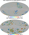 |
Fig. 4. Planck SMICA CMB temperature fluctuation map, masked such that only the areas around nearby galaxies (upper panel) and voids (lower panel) are clearly visible. The mask consists of holes of 1 Mpc radius around all large nearby spiral galaxies in the most massive galactic filaments within z < 0.02 (see H2025 for details). The void holes includes one realization of SPARKLING voids, including all voids with Δ23 < 0 out to z < 0.03 and extend to 1/2 void radius. The full CMB temperature map can be seen in the background. It can clearly be seen that the CMB temperature is mostly negative around galaxies and mostly positive in voids. |
We measured the weighted mean temperature over all the voids in the data as well as in 10 000 SMICA simulations. In Table 1 we show the mean temperature for the data measured in terms of standard deviations estimated from simulations. We see that the CMB temperature in voids is significantly warmer than expected in simulations and that the mean temperature increases with the void size, reaching 3.5σ for the largest voids. We see that already using all open voids, regardless of size, the mean temperature is always ≥2σ. The significances then gradually increase with void size, as would be expected if an ISW or RS-like effect were at play. The signal is not a result of a few very hot voids, but is rather driven by a trend whereby the larger voids generally are warmer. This can be seen in Figure 5, where we show the mean temperature within 0.5Rvoid of each void, including only voids with weights larger than 0.5 in Figure 3 and that therefore have a higher probability of belonging to an actual void. In the figure, which is limited to the voids in the largest quartile, we can see that almost all voids have a positive temperature.
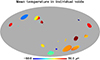 |
Fig. 5. Mean CMB temperature within 0.5Rvoid of each individual void for voids within the largest quartile. Voids are taken from the combined Sparkling sample, where only voids appearing in > 50% of the random realizations are included, corresponding to the voids that have the largest weights in the void weight maps of Figure 1. The fact that the void position and radius differ slightly for different realizations is reflected in the varying temperature within one single void for some of the voids. |
Significances of void temperatures on wavelet-transformed SMICA maps (with quadrupole removed).
To test consistency, in Table 1, we also show the corresponding significances for other wavelet scales and radii showing generally consistent results. In Table 2 we show the same results using only the voids with ΔLOS < 0 having an extended underdense region along the LOS around the void. We see clearly that these voids show higher significances, reaching 4σ for the largest voids. Note further that all significance values here are taken with respect to a zero expectation value. In the Λ cold dark matter (ΛCDM) model, the expected void temperatures given the standard ISW effect, is negative and about −4 μK (judging from Figure 1 in Cai et al. (2010) taken from a simulated slab of 100h−1Mpc at z = 0) while we, on the contrary, have detect a large positive temperature. Therefore, comparing to the standard cosmological constant scenario, the actual significance of the deviation is even larger than the significances quoted here.
Significances of void temperatures on wavelet-transformed SMICA maps (with quadrupole removed) using only voids with negative density along the LOS, ΔLOS < 0.
Figure 6 shows a detailed mean temperature profile. Note that this profile was obtained from the original CMB temperature map and not from the wavelet-transformed map. We can see that the temperature goes to zero at a distance of about one void radius. The temperature profile in large voids in Figure 6 shows that the inner parts of these voids have a mean temperature of about ∼30 − 40 μK, similar to the ∼ − 27 μK galaxy temperatures reported in H2025. In Figure 7, we show the variance-weighted temperature difference between the first bin of this temperature profile of the voids (for the largest quartile of voids) and the mean galaxy temperature for large spiral galaxies in massive filaments. The observed temperature difference of 69 μK is not found in any of the 10 000 simulated maps. Indeed the temperature difference observed in the data is more than 40% larger than the largest difference found in simulations. A Gaussian fit to the temperature differences is drawn as a red line in the figure and shows that the distribution is close to Gaussian. As an approximate measure of significance, assuming a nearly Gaussian distribution, the temperature difference in the data is 6.5σ larger than expected. Note again that we have compared this difference of 6.5σ to a zero expectation value, whereas we should have compared to the expectation given by the standard ΛCDM model giving a negative difference of about −8 μK (judging again from Figure 1 in Cai et al. (2010) where voids appear to have a temperature of ∼ − 4 μK and overdensities about ∼4 μK giving 8 μK difference), which gives an even larger tension with the standard model based on a cosmological constant.
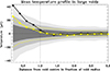 |
Fig. 6. Mean CMB temperature in radial bins around voids: the black line shows the temperature taken from the largest quartile and the yellow line the one from all open nearby voids in the Planck SMICA CMB temperature fluctuation map with the quadrupole removed. Each bin is taken as 1/5 of the void radius. The grey bands show the 67%, 95%, and 99.7% confidence intervals based on 10 000 simulated maps for the largest quartile of voids and the dashed yellow line shows the corresponding 95% interval for the sample of all voids. Note that the profiles are only taken around voids with a central weight of > 0.5 in the void weight map (Figure 3), ensuring that the voids used for measuring the profile are flagged as a void in most random realizations of SPARKLING as well as in REVOLVER. |
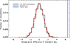 |
Fig. 7. Variance-weighted temperature difference between the mean CMB temperature in voids (inner temperature profile bin of the largest quartile of voids from Fig. 6) and the mean CMB temperature around galaxies (from H2025). The histogram shows the temperature difference in 10 000 SMICA simulations in terms of standard deviations calibrated on simulations. The red curve shows a Gaussian fit to the histogram. The blue line shows the corresponding difference in the data. |
4. Discussion
Based on the findings of H2025 in which CMB temperatures are significantly colder around nearby galactic halos than expected in the standard ΛCDM model, we put forward the hypothesis that recent changes in the gravitational potential evolution give rise to a negative ISW effect. Such a hypothesis predicts that not only are the CMB photons passing through overdensities cooled, but CMB photons passing through underdensities would be heated. We tested the hypothesis by measuring the mean temperature of the CMB temperature as measured by the Planck satellite in all nearby voids. We have shown that the mean CMB temperature in these voids is indeed larger than expected at the 2 − 4σ level depending on the void size, fraction of the void, and LOS densities around the void. If the ISW hypothesis were correct, one would expect an increasing signal for (1) increasing void sizes and (2) for voids with underdense global environment, particularly when these low-density surroundings are elongated along the LOS making the photon path inside an underdense environment longer. We have shown that both of these properties are seen in the data. We further estimate the temperature difference between the mean temperature around galactic halos and the mean temperature in voids and find a temperature difference that is ∼6.5σ larger in the data compared to 10 000 simulated maps, assuming a Gaussian distribution of temperature differences in simulations. We now discuss several aspects of the statistics used and the reliability of the results.
4.1. Look-elsewhere effect
The importance of correcting for the impact of the number of choices made in the analysis is particularly important for serendipitous discoveries such as the cooling of CMB photons around galaxies described in L2023 and followed up in H2025. In the latter paper, a thorough analysis and correction for the look-elsewhere effect was performed and it was shown that even when taking all choices into account, the significance was still at the p < 0.0001 level.
The discovery of warmer CMB temperature in nearby voids described in this paper was not serendipitous. Based on our previous findings, we made the conjecture that the observed cooling of CMB photons in nearby galaxies could have a possible origin in an anomalous ISW or RS effect. This conjecture was based on the fact that the frequency independence of the effect is difficult to explain in terms of other known mechanisms. In the lack of alternative explanations, we here test if an altered ISW or RS effect may cause the observed cooling.
Assuming this is indeed the case, we would expect a priori, based on what we know about ISW or RS effects:
-
that voids in the same redshift range as the galaxies for which cooling is observed, and particularly open voids, which we expect to be expanding, and hence having an opposite change of potential than the contracting galactic filaments, would be warmer than expected for a standard model CMB sky.
-
that the central parts of the voids are warmer and gradually decreasing towards a mean temperature of zero outside of the void radius.
-
that the larger voids would be warmer than the smaller voids.
-
that voids with a surrounding underdense region elongated along the LOS (ΔLOS < 0) would produce a stronger effect.
These expectations strongly limit the number of choices that it is possible to make when analysing the voids. Many of the choices made in this analysis could not have been very different due to these expectations. These are not parameters that can be fine-tuned to make a significant detection as we assume a possible physical mechanism, limiting these choices.
We nevertheless corrected for the look-elsewhere effect and for the different choices made for the case where there is indeed a possible range of parameters to adjust. The choices made in the analysis can be listed as
-
The redshift range: The cooling in galactic filaments has been observed for z < 0.04 (H2025, DF2025), within which the 2MRS galaxy catalogue allows for the reliable identification of filaments. The identification of voids needs a sufficient number density of tracers in order to obtain void detections not highly affected by Poisson uncertainties. In this context, the 2MRS catalogue has a fair completeness up to z = 0.03, making the choice of redshift range strongly limited by available data and is not a parameter that we can change. We simply apply our analysis to the largest available volume for each tracer. Nevertheless, in the appendix, we show that the results are consistent when we divide this redshift range into two sub-ranges and analyse void temperatures in each range separately.
-
The choice of spherical Mexican hat wavelets: These wavelets have been the most applied type of symmetric wavelets used in CMB analysis. Their strong localization properties on the sphere Martínez-González et al. (2002) and Scodeller et al. (2011)) are an advantage when searching for localized features on the sky. The wavelet coefficients of the SMHW are equivalent to the curvature of the field smoothed with a Gaussian kernel (Marcos-Caballero et al. 2017) such that the peaks of the SMHW are equal to the peaks in the local curvature of the smoothed CMB. For these reasons the SMHW was the first choice in our work. Given that they were used to discover the CMB cold spot (Vielva et al. 2004) and were used by the Planck team when testing for general deviations from isotropy and Gaussianity in the CMB Planck Collaboration XVI (2016) and Planck Collaboration VII (2020)), we expect the SMHW to be an optimal choice for identifying possible ISW-void-induced fluctuations in the temperature field. Furthermore, due to their strong ability to identify symmetrically shaped features, they were also shown optimal for identifying extragalactic point sources in CMB data (Gonzalez-Nuevo et al. 2006) and were the basis for the Planck point source catalogue (Planck Collaboration XXVI 2016). Note that in the latter work, the MHW2 family of wavelets was used. We repeated our calculations with the version of MHW2 adapted to the sphere, the SMHW2 wavelets used for instance for point source detection in the CBASS survey (Grumitt et al. 2020), and found slightly stronger void temperature significances than with the standard SMHW. Another class of wavelets used extensively in CMB analysis is the needlet class of wavelets (Narcowich et al. 2006 and Pietrobon et al. 2006), used for instance for the NILC component separation method for Planck data (Delabrouille et al. 2009). The standard needlets have excellent localization properties in harmonic space, but less so in real space, which is needed for our work (Scodeller et al. 2011). However, the Mexican needlets (Geller & Mayeli 2008), also used for the MC-NILC component separation (Carones et al. 2023), have stronger localization properties in real space, but the wavelet kernel for Mexican needlets is almost identical to the SMHW kernel (Scodeller et al. 2011) and we therefore expect almost identical results.
-
Using open voids: This was already explained above. Open voids are expected to be expanding. Based on our conjecture of a non-standard ISW or RS effect, we would expect to see the effect in expanding voids due to the potential change. The same potential change is therefore not expected in closed voids Sheth & van de Weygaert (2004), Ceccarelli et al. (2013), and Paz et al. (2013)), and we therefore only analyse open voids in this work.
-
The choice of a wavelet scale of 4 degrees: As explained in detail above, the median radius of the voids in our sample is 10°, corresponding to a SMHW scale of 4°. Most voids therefore have an angular extension around this scale and is therefore a natural first choice. But in order to test the robustness of this wavelet choice, also for smaller and larger voids, we chose to look at the nearest scale below and above the median size. We therefore also list results for 3° and 5° scales and we account for the three possible choices of scales when correcting for the look-elsewhere effect.
-
The choice of void size samples. We have chosen to look at (1) all open voids, (2) only the largest half of the voids, and (3) only the largest quartile of voids. Based again on our assumption about an ISW or RS-like effect, we expect a larger signal in larger voids. The first natural choice is therefore to look at the largest half. Finally, in order to study even larger voids, we divide the largest half again in two, looking therefore also at the largest quartile of void sizes. We correct for the look-elsewhere effect by looking at these three choices of samples in simulations.
-
The fraction of the void radius used to measure temperature: Assuming an ISW effect, we would expect the CMB temperature to be hotter in the centre of the void and gradually decrease towards the edges. As a first natural choice, we used half of the void radius to measure the temperature. A smaller fraction of the void radius gives less statistics and a larger fraction would dilute the signal, including parts of the void where we expect less heating of the CMB photons. To test the stability of the results, however, we also divided these ranges in two and measured the inner 1/4 of the voids as well as including 3/4 of the void radius. We corrected for the look-elsewhere effect for these three choices.
In Table 1, we can see the significances of our detection for all the choices which have been made. We calculated the significance for all of the same choices in all simulations, giving a similar table for each of the 9000 simulated CMB maps (1000 simulations are used for obtaining standard deviations). The problem of the look-elsewhere effect is the fact that the significance we find varies depending on the which of the numbers in the table we choose. We bypassed this problem in two different ways:
-
By taking the maximum value over the significances in the table for each single simulation. For each simulation individually, we find the optimal combination of these parameters that maximizes the detection level for that given simulation. This detection level (measured in number of standard deviations) is then recorded. In Figure 8 we show a histogram of this maximum detection level for each simulation. The vertical line shows the same number for the actual data. Only 0.2% of 9000 simulations have a higher maximum detection level.
-
By taking the mean value over the significances in the table for each single simulation. Clearly statistical fluctuations may show a high detection level in some simulated maps, given a sufficient number of simulations. However, for a real stable detection, we would expect most of the numbers in the table to be high, since the expected size of the voids varies within the given wavelet scales tested and since a real effect would show some significance for several size samples and not just one sample. We therefore also take the mean over all significances in the table for each simulation. In Figure 8 we show this mean value for each simulation. We see again that only 0.2% of the simulations show a similar or higher mean detection level (about half of these simulations are among the 0.2% that also have a higher maximum detection). This shows that it is highly uncommon in a simulation to find both such a high maximum detection level as we find in the data and a high detection level that is equally stable as in the data. We see in the same figure that when imposing ΔLOS < 0, the number of simulations with a similarly high maximum and mean detection level is even smaller.
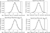 |
Fig. 8. Histograms showing the maximum detection level for void temperatures (upper left panel; 0.2% of the simulations have a higher maximum detection level), the mean detection level for void temperatures (upper right panel; 0.2% of the simulations have a higher mean detection level), the maximum detection level for void temperatures using only voids with ΔLOS < 0 (lower left panel; 0.03% of the simulations have a higher maximum detection level), and the mean detection level for void temperatures using only voids with ΔLOS < 0 (lower right panel; 0.09% of the simulations have a higher mean detection level). All cases are based on 9000 simulations and the free parameters (void size, wavelet scale, and the ratio of the void radius) are either varied to optimize the detection for each simulation (for maximum detection) or the significances are averaged over the parameter values in Table 1 (mean detection). The vertical lines show the same number for the real data. |
4.2. Void temperatures in mock catalogues
We repeated the above-described procedure for 100 mock void maps measuring the void temperature for Planck data for each mock with significances calibrated on void temperatures from CMB simulations for each individual mock void weight map. For each mock, we then created a table similar to Table 1 including the significance values for the same combinations of void sizes, radius fractions, and wavelet scales, and from this table we created the maximum and mean detection level, similar to Fig. 8, for each mock. In Figure 9, we compare these to the numbers obtained in the same manner for 100 realization of the SPARKLING voids in 2MRS data. We can see that the maximum significances are higher in all 100 realizations of the observed voids than in any of the 100 mocks void sets, confirming our previous results.
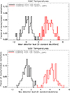 |
Fig. 9. Mean (upper panel) and maximum (lower panel) detection levels in mocks (black histogram) and in 100 realizations of 2MRS voids. In the same way as in Fig. 8, we calculated the mean and maximum detection levels taken over the different parameter variations shown in Table 1 for the void sets of each individual mock catalogue and for 100 SPARKLING void realizations based on 2MRS data. All temperatures were calculated on the actual Planck SMICA CMB map and significances calibrated on the corresponding CMB simulations. |
4.3. Dependence on CMB frequency map, cleaning process, and Planck data release
In Figure 10, we show the mean detection level, estimated in the same manner as in Figure 8, but using different CMB maps. We have chosen to focus on the sample of voids giving the strongest detection, the voids with ΔLOS < 0, and to test the robustness of the significance for this case. The black histogram again shows the SMICA component separation algorithm results from the Planck PR3 data release already shown in the lower right panel of Figure 8, but now using the CMB map based on the SMICA algorithm optimized on the removal of the Sunyaev-Zeldovich (SZ) effect from the data.
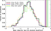 |
Fig. 10. Histogram showing the mean detection level for void temperatures over the free parameters (void size, wavelet scale, and ratio of void radius) for each of our 1000 simulations using only voids with ΔLOS < 0. The vertical line shows the same number for the real data. Results are shown for the Smica NO-SZ map where contamination from the SZ effect has been removed, the SEVEM cleaned frequency bands at 100GHz and 217GHz, the WMAP cleaned Q-band at 41Ghz, and the SEVEM cleaned map from the last PR4 Planck release. |
The green histogram shows the corresponding results for the CMB map obtained from the SEVEM component separation algorithm for the newer Planck PR4 data release. Note, however, the much higher uncertainty for this result, as only 600 simulated maps were produced for PR4 as opposed to the 10 000 SMICA maps in PR3. The remaining three histograms show the maps obtained from the individual 100 GHz and 217 GHz Planck channels using the SEVEM component separation method as well as the WMAP 41 GHz channel. Note that the beam size, noise level, and foreground residual level are different in these different maps, giving rise to different histograms. In particular, the WMAP 41 GHz channel has a much larger beam and noise level than the Planck maps, giving rise to a broader histogram.
We also analysed the void temperatures for the CMB maps created from the NILC and Commander component separation algorithms, using 1000 simulations of each. We found for both sets of maps that none of the 1000 simulated maps have a similarly high maximum or mean detection level as the data, consistent with the above results for SMICA and SEVEM. We see that for all these different cases, the significance of the results remains similar and robust.
4.4. Possible temperature anticorrelations between areas of filaments and voids
In the introduction, we already mentioned our worry about a possible expected anticorrelation between galaxy temperatures and void temperatures. Due to the large-scale fluctuations of the CMB, a simulation that by coincidence (or by a physical process) exhibits cold galaxy temperatures could have a higher probability of having hot void temperatures. The reason for this is more easily seen in Figure 4. There is little overlap between the parts of the sky occupied by the nearby galactic filaments (upper panel) and the parts of the sky occupied by the nearby voids (lower panel). In order to keep the mean temperature over the full sky zero while the CMB around galaxies is cold, the void areas need to be hot, creating a quadrupolar structure that would be evident if one combined the two panels of the figure. We show that this quadrupole indeed introduces a strong anticorrelation and that by removing the quadrupole from simulated CMB maps (and from the actual data) this anticorrelation is strongly reduced.
In order to test the presence of such an anticorrelation, we look at the outliers of the simulations: among our 10 000 simulated CMB maps, we chose the 100 simulations with the coldest galaxy temperature. If an anticorrelation were present, we would expect the void temperatures for these simulations to be warm and vice versa. For the main galaxy sample of H2025, there is no CMB simulation that exhibits a galaxy temperature as cold as in the real data. We therefore chose to look at the sample of all large spiral galaxies and not only those in the massive galactic filaments that are the ones giving the strongest detection. In this case, 15 of the 10 000 simulated CMB maps have a galaxy temperature colder than in the data. Using this sample, it is easier to compare with actual data: we checked whether simulated CMB maps with galaxy temperatures which are even colder than in the data also show void temperatures as hot as, or hotter than, in the data.
In Figure 11 we show the void temperatures of the 100 CMB simulations that exhibit the coldest galaxy temperatures and the 100 CMB simulations that exhibit the hottest ones. The upper panel shows results without removing the quadrupole and the lower panel shows the results with the quadrupole removed. We can clearly see that in the case in which the quadrupole is maintained, the simulations with cold galaxy temperatures show hotter void temperatures and vice versa. There is even one of the cold galaxy simulations with a hotter void temperature that in the data. When the quadrupole is removed, as expected, this trend is almost completely removed. The histograms are superposed and one can even see that the largest tail of the simulations with cold galaxy temperatures also show cold, not hot, void temperatures.
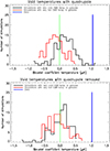 |
Fig. 11. Void wavelet temperatures of voids with Rvoid within the largest quartile in 100 simulated CMB maps without (upper panel) and with (lower panel) the quadrupole removed. Black histograms show the void temperatures of the 100 simulations (of 10 000) with the coldest mean CMB temperature around galaxies and red histograms show the 100 simulations with the hottest temperature around galaxies. Blue line show the void temperature in Planck data. The histogram is shown with very small bins such that individual simulations are visible. |
Measuring the correlation coefficient between galaxy and void temperatures for the largest quartile of voids while keeping the quadrupole, we find an anticorrelation of 10%–30% depending on the fraction of void radius used. After removing the quadrupole, this anticorrelation is reduced to between 2% and 5%. These tests show the importance of removing the quadrupole from the CMB simulations before testing galaxy and void temperatures. We see from Figure 11 that the small anticorrelation remaining after subtracting the quadrupole is unable to account for the high void temperatures found in the data.
5. Conclusions
We have found that CMB photons passing through nearby voids are significantly hotter than expected, whereas CMB photons passing through the overdensities in the nearby galactic halos are correspondingly colder than in simulations (see Figure 4 for an illustration). Our results show the opposite of the predicted ISW effect in the local Universe (Cai et al. 2010) due to a cosmological constant, but consistent with what one would observe if an unknown mechanism makes the gravitational potentials in the recent Universe (z ≲ 0.1) increase, causing a negative ISW effect. An independent confirmation of our results was reported in Davies et al. (2025), in which they confirm this sign change of the ISW effect at low redshift using low-density cylinders elongated along the LOS, cosmic tunnels, instead of voids.
Recent results from DESI (DESI Collaboration 2025; Lodha et al. 2025) show evidence for dynamical dark energy and possible phantom crossing at higher z. In Son et al. (2025), supernova data were corrected for progenitor age bias, giving strong evidence for dynamical dark energy and a non-accelerating Universe at low redshift, and thereby again opening the possibility for a gravitational potential evolution and ISW effect in the nearby Universe that is not consistent with the standard ΛCDM prediction.
At high redshifts (z ≳ 0.1) the positive ISW effect consistent with a cosmological constant has been detected at the 3 − 4σ level, but with several reports of a significant excess in some datasets and redshift ranges (Szapudi 2025). In Francis & Peacock (2010) the correlation between the integrated projected mass density from 2MASS in the redshift range z = [0, 0.1] using photometric redshifts and WMAP CMB data was found to be within the expectation for the ISW effect at the largest scales. The main difference from our work is the use of photometric redshifts instead of the spectroscopic redshifts, the focus on much larger angular scales and that they average over a much larger redshift range than in this work. Note further Kovács et al. (2022), in which a negative ISW effect is also claimed for z > 1.5.
The DESI results seem to indicate that the properties and evolution of the dark energy may be poorly understood. One cannot exclude that unknown properties of dark energy could give rise to strongly increasing gravitational potentials at small redshifts. An example of a theory that predicts such a behaviour is given in Hlozek et al. (2015). In that work, ultra-light axions play the role of dark energy at early times and behave similar to dark matter in recent times, thereby increasing the potentials and giving rise to the ISW effect changing sign as shown in their Figure 5. Also, in theories of Galilean gravity such a sign change can occur (Barreira et al. 2014; Renk et al. 2017). Further work is necessary to test whether these theories or a similar mechanism are fully consistent with the observed signal and other cosmological observations.
We have shown that many aspects of our findings are consistent with the expected behaviour of an (inverse) ISW effect: (1) the signal is frequency-independent, (2) the effect increases with increasing void sizes, (3) the rise in temperature is higher in the central parts of the voids and falls to zero at about one void radius, and (4) the effect is stronger in voids with an extended underdense region along the LOS. The results have been shown to be robust to changes in versions of the CMB Planck map, the component separation algorithm, and the Planck frequency used for creating the CMB map. In the appendix, we also show that the results persist when splitting the data into two separate galactic hemispheres, in two different redshift ranges, and when using only SPARKLING or only REVOLVER voids separately. For the voids that have an underdensity along the LOS, if we assume the standard ISW scenario with a cosmological constant, we would expect a lower temperature in these voids and thereby a smaller detection. We find, on the contrary, a larger temperature and a larger detection in these voids compared to other voids. This would be more consistent with an anomalous dark energy and ISW effect where an underdensity increases the CMB temperature.
The amplitude of the ISW effect at higher redshift is normally calculated by cross-correlating the maps of large-scale structure, often represented as maps of galaxy number density, with the CMB fluctuations, assuming linear evolution of density perturbations. Due to the proximity of structures at z < 0.03, such a cross-correlation would require a detailed knowledge of the density field at non-linear scales, since individual galaxies and voids here occupy a substantial number of pixels, often spanning several degrees on the sky. A more accurate comparison with the expected ISW effect is therefore deferred to a future study as it requires one to calculate the ISW effect using a detailed model of the nearby density field.
Acknowledgments
Thanks to Dennis Fremstad, Hans Winther, Farbod Hassani, Abdolali Banihashemi, Prajwal Puttasiddappa and Sigurd K. Næss for discussions and suggestions. Results in this paper are based on observations obtained with Planck (http://www.esa.int/Planck), an ESA science mission with instruments and contributions directly funded by ESA Member States, NASA, and Canada. We acknowledge the use of NASA’s WMAP data from the Legacy Archive for Microwave Background Data Analysis (LAMBDA), part of the High Energy Astrophysics Science Archive Center (HEASARC). The simulations were performed on resources provided by UNINETT Sigma2 – the National Infrastructure for High Performance Computing and Data Storage in Norway. Some of the results in this paper have been derived using the HEALPix package (Górski et al. 2005).
References
- Barreira, A., Li, B., Baugh, C., & Pascoli, S. 2014, JCAP, 08, 059 [Google Scholar]
- Bennett, C. L., Halpern, M., Hinshaw, G., et al. 2003, ApJS, 148, 1 [Google Scholar]
- Cai, Y.-C., Cole, S., Jenkins, A., & Frenk, C. S. 2010, MNRAS, 407, 201 [NASA ADS] [CrossRef] [Google Scholar]
- Carones, A., Migliaccio, M., Puglisi, G., et al. 2023, MNRAS, 525, 3117 [Google Scholar]
- Ceccarelli, L., Paz, D., Lares, M., Padilla, N., & Garcial Lambas, D. 2013, MNRAS, 434, 1435 [NASA ADS] [CrossRef] [Google Scholar]
- Colberg, J. M., Pearce, F., Foster, C., et al. 2008, MNRAS, 387, 993 [Google Scholar]
- Cruz, M., Martínez-González, E., Gimeno-Amo, C., Kavanagh, B. J., & Tucci, M. 2024, ArXiv e-prints [arXiv:2407.17599] [Google Scholar]
- Davies, C. T., Klein, M., Fumagalli, A., & Mohr, J. J. 2025, ArXiv e-prints [arXiv:2510.16799] [Google Scholar]
- Delabrouille, J., Cardoso, J.-F., Le Jeune, M., et al. 2009, A&A, 493, 835 [NASA ADS] [CrossRef] [EDP Sciences] [Google Scholar]
- Demchenko, V., Cai, Y.-C., Heymans, C., & Peacock, J. A. 2016, MNRAS, 463, 512 [Google Scholar]
- DESI Collaboration (Abdul-Karim, M., et al.) 2025, ArXiv e-prints [arxiv:2503.14738] [Google Scholar]
- Dominguez Feldman, J. I., Pereyra, L. A., Hansen, F. K., Toscano, F., & Garcia Lambas, D. 2025, Phys. Rev. D, submitted [arXiv:2506.08833] [Google Scholar]
- Dong, F., Zhang, P., Sun, Z., & Changbom, P. 2023, ApJ, 938, 72 [Google Scholar]
- Francis, C. L., & Peacock, J. A. 2010, MNRAS, 406, 14 [Google Scholar]
- Garcia Lambas, D., Hansen, F. K., Toscano, F., Luparello, H., & Boero, E. F. 2024, A&A, 681, A2 [CrossRef] [EDP Sciences] [Google Scholar]
- Geller, D., & Mayeli, A. 2008, Mathematische Zeitschrift, 262, 895 [Google Scholar]
- Gonzalez-Nuevo, J., Argueso, F., Lopez-Caniego, M., et al. 2006, MNRAS, 369, 1603 [NASA ADS] [CrossRef] [Google Scholar]
- Górski, K. M., Hivon, E., Banday, A. J., et al. 2005, ApJ, 622, 759 [Google Scholar]
- Grumitt, R. D. P., Taylor, A. C., Jew, L., et al. 2020, MNRAS, 496, 1941 [Google Scholar]
- Hansen, F. K., Boero, E. F., Luparello, H. E., & Garcia Lambas, D. 2023, A&A, 675, L7 [NASA ADS] [CrossRef] [EDP Sciences] [Google Scholar]
- Hansen, F. K., Garcia Lambas, D., Luparello, H. E., Toscano, F., & Pereyra, L. A. 2025, A&A, 696, A184 [NASA ADS] [CrossRef] [EDP Sciences] [Google Scholar]
- Hlozek, R., Grin, D., Marsh, D. J. E., & Ferreira, P. G. 2015, Phys. Rev. D, 91, 103512 [NASA ADS] [CrossRef] [Google Scholar]
- Huchra, J. P., Macri, L. M., Masters, K. L., et al. 2012, ApJS, 199, 2 [Google Scholar]
- Kovács, A., Beck, R., Smith, A., et al. 2022, MNRAS, 513, 15 [CrossRef] [Google Scholar]
- Krolewskia, A., & Ferraroc, S. 2022, JCAP, 04, 033 [Google Scholar]
- Klypin, A., Yepes, G., Gottlober, S., Prada, F., & Hess, S. 2016, MNRAS, 457, 4340 [CrossRef] [Google Scholar]
- Lodha, K., Calderon, R., Matthewson, W. L., et al. 2025, Phys. Rev. D, 112, 27 [Google Scholar]
- Luparello, H. E., Boero, E. F., Lares, M., Sánchez, A. G., & Lambas, D. G. 2023, MNRAS, 518, 5643 [Google Scholar]
- Marcos-Caballero, A., Martínez-González, E., & Vielva, P. 2017, JCAP, 05, 023 [Google Scholar]
- Martínez-González, E., Gallegos, J. E., Argüeso, F., Cayón, L., & Sanz, J. L. 2002, MNRAS, 336, 22 [Google Scholar]
- Maturi, M., Dolag, K., Waelkens, A., Springel, V., & Enßlin, T. 2007, A&A, 476, 83 [NASA ADS] [CrossRef] [EDP Sciences] [Google Scholar]
- Nadathur, S., Carter, P. M., Percival, W. J., Winther, H. A., & Bautista, J. E. 2019, Phys. Rev. D, 100, 023504 [CrossRef] [Google Scholar]
- Narcowich, F. J., Petrushev, P., & Ward, J. D. 2006, SIAM J. Math. Anal., 38, 574 [CrossRef] [Google Scholar]
- Paillas, E., Cautum, M., Li, B., et al. 2018, MNRAS, 484, 1149 [Google Scholar]
- Paz, D., Lares, M., Ceccarelli, L., Padilla, N., & Garcia Lambas, D. 2013, MNRAS, 448, 1471 [Google Scholar]
- Pietrobon, D., Balbi, A., & Marinucci, D. 2006, Phys. Rev. D, 74, 043524 [NASA ADS] [CrossRef] [Google Scholar]
- Planck Collaboration XVI. 2016, A&A, 594, A16 [NASA ADS] [CrossRef] [EDP Sciences] [Google Scholar]
- Planck Collaboration XXVI. 2016, A&A, 594, A26 [NASA ADS] [CrossRef] [EDP Sciences] [Google Scholar]
- Planck Collaboration I. 2020, A&A, 641, A1 [NASA ADS] [CrossRef] [EDP Sciences] [Google Scholar]
- Planck Collaboration IV. 2020, A&A, 641, A4 [NASA ADS] [CrossRef] [EDP Sciences] [Google Scholar]
- Planck Collaboration VII. 2020, A&A, 641, A7 [NASA ADS] [CrossRef] [EDP Sciences] [Google Scholar]
- Planck Collaboration LVII. 2020, A&A, 643, A42 [NASA ADS] [CrossRef] [EDP Sciences] [Google Scholar]
- Rees, M. J., & Sciama, D. W. 1968, Nature, 217, 511 [Google Scholar]
- Renk, J., Zumalacárregui, M., Montanari, F., & Barreira, A. 2017, JCAP, 10, 020 [Google Scholar]
- Ruiz, A. N., Paz, D. J., Lares, M., et al. 2015, MNRAS, 448, 1471 [NASA ADS] [CrossRef] [Google Scholar]
- Ruiz, A. N., Alfaro, I. G., & Garcia Lambas, D. 2019, MNRAS, 483, 4070 [NASA ADS] [CrossRef] [Google Scholar]
- Sachs, R. K., & Wolfe, A. M. 1967, ApJ, 147, 73 [NASA ADS] [CrossRef] [Google Scholar]
- Scodeller, S., Rudjord, Ø., Hansen, F. K., Marinucci, D., Geller, D., & Mayeli, A. 2011, ApJ, 733, 2 [NASA ADS] [CrossRef] [Google Scholar]
- Son, J., Lee, Y-W., Chung, C., Park, S., & Cho, H. 2025, MNRAS, 544, 975 [Google Scholar]
- Sheth, K., & van de Weygaert, R. 2004, MNRAS, 350, 517 [NASA ADS] [CrossRef] [Google Scholar]
- Szapudi, I. 2025, Philos. Trans. A Math. Phys. Eng. Sci., 383, 20240026 [Google Scholar]
- Toscano, F., Hansen, F. K., Garcia Lambas, D., et al. 2025, Phys. Rev. D, 111, 083528 [Google Scholar]
- Vielva, P., Martinez-Gonzalez, E., Barreiro, R. B., Sanz, J. L., & Cayon, L. 2004, ApJ, 609, 22 [NASA ADS] [CrossRef] [Google Scholar]
- Wojtak, R., Powell, D., & Abel, T. 2016, MNRAS, 458, 4431 [Google Scholar]
Appendix A: Testing validity of the results on data splits
Here we show detailed results of several data splits. In this way, we can test consistency in a new way: If the observed effect originates form a physical process and not from coincidence, one would expect the observed heating of voids to be present throughout all parts of the data. Here we look at the void temperature results using each void finder algorithm separately, measuring the void temperature in the northern and the southern galactic hemisphere separately and finally measuring the void temperatures in two different redshift shells. Dividing the data in two, there is less data in each part and therefore larger uncertainties, impeding the division of the data in even smaller parts. With larger uncertainties, the distributions from simulations become broader and more simulations spuriously have high values, similar to the data. We therefore expect lower significance values in each independent part of the data. The high significances in the main part of the paper therefore appear as a result of combining data where all parts of the data show similar trends and the combination results in lower uncertainties and higher significances.
We first look at results using SPARKLING and REVOLVER voids separately in Table A.1 and Table A.2. We see that in both cases, although the voids positions and sizes are quite different, we find 2 − 3σ detections. As can be seen in Figure 1, the uncertainty for REVOLVER results are larger given the small area on the sky occupied by the voids. For REVOLVER the significances for the smaller voids are less than 2σ while the larges quartile of voids shows larger significances than the corresponding void sizes for SPARKLING. For SPARKLING, we also see in Table A.3 the general trend that voids with ΔLOS < 0 show higher CMB temperatures. For REVOLVER, most voids satisfy this condition and no significant difference is therefore seen when limiting ΔLOS < 0 for REVOLVER voids (results not shown).
Significances of SPARKLING void temperatures on wavelet-transformed SMICA maps (with quadrupole removed).
Significances of REVOLVER void temperatures on wavelet-transformed SMICA maps (with quadrupole removed).
Significances of SPARKLING void temperatures on wavelet-transformed SMICA maps (with quadrupole removed) using only voids with ΔLOS < 0.
In Figure A.1 and Figure A.2 we show the temperature profiles for SPARKLING and REVOLVER voids respectively. Both sets of voids separately show consistent profiles to the combined case in Figure 6.
In Figure A.3, we show the result of correcting for the look-elsewhere effect for SPARKLING and REVOLVER voids separately. Again we see that both mean and maximum detection levels are in the far tail of the distribution obtained from simulations. For SPARKLING alone, only 0.4% of the simulations have similar og higher mean detection and 0.9% a higher maximum detection. This decreases to 0.1% when limiting to voids within undersensities along the LOS. For REVOLVER with void temperatures which are not significantly high for for smaller voids as can be seen in Table A.2, the maximum and mean detection level when including all numbers in the table are still significant, only 0.2% of the simulations have a similar maximum detection when optimizing parameters for each simulation, and only 0.9% of the simulations have a similar or higher mean detection level.
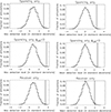 |
Fig. A.3. Same as Figure 8, but for SPARKLING and REVOLVER voids separately. Left column: max values, right column: mean values, upper row: SPARKLING open voids, middle row: SPARKLING voids with ΔLOS < 0, lower row:REVOLVER voids. |
In Figure A.4 and Figure A.5, we have show results for two separate data splits:
-
calculating the void temperature only in the northern or the southern galactic hemisphere
-
calculating the void temperature using the voids weight map obtained only for voids in the inner redshift shell z < 0.02 or the outer redshift shell 0.02 < z < 0.03.
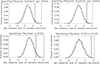 |
Fig. A.4. Mean detection level (calculated as in Figure 8) for void temperatures measured in norther galactic hemisphere only (upper left), southern galactic hemisphere only (upper right), lower redshift shell z < 0.02 only (lower left) and higher redshift shell 0.02 < z < 0.03 only (lower right). |
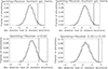 |
Fig. A.5. Maximum detection level (calculated as in Figure 8) for void temperatures measured in norther galactic hemisphere only (upper left), southern galactic hemisphere only (upper right), lower redshift shell z < 0.02 only (lower left) and higher redshift shell 0.02 < z < 0.03 only (lower right). |
The figure shows again the maximum and minimum detection levels taken over all choices of void radius fraction, void size sample and wavelet scale. We see a very similar detection level for the northern and southern hemispheres, in both cases about 2% of the simulations have larger detections. For the redshift shells, while both shells clearly show a strongly positive mean void temperature, the inner shell shows less detection than the outer shell, with about 5% simulations having larger detections in the inner shell and 0.3% in the outer shell. Note however that the volume of the inner shell z < 0.02 is much smaller than the outer shell 0.02 < z < 0.03. In order to further test consistency between redshift shells, we also split the observed volume inside z < 0.03 in two equal volume shells, z < 0.0238 and 0.0238 < z < 0.03. In Figure A.6 we show the results. Now the significance level is very similar for both redshift shells with about 1% simulations with higher detections in both shells. In summary, the results show a remarkable consistency between all these very different data splits.
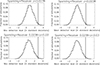 |
Fig. A.6. Same as Figure 8, but for the equal volume redshift split. Upper panels: Maximum (left) and mean (right) detection level using only voids in the most nearby shell z < 0.0238. Lower panels: Maximum (left) and mean (right) detection level using only voids in the second shell 0.0238 < z < 0.03. |
All Tables
Significances of void temperatures on wavelet-transformed SMICA maps (with quadrupole removed).
Significances of void temperatures on wavelet-transformed SMICA maps (with quadrupole removed) using only voids with negative density along the LOS, ΔLOS < 0.
Significances of SPARKLING void temperatures on wavelet-transformed SMICA maps (with quadrupole removed).
Significances of REVOLVER void temperatures on wavelet-transformed SMICA maps (with quadrupole removed).
Significances of SPARKLING void temperatures on wavelet-transformed SMICA maps (with quadrupole removed) using only voids with ΔLOS < 0.
All Figures
|
Fig. 1. Void weight maps. Left panels: Based on 200 void maps created from SPARKLING combining 100 realizations for the volume-limited sample of galaxies and 100 realizations from the sample using all galaxies. Right panels: Based on Revolver voids identified in the sample using all tracers as well as in the volume-limited sample. Each pixel represents a weight proportional to how many times that pixel was flagged as belonging to a void among those 200 void maps (SPARKLING) or among overlapping voids (REVOLVER). In these maps, a pixel was defined as belonging to a void when it was found within r < 0.5Rvoid for voids identified in the redshift range z = [0, 0.03] based on the 2MRS redshift catalogue. The upper panels show the result when all open voids were included, the middle panels for all voids larger than the median size of a given void set, and the lower panels for the largest quartile of voids. Similar void maps (not shown) were created using only pixels within r < 0.25Rvoid and r < 0.75Rvoid. |
| In the text | |
|
Fig. 2. Definition of ΔLOS considering the density within the solid angle subtended by the void between 1 and 3Rvoid. |
| In the text | |
|
Fig. 3. Combined weight maps created from the mean between the REVOLVER void maps and the SPARKLING void maps in Figure 1. The more times a pixel has been flagged as belonging to a void in SPARKLING and REVOLVER, the higher the pixel weight. A weight larger than 0.5 indicates that the pixel has been flagged as a void several times in both methods. From upper to lower panels, the void weight map based on: all open voids, the largest half of the voids, and the larger quartile of voids. |
| In the text | |
|
Fig. 4. Planck SMICA CMB temperature fluctuation map, masked such that only the areas around nearby galaxies (upper panel) and voids (lower panel) are clearly visible. The mask consists of holes of 1 Mpc radius around all large nearby spiral galaxies in the most massive galactic filaments within z < 0.02 (see H2025 for details). The void holes includes one realization of SPARKLING voids, including all voids with Δ23 < 0 out to z < 0.03 and extend to 1/2 void radius. The full CMB temperature map can be seen in the background. It can clearly be seen that the CMB temperature is mostly negative around galaxies and mostly positive in voids. |
| In the text | |
|
Fig. 5. Mean CMB temperature within 0.5Rvoid of each individual void for voids within the largest quartile. Voids are taken from the combined Sparkling sample, where only voids appearing in > 50% of the random realizations are included, corresponding to the voids that have the largest weights in the void weight maps of Figure 1. The fact that the void position and radius differ slightly for different realizations is reflected in the varying temperature within one single void for some of the voids. |
| In the text | |
|
Fig. 6. Mean CMB temperature in radial bins around voids: the black line shows the temperature taken from the largest quartile and the yellow line the one from all open nearby voids in the Planck SMICA CMB temperature fluctuation map with the quadrupole removed. Each bin is taken as 1/5 of the void radius. The grey bands show the 67%, 95%, and 99.7% confidence intervals based on 10 000 simulated maps for the largest quartile of voids and the dashed yellow line shows the corresponding 95% interval for the sample of all voids. Note that the profiles are only taken around voids with a central weight of > 0.5 in the void weight map (Figure 3), ensuring that the voids used for measuring the profile are flagged as a void in most random realizations of SPARKLING as well as in REVOLVER. |
| In the text | |
|
Fig. 7. Variance-weighted temperature difference between the mean CMB temperature in voids (inner temperature profile bin of the largest quartile of voids from Fig. 6) and the mean CMB temperature around galaxies (from H2025). The histogram shows the temperature difference in 10 000 SMICA simulations in terms of standard deviations calibrated on simulations. The red curve shows a Gaussian fit to the histogram. The blue line shows the corresponding difference in the data. |
| In the text | |
|
Fig. 8. Histograms showing the maximum detection level for void temperatures (upper left panel; 0.2% of the simulations have a higher maximum detection level), the mean detection level for void temperatures (upper right panel; 0.2% of the simulations have a higher mean detection level), the maximum detection level for void temperatures using only voids with ΔLOS < 0 (lower left panel; 0.03% of the simulations have a higher maximum detection level), and the mean detection level for void temperatures using only voids with ΔLOS < 0 (lower right panel; 0.09% of the simulations have a higher mean detection level). All cases are based on 9000 simulations and the free parameters (void size, wavelet scale, and the ratio of the void radius) are either varied to optimize the detection for each simulation (for maximum detection) or the significances are averaged over the parameter values in Table 1 (mean detection). The vertical lines show the same number for the real data. |
| In the text | |
|
Fig. 9. Mean (upper panel) and maximum (lower panel) detection levels in mocks (black histogram) and in 100 realizations of 2MRS voids. In the same way as in Fig. 8, we calculated the mean and maximum detection levels taken over the different parameter variations shown in Table 1 for the void sets of each individual mock catalogue and for 100 SPARKLING void realizations based on 2MRS data. All temperatures were calculated on the actual Planck SMICA CMB map and significances calibrated on the corresponding CMB simulations. |
| In the text | |
|
Fig. 10. Histogram showing the mean detection level for void temperatures over the free parameters (void size, wavelet scale, and ratio of void radius) for each of our 1000 simulations using only voids with ΔLOS < 0. The vertical line shows the same number for the real data. Results are shown for the Smica NO-SZ map where contamination from the SZ effect has been removed, the SEVEM cleaned frequency bands at 100GHz and 217GHz, the WMAP cleaned Q-band at 41Ghz, and the SEVEM cleaned map from the last PR4 Planck release. |
| In the text | |
|
Fig. 11. Void wavelet temperatures of voids with Rvoid within the largest quartile in 100 simulated CMB maps without (upper panel) and with (lower panel) the quadrupole removed. Black histograms show the void temperatures of the 100 simulations (of 10 000) with the coldest mean CMB temperature around galaxies and red histograms show the 100 simulations with the hottest temperature around galaxies. Blue line show the void temperature in Planck data. The histogram is shown with very small bins such that individual simulations are visible. |
| In the text | |
 |
Fig. A.1. Same as Figure 6 but only for SPARKLING voids. |
| In the text | |
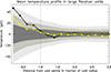 |
Fig. A.2. Same as Figure 6 but only for REVOLVER voids. |
| In the text | |
|
Fig. A.3. Same as Figure 8, but for SPARKLING and REVOLVER voids separately. Left column: max values, right column: mean values, upper row: SPARKLING open voids, middle row: SPARKLING voids with ΔLOS < 0, lower row:REVOLVER voids. |
| In the text | |
|
Fig. A.4. Mean detection level (calculated as in Figure 8) for void temperatures measured in norther galactic hemisphere only (upper left), southern galactic hemisphere only (upper right), lower redshift shell z < 0.02 only (lower left) and higher redshift shell 0.02 < z < 0.03 only (lower right). |
| In the text | |
|
Fig. A.5. Maximum detection level (calculated as in Figure 8) for void temperatures measured in norther galactic hemisphere only (upper left), southern galactic hemisphere only (upper right), lower redshift shell z < 0.02 only (lower left) and higher redshift shell 0.02 < z < 0.03 only (lower right). |
| In the text | |
|
Fig. A.6. Same as Figure 8, but for the equal volume redshift split. Upper panels: Maximum (left) and mean (right) detection level using only voids in the most nearby shell z < 0.0238. Lower panels: Maximum (left) and mean (right) detection level using only voids in the second shell 0.0238 < z < 0.03. |
| In the text | |
Current usage metrics show cumulative count of Article Views (full-text article views including HTML views, PDF and ePub downloads, according to the available data) and Abstracts Views on Vision4Press platform.
Data correspond to usage on the plateform after 2015. The current usage metrics is available 48-96 hours after online publication and is updated daily on week days.
Initial download of the metrics may take a while.