


| Issue |
A&A
Volume 710, June 2026
|
|
|---|---|---|
| Article Number | A408 | |
| Number of page(s) | 12 | |
| Section | Extragalactic astronomy | |
| DOI | https://doi.org/10.1051/0004-6361/202659563 | |
| Published online | 01 July 2026 | |
XRISM/Resolve probes a possible “raining” absorber in Mrk 509
1
INAF – Osservatorio di Astrofisica e Scienza dello Spazio di Bologna, Via Gobetti 101, I-40129 Bologna, Italy
2
INAF – Osservatorio Astronomico di Brera, Via Bianchi 46, I-23807 Merate (LC), Italy
3
INAF – Osservatorio Astronomico di Roma, Via Frascati 33, I-00078 Monte Porzio Catone, Italy
4
INAF – Istituto di Astrofisica e Planetologia Spaziali, via Fosso del Cavaliere 100, I-00133 Roma, Italy
5
Institut de Recherche en Astrophysique et Planétologie, 9 avenue du Colonel Roche, Toulouse 31028, France
6
INAF – Osservatorio Astrofisco di Arcetri, largo E. Fermi 5, 50127 Firenze, Italy
7
Dipartimento di Matematica e Fisica, Università degli Studi Roma Tre, Via della Vasca Navale 84, I-00146 Roma, Italy
8
Department of Physics and Astronomy, College of Charleston, Charleston, SC 29424, USA
9
SRON Netherlands Institute for Space Research, Leiden, The Netherlands
10
Leiden Observatory, University of Leiden, P.O. Box 9513, NL-2300 RA, Leiden, The Netherlands
11
Cahill Center for Astronomy & Astrophysics, California Institute of Technology, 1216 East California Boulevard, Pasadena, CA 91125, USA
12
Quasar Science Resources SL for ESA, European Space Astronomy Centre (ESAC), Science Operations Department, 28692 Villanueva de la Cañada, Madrid, Spain
13
Space Science Data Center, Agenzia Spaziale Italiana, Via del Politecnico snc, 00133 Roma, Italy
14
Université Grenoble Alpes, CNRS, IPAG, 38000 Grenoble, France
15
INAF–IASF Palermo, Via U. La Malfa 153, I-90146 Palermo, Italy
16
Instituto de Estudios Astrofísicos, Facultad de Ingeniería y Ciencias, Universidad Diego Portales, Av. Ejército Libertador 441 Santiago, Chile
17
Dipartimento di Fisica e Astronomia ‘Augusto Righi’, Università degli Studi di Bologna, Via Gobetti 93/2, I-40129 Bologna, Italy
★ Corresponding author: This email address is being protected from spambots. You need JavaScript enabled to view it.
Received:
23
February
2026
Accepted:
4
May
2026
Abstract
Context. X-ray spectroscopy of active galactic nuclei (AGNs) offers unique insights into the reprocessing of radiation and the gas dynamics near supermassive black holes. The Seyfert 1 galaxy Mrk 509 is an ideal laboratory for these studies. It is in fact known for its complex iron K emission and one of the four or five AGNs to date in which evidence of transient, blue- and redshifted absorption features indicative of high-velocity flows has been detected in X-rays.
Aims. We present the first high-resolution 2–10 keV spectrum of Mrk 509 obtained with the XRISM/Resolve calorimeter. Our primary goals are to disentangle the narrow and broad emission features and to place stringent constraints on the kinematics and physical locations of circumnuclear gas flows, specifically searching for signatures of accretion and feedback.
Methods. We analyzed 106 ks of XRISM/Resolve data, complemented by simultaneous XMM-Newton and NuSTAR observations, which we used to constrain the broadband continuum. We modeled the spectra using self-consistent reflection models for the continuum and the emission lines, and employed photoionized plasma models to characterize discrete, ionized absorption features.
Results. The XRISM/Resolve spectrum reveals a narrow Fe Kα core resolved with σ ≃ 10 eV (vFWHM∼ 1100 km/s). The best-fit model includes a broader component with σ ∼ 450 eV. We also find tentative evidence of discrete absorption features at rest-frame energies of E ∼ 6.2 keV. When modeled as an ionized absorber (with a significance of ∼3.6σ), the data suggest the gas is redshifted relative to the systemic velocity, corresponding to an inflow of material with vin ∼ 11 000 km s−1, located within the inner few thousand gravitational radii.
Conclusions. The narrow Fe Kα emission is consistent with an origin in the dusty torus, while the broad component arises from broad-line-region scales or the accretion disk (R ∼ 30–120 rg). This scenario is strongly corroborated by our relativistic reflection modeling, which restricts the inner edge of the emitting region to distances greater than 27 rg. If confirmed by future observations, the high-velocity inflow would likely represent dense, fragmented clumps of a “failed wind” raining back onto the accretion disk, providing potential direct evidence that nonstandard accretion processes may coexist with canonical disk-like flows in the inner regions of AGNs.
Key words: galaxies: active / galaxies: individual: Mrk509 / galaxies: Seyfert / X-rays: galaxies
© The Authors 2026
 Open Access article, published by EDP Sciences, under the terms of the Creative Commons Attribution License (https://creativecommons.org/licenses/by/4.0), which permits unrestricted use, distribution, and reproduction in any medium, provided the original work is properly cited.
This article is published in open access under the Subscribe to Open model. This email address is being protected from spambots. You need JavaScript enabled to view it. to support open access publication.
1. Introduction
X-ray spectroscopy of active galactic nuclei (AGNs) provides an unparalleled tool for probing the extreme environments surrounding supermassive black holes (SMBHs), which are believed to coevolve with their host galaxies (e.g., Kormendy & Ho 2013; Heckman & Best 2014). Among the features observed, the iron Kα (Fe Kα) emission line at 6.4 keV is nearly ubiquitous and serves as a powerful tracer of circumnuclear gas (Nandra et al. 2007). The line’s profile is a key diagnostic of its physical origin: a narrow core is typically associated with reflection from distant material, such as the molecular torus (see Antonucci 1993), while a broad and relativistically skewed profile is the hallmark of emission from the inner accretion disk, just a few gravitational radii ( , where G is the gravitational constant, M is the mass of the SMBH, and c is the speed of light) from the SMBH (e.g., Tanaka et al. 1995; Fabian et al. 2000).
In addition to emission, AGN spectra often exhibit absorption features from ionized gas along the line of sight. Blueshifted absorption lines are clear signatures of outflows, with the most extreme examples being the ultrafast outflows (UFOs) that reach velocities up to v∼ 0.1−0.5c (e.g., Chartas et al. 2002, 2021; Pounds et al. 2003; Reeves et al. 2002, 2009, 2014, 2018; Dadina et al. 2005, 2018; Cappi 2006; Cappi et al. 2009; Tombesi et al. 2010, 2011, 2013; Gofford et al. 2013; Nardini et al. 2015; Matzeu et al. 2016, 2017, 2023; Braito et al. 2018; Gianolli et al. 2024; Xrism Collaboration 2025a). These powerful winds are considered a key channel for AGN feedback, regulating SMBH growth and star formation (e.g., King & Pounds 2015; Gaspari et al. 2020; Laha et al. 2021). Conversely, redshifted absorption features, indicative of infalling material, remain far rarer. Only a small number of candidate ultrafast inflows (UFIs) exist in the literature (e.g., Nandra et al. 1999; Dadina et al. 2005; Yaqoob & Serlemitsos 2005; Longinotti et al. 2007; Giustini et al. 2017; Peca et al. 2025). Ultrafast inflows offer a unique window into nonstandard accretion processes, such as fallback from “aborted jets” or “failed winds”, where the launched material fails to escape the SMBH’s gravitational pull (e.g., Ghisellini et al. 2004; Proga & Kallman 2004; Giustini & Proga 2019).
The bright, nearby Seyfert 1 galaxy Mrk 509 (z = 0.034, Huchra et al. 1993) is an ideal laboratory for studying these phenomena. Extensive monitoring has revealed a complex Fe Kα structure composed of a constant narrow core and a variable, resolved component (Ponti et al. 2013). Reverberation mapping has shown that the resolved component responds to continuum variations on timescales of days, placing its origin within a few light-days from the central engine (Ponti et al. 2013). Furthermore, Mrk 509 is one of the very few objects where transient, redshifted Fe K absorption lines–the potential signature of a UFI–have been reported in the literature (Dadina et al. 2005). The source has also shown evidence of variable, highly ionized outflows with velocities up to ∼14 000 km s−1 (Dadina et al. 2005; Ponti et al. 2009; Cappi et al. 2009; Tombesi et al. 2010).
In this work, we present the first high-resolution X-ray spectrum of Mrk 509 (MBH ∼ 1.02 × 10⁸ M⊙, Li et al. 2024) in the 2–10 keV band, obtained with the Resolve (Ishisaki et al. 2025) instrument on board the X-Ray Imaging and Spectroscopy Mission (XRISM, Tashiro et al. 2024). Leveraging the unprecedented spectral resolution of Resolve (≈4.7 eV at 6 keV, Ishisaki et al. 2025), our analysis aims to disentangle the complex emission and absorption features in the Fe K band. This will allow us to place new, stringent constraints on the physical properties, dynamics, and location of the different gas flows, from the reverberating reflector to the transient inflows and outflows.
The approved XRISM observation of Mrk 509 (P.I. M. Cappi) was designed with three primary scientific goals: i) confirming and studying gas in- and outflows, ii) defining the origin of the neutral Fe Kα line, and iii) understanding the origin of the ionized iron complex. The XRISM proposal triggered the organization of a broader, complementary multiwavelength campaign with the NuSTAR, XMM-Newton, Swift, and optical telescopes (NTT/TNG) to provide a complete view of the source. However, in this work, we focus mainly on the results obtained analyzing the XRISM/Resolve data and taking advantage of the XMM-Newton (Jansen et al. 2001) and NuSTAR (Harrison et al. 2013) capabilities to define the baseline X-ray continuum of Mrk 509. The broadband properties of the source, including the spectral complexities in the soft energy band and the source variability, will be addressed in an upcoming paper (Missaglia et al., in prep.).
2. Data reduction and analysis
XRISM observed Mrk 509 on November 11, 2024. The high-resolution Resolve calorimeter operated in its standard PX NORMAL mode. We were unable to use the Xtend data due to a camera anomaly during this observation. While prior studies with missions such as XMM-Newton and Chandra have characterized Mrk 509 at CCD resolutions, this work focuses primarily on the new, high-resolution Resolve spectrum. Nonetheless, we also present an analysis of the NuSTAR and XMM-Newton data collected via DDT observations triggered to coordinate with the XRISM/Resolve pointing. These data are particularly important for properly constraining the continuum emission in the 2–10 keV band. The source was observed twice with NuSTAR in November 2024 for a total exposure of ∼34 ks. Quasi-simultaneous observations (three in total) were also performed with XMM-Newton. Table 1 lists the details of all observations, while Fig. 1 displays the temporal coverage of each pointing.
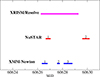 |
Fig. 1. Time scheme of the X-ray observation presented in this work. The horizontal lines represent the total observation times. |
The XRISM/Resolve data were reduced using the XRISM Quick-Start Guide v2.3, HEASOFT version 6.34, and the associated calibration files. Briefly, the data were filtered to exclude anomalies in low-Earth orbit as well as events from the calibration pixel (pixel 12) and pixel 27 with abnormal gain behavior. The data were further screened to include only high-resolution primary (Hp) events. The technical report from the instrument team confirms the nominal functioning of the Resolve instrument during the observation, with an energy resolution of ∼4.6 eV at the Fe55 reference energy, and no gain shift was detected over the course of the exposure. A light curve of the event list reveals flux variability, with distinct brightening during the final third of the observation (see Fig. 2). A search for spectral variability, performed by analyzing the ratio between the 2–5 keV and 5–12 keV bands, indicates no strong spectral variability associated with this change in flux (see Fig. 2). For this reason, a time-averaged spectral analysis is well justified. The resulting spectrum was built with default bins of 0.5 eV, and the tools rslmkrmf and xaarfgen were used to make the redistribution matrix file (rmf) and ancillary response file (arf). We elected to create a “Large” (Gaussian core plus exponential tail and Si Kα instrumental line plus escape peak) rmf. After screening (e.g., pixel-pixel coincident events), the net Resolve exposure time was approximately 106 ks. Finally, following standard procedure (see, for example, Xrism Collaboration 2025a), we treated the background by directly incorporating the generated non-X-ray background (NXB) into our spectral models.
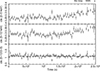 |
Fig. 2. Non-background-subtracted XRISM/Resolve light curves of Mrk 509 shown in the 2–5 keV (top panel) and 5–12 keV (middle panel) energy bands. Bottom: Corresponding hardness ratio. A clear brightening trend is evident toward the end of the observation, but it is not accompanied by significant spectral variability. |
We processed XMM-Newton EPIC-pn data using the Science Analysis System (SAS) v21.0. Calibrated event lists were generated from the raw observation data files (ODFs) using the standard pipeline chains. The camera was operated in small window mode to minimize photon pileup. The resulting event lists were filtered to remove periods of high particle background flaring, and standard pattern selection criteria were applied. For the spectral analysis, source counts were extracted from a 28″-radius circular region centered on the source’s position. The background spectrum was estimated from two nearby, source-free 26″-radius circular regions located on the same CCD. The corresponding arfs and rmfs were generated for spectral fitting.
Similarly, we processed NuSTAR data for both observations using the NuSTAR Data Analysis Software (NuSTARDAS) package. Source spectra were extracted from a 1.5′-radius circular region centered on the target. For the background, we used a separate 1.88′-radius circular region located on the same detector, chosen to be free of source contamination. The nuproducts task was used to filter the data, apply standard screening criteria, and generate all final data products, including spectra and response files.
To prepare the data for spectral fitting, we applied specific grouping and band-pass selections for each instrument. The XRISM/Resolve data were analyzed in the 2–12 keV band to avoid calibration uncertainties at the spectral boundaries. Following Mizumoto et al. (2026), these data were uniformly grouped by a factor of 10, resulting in a final bin size of 5 eV (Tashiro et al. 2025). Although this slightly overbins the nominal energy resolution of Resolve, we adopted this conservative approach to enhance the signal-to-noise ratio (S/N) per spectral bin, facilitating both the detection and the modeling of weak and broad spectral features. Furthermore, the choice of a constant energy binning was dictated by the mathematical requirements of certain convolution models used in our analysis, such as gsmooth (see Sect. 4). Finally, we anticipate here that this choice does not strongly impact our data analysis, since the width of the narrow Fe emission line is found to be on the order of σ∼10 eV (see Sect. 4). The EPIC-pn data were grouped to a minimum of 100 counts per bin, while the NuSTAR data were similarly grouped to ensure a minimum of 50 counts per bin.
3. Defining a baseline model using the 2–60 keV XMM-Newton and NuSTAR data
A simple power-law model to simultaneously fit the 2–60 keV XRISM/Resolve, the XMM-Newton/EPIC-pn, and NuSTAR data reveals several key features (see Fig. 3, upper panel). The most prominent are: a) a narrow emission line centered at E ≈ 6.4 keV and b) a broad excess spanning the 4–7 keV band.
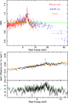 |
Fig. 3. Upper panel: 2–60 keV ratio between the data and a simple power-law model for the Mrk 509 X-ray data taken during this campaign (see Table 1), expressed in units of standard deviations. Here, for clarity purposes, the data have been strongly rebinned (each data point has a 25σ significance). Lower panel: 2–12 keV spectrum of Mrk 509 observed by XRISM/Resolve. The orange line represents the best fit using a simple power-law model. In this case, the Resolve data have also been rebinned (each data point here has a significance of 15σ) for visual clarity. |
To determine the best modeling of the continuum, we analyzed the 2–60 keV data from XMM-Newton/EPIC-pn and NuSTAR only. At this stage, we excluded the data below 2 keV to avoid the complexities associated with the known strong soft excess (see e.g., Mehdipour et al. 2011; Petrucci et al. 2013, 2018) and the complex warm absorber (Kaastra et al. 2012) that strongly affect the low energy (E ≤ 2 keV) spectrum of Mrk 509.
The spectral analysis, including all NuSTAR and EPIC-pn datasets collected during our campaign (total of five observations; see Table 1), was performed using the XSPEC fitting package v12.15.1 (Arnaud et al. 1999). We included a cross-normalization constant to account for differences in absolute calibration between the instruments, as well as for intrinsic source variability (see columns X-XIII in Table 2). Mrk 509 is known to exhibit X-ray flux variations on typical timescales of days (Kumari et al. 2021). This behavior is indeed confirmed by the XRISM/Resolve light curves (see Fig. 2).
Observation log with net exposure times.
We started using a simple cutoff power-law model plus a Gaussian emission line to reproduce the Fe Kα feature. The high-energy cutoff was fixed at a fiducial value of Ec = 150 keV (see Petrucci et al. 2013), as the current data do not provide meaningful constraints on this parameter. We fixed the line width to σ = 20 eV, consistent with the narrow feature clearly resolved in the XRISM/Resolve data (see both panels of Fig. 3).
The energy of the Gaussian is found to be consistent with neutral iron (E = 6.39 ± 0.02). If we model the remaining curvature observed in the 4–7 keV band with a broad Gaussian, we find that its centroid is at E ∼ 5.4 keV with a width of σ ∼ 1.5 keV. This hence indicates that the underlying continuum may be poorly described by simple power-law modeling. We also fixed the broad Gaussian to the same energy of the narrow component; however, residuals remain.
To describe the residual spectral curvature observed at 4–7 keV, we explored different scenarios using different continuum models. These include i) a neutral, partial absorber (models PC1 and PC2 in Table 2) and/or ii) a relativistic scenario due to reflection from material in the disk (models RR1-RR2 with relxill in Table 2).
Best-fits of the XMM-Newton EPIC-pn plus NuSTAR data.
The partial covering models provide a robust description of the broadband data. Specifically, when a simple Gaussian line is added, the feature is found to be consistent with emission from cold material (see the PC1 model in Table 2). Furthermore, motivated by the XRISM/Resolve spectra (see Sect. 4)–which clearly reveal a narrow core–we tested a scenario where this component originates from neutral reflection from distant material (modeled using pexmon, Nandra et al. 2007). This approach significantly improves the quality of the fit (see model PC2 in Table 2). Finally, we tested for an additional broad Fe Kα Gaussian component but found it statistically unnecessary when adopting the partial covering model. This modeling, moreover, allows us to recover photon index values (Γ ∼ 1.7) in agreement with those previously reported in literature (Γ ∼ 1.6–1.7; Pounds et al. 2001; Ponti et al. 2009, 2013) and with the average value found in AGN samples (Nandra & Pounds 1994; Piconcelli et al. 2005; Dadina 2007, 2008; Bianchi et al. 2009; Ricci et al. 2017; Middei et al. 2019).
To test the relativistic reflection scenario, we initially applied a model consisting of a relativistic reflection component (relxill, Dauser et al. 2014) and a narrow Fe Kα Gaussian emission line. As in the previous case, we fixed the high-energy cutoff to Ec = 150 keV and, as shown in Petrucci et al. (2013), we fixed the inclination angle of the system at Θ = 30°. This baseline model provides a poor description of the data (model RR1 in Table 2), leaving significant positive residuals. Similarly to the simple power-law model, the inclusion of a partial covering component is also required (model RR2 in Table 2). This addition significantly improves the fit (see residuals in the lower panel of Fig. 4). Left free to vary, the black hole spin (indicated by the a parameter in Table 2) remains unconstrained, while the reflection component is consistent with that measured in the PC2 model. Following the approach adopted for model PC2, we also tested a scenario where the narrow Fe Kα line originates from the distant torus (modeled using pexmon). This resulted in a significantly poorer fit to the data than model RR2. Finally, it is worth noting that in all these relativistic scenarios, the recovered photon index of the primary emission is consistently flat (see Table 2).
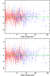 |
Fig. 4. Upper panel: Residuals of the PC2 model (neutral partial covering with distant reflection component). Lower panel: Residuals of the RR2 model (neutral partial covering with a relativistic reflection component and narrow Fe Kα Gaussian emission line). In all panels, the XMM-Newton data are in red, while the NuSTAR data are in blue. |
As reported in Table 2, the PC2 and RR2 models provide the best fits to the broadband data (see also the two panels in Fig. 5 for a zoom-in on the residuals in the Fe K band for the PC2 and RR2 best fits). The RR2 scenario introduces four additional free parameters but provides only marginal statistical improvement (ΔC = 10) and, crucially, the PC2 model yields a primary photon index in perfect agreement with values typically observed in Seyfert galaxies (Nandra & Pounds 1994; Ricci et al. 2017). In the latter scenario, we assume that the reflection component originates in the torus, as suggested by the narrowness of the Fe K features (see also Section 4). Consequently, in our model, this component is not affected by the partial absorber, which is assumed to cover only the emission originating in the Mrk 509 core.
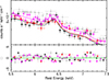 |
Fig. 5. Zoom-in on the 5.5–7.5 keV range PC2 model (see Table 2). XMM-Newton data observation 1 is in black, observation 2 is in red, and observation 3 is in magenta. The NuSTAR data are in gray. There are no significant residuals. |
4. The XRISM/Resolve view of the Fe complex
Building on the results presented above, we tested both the simple partial covering model (named PC in the following) and the relativistic scenario (named RR in the following) on our XRISM/Resolve data. Starting with the PC2 scenario, we used a simple zpcfabs model (see Sect. 3), yielding a canonical photon index of Γ ∼ 1.8, in excellent agreement with the values obtained from XMM-Newton EPIC-pn and NuSTAR data. In this scenario, the primary emission is partially absorbed (covering fraction Cf ∼ 0.3) by a neutral component with a column density of NH ∼ 1.3 × 1023 cm−2 (again consistent with the broadband fit obtained, as discussed in Sect. 3).
The narrow Fe Kα line was modeled using the zFeklor model (this model includes seven Lorentzian profiles to describe the line; see Hölzer et al. 1997). The energy centroid of this model is not a free parameter in the fit. When its redshift is allowed to vary, the best fit is obtained at  (errors correspond to the 90% confidence level here and throughout the paper, unless stated otherwise), which is in good agreement with the redshift of the source. To estimate the line width, we applied a gsmooth convolution model to the zFeklor component, yielding σn = 10 ± 5 eV and an equivalent width of EWn ∼ 27 eV. These parameters strongly suggest that this feature originates far from the central SMBH.
Some residuals remain at the rest energy of the Fe Kα complex, between 6.5 and 6.7 keV (see Fig. 6). Following previous results on Mrk 509 (Ponti et al. 2009, 2013; Yaqoob et al. 2003; Yaqoob & Padmanabhan 2004) and the features observed in NGC 4151 (XRISM Collaboration 2024), we added a broad Gaussian component that improves the fit (ΔC ∼ 20 for three parameters of interest). The line parameters are Eb ≃ 6.49 ± 0.15 keV, a width of σb ≃ 320 ± 220 eV, and EWb ≃ 90 ± 50 eV. The width of this feature (v ∼ 14 800 km/s) suggests an origin close to the SMBH, corresponding to r ∼ 50 rg.
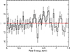 |
Fig. 6. 5–7.5 keV zoom-in on the Resolve residuals for the model including cold partial covering and the zFeKlor component to account for the narrow Fe Kα complex. The data are strongly rebinned for clarity purposes (each data point in the plot has a 20σ significance). The most significant deviations from the model are a possible absorption feature at E ∼ 6.2 keV and a broader component in the 6–6.8 keV range. |
Interestingly, very similar results are obtained in the RR scenario (see the RR-I model in the lower panel of Table 3). Assuming a maximally spinning SMBH and a standard radial emissivity profile (ϵ ∝ r−3), we derive a lower limit for the inner edge of the reflection disk of rin ≥ 27 rg (consistent with that obtained with the broad Gaussian), along with a low reflection fraction of R ∼ 0.17 and a consistent broadening of the narrow FeK line.
Partial covering models.
4.1. Characteristics of the distant reflection
As shown in Table 3, the properties of the narrow emission line are consistent with an origin far from the SMBH in both the PC and the RR scenarios. To achieve a more robust physical characterization, we used the MYTorus model (Murphy & Yaqoob 2009; Yaqoob 2012) to account for this component in the PC scenario. MYTorus was in fact specifically designed for modeling the X-ray spectra of AGNs and their associated fluorescent lines originating in the dusty torus. Specifically, we added the MYTorusL (Fe Kα and Fe Kβ fluorescent emission lines, latest available version) and MYTorusS (reflected continuum) components to the primary power-law continuum. We linked their column densities to ensure self-consistency and fixed the inclination angle at Θ = 0°, thereby assuming the matter lies out of the line of sight. Not only does MYTorusL reproduce the narrow Fe line profile (similar to zFeklor), but it also crucially ensures proper treatment of the Compton shoulder. The photon index of the MYTorus components was tied to that of the primary power law to maintain a uniform spectral slope. Since a preliminary Gaussian fit showed the narrow Fe line energy to be consistent with 6.4 keV, we fixed the redshift of the MYTorus components to that of Mrk 509, assuming no additional bulk motion. Finally, to test for line broadening, we applied a Gaussian smoothing kernel (gsmooth in XSPEC) to the MYTorusL component.
As shown in Fig. 7, the material responsible for the narrow emission lines (Fe Kα and Fe Kβ) must be located far from the SMBH, given that the line broadening is on the order of σ = 10 ± 5 eV. This corresponds to a velocity of v ∼ 1000 ± 500 km s−1 (FWHM), a result that is well in agreement with that obtained using the zFeklor models and implying a distance on parsec scales for a SMBH with a mass of M ∼ 108 M⊙ (Peterson et al. 2004; Li et al. 2024). This result strongly supports the hypothesis that the Fe K lines originate in the torus (Antonucci 1993).
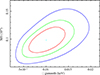 |
Fig. 7. Confidence contours between the column density and broadening kernel for the distant reflector from MYTorus modeling of the reflector and associated lines (see Sect. 4.1). |
On the other hand, the column density of this component is relatively lower (NH ∼ 1023 cm−2) than the average value (NH ∼ 1024 cm−2) found in samples of Compton-thin AGNs using NuSTAR. However, they are in good agreement with the lower end of the column densities measured for the Compton-thin sources in the sample (Zhao et al. 2021). It is worth noting here that adding MYTorus in the RR scenario does not meaningfully improve the fit.
4.2. An infalling partial absorber
As described in the previous sections, a partial absorber of the primary emission is able to model the data well in both the PC and RR scenarios. As shown in Fig. 8 (PC scenario), some spectral features remain visible in the spectrum of Mrk 509, a trend also observed in the RR case. In particular, possible absorption features can be identified at E ∼ 4.2, 6, 7 and, possibly, at 8–9 keV. When all these features are modeled with a Gaussian absorption line of fixed width (σ = 5 eV), the statistically strongest line is detected at  keV (see Fig. 9 for the PC case). This addition improves the fit by ΔC ∼ 13 in both scenarios.
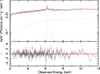 |
Fig. 8. 2–12 keV spectrum of Mrk 509 modeled with partial covering of the primary emission, broad Gaussian line, and neutral reflection (MYTorus model; see model I in Table 3). The components are shown as dotted lines: absorbed power-law (red), absorbed broad Gaussian line (blue), MYTorusL (magenta), and MYTorusS (orange). |
To assess the importance of this absorption feature, we employed the small sample Akaike information criterion (AIC, Akaike 1974). Specifically, we computed the change in AIC (ΔAIC) when the line is removed from the model. A ΔAIC below −2 provides strong evidence that the feature is required, while a value below −10 would indicate it is essential for explaining the data. In our case, ΔAIC ∼ − 9 suggests the presence of this absorption line. Furthermore, a closer inspection of the ∼6 keV region suggests a more complex structure, with possible multiple dips between the 6.0 and 6.1 keV rest frame (see the lower panel of Fig. 9).
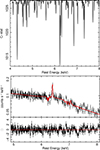 |
Fig. 9. Upper panel: Confidence contours (rest-frame energies) from the blind search for possible absorption features (see Sect. 4.2). Lower panel: Zoom-in on the spectral range where the strongest feature (absorption line at |

Given the apparent complexity of the absorption feature, we used photoionized absorber models as a partial covering component to fit the absorption feature at ∼6 keV. We created grid tables using the XSTAR code (Kallman & Bautista 2001) with an ionizing luminosity of L1 − 1000 Ry ≈ 3.1 × 1045 erg s−1 (see Sect. 4) and, following Petrucci et al. (2018), a SED dominated by a warm- plus hot-corona component tuned to the XMM-Newton and NuSTAR data (Missaglia et al. in prep.).
As a first step, we focused on the PC case and assumed a density of n = 108 cm−3 for the intervening gas, consistent with the absorber located at sub-parsec scales, comparable to the BLR. This is, for instance, supported by the unified stratification models of AGN winds (e.g., Tombesi et al. 2013; Gofford et al. 2013; Reeves et al. 2018; Serafinelli et al. 2019) and density diagnostics using metastable lines in similar Seyfert galaxies that typically yield n ≥ 108 cm−3 for the high-ionization phases (e.g., Mao et al. 2017). Moreover, following the estimate obtained in Sect. 4 for the PC case, we also tested a density of n ∼ 1010 cm−3, assuming that the matter emitting the broad Fe line is somehow linked to the material causing the partial absorption. In both scenarios, we fixed the matter turbulence to vturb = 100 km s−1 since the feature seems narrow (see Fig. 9). Models n8 and n10 and RR-n8 in Table 3 report the results obtained using these XSTAR grids. These models significantly improved the quality of the fit in both scenarios and provided a best-fit result with an absorbing gas density of n = 108 cm−3 and log ξ ∼ 2.5 (see models n8 and RR-n8 in Table 3 and Fig. 10).
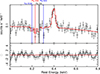 |
Fig. 10. 6.0–6.8 keV zoom-in on the spectral range where the strongest features from ionized gas are measured (model n8 in Table 3). The features measured in the 6.1–6.4 keV range are due to the Fe XVIII–Fe XXI lines. |
As a consistency check, we also tested a different photoionized model, namely the PHASE model, based on CLOUDY (Ferland et al. 1998). This model is designed to reproduce absorption features from an ionized plasma, where the central source emits an ionizing continuum with gas clouds intercepting the line of sight (model Ph in the upper part of Table 3). Although it provides poorer statistical fit to the data compared to the XSTAR grid, the PHASE model yields consistent properties for the absorbing gas.
Interestingly, by anchoring the models to the absorption features observed between ∼6–7 keV (see Fig. 11), all the above models imply that the matter causing the ionized absorption is measured at a redshift of zobs ∼ 0.074 (see the lower panel of Fig. 11). Since this finding is higher than the systemic redshift of Mrk 509 (zsou = 0.034 ± 0.001), it could–if confirmed–indicate that the absorbing matter is infalling toward the central SMBH. In this energy range, the lines are primarily due to Fe XVIII–Fe XXI transitions.
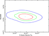 |
Fig. 11. Upper panel: 99%, 90%, and 68% confidence contours for the z vs. NH parameters obtained using model n8 in Table 3. |
To further test the significance of the infalling scenario, we performed Monte Carlo simulations under the PC scenario. Starting from the partial covering model (model I) presented in Table 3, we performed a suite of 1500 simulations of XRISM/Resolve spectra. These simulations were conducted using the rmf and arf generated for the data analysis, as previously described. To maintain consistency with the observational constraints, each simulated dataset was assigned an exposure time identical to that of the original observation. Subsequently, each of the 1500 simulated spectra was fitted using both the baseline Model I and the alternative model n8. For the model n8 fits, the ionization parameter was allowed to vary within the log(ξ/erg cm s−1) = 1.5–4.0 range, while the observed redshift was free to fluctuate between z = −0.2 and z = 0.2. To ensure that each single fit did not stack in local minima, we forced the procedure to search for the errors on all free parameters multiple times before and after running the steppar command on the ionization parameter, the redshift, the column density of the ionized absorber, and the continuum-free parameters. For every simulated dataset, we recorded the value of the C-statistic for both models to calculate the difference, Δ(C), which provides the statistical basis for our cumulative distribution analysis presented in Fig. 12. According to this test, our results have a significance of ∼3.6σ.
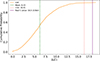 |
Fig. 12. Cumulative distribution of the ΔC statistic derived from 1500 Monte Carlo simulations, assuming Model I (see Table 2) as the null hypothesis. Synthetic XRISM/Resolve spectra were generated matching the exposure time of the real observation. For each simulation, ΔC is defined as the difference in the C-statistic between the best fits obtained modeling the simulated datasets with Model I and Model n8 in Table 2. The vertical green line indicates the mean simulated ΔC, while the red line marks the 3σ confidence threshold. The purple line represents the ΔC value observed in the real data. |
The current model produces residuals at a rest-frame energy of E ∼ 7.3 keV (see Fig. 9). Adding a simple Gaussian absorption line yields a marginal improvement to the fit (ΔC ∼ 14 for three additional free parameters). Nevertheless, the centroid energy of this feature (E ∼ 7.31 keV, σ ∼ 40 eV, and EW∼ 14 eV) is perfectly consistent with previous findings (Ponti et al. 2009). If identified with highly ionized iron such as Fe XXVI this absorption feature would indicate an outflowing wind with a velocity on the order of 13 500 km/s.
It is interesting to note that the partial absorber characteristics yield completely consistent results when using the RR baseline model instead of the PC scenario. As reported in the lower part of Table 3, utilizing an ionized rather than cold absorber significantly improves the fit (ΔC = 15 for two additional free parameters). More importantly, we obtain exactly the same properties for the absorber in terms of both its ionization state and velocity.
Finally, we tested the two scenarios by incorporating the NuSTAR data for observation 1 (performed within the Resolve pointing; see Fig. 1) and for observations 1 and 2 in the 10–60 keV range. From a statistical point of view, the two models perform identically, and the resulting parameters are fully consistent with those obtained using the Resolve data alone. The only notable difference lies in the cross-calibration constant between XRISM/Resolve and NuSTAR. In the PC case, we obtain a cross-calibration constant of cr = 1.08 ± 0.05, which is well in agreement with previous findings (Xrism Collaboration 2025b). Conversely, in the RR case, we measure a higher constant of cr = 1.21 ± 0.10
5. Discussion
The XRISM/Resolve spectrum of Mrk 509 displays the signatures of a complex structure at Fe K line energies. In particular, we detected:
-
a narrow Fe Kα component, most likely arising from the putative torus;
-
a relativistic or broad Fe Kα emission line originating from a region close to the central SMBH;
-
spectral features consistent with a partial absorber, potentially associated with an infalling flow, although this interpretation remains model-dependent.
We estimate the dust sublimation radius for Mrk 509 to be Rsub ≈ 0.74 pc, using the scaling relation in Barvainis (1987) for graphite grains with a sublimation temperature of Tsub ≈ 1500 K and a bolometric luminosity of Lbol ≈ 3.2 × 1045 erg s−1 (Kaastra et al. 2012; Detmers et al. 2011). In comparison, the measured width of the narrow Fe Kα core (σE ≈ 10 eV) corresponds to a virial emission radius of RFeK ≈ 2.0 pc, assuming a black hole mass of MBH ∼ 1.02 × 10⁸ M⊙ (Li et al. 2024). This places the bulk of the neutral iron emission outside the sublimation boundary (RFeK ∼ 2.7Rsub), indicating that the fluorescent reflector is located within the body of the dusty torus rather than at its innermost wall. This geometry is consistent with clumpy torus scenarios where X-ray fluorescence arises from cold, dusty clouds that are sufficiently shielded from the central engine (Ramos Almeida & Ricci 2017).
As presented in Sect. 4, the best modeling of the data is obtained using a broad Fe emission detected at E ≈ 6.5 ± 0.15 keV, with a width of σ ≈ 450 ± 150 eV, which implies a velocity dispersion of σv ≈ 21 000 km s−1. Adopting the virial assumption and the same black hole mass, we estimate an emission radius of Rbroad ≈ 0.001 pc (∼30–120 rg). This places the production region roughly three orders of magnitude closer to the central engine than the dusty torus, consistent with the typical spatial scales of the BLR and the outer accretion disk. These spectral parameters are statistically consistent with those reported in Ponti et al. (2013) based on long XMM-Newton observations (E = 6.43 ± 0.01 keV and σ = 0.22 ± 0.05 keV). Notably, this physical scale is perfectly corroborated by the scenario in which the broad line originates from the relativistic reflection of the accretion disk; when explicitly modeled as disk reflection, we derive a lower limit of r ≥ 27 rg for the inner emission radius in excellent agreement with the virial estimate.
Our results for Mrk 509 align remarkably well with the emerging picture of the central engine revealed by recent XRISM observations of other Type 1 AGNs. In NGC 4151, the XRISM Collaboration (XRISM Collaboration 2024) identified an intermediate Fe Kα component originating from the outer accretion disk or the BLR transition region (r ∼ 50–500 rg). This spatial scale is directly comparable to the r ∼ 30–120 rg region we derive for Mrk 509. XRISM Collaboration (2024) interpret this feature as potentially arising either from a warp in the accretion disk–which would locally enhance the illuminated solid angle–or from the base of a disk wind. It is worth noting that a similar wind scenario has recently been proposed for NGC 1068 (Grafton-Waters et al. 2021; Bianchi et al. 2026).
This consistency extends to other sources. For NGC 3783, Mehdipour et al. (2025) found that the broad Fe K emission is significantly narrower than expected for reflection from the innermost stable circular orbit (r ≤ 10 rg), instead favoring an origin at larger radii (r ≥ 20–50 rg). However, this result has since been challenged by the relativistic modeling by Li et al. (2026). More recently, Kammoun et al. (2025) demonstrated that NGC 7213 exhibits a clear radial stratification. The authors resolved the Fe K complex into a narrow core and a broad, asymmetric component that mirrors the optical Hα profile, placing its origin at r ∼ 100 rg. They interpret this as emission from the outer accretion disk, bridging the gap between the compact corona and the optical BLR.
These studies suggest that the canonical “broad” iron line–typically associated with extreme relativistic reflection from the inner few gravitational radii (e.g., as in MCG-6-30-15; Brenneman et al. 2025)–is not always clearly detectable in nearby Seyfert galaxies. Instead, emission components originating from a transition zone at r ∼ 50 − 100 rg are possibly measured. This region, which may connect the turbulent accretion disk to the launch site of the BLR winds, can be a ubiquitous feature of Seyfert galaxies, which microcalorimeters are now able to resolve.
The X-ray spectral analysis of Mrk 509 reveals that, regardless of the specific ionization state of the absorbing matter, the modeling consistently requires a covering factor of Cf ∼ 30% (see Table 3). To interpret the physical implications of this obscuration, we assumed a slab geometry for the primary X-ray continuum, consistent with recent X-ray polarimetric findings from IXPE (e.g., Gianolli et al. 2023; Pal et al. 2023; Marinucci et al. 2022) and with the theoretical framework of a disk-corona system proposed by Haardt & Maraschi (1993) and Haardt et al. (1994).
Assuming a typical coronal radius of Rsrc = 10 rg (Risaliti et al. 2007; Chartas et al. 2009; Fabian et al. 2009; Wilkins & Fabian 2011) for a SMBH with the same mass of Mrk 509, we obtain rg ≈ 1.5 × 1013 cm; thus, the physical source radius of the corona is Rsrc ≈ 1.5 × 1014 cm. To reproduce the observed covering factor of ∼30% (interpreting Cf as the area ratio), the individual cloudlet or obscuring structure must have a characteristic transverse diameter of Dc ≈ 1.6 × 1014 cm (i.e., ≈10 rg, a value consistent with that estimated for the “bullets” in PDS 456, Xrism Collaboration 2025a). Combining the measured column density of the absorber, NH ∼ 1–4 × 1023 cm−2, with these physical dimensions, and assuming a simple spherical or shell-like geometry where the path length is comparable to the diameter (L ≈ Dc), we estimate a volume density of n ≈ NH/Dc ≈ 1–7 × 109 cm−3 (taking into account the 90% errors in the absorber column density and the covering factor).
This estimate, however, assumes a uniform sphere and a central line of sight. When accounting for off-center sightlines (intercepting a chord rather than the full diameter) and the expected density stratification within the gas, this average value becomes a strict lower limit. The actual local density within the core of the absorber is expected to be significantly higher, likely on the order of n ∼ 1010 cm−3.
We can attempt to independently constrain these physical parameters by considering the ionization state of the absorber, bearing in mind the uncertainties in the detection. The data favor the presence of an ionized phase (log(ξ/erg cm s−1)∼2.5; see Table 3) which, in the best-fit model, appears to possess a significant inflow velocity of vin ≈ 11 000 km s−1. If we assume that the gas dynamics are solely governed by the gravitational potential of the central SMBH, this free-fall velocity would place the material at a distance of r ≈ 1500 rg (≈2.2 × 1016 cm). Using this distance and the observed ionization parameter, we estimate a local gas density of n ≈ 2 × 1010 cm−3. When accounting for the outward radiation pressure, the effective gravitational acceleration is reduced by a factor of (1 − Γrad) (e.g., Proga & Kallman 2004; King & Pounds 2015), where Γrad∼ 0.25 is the Eddington ratio for Mrk 509, yielding r ≈ 1150 rg and n ≈ 3.5 × 1010 cm−3.
This value is remarkably consistent with the lower limit derived from the geometrical constraints described above. This tentatively suggests a scenario where the absorber might consist of dense, BLR-like material located within the inner few thousand gravitational radii. In this picture, the gas participates in a non-Keplerian inflow, fragmented into blobs rather than forming a smooth, continuous flow, consistent with failed wind clumps “raining” back toward the central engine (e.g., Ghisellini et al. 2004; Proga & Kallman 2004; Giustini & Proga 2019). It is worth noting that detailed optical studies of Mrk 509’s BLR properties indicate clouds with radial motion components, though in outflow (GRAVITY Collaboration 2024).
It is worth noting a tension between the spectral modeling results and the physical estimates derived above. Specifically, the fit statistically prefers model n8 (n = 108 cm−3) over model n10 (see Table 3), even though the latter employs a density (n = 1010 cm−3) that is consistent with the geometrical constraints and the virial requirements for the inflow. First of all, it is important to stress that the statistical difference between these two solutions is not large (ΔC = 5.2), which suggests that the data do not rule out the high-density scenario on statistical grounds alone. On the other hand, this apparent discrepancy can be reconciled assuming that the absorber possesses a “cometary” structure (Maiolino et al. 2010; Risaliti et al. 2011). In this scenario, the absorber relies on a dense, compact core. As this core plunges inward, the intense radiation field ablates its outer layers, generating a diffuse, elongated tail with low-density material. The radiation pressure directs this tail outward, effectively pointing it toward the observer. Consequently, our line of sight passes through the full length of this lower-density tail before interacting with the core. The spectral modeling is therefore weighted toward the physical conditions of the extended tail, while the measured column density (NH ∼ 1023 cm−2) results from integrating along this extended path length (L ∼ 1015 cm), consistent with the proposed geometry.
The energetic implications of these potential “raining” clumps are nonnegligible. Traveling at a free-fall velocity of vin ≈ 11 000 km s−1, a single clump carries significant kinetic energy. Adopting the derived physical diameter of Dc ≈ 1.6 × 1014 cm (implying a spherical volume of V ≈ 2.1 × 1042 cm3) and a fiducial density of n = 1010 cm−3, we estimate a single clump mass of Mc ≈ 3.6 × 1028 g (assuming Mc ≈ nVmp). Consequently, the kinetic energy associated with this structure is 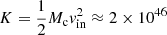 erg.
erg.
Although the kinetic energy carried by a single cloudlet may be substantial, it represents a transient energy injection. Given the average bolometric luminosity of the source ( ), the energy released by the accretion of a single clump would sustain the AGN output for only a few seconds (assuming efficient thermalization). Therefore, in order for this “raining” mechanism to have a significant, sustained impact on the global energy budget of the system, such accretion events cannot be sporadic. On the other hand, these cloudlets impacting the disk may play a crucial dynamical role beyond merely replenishing the fuel supply. The collision of such massive, dense clumps with the accretion disk may induce local instabilities and density perturbations within the flow. These stochastic inhomogeneities can then propagate inward through the disk on viscous timescales, effectively acting as the physical “seeds” for the propagating fluctuations model (e.g., Lyubarskii 1997; Arévalo & Uttley 2006). In this scenario, the raining material may contribute to the intrinsic variability of the accretion flow, providing a mechanism to explain the observed broadband timing properties, including the characteristic time lags detected between different X-ray energy bands (De Marco et al. 2013). It is finally worth mentioning here that the possible detection of a concurrent UFO signature in the form of an absorption line at E ∼ 7.3 keV (see also Ponti et al. 2009) is in agreement with the scenario depicted in Elvis (2017) for the formation of BLR in AGNs.
6. Conclusions
In this work, we presented a detailed spectral analysis of the Seyfert 1 galaxy Mrk 509, focusing on the high-resolution X-ray spectrum obtained by the XRISM/Resolve calorimeter, complemented by simultaneous NuSTAR and XMM-Newton observations. Our analysis leads to the following main conclusions:
-
The Fe K complex decomposition: Thanks to XRISM’s unprecedented resolution, we successfully disentangled the various components of the Fe K complex. We identified a narrow neutral Fe Kα core (σ < 10 eV), originating from distant material consistent with the dusty torus (as modeled by MYTorus). Additionally, we required a broad emission component and modeled it using either a broad Gaussian in emission or a relativistic reflection, revealing that it must originate at r ∼ 30 − 120 rg from the central engine, consistent with the BLR or the outer accretion disk rather than the innermost regions.
-
Partial covering versus pure relativistic reflection: We tested two scenarios to explain the spectral curvature and the 2–10 keV complexity. While a pure relativistic line can statistically reproduce the curvature, it yields a primary photon index (Γ ∼ 1.5 − 1.6, see Table 2) that is quite flat than the average values for Seyfert galaxies. Conversely, a partial covering model (for both models n8 and RR-n8 in Table 3) retrieves a canonical photon index (Γ ∼ 1.7 − 1.8).
-
Potential indications of a “raining” absorber: The modeling suggests the presence of an ionized partial absorber (log(ξ/erg cm s−1)∼2.5) which, under specific density assumptions (n ≈ 108 − 10 cm−3), is consistent with inflows at a high velocity of vin ≈ 11 000 km s−1. If confirmed, the physical modeling places this absorber at r ≈ 1100 − 1500 rg, consistent with a clumpy, fragmented flow. This is likely interpreted as “failed wind” clumps losing angular momentum and raining back toward the central black hole, possibly with a cometary-like shape.
Future monitoring with XRISM and NewAthena will be crucial to firmly confirm the existence and track the variability of these absorption features in Mrk 509 and in other sources. This is mandatory to firmly establish, if any, the possible connections between the infalling gas dynamics and the accretion flow that fuel the central SMBH in AGNs.
Acknowledgments
The authors are grateful to the anonymous referee for their careful reading of the manuscript and valuable feedback, which significantly strengthened this work. M.D., V.M., V.B., M.C., A.L., S.B., A.C., E.N., F.N., C.P., E.B. and A.T. acknowledge financial support from the Bando Ricerca Fondamentale INAF 2023, Large Program 1.05.23.01.06 (“The XRISM-to-XIFU (X2X) Agreement and Beyond: entering a new Era of High Resolution X-Ray Spectroscopy”). M.D, M.C. F.N and A.L. acknowledge financial support from PRIN MUR 2022 DRAGON 2022K9N5B4. E.B. acknowledges the support of the INAF GO grant “A JWST/MIRI MIRACLE: Mid-IR Activity of Circumnuclear Line Emission” and of the “Ricerca Fondamentale 2024” INAF program (mini-grant 1.05.24.07.01). P.O.P. acknowledges support from the CNES french spatial agency and from the ≪ Action Thématique Phénomèes Extrêmes et Multimessager ≫ of the Astronomy-Astrophysics National Programme from INSU/CNRS. C.P. is funded by INAF Large Grant 2023 BLOSSOM F.O. 1.05.23.01.13. R.S. acknowledges funding from the CAS-ANID grant number CAS220016.
References
- Akaike, H. 1974, IEEE Trans. Automat. Control, 19, 716 [Google Scholar]
- Antonucci, R. 1993, ARA&A, 31, 473 [Google Scholar]
- Arévalo, P., & Uttley, P. 2006, MNRAS, 367, 801 [Google Scholar]
- Arnaud, K., Dorman, B., & Gordon, C. 1999, Astrophysics Source Code Library [record ascl:9910.005] [Google Scholar]
- Barvainis, R. 1987, ApJ, 320, 537 [Google Scholar]
- Bianchi, S., Guainazzi, M., Matt, G., et al. 2009, A&A, 495, 421 [NASA ADS] [CrossRef] [EDP Sciences] [Google Scholar]
- Bianchi, S., Vander Meulen, B., Bertola, E., et al. 2026, A&A, 710, A294 [Google Scholar]
- Braito, V., Reeves, J. N., Matzeu, G. A., et al. 2018, MNRAS, 479, 3592 [Google Scholar]
- Brenneman, L. W., Wilkins, D. R., Ogorzałek, A., et al. 2025, ApJ, 995, 200 [Google Scholar]
- Cappi, M. 2006, Astron. Nachr., 327, 1012 [NASA ADS] [CrossRef] [Google Scholar]
- Cappi, M., Tombesi, F., Bianchi, S., et al. 2009, A&A, 504, 401 [NASA ADS] [CrossRef] [EDP Sciences] [Google Scholar]
- Chartas, G., Brandt, W. N., Gallagher, S. C., et al. 2002, ApJ, 579, 169 [Google Scholar]
- Chartas, G., Kochanek, C. S., Dai, X., et al. 2009, ApJ, 693, 174 [Google Scholar]
- Chartas, G., Cappi, M., Vignali, C., et al. 2021, ApJ, 920, 24 [NASA ADS] [CrossRef] [Google Scholar]
- Collin, S., Kawaguchi, T., Peterson, B. M., & Vestergaard, M. 2006, A&A, 456, 75 [NASA ADS] [CrossRef] [EDP Sciences] [Google Scholar]
- Dadina, M. 2007, A&A, 461, 1209 [NASA ADS] [CrossRef] [EDP Sciences] [Google Scholar]
- Dadina, M. 2008, A&A, 485, 417 [NASA ADS] [CrossRef] [EDP Sciences] [Google Scholar]
- Dadina, M., Cappi, M., Malaguti, G., et al. 2005, A&A, 442, 461 [NASA ADS] [CrossRef] [EDP Sciences] [Google Scholar]
- Dadina, M., Vignali, C., Cappi, M., et al. 2018, A&A, 610, L13 [NASA ADS] [CrossRef] [EDP Sciences] [Google Scholar]
- Dauser, T., Garcia, J., Parker, M. L., et al. 2014, MNRAS, 444, L100 [NASA ADS] [CrossRef] [Google Scholar]
- De Marco, B., Ponti, G., Cappi, M., et al. 2013, MNRAS, 431, 2441 [Google Scholar]
- Detmers, R. G., Kaastra, J. S., Steenbrugge, K. C., et al. 2011, A&A, 534, A38 [NASA ADS] [CrossRef] [EDP Sciences] [Google Scholar]
- Elvis, M. 2017, ApJ, 847, 56 [NASA ADS] [CrossRef] [Google Scholar]
- Fabian, A. C., Iwasawa, K., Reynolds, C. S., & Young, A. J. 2000, PASP, 112, 1145 [NASA ADS] [CrossRef] [Google Scholar]
- Fabian, A. C., Zoghbi, A., Ross, R. R., et al. 2009, Nature, 459, 540 [Google Scholar]
- Ferland, G. J., Korista, K. T., Verner, D. A., et al. 1998, PASP, 110, 761 [Google Scholar]
- García, J. A., Fabian, A. C., Kallman, T. R., et al. 2016, MNRAS, 462, 751 [Google Scholar]
- Gaspari, M., Tombesi, F., & Cappi, M. 2020, Nat. Astron., 4, 10 [Google Scholar]
- Ghisellini, G., Haardt, F., & Matt, G. 2004, A&A, 413, 535 [NASA ADS] [CrossRef] [EDP Sciences] [Google Scholar]
- Gianolli, V. E., Kim, D. E., Bianchi, S., et al. 2023, MNRAS, 523, 4468 [NASA ADS] [CrossRef] [Google Scholar]
- Gianolli, V. E., Bianchi, S., Petrucci, P.-O., et al. 2024, A&A, 687, A235 [NASA ADS] [CrossRef] [EDP Sciences] [Google Scholar]
- Giustini, M., & Proga, D. 2019, A&A, 630, A94 [NASA ADS] [CrossRef] [EDP Sciences] [Google Scholar]
- Giustini, M., Costantini, E., De Marco, B., et al. 2017, A&A, 597, A66 [NASA ADS] [CrossRef] [EDP Sciences] [Google Scholar]
- Gofford, J., Reeves, J. N., Tombesi, F., et al. 2013, MNRAS, 430, 60 [Google Scholar]
- Grafton-Waters, S., Branduardi-Raymont, G., Mehdipour, M., et al. 2021, A&A, 649, A120 [Google Scholar]
- GRAVITY Collaboration (Amorim, A., et al.) 2024, A&A, 684, A167 [NASA ADS] [CrossRef] [EDP Sciences] [Google Scholar]
- Haardt, F., & Maraschi, L. 1993, ApJ, 413, 507 [Google Scholar]
- Haardt, F., Maraschi, L., & Ghisellini, G. 1994, ApJ, 432, L95 [NASA ADS] [CrossRef] [Google Scholar]
- Harrison, F. A., Craig, W. W., Christensen, F. E., et al. 2013, ApJ, 770, 103 [Google Scholar]
- Heckman, T. M., & Best, P. N. 2014, ARA&A, 52, 589 [Google Scholar]
- Hölzer, G., Fritsch, M., Deutsch, M., Härtwig, J., & Förster, E. 1997, Phys. Rev. A, 56, 4554 [CrossRef] [Google Scholar]
- Huchra, J., Latham, D. W., da Costa, L. N., et al. 1993, AJ, 105, 1637 [NASA ADS] [CrossRef] [Google Scholar]
- Ishisaki, Y., Kelley, R. L., Awaki, H., et al. 2025, J. Astron. Telesc. Instrum. Syst., 11, 042023 [Google Scholar]
- Jansen, F., Lumb, D., Altieri, B., et al. 2001, A&A, 365, L1 [NASA ADS] [CrossRef] [EDP Sciences] [Google Scholar]
- Kaastra, J. S., Detmers, R. G., Mehdipour, M., et al. 2012, A&A, 539, A117 [NASA ADS] [CrossRef] [EDP Sciences] [Google Scholar]
- Kallman, T., & Bautista, M. 2001, ApJS, 133, 221 [Google Scholar]
- Kammoun, E., Kawamuro, T., Murakami, K., et al. 2025, ApJ, accepted [arXiv:2510.24971] [Google Scholar]
- King, A., & Pounds, K. 2015, ARA&A, 53, 115 [NASA ADS] [CrossRef] [Google Scholar]
- Kormendy, J., & Ho, L. C. 2013, ARA&A, 51, 511 [Google Scholar]
- Kumari, N., Pal, M., Naik, S., et al. 2021, PASA, 38, e042 [Google Scholar]
- Laha, S., Reynolds, C. S., Reeves, J., et al. 2021, Nat. Astron., 5, 13 [NASA ADS] [CrossRef] [Google Scholar]
- Li, Y.-R., Hu, C., Yao, Z.-H., et al. 2024, ApJ, 974, 86 [Google Scholar]
- Li, C., Kaastra, J. S., Gu, L., et al. 2026, A&A, 706, A255 [NASA ADS] [CrossRef] [EDP Sciences] [Google Scholar]
- Longinotti, A. L., Sim, S. A., Nandra, K., et al. 2007, MNRAS, 374, 237 [Google Scholar]
- Lyubarskii, Y. E. 1997, MNRAS, 292, 679 [Google Scholar]
- Maiolino, R., Risaliti, G., Salvati, M., et al. 2010, A&A, 517, A47 [NASA ADS] [CrossRef] [EDP Sciences] [Google Scholar]
- Mao, J., Kaastra, J. S., Mehdipour, M., et al. 2017, A&A, 607, A100 [NASA ADS] [CrossRef] [EDP Sciences] [Google Scholar]
- Marinucci, A., Muleri, F., Dovciak, M., et al. 2022, MNRAS, 516, 5907 [NASA ADS] [CrossRef] [Google Scholar]
- Matzeu, G. A., Reeves, J. N., Nardini, E., et al. 2016, MNRAS, 458, 1311 [Google Scholar]
- Matzeu, G. A., Reeves, J. N., Braito, V., et al. 2017, MNRAS, 472, L15 [NASA ADS] [CrossRef] [Google Scholar]
- Matzeu, G. A., Brusa, M., Lanzuisi, G., et al. 2023, A&A, 672, A24 [NASA ADS] [CrossRef] [EDP Sciences] [Google Scholar]
- Mehdipour, M., Branduardi-Raymont, G., Kaastra, J. S., et al. 2011, A&A, 534, A39 [NASA ADS] [CrossRef] [EDP Sciences] [Google Scholar]
- Mehdipour, M., Kaastra, J. S., Eckart, M. E., et al. 2025, A&A, 699, A228 [NASA ADS] [CrossRef] [EDP Sciences] [Google Scholar]
- Middei, R., Bianchi, S., Petrucci, P. O., et al. 2019, MNRAS, 483, 4695 [NASA ADS] [CrossRef] [Google Scholar]
- Mizumoto, M., Reeves, J. N., Braito, V., et al. 2026, ApJ, 997, 219 [Google Scholar]
- Murphy, K. D., & Yaqoob, T. 2009, MNRAS, 397, 1549 [Google Scholar]
- Nandra, K., & Pounds, K. A. 1994, MNRAS, 268, 405 [Google Scholar]
- Nandra, K., George, I. M., Mushotzky, R. F., et al. 1999, ApJ, 523, L17 [Google Scholar]
- Nandra, K., O’Neill, P. M., George, I. M., & Reeves, J. N. 2007, MNRAS, 382, 194 [NASA ADS] [CrossRef] [Google Scholar]
- Nardini, E., Reeves, J. N., Gofford, J., et al. 2015, Science, 347, 860 [Google Scholar]
- Negrete, C. A., Dultzin, D., Marziani, P., et al. 2012, ApJ, 757, 62 [NASA ADS] [CrossRef] [Google Scholar]
- Pal, I., Stalin, C. S., Chatterjee, R., et al. 2023, JApA, 44, 87 [NASA ADS] [Google Scholar]
- Peca, A., Koss, M. J., Serafinelli, R., et al. 2025, ApJ, 989, 84 [Google Scholar]
- Peterson, B. M., Ferrarese, L., Gilbert, K. M., et al. 2004, ApJ, 613, 682 [Google Scholar]
- Petrucci, P.-O., Paltani, S., Malzac, J., et al. 2013, A&A, 549, A73 [NASA ADS] [CrossRef] [EDP Sciences] [Google Scholar]
- Petrucci, P.-O., Ursini, F., De Rosa, A., et al. 2018, A&A, 611, A59 [NASA ADS] [CrossRef] [EDP Sciences] [Google Scholar]
- Piconcelli, E., Jimenez-Bailón, E., Guainazzi, M., et al. 2005, A&A, 432, 15 [NASA ADS] [CrossRef] [EDP Sciences] [Google Scholar]
- Ponti, G., Cappi, M., Vignali, C., et al. 2009, MNRAS, 394, 1487 [NASA ADS] [CrossRef] [Google Scholar]
- Ponti, G., Cappi, M., Costantini, E., et al. 2013, A&A, 549, A72 [NASA ADS] [CrossRef] [EDP Sciences] [Google Scholar]
- Pounds, K., Reeves, J., O’Brien, P., et al. 2001, ApJ, 559, 181 [NASA ADS] [CrossRef] [Google Scholar]
- Pounds, K. A., Reeves, J. N., King, A. R., et al. 2003, MNRAS, 345, 705 [Google Scholar]
- Proga, D., & Kallman, T. R. 2004, ApJ, 616, 688 [Google Scholar]
- Ramos Almeida, C., & Ricci, C. 2017, Nat. Astron., 1, 679 [Google Scholar]
- Reeves, J. N., Wynn, G., O’Brien, P. T., et al. 2002, MNRAS, 335, 126 [Google Scholar]
- Reeves, J. N., O’Brien, P. T., Braito, V., et al. 2009, ApJ, 701, 493 [NASA ADS] [CrossRef] [Google Scholar]
- Reeves, J. N., Braito, V., Gofford, J., et al. 2014, ApJ, 780, 45 [Google Scholar]
- Reeves, J. N., Braito, V., Nardini, E., et al. 2018, ApJ, 854, L8 [NASA ADS] [CrossRef] [Google Scholar]
- Ricci, C., Trakhtenbrot, B., Koss, M. J., et al. 2017, ApJS, 233, 17 [Google Scholar]
- Risaliti, G., Elvis, M., Fabbiano, G., et al. 2007, ApJ, 659, L111 [NASA ADS] [CrossRef] [Google Scholar]
- Risaliti, G., Nardini, E., Salvati, M., et al. 2011, MNRAS, 410, 1027 [Google Scholar]
- Ross, R. R., & Fabian, A. C. 1993, MNRAS, 261, 74 [NASA ADS] [CrossRef] [Google Scholar]
- Serafinelli, R., Tombesi, F., Vagnetti, F., et al. 2019, A&A, 627, A121 [NASA ADS] [CrossRef] [EDP Sciences] [Google Scholar]
- Shakura, N. I., & Sunyaev, R. A. 1973, A&A, 24, 337 [NASA ADS] [Google Scholar]
- Śniegowska, M., Marziani, P., Czerny, B., et al. 2021, ApJ, 910, 115 [CrossRef] [Google Scholar]
- Tanaka, Y., Nandra, K., Fabian, A. C., et al. 1995, Nature, 375, 659 [NASA ADS] [CrossRef] [Google Scholar]
- Tashiro, M., Watanabe, S., Maejima, H., et al. 2024, Proc. SPIE, 13093, 130931G [Google Scholar]
- Tashiro, M., Kelley, R., Watanabe, S., et al. 2025, PASJ, 77, S1 [Google Scholar]
- Tombesi, F., Cappi, M., Reeves, J. N., et al. 2010, A&A, 521, A57 [NASA ADS] [CrossRef] [EDP Sciences] [Google Scholar]
- Tombesi, F., Cappi, M., Reeves, J. N., et al. 2011, ApJ, 742, 44 [Google Scholar]
- Tombesi, F., Cappi, M., Reeves, J. N., et al. 2013, MNRAS, 430, 1102 [Google Scholar]
- Wilkins, D. R., & Fabian, A. C. 2011, MNRAS, 414, 1269 [CrossRef] [Google Scholar]
- XRISM Collaboration (Audard, M., et al.) 2024, ApJ, 973, L25 [Google Scholar]
- Xrism Collaboration (Audard, M., et al.) 2025a, Nature, 641, 1132 [Google Scholar]
- Xrism Collaboration (Audard, M., et al.) 2025b, A&A, 702, A147 [Google Scholar]
- Yaqoob, T. 2012, MNRAS, 423, 3360 [Google Scholar]
- Yaqoob, T., & Murphy, K. D. 2011, MNRAS, 412, 277 [Google Scholar]
- Yaqoob, T., & Padmanabhan, U. 2004, ApJ, 604, 63 [NASA ADS] [CrossRef] [Google Scholar]
- Yaqoob, T., & Serlemitsos, P. 2005, ApJ, 623, 112 [Google Scholar]
- Yaqoob, T., McKernan, B., Kraemer, S. B., et al. 2003, ApJ, 582, 105 [Google Scholar]
- Zhao, X., Civano, F., Fornasini, F. M., et al. 2021, MNRAS, 508, 5176 [NASA ADS] [CrossRef] [Google Scholar]
All Tables
All Figures
|
Fig. 1. Time scheme of the X-ray observation presented in this work. The horizontal lines represent the total observation times. |
| In the text | |
|
Fig. 2. Non-background-subtracted XRISM/Resolve light curves of Mrk 509 shown in the 2–5 keV (top panel) and 5–12 keV (middle panel) energy bands. Bottom: Corresponding hardness ratio. A clear brightening trend is evident toward the end of the observation, but it is not accompanied by significant spectral variability. |
| In the text | |
|
Fig. 3. Upper panel: 2–60 keV ratio between the data and a simple power-law model for the Mrk 509 X-ray data taken during this campaign (see Table 1), expressed in units of standard deviations. Here, for clarity purposes, the data have been strongly rebinned (each data point has a 25σ significance). Lower panel: 2–12 keV spectrum of Mrk 509 observed by XRISM/Resolve. The orange line represents the best fit using a simple power-law model. In this case, the Resolve data have also been rebinned (each data point here has a significance of 15σ) for visual clarity. |
| In the text | |
|
Fig. 4. Upper panel: Residuals of the PC2 model (neutral partial covering with distant reflection component). Lower panel: Residuals of the RR2 model (neutral partial covering with a relativistic reflection component and narrow Fe Kα Gaussian emission line). In all panels, the XMM-Newton data are in red, while the NuSTAR data are in blue. |
| In the text | |
|
Fig. 5. Zoom-in on the 5.5–7.5 keV range PC2 model (see Table 2). XMM-Newton data observation 1 is in black, observation 2 is in red, and observation 3 is in magenta. The NuSTAR data are in gray. There are no significant residuals. |
| In the text | |
|
Fig. 6. 5–7.5 keV zoom-in on the Resolve residuals for the model including cold partial covering and the zFeKlor component to account for the narrow Fe Kα complex. The data are strongly rebinned for clarity purposes (each data point in the plot has a 20σ significance). The most significant deviations from the model are a possible absorption feature at E ∼ 6.2 keV and a broader component in the 6–6.8 keV range. |
| In the text | |
|
Fig. 7. Confidence contours between the column density and broadening kernel for the distant reflector from MYTorus modeling of the reflector and associated lines (see Sect. 4.1). |
| In the text | |
|
Fig. 8. 2–12 keV spectrum of Mrk 509 modeled with partial covering of the primary emission, broad Gaussian line, and neutral reflection (MYTorus model; see model I in Table 3). The components are shown as dotted lines: absorbed power-law (red), absorbed broad Gaussian line (blue), MYTorusL (magenta), and MYTorusS (orange). |
| In the text | |
|
Fig. 9. Upper panel: Confidence contours (rest-frame energies) from the blind search for possible absorption features (see Sect. 4.2). Lower panel: Zoom-in on the spectral range where the strongest feature (absorption line at |
| In the text | |
|
Fig. 10. 6.0–6.8 keV zoom-in on the spectral range where the strongest features from ionized gas are measured (model n8 in Table 3). The features measured in the 6.1–6.4 keV range are due to the Fe XVIII–Fe XXI lines. |
| In the text | |
|
Fig. 11. Upper panel: 99%, 90%, and 68% confidence contours for the z vs. NH parameters obtained using model n8 in Table 3. |
| In the text | |
|
Fig. 12. Cumulative distribution of the ΔC statistic derived from 1500 Monte Carlo simulations, assuming Model I (see Table 2) as the null hypothesis. Synthetic XRISM/Resolve spectra were generated matching the exposure time of the real observation. For each simulation, ΔC is defined as the difference in the C-statistic between the best fits obtained modeling the simulated datasets with Model I and Model n8 in Table 2. The vertical green line indicates the mean simulated ΔC, while the red line marks the 3σ confidence threshold. The purple line represents the ΔC value observed in the real data. |
| In the text | |
Current usage metrics show cumulative count of Article Views (full-text article views including HTML views, PDF and ePub downloads, according to the available data) and Abstracts Views on Vision4Press platform.
Data correspond to usage on the plateform after 2015. The current usage metrics is available 48-96 hours after online publication and is updated daily on week days.
Initial download of the metrics may take a while.