


| Issue |
A&A
Volume 710, June 2026
|
|
|---|---|---|
| Article Number | A28 | |
| Number of page(s) | 20 | |
| Section | Astrophysical processes | |
| DOI | https://doi.org/10.1051/0004-6361/202556995 | |
| Published online | 29 May 2026 | |
XRISM reveals a variable, multi-phase outflow-inflow structure during the 2024 X-ray obscured outburst of black hole transient V4641 Sgr
1
Department of Physics, Ehime University, 2-5, Bunkyocho, Matsuyama, Ehime 790-8577, Japan
2
Department of Earth and Space Science, Graduate School of Science, Osaka University, 1-1 Machikaneyama, Toyonaka, Osaka 560-0043, Japan
3
Centre for Extragalactic Astronomy, Department of Physics, University of Durham, South Road, Durham DH1 3LE, UK
4
Instituto de Astrofísica de Canarias, E-38205 La Laguna, Tenerife, Spain
5
Departamento de Astrofísica, Universidad de La Laguna, E-38206 La Laguna, Tenerife, Spain
6
Institute of Space and Astronautical Science (ISAS), Japan Aerospace Exploration Agency (JAXA), Kanagawa 252-5210, Japan
7
Institute of Space Sciences (ICE, CSIC), Campus UAB, Carrer de Can Magrans s/n, E-08193 Barcelona, Spain
8
Institut d’Estudis Espacials de Catalunya (IEEC), 08860 Castelldefels (Barcelona), Spain
9
INAF/IASF Palermo, Via Ugo La Malfa 153, I-90146 Palermo, Italy
10
Université Paris Cité and Université Paris Saclay, CEA, CNRS, AIM, F-91190 Gif-sur-Yvette, France
11
Departamento de Física, CUCEI, Universidad de Guadalajara, 44430 Guadalajara, Jalisco, Mexico
12
Doctorado en Ciencias Fisico-Matematicas, CUValles, Universidad de Guadalajara, Carretera Guadalajara–Ameca km. 45.5, 46600 Ameca, Jalisco, Mexico
13
National Astronomical Observatories, Chinese Academy of Sciences, 20A Datun Road, Beijing 100101, China
14
ESO, Karl-Schwarzschild-Strasse 2, 85748 Garching bei München, Germany
15
Department of Physics, University of Oxford, Denys Wilkinson Building, Keble Road, Oxford OX1 3RH, UK
16
Department of Astronomy, University of Cape Town, Private Bag X3, Rondebosch 7701, South Africa
17
Okayama Observatory, Kyoto University, 3037-5 Honjo, Kamogatacho, Asakuchi, Okayama 719-0232, Japan
18
Department of Multi-Disciplinary Sciences, Graduate School of Arts and Sciences, The University of Tokyo, 3-8-1 Komaba, Meguro, Tokyo 153-8902, Japan
19
Department of Physics, Tokyo University of Science, 1-3 Kagurazaka, Shinjuku-ku, Tokyo 162-8601, Japan
20
Istituto Nazionale di Astrofisica, Osservatorio Astronomico di Brera, Via E. Bianchi 46, 23807 Merate, (LC), Italy
21
Department of Physics, Nihon University, 1-8 Kanda-Surugadai, Chiyoda-ku, Tokyo 101-8308, Japan
22
University of Manitoba, Winnipeg, MB R3T 2N2, Canada
23
Institute for Cosmic Ray Research, University of Tokyo, 5-1-5, Kashiwa-no-ha, Kashiwa, Chiba 277-8582, Japan
24
Interdisciplinary Theoretical & Mathematical Science Center (iTHEMS), RIKEN, 2-1, Hirosawa, Wako, Saitama 351-0198, Japan
25
Department of Astronomy, Kyoto University, Kitashirakawa-Oiwake-cho, Sakyo-ku, Kyoto, Kyoto 606-8502, Japan
26
Department of Physics, Missouri University of Science and Technology, Rolla, MO, USA
27
Center for Astrophysics, Harvard & Smithsonian, 60 Garden St, Cambridge, MA 02138, USA
28
Kapteyn Astronomical Institute, University of Groningen, P.O. BOX 800, 9700 AV, Groningen, The Netherlands
29
Astrophysics, Department of Physics, University of Oxford, Oxford OX1 3RH, UK
★ Corresponding authors: This email address is being protected from spambots. You need JavaScript enabled to view it.
, This email address is being protected from spambots. You need JavaScript enabled to view it.
Received:
26
August
2025
Accepted:
22
February
2026
Abstract
We report the results of a simultaneous X-ray and optical spectroscopy campaign on the Galactic black hole X-ray binary (BH XRB) V4641 Sgr, carried out with XRISM and the Seimei telescope during a low-luminosity phase toward the end of its 2024 outburst. Despite a very low X-ray luminosity of 1034 erg s−1, the continuum spectrum is well reproduced by a disk blackbody model with a high inner disk temperature (1.8 keV). XRISM/Resolve provides the highest resolution X-ray spectrum ever obtained from the source. Several strong, narrow emission lines have been detected, resolved, and characterized at a high significance. The continuum shape and narrow emission lines both indicate that the inner disk region is obscured by the surrounding high-density gas, while the intrinsic luminosity is at least one order of magnitude higher. In the simultaneous optical observation from the Seimei telescope, the line features are largely dominated by the optical companion. Although we detected a clear emission component in Hα that could originate from a cold outflow or the disk atmosphere, there are no signs of the strong outflow signatures historically detected in this source. In X-rays, the combination of significantly redshifted (∼700 km s−1) and weakly blueshifted (∼ − 250 km s−1) components, all varying strongly on kilosecond timescales, along with a marginally significant (99.2%) highly blueshifted (∼ − 1300 km s−1) component, indicating a complex, inhomogeneous outflow geometry. This is corroborated by the erratic long-term evolution of the source seen in the complementary X-ray monitoring, as well as radio detections spanning several orders of magnitude.
Key words: accretion, accretion disks / atomic processes / stars: black holes / stars: winds / outflows / X-rays: binaries
Invited Project Professor at Institute of Cosmic Ray Research, The University of Tokyo on June–July 2025.
© The Authors 2026
 Open Access article, published by EDP Sciences, under the terms of the Creative Commons Attribution License (https://creativecommons.org/licenses/by/4.0), which permits unrestricted use, distribution, and reproduction in any medium, provided the original work is properly cited.
This article is published in open access under the Subscribe to Open model. This email address is being protected from spambots. You need JavaScript enabled to view it. to support open access publication.
1. Introduction
X-ray binaries (XRBs) are a subcategory of X-ray sources, corresponding to one of the many evolutionary pathways of binary stellar systems when mass transfer from a main sequence “companion” star onto a stellar mass compact object leads to intense emission along the entire electromagnetic spectrum (and particularly in the X-ray). The dynamics of these systems, particularly those hosting a black hole (BH) or a neutron star (NS), strongly depend on the mass and behavior of the companion. In low-mass XRBs (LMXBs; Bahramian & Degenaar 2023), the evolution of a low-mass (≲1 M⊙) star and the binary system itself will trigger mass transfer through Roche Lobe overflow, leading to the formation of an accretion disk around the compact object. On the other hand, high-mass XRBs (HMXBs; Fornasini et al. 2024) host a B or O-type supergiant of a few or more solar masses and tend to feed the compact object directly with intense stellar winds. The majority of BH LMXBs, along with part of the HMXB population, is made of transients, exhibiting rare, erratically repeating periods where accretion and X-ray emission intensify for a few months to a few years and become detectable (i.e., so-called outbursts). The remaining time is spent in quiescence, at low accretion levels and negligible luminosities.
These outburst patterns display a coherent evolution through distinct spectral-timing states (see, e.g., Remillard & McClintock 2006; Done et al. 2007 in X-rays and Fender 2003 in the radio band). The onset is characterized by a rise in luminosity of more than five orders of magnitude through the hard state (HS), defined by a spectral cut-off power law peaking at ∼100 keV, originating in a hot, horizontally extended (Krawczynski et al. 2022) plasma region near the BH called the corona. In addition, there is a steady radio emission observed at gigahertz (GHz) radio frequencies with a flat synchrotron spectrum, likely produced by a compact, optically thick jet. Strong and rapid X-ray variability (up to 50% rms) is observed on time scales between 10 ms and 100 s, with characteristic frequencies (often manifested as quasi-periodic oscillations, QPOs, Ingram & Motta 2019) increasing with luminosity. Then, once a critical luminosity between ∼1 − 10% LEdd is surpassed, the spectrum begins to soften. A hitherto secondary component tracing an optically thick disk becomes dominant and extends close to or at the innermost stable circular orbit (ISCO), while the power law steepens and fades away, as the corona mostly disappears. During this hard-to-soft transition, the source shows major radio flares linked to transient, optically thin ejecta before the radio emission gets quenched, indicating a cessation of core jet activity. The source then remains in this soft, disk-dominated state (SS), with inner temperatures of kTin ∼ 1 − 1.5 keV and low variability, then fading to lower luminosities over the course of a few weeks to months. Once it goes below a precise Eddington ratio threshold (Vahdat Motlagh et al. 2019; Wang et al. 2023), the source transits back to the HS and the jet reappears as the emission continues to fade down to quiescence.
In addition to the continuum evolution, the last two decades have seen a series of discoveries of blueshifted, narrow, highly ionized absorption features in X-rays (i.e., mainly ionized iron lines from Fe XXV and/or Fe XXVI) in transient XRBs (Ueda et al. 1998; Kotani et al. 2000; Lee et al. 2002). These features trace hot and massive outflows that are dynamically important for the evolution of these systems. This is due to the removal of a substantial fraction of the disk mass or heating of the disk surface by scattering X-ray flux down onto the disk (Tetarenko et al. 2018a; Dubus et al. 2019; Tetarenko et al. 2020; Ponti et al. 2016; Tetarenko et al. 2018b). Only high-inclination (dipping) sources show such powerful “hot” winds, likely due to the equatorial nature of these outflows. Moreover, in X-rays, these winds are generally detected during the SS (e.g., Ponti et al. 2012; Parra et al. 2024) and remain undetected during the HS. The fact that the “hot” wind signatures disappear during the HS is likely related to photoionization instability of the wind in the ionization domain consistent with the presence of Fe XXV and Fe XXVI in that state (Chakravorty et al. 2013; Bianchi et al. 2017 but see Gatuzz et al. 2019). However, the shapes of these stability curves are strongly dependent on the spectral shape of the ionizing spectral energy distribution (SED, Chakravorty et al. 2013; Bianchi et al. 2017; Petrucci et al. 2021; Parra et al. 2025).
Still, the picture is more complicated than a simple on-off wind process between spectral states. Recent results pertaining to the (hard and soft) intermediate states (HIS and SIS, respectively) that are characteristic of the hard-soft state transition, reveal a wide variety of X-ray wind properties and signatures (Miller et al. 2008; Kallman et al. 2009; Neilsen et al. 2016; Shidatsu et al. 2016; Muñoz-Darias et al. 2017; Gatuzz et al. 2019). In parallel, recent observations in the optical and infrared (OIR) range (Jiménez-Ibarra et al. 2019; Muñoz-Darias et al. 2019; Mata Sánchez et al. 2022; Sánchez-Sierras et al. 2023) have indicated the presence of low ionization absorption features during the entirety of the outbursts. Whether these “cold” winds are different from the “hot” ones (or both end up being the same component but seen through different ionization states) is still highly debated, notably due to the lack of simultaneous wind detections in different wavelengths in standard systems (Muñoz-Darias & Ponti 2022; Parra et al. 2024).
V4641 Sgr is a transient galactic X-ray binary located at 6.2 ± 0.7 kpc. It consists of a BH with a mass of 6.4 ± 0.6 M⊙ and a B9III companion with 2.9 ± 0.4 M⊙ (MacDonald et al. 2014) orbiting each other with a period of 2.82 days (Orosz et al. 2001; Uemura et al. 2002). The source was identified as an X-ray source due to a giant outburst in 1999 (Smith et al. 1999; Hjellming et al. 2000; Stubbings et al. 1999). Since then, it has shown a dozen smaller outbursts, with a reccurence interval of 2−4 years (Tetarenko et al. 2016). The source is also one of the several BH XRBs around which diffuse emission in the TeV gamma-ray band has been detected (Alfaro et al. 2024; Cao et al. 2025) and for which a possible X-ray counterpart was recently discovered using XRISM/Xtend (Suzuki et al. 2025).
During its outbursts, the spectral evolution of the source remains completely different from the classical Q-shape evolution and spectral states seen in standard outbursting BHXRBs (see, e.g., Dunn et al. 2010). It either shows a hard, reflection-dominated spectrum (Morningstar et al. 2014) or a disk blackbody spectrum (Pahari et al. 2015; Bahramian et al. 2015; Shaw et al. 2022), both at very low luminosities, typically below L/LEdd ∼ 10−3. These unusual spectral states suggest that the outer disk or its atmosphere completely obscures the inner regions of the accretion flow and that the observed flux is only a tiny fraction of the central source revealed by scattering and photoionized emission from the X-ray heated disk atmosphere or wind. In the disk-dominated state, several narrow, highly ionized emission lines, including Fe XXVI Lyα (also referred to as Fe XXVI Kα) and Fe XXV Heα (also referred to as Fe XXV Kα), were first discovered with Chandra/HETG in 2020 (Shaw et al. 2022). In these spectra, the iron emission lines showed negligible velocity shifts, but a lower ionized layer, with marginal (uncorrected) blueshifts in absorption and marginal redshifts in emission, was also detected from the lines of less massive elements. The former can retroactively explain the iron line feature seen at lower spectral resolution in soft state NuSTAR observations of previous outbursts (Pahari et al. 2015). The presence of a high-speed, “cold”, low ionized wind (first associated with the September 1999 X-ray outburst and later with subsequent outbursts) was first suspected from the complex emission profiles seen in optical spectroscopy (Charles et al. 1999; Chaty et al. 2003; Lindstrøm et al. 2005). It was later unambiguously confirmed with P-Cygni profiles and blueshifted absorption lines (Muñoz-Darias et al. 2018), with terminal velocities of several 1000 km s−1. However, the association between these strong optical wind signatures and a potential “hot”, highly ionized wind phase, which has yet to be directly identified, remains unclear.
A new outburst of V4641 Sgr was detected on 2024 September 6 (Negoro et al. 2024), three years after the previous outburst. To better determine the properties and profiles of the emission lines, which were only partly constrained by the previous Chandra observations, we observed the source with XRISM (Tashiro et al. 2020), as the first Director’s Discretionary Time (DDT) observation of the mission since the beginning of the guest observer phase. We also performed simultaneous optical spectroscopy with the 3.8-m Seimei telescope in Japan to search for optical wind signatures.
In this paper, we present the results of our spectral analysis of both datasets, complemented by the publicly available X-ray monitoring of this outburst using MAXI, NICER, and Swift, as well as the coverage of Einstein Probe, along with reports from radio monitoring using MeerKAT. We describe our observations and the data reduction procedures in Section 2 and the results of the X-ray spectral analysis in Section 3. Section 4 describes our analysis of the optical observation. In Section 5, we discuss these results, particularly in the context of the obscuration of the source and its possible outflow structure. Our conclusions are given in Section 6. Appendix A details the velocity correction applied to our X-ray spectra. Appendices B–D offer complementary information on the monitoring, data reduction, and spectral analysis methodologies used in this work. In addition, we provide the full results of the blind searches for time-averaged and time-resolved spectra derived in our analysis in an online format in Appendix E.
2. Observation and data reduction
2.1. XRISM
The XRISM observation of V4641 Sgr was carried out on 2024 September 30 UT 09:41−17:02 (OBSID 901001010), with a net exposure of ∼13 ks. During the observation, the microcalorimeter Resolve (Ishisaki et al. 2022) was operated with no filters and the soft X-ray imager Xtend (Mori et al. 2022; Noda et al. 2025; Uchida et al. 2025) was operated in the full window mode. As shown in Figure 1, the source exhibited flaring activity for a few days in early September and then a rapid flux drop was seen. The observation was executed at the end of the outburst, close to quiescence. We note that while the MAXI evolution appears to follow the results of the NICER and Swift monitoring, the flux values derived from MAXI (both with the on-demand tool and PSF-fitting) remain higher than those obtained with direct fitting from NICER and Swift. The brightest Swift observation had a 1−10 keV flux of ∼2 × 10⁻¹⁰ erg s−1 cm−2, while the MAXI flux values were overestimated by a factor ≳3. This is likely because the flux values in the MAXI data are converted from the count rates by assuming the spectrum of the Crab Nebula. The data were reduced with Heasoft version 6.34 and the latest version of the XRISM Calibration Database as of the observation date, following the XRISM Quick Start Guide v2.31.
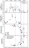 |
Fig. 1. Long-term monitoring of V4641 Sgr with different instruments during the 2024 outburst. From top to bottom: (first) MAXI daily light curve in the 2–10 keV band, obtained via PSF fitting (black), and generated via the MAXI on-demand interface (gray). See Sect. 2.2.1 for details. (Second) Einstein probe light curve in the 0.5–4 keV band. (Third) NICER/Swift/XRISM 1–10 keV luminosity light curves in Eddington units, after removal of the ISM absorption component. (Fourth) NICER/Swift/XRISM 6–10/3–10 keV hardness ratio (HR) evolution. The results in the last two panels come from fitting the time-integrated spectra of the individual ObsIDs in this period (see Sect. 2.2 for more details). The blue and red lines highlight the radio observations reported in Grollimund et al. (2024a,b), and the green line the XRISM and simultaneous Seimei observations. |
2.1.1. Resolve
The energy scale was measured using a set of 55Fe sources on the filter wheel, which illuminated the entire array at fiducial time intervals selected to follow the characteristic pattern of gain changes caused by the cycles of the 50 mK cooler. The Mn Kα line complex from 55Fe was fitted for each fiducial interval and pixel using an eight-component model with intrinsic Lorentzian profiles, which were convolved with Gaussian smoothing to account for the detector’s resolution. The energy scale was corrected by nonlinear interpolation between gain curves measured at different heat-sink temperatures and linear interpolation between the fiducial measurements. Out of the 36 pixels in the Resolve detector, 35 pixels were usable for scientific purposes and the last one is a calibration pixel. Since random gain jumps of unknown origin, lasting approximately 1−2 hours, were observed for pixel 27 and the current fiducial strategy was unable to track these gain jumps, data from pixel 27 were excluded. Gaussian modeling of line spread of the detector for the Mn Kα line indicated a resolution of 4.45 ± 0.04 eV FWHM, with an energy shift of 0.0071 ± 0.0182 eV2. Early calibration measurements showed that the energy scale was accurate to within approximately ±1 eV over the 2−8 keV range (Porter et al. 2024; Eckart et al. 2024). We applied an additional screening of the standard energy-dependent rise time cut (Mochizuki et al. 2025), and restricted ourselves to high-resolution primary (Hp) events.
The response matrix file (RMF) was generated with rslmkrmf. Its normalization was computed according to the fraction of events with the relevant grade in the cleaned event file. However, at low count rates, Resolve’s cleaned event files can include a significant fraction of low-resolution secondary (Ls) events that are not due to the source, but instead result from the secondary-pulse detection algorithm on clipped pulses. To assess the degree of Ls event contamination, we computed both the theoretical and observed branching ratios (proportion of events in each grade) of each pixel in the observation. We show the result in Fig. C.1. In pixel 18, the brightest pixel of the observation, the combined branching ratio of all medium- and low-resolution events should be less than 0.8%. The entire observation should thus have a Hp grade branching ratio of virtually 100%. Yet, we see a nonnegligible contribution (between a few percent and a few tens of percent) of Ls events, with values between one and three orders of magnitude above theoretical expectations, which confirms the high degree of Ls contamination. Thus, we removed the Ls events from the cleaned event file before calculating the RMF. On the other hand, the Mp (middle-resolution primary), Ms (middle-resolution secondary), and Lp (low-resolution primary) contribution, despite being higher than normal, remained negligible and did not affect our analysis. The ancillary response file (ARF) was generated with xaarfgen assuming a point-like source at the aim point as input. To produce the spectrum, we adapted an energy range of 2−12 keV, below which the X-ray signals are mostly absorbed by the closed gate valve. We generated the non-X-ray background (NXB) file using rslnxbgen task, excluding pixel 27 and using only the Hp events. The NXB spectrum was fitted with the model provided by the XRISM Calibration team, consisting of a power law and instrumental emission lines presented by 17 narrow positive Gaussians: Al Kα1/Kα2, Au Mα1, Cr Kα1/Kα2, Mn Kα1/Kα2, Fe Kα1/Kα2, Ni Kα1/Kα2, Cu Kα1/Kα2, Au Lα1/Lα2, and Au Lβ1/Lβ2.
2.1.2. Xtend
The time-averaged source spectra were extracted from a circular region with a radius of 2.5 arcmin centered on the source peak and the background from a source-free circular region with the same radius. The RMF and ARF were generated with xtdrmf and xaarfgen, respectively. We used the 0.4−12 keV band, as above and below these values, the source count rates become lower than the background rates.
2.2. X-ray monitoring
2.2.1. MAXI
Due to the very limited flux of the source during the outburst, data from the MAXI (Matsuoka et al. 2009) all-sky monitoring instruments must be analyzed carefully. We thus computed the MAXI light curve in the 2−10 keV band using two methods. First, we used an updated PSF fitting, following the method in Morii et al. (2016), which uses the well-calibrated cameras (Camera ID: 2, 4, 5, and 7) and considering the contribution of nearby sources, including GS 1826−238, GX 5−1, and NGC 6624. Second, for comparison, we generated light curve products using the MAXI on-demand interface3 (gray), with an improved methodology (Nakahira et al. 2012) compared to the standard products provided directly on the standard website4. The results are shown in the top panel of Fig. 1.
2.2.2. NICER
The Neutron Star Interior Composition Explorer (NICER; Gendreau et al. 2016) began observing the source soon after the first report of the 2024 outburst from Negoro et al. (2024). We analyzed every observation of this last outburst, using an automated data reduction procedure based on the NICERDAS software5 version 12, with the latest calibration files available (CADLB ver:xti20240206). To use the scorpeon background model, we downloaded geomagnetic data using the NICERDAS task nigeodown. We split the data into continuous observation periods for each day, filtered them to remove background flares following the procedures detailed in the NICER data analysis threads6, and extracted spectra using the nicerl3-spect task of NICERDAS. We used the xspec-model version of the scorpeon background model, which is important to better constrain the background contribution in such faint observations. All spectra were grouped following the optimized binning of Kaastra & Bleeker (2016).
We performed spectral analysis independently on each of the 25 days of observation, further splitting the individual observation periods of each day when their count rate in the 3−8 keV band or their hardness ratio in the 5−8/3−5 keV band changed by more than 20%. We removed observation periods where very low exposures of high background contamination prevented a good spectral fitting. The resulting 30 epochs were fit in the 0.3−10 keV band, with an absorbed comptonized disk model, using phabs*Tbabs*thcomp*diskbb. We set interstellar medium (ISM) abundances to wilm (Wilms et al. 2000) and the ISM column density (in TBabs) was fixed at 1.5 ⋅ 1021 cm−2, following our results for the XRISM analysis (see Sect. 3). The second phabs absorption component was left free to account for the additional absorber intrinsic to the source and varied between 0 and NH ∼ 3 ⋅ 1021 cm−2 between observations. We note that the choice of phabs is mainly to highlight the intrinsic nature of this second source of absorption and in contrast to TBabs. The choice of component to represent each absorption layer does not impact the fits at the current signal-to-noise ratio (S/N). The electron temperature of the Comptonization component was fixed at 100 keV. For each epoch, we then derived the unabsorbed 1−10 keV flux, the 6−10 keV/3−10 keV hardness ratio, and their 90% uncertainties. In order to facilitate the comparison between observations, and due to the highly unknown nature of the intrinsic absorber, we only removed the fixed ISM absorption component (TBabs) to effectively show the absorbed intrinsic luminosity of the source in the bottom panels of Fig. 1. The source remained very soft and relatively stable over ∼2 weeks (between September 7, the date of the first NICER observation, and September 24). Although a detailed spectral analysis of the NICER observations is beyond the scope of this paper, we note that the spectra were perfectly fit with a thermal disk, with a temperature of ∼1.1 − 1.2 keV, and up to two highly variable narrow emission lines between 6.4 and 7 keV. Then, after an extremely erratic ∼3 week period during which both the hardness ratio and luminosity vary intensely down to single hour timescales, the X-ray spectrum remained dominated by a Γ ∼ 1 − 1.5 component from October 6 (date of the second radio jet detection) onward, with Swift detecting a decay in luminosity down to ∼10−5 LEdd in the following month.
2.2.3. Swift
The Neil Gehrels Swift Telescope (Swift) observed the source on multiple occasions during the decay of the outburst. We derived spectral products in all available XRT observations of the outburst using the online Swift/XRT products generator7. After regrouping the epochs with the optimized binning of Kaastra & Bleeker (2016), we performed a spectral analysis following the same methodology as that applied to the NICER data.
2.2.4. Einstein Probe
The Einstein Probe (EP; Yuan et al. 2022, 2025) is a time-domain X-ray astronomy mission launched in January 2024. The instruments onboard EP are a wide-field X-ray telescope (WXT; Cheng et al. 2025) to serve a soft X-ray (0.5−4 keV) all-sky monitor and a follow-up X-ray telescope (FXT), enabling deeper spectral and timing studies in the 0.3−10 keV band. V4641 Sgr has been observed by EP-WXT with a nearly daily cadence from August 3 to September 28, 2024. To extract a WXT light curve, we produced cleaned event files for each observation using the processing pipeline available within the WXT Data Analysis Software (WXTDAS). A circular region centered on the source position with a radius of 9′ (corresponding to ≃90% of the encircled energy fraction of the instrument’s point spread function) was used to extract source photons. A region of the same size, but located away from the source, was used as a background region. Finally, we used XSELECT to extract background-subtracted light curves from the cleaned event files in the 0.5−4, 0.5−2, and 2−4 keV energy bands.
2.3. Optical spectroscopy
We performed simultaneous optical spectroscopy with the 3.8 m Seimei telescope, located at Okayama Observatory of Kyoto University (Kurita et al. 2010), using the Kyoto Okayama Optical Low-dispersion Spectrograph with optical-fiber Integral Field Unit (KOOLS-IFU Yoshida 2005; Matsubayashi et al. 2019). We adopted the VPH-683 grism with the O56 filter, which covers 5800–8000 Å with a wavelength resolution of R = λ/Δλ ∼ 2000 and the VPH-495 grism, covering 4300−5900 Å with R = λ/Δλ ∼ 1500. The observation was conducted simultaneously to the XRISM exposure, from September 30, 2024, UT 09:59–11:26 with the total exposures of the target of 3600 s and 900 s for VPH-683 and VPH-495, respectively.
We reduced the data following the standard procedures for optical spectra: overscan and bias-pattern subtraction, flat-fielding, spectral extraction, wavelength calibration, sky subtraction, and then flux calibration, using IRAF (Tody 1986) and pipeline tools8 dedicated to the KOOLS-IFU. The Hg, Xe, and Ne comparison lamp data were used in the wavelength calibration. We confirmed from the calibrated comparison lamp data that the typical uncertainty in the wavelength determination was within ∼0.2 Å, while the wavelength resolution was typically 130 − 140 km s−1 (in full width at half maximum; FWHM) in both grisms. The sky spectrum was created from the fibers on blank-sky areas in the object frames. We obtained the HR 9087 data and used them as the standard star data for the flux calibration. We took the median of the spectra for the individual grisms to obtain high S/N. The barycentric correction factor estimated from the IRAF tool bcvcorr is Δz = −1 × 10⁻⁴ or −27 km s−1 (corresponding to −0.65 Å at the Hα line) during this observation, which was not corrected in the data. The results are given below.
3. Spectral analysis
3.1. Time-averaged X-ray spectrum
The X-ray spectral analysis was conducted using Xspec version 12.14.1 and abundances from Wilms et al. (2000). In this analysis, we adopted the Cash statistic and binned the Xtend and Resolve data such that each data bin contained at least one count. All errors represent the 90% confidence range of one parameter, unless otherwise specified.
Figure D.1 shows the time-averaged Resolve and X-tend spectra. The spectrum is characterized by a thermal continuum, consistent with a typical high-soft state spectrum seen in BH XRBs, and emission line features around the Fe Kα band (6–8 keV). Although we fit both the continuum and lines together, here we focus on the description of the former, with the procedure around the latter detailed in Sect. 3.2. We note that the choice of the continuum (see below) has no influence on the lines, but a correct fitting of the lines is important to determine the continuum, due to the limited S/N at high energies, along the presence of a strong feature at 1 keV (if unaccounted for, it would affect the estimate of NH). To determine the continuum profile, we first applied an absorbed disk blackbody model (TBabs*diskbb in Xspec terminology). The model characterized the overall continuum shape well, yielding the best-fit parameters in Table 1, although with an unusually high disk temperature of  keV.
keV.
Since the monitoring of other instruments (see Fig. 1) shows that the XRISM observation was taken during a decaying soft-to-hard transition, we also tested the presence of a hard tail by adding a thcomp component, with a high-energy rollover fixed at a fiducial 100 keV due to the lack of high-energy coverage. We were careful to expand the model energy range from 0.01 to 1000 keV to ensure the validity of its computations. The resulting fit (see Table 1) is virtually identical to the pure disk in terms of statistics, and while the photon index of the Comptonization component is completely unconstrained, it retains a nonnegligible Comptonization fraction and significantly lowers the disk temperature. When limiting the possible photon index to a range of 2.0–3.5, which is what we would expect for a hard tail at the start of a transition state, we derived  keV. In an attempt to provide additional constraints on the hard tail, we computed Swift/BAT survey spectra around the period of the XRISM observation, but the very low flux of the source and its erratic variability prevent any meaningful conclusions from being drawn.
3.2. Empirical line fitting
Figure 2 shows that clear narrow emission lines are present in the Resolve spectrum. Visually, we can identify several features at ∼6.4 keV, ∼6.7 keV, and ∼7.0 keV, likely the neutral Fe Kα, Fe Heα, and Fe Lyα complexes, respectively. In parallel, similarly to what was found in Shaw et al. (2022), several other features are present at other energies. To identify the features that warrant spectral fitting, we performed a blind search for narrow emission/absorption line features, following the methodology highlighted in Parra et al. (2024). To account for the resolution of Resolve and the very prominent emission features, we fixed the line width to a fiducial 5 eV, varied the energy between 2 and 10 keV with steps of 5 eV, and the normalization range in 500 logarithmic steps between 10−2 and 50 times the local continuum flux. For the 0.3–2 keV range, covered exclusively by Xtend, we used a similar normalization range, a line width fixed at 0, and steps of 20 eV.
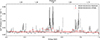 |
Fig. 2. Zoom of the unfolded Resolve and Xtend spectra in the 6.2−7.2 keV band after the continuum modeling, highlighting the presence of strong emission features. The spectra are rebinned visually at a 2σ significance level for illustrative purposes. |
We show the result of the blind search in the left panels in Fig. E.3, with clearly identifiable features for Ca XX, Cr XXIII, Fe I9 Fe XXV, Fe XXVI, and Ni XXVII in resolve. In Xtend, we note a significant emission feature compatible with a Ne X Kα transition. Not only are there no strong edges at this energy, but the feature strongly varies along the observation (see Sect. 3.4), and is clearly detected in the NICER observations of the previous days, thanks to a luminosity an order of magnitude higher. Most importantly, a Ne X Kα feature was already unambiguously detected in one of the Chandra observations of a similar state in a previous outburst (Shaw et al. 2022).
We fit the lines in the Resolve and Xtend spectra, focusing on the emission lines with an individual component at more than 2σ confidence, using the features in the blind search as a starting point. With the limited S/N of the observations, gaussian components were sufficient to describe the line shapes. We fitted the individual components separately whenever possible, and otherwise used a single line when a single line was enough to describe the entire feature, namely for all features below 6.5 keV except for the Cr XXIII He complex, whose w transition can clearly be identified. We present the results of our fitting in Table 2, and show the significance of the lines, first using C-stat. We leave the widths free for all components, except the three that remained unconstrained within the observation; namely, Ne X (due to being only present in Xtend) and Cr XXIII and Ni XXVII (both with a very limited S/N). In all three cases, we froze the line widths at 0 in the analysis. Most lines were previously identified in Shaw et al. (2022) thanks to a much higher luminosity, except for the Cr XXIII complex and Ni XXVII complexes, whose w transitions have EWs significant at a 95% and 97% significance level, respectively. For Fe XXV Kα, we only fit components for the w and y transition, since only these two transitions are seen at a statistically significant level in the blind search. We show the line parameters derived from our fit in Table 2, including the combined velocity correction considering the Earth’s movement in the solar system, the relative velocity of the binary relative to the solar system, and the orbital velocity of the BH within the binary. Details of its computation can be found in Appendix A. In addition, to test the significance of the lines while accounting for the look elsewhere effect and photon noise, it is necessary to perform a set of Monte Carlo (MC) simulations (Porquet et al. 2004). We thus generated 1000 simulated Resolve+Xspectra using the fakeit command in xspec from the best-fit continuum model, retaining all observational parameters of the initial spectra. In each case, we started by refitting the continuum-only model to derive a baseline C-statistic. Then, for each line complex, we added the same component(or components, when the lines are resolved) used to fit the initial dataset, using the width of the best fit for each complex, and tying normalizations between components when relevant. We then scanned the [ − 1000, 1000] km s−1 velocity shift band for C-stat improvements. This band corresponds to the velocity shift range expected in physical systems. We refer to Parra et al. (2024) for an overview of velocity shift signatures before XRISM, and XRISM Collaboration (2025a), Miller et al. (2025b,a) for recent XRISM results for sub and Super-Eddington XRB sources, all with lines within this velocity range. The distribution of the maximum ΔC-stat of the artificial complexes in each spectrum could then be compared to that of the real spectrum. Overall, we define the significance of the real complex as P = 1 − N/1000, with N as the number of simulated spectra where the maximum ΔC-stat achievable for the given complex is higher than the real ΔC-stat value obtained in our observation. All MC significance values are shown in Table 2. Of the features we initially identified and fitted, only two are below 3σ significance with MC simulations. The first is the Cr XXIII line, which we consider a marginal detection, although its ionization range makes it an expected detection when accompanied by other ionized species such as Ca XX for solar abundances (XRISM Collaboration 2025a).
Significant spectral lines identified in the time-averaged Resolved+Xtend spectra.
The second feature is of different nature. We note that fitting the Fe XXVI Kα transition with a single component leaves a clear residual at ∼7.00 keV (which can be seen as an additional peak in Fig. E.3, and as a residual to physical models in Fig. D.2). We expected no strong line at this precise energy and a Fe I Kβ line would require a redshift of ∼3000 km s−1 to reach 7.00 keV. We thus modeled this feature with a second resolved Fe XXVI Kα component, resulting to an improvement of ΔC of 12. This tentative secondary component (which we refer to as the “fast” component in the rest of the analysis, in contrast to the main “slow” component), has a small width, which we constrained to below 3.2 eV at 90% significance. This allowed for very good constraints to be placed on its velocity, derived as −1290 ± 90 km s−1, and below −800 km s−1 at a 3σ confidence level. To assess its significance more precisely, we once again used MC simulations, this time with a velocity shift band of to [ − 3000; 3000] km s−1 around the Fe XXVI Kα line energy, and a resolved Fe XXVI complex. To reproduce this complex, we used two Gaussians at the rest energy of the individual transitions, with tied widths, a Lyα1 normalisation fixed to twice that of Lyα2, and both transitions fixed at a width of 1 eV. Our choice of velocity shifts corresponds to an energy band of [6.90, 7.04] keV and is a conservative estimate of the band where serendipitous, high velocity detections could be associated to the Fe XXVI line, and not other components such as Fe I Kβ or Fe XXV Kα.
With this method, we derived a significance of 99.2% (2.6σ) for this secondary component. While line searches among active galactic nuclei (AGNs), with flux levels comparable to our observation, typically use thresholds of 95−99% for their line detections (Tombesi et al. 2010; Matzeu et al. 2023), the commonly accepted detection threshold for XRBs (albeit suited for objects 1 to 2 orders of magnitude brighter) is of 3σ. We thus only considered this line as a marginal or tentative detection. In addition, we note that this significance was derived for a width of the main Fe XXVI Kα component below ∼20 eV. At widths of ≳20 eV, the main component covers a part of the secondary feature at higher energies, and thus the ΔC of the secondary component is reduced to 8. This parameter space remains however very unlikely, since the corresponding Δv for the main Fe XXVI Kα component would end up ≳3 times higher than that of every other line detected in the spectrum. If the presence of two components can be confirmed with subsequent observations, to the best of our knowledge, it would be the first time a narrow emission component with a blueshift above 1000 km s−1 would be identified in the X-ray band in a BHLMXB. The neutral Fe Kα line, on the other hand, shows an important redshift, albeit with weaker constrains, with a velocity derived at  km s−1 after correction, and above 0 at a > 2σ confidence level.
The rest of the lines show a trend for weak blueshifts, but none are statistically significant. Since their values are all compatible within errors, we tested the effect of linking the blueshift of the 6 components (SXVI, Ca XX, Cr XXIII, Fe XXV, Fe XXVI-slow, and Ni XXVII). This results in a very similar fit (ΔC = +9 for 5 free d.o.f.), and a common velocity of  km s−1 at 90% confidence level after correction, showing weak blueshift trend for these lines, but is insufficient for a physical interpretation. We note that aside from being corroborated by other detections in previous observations (Shaw et al. 2022), the very low velocity shift of these components means that odds of serendipitous detections due to photon noise are much lower compared to the fast Fe XXVI component, for which we purposely scanned a wide range of energies.
Following the fit of these components, we performed a new blind search to assess the significance of the residuals remaining in the spectra, with the results shown in the right panels of Fig. E.3. All lines were correctly fitted and only very weak (and nonsignificant) residuals remained, notably from expected transitions around the Fe XXV Kβ and Fe XXVI Kβ complexes. We do note a duet of puzzling emission features around 6.8 keV, which, while not individually significant at 3σ, match the separation between the (y) and (w) transitions of Fe XXV Kα; thus, it could be a sign of an additional, highly blueshifted (∼ − 5000 km s−1) component. Finally, the emission feature at ∼7.1 keV is unlikely to come from a Fe I Kβ component, as it would require a very high blueshift (∼ − 1800 km s−1) incompatible with the Fe I Kα. Instead, it is more likely to be due to the start of the iron edge at 7.12 keV, which can exhibit a very complicated profile depending on the composition of the absorbing material (Rogantini et al. 2018), which we cannot resolve with our limited S/N.
3.3. Photoionized plasma models
We modeled the photoionized emission lines with the plasma code pion (v3.08.00), implemented within the X-ray spectroscopy analysis software SPEX. We used the default cross-section measurements, namely from the OPEN-ADAS database10. Here, instead of fitting in SPEX, we extracted emission lines calculated by pion and constructed an additive table model (atable) that can be implemented into XSPEC. This makes fitting much faster, as SPEX recalculates the photoionization state self-consistently with every iteration of the continuum. To address this issue, we fixed an illumination SED shape and precomputed the photoionization states and spectra, compiling them into a table model.
We calculated a grid of models for solar abundances, simulating emission with different values of column density NH, ionization parameter log ξ, and turbulent velocity vrms. This simulation includes free-free emission, line emission, and recombination lines. Each of the simulations has 65536 logarithmically spaced bins to cover the energy range from 10−4 to 103 keV with a resolution of 1.5 eV around 6 keV, enough to fit Resolve data. In total, we perform 8736 simulations with values 21 ≤ log NH ≤ 25 spaced by 0.2 (21 points), 2 ≤ ξ ≤ 7 spaced by 0.2 (26 points), and −5 ≤ log(vrms/c)≤ − 2 spaced by 0.2 (16 grid points). We assumed a single number density np = 1012 cm−3 to reduce the size of the tables. We calculated the population levels from radiative recombination, cascade, radiative, and collisional excitation correctly for metastable levels.
Adding this photo-ionized emission to the continuum gives a good fit to the data (see Table 3), and successfully matches all the emission lines in the data (see Fig. 3), except for the 6.4 keV Fe Kα fluorescence line and the secondary Fe XXVI component, which are expected to arise from different material considering their distinct velocity shifts. The ionization state is well constrained at log ξ = 3.9 ± 0.1, but the column density is not, as this mostly sets the overall normalization. In addition, the velocity, after adding the correction of −117 ± 13 km s−1, is derived as −240 ± 70 km s−1, which is not only two times the common blueshift value derived from line fitting in the previous section, but also more significant by 3σ. The difference with our empirical fitting is likely due to a more physically consistent fitting of the line shapes, along with the addition of the main higher complexes of the iron lines. We note that the uncertainty in the systematics, unlike that of the fit, is a fixed value. Once again, we confirm the presence of residuals with a blind search in the entire Resolve band. The results for the iron band are shown in Fig. D.2, and the rest of the spectrum in Appendix E.
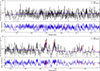 |
Fig. 3. Residuals of the Resolve unfolded time-averaged spectra with the model of photo-ionized plasma emission (red) and the numerical MC radiative transfer simulation (blue). These two models are fitted simultaneously to the Xtend and Resolve data, with the Xtend data omitted from the plot for clarity. |
Best-fit parameters of the photoionized plasma model.
3.4. Time-resolved analysis
V4641 Sgr is known for its dramatic spectral evolution on very short timescales (Hjellming et al. 2000). When computing the light curve of the source in several bands, as shown in the left panels of Fig. 4, we see that although the higher energies remain relatively stable, at lower energies, the source brightens by a factor ∼3 between the beginning and the end of the observation. To investigate the changes in continuum and line properties, we thus derive Resolve and Xtend spectra for each of the individual orbits, which we show in the right panels of Fig. 4. We further divide the last orbit into two periods due to its strong evolution in flux, and refer to the two as different orbits due to the small observing gap between them. Despite a very limited S/N, the source shows both a strong continuum evolution at low energy and changes in line properties.
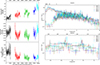 |
Fig. 4. Left: Xtend light curve and HR of the observation with bins of 128 s, highlighting the different orbits used for time-resolved spectroscopy. Right: Folded Xtend and Resolve spectra of individual orbits of the observation (top) and zoom of Resolve to the 6.3−7.3 keV band (bottom) rebinned for visual clarity. |
We first assess the evolution of the continuum by fitting the Resolve and Xtend spectra of each orbit together, while ignoring all the energy bands where lines were detected in the time-averaged spectrum. Although this progressive variation at low energy is characteristic of a change in the intrinsic absorber obscuring the source, we first attempted to fit each orbit with an independent diskbb and a common ISM absorption component. The resulting fit, although globally satisfactory (C-stat/d.o.f. ∼ 1.2 in Xtend), is much worse for the first three orbits, and results in completely unphysical disk parameters, with notably an inner temperature in the first orbit of  keV. We thus fitted all orbits together with a second model including a partial covering absorber, modeled with cabs*pcfabs within Xspec, whose column density and covering fraction can vary between orbits within the limits described below, and a disk that remained constant along the observation. To consider the influence of Compton Scattering in the partial covering absorber properly, as cabs doesn’t include a covering fraction parameter, we defined our model in xspec as TBabs(constant*diskbb+cabs*pcfabs*constant* diskbb), where each disk represents the uncovered and covered fractions. We thus link the parameters of both diskbb, fix the covering fraction in pcfabs to 1 (this represents the fully absorbed component), and fix the value of the second constant to 1 – the first constant, so as to act as a covering fraction parameter. Finally, we link the absorption of the cabs component to that of the pcfabs. To limit the degeneracy between the absorption components and the disk normalization, we fix the covering fraction in the brightest orbit at 0, and the ISM column density at NH = 0.15 × 1022 cm−2. With this choice, we focus on constraining the additional absorber between the last and first orbit. We stress that constraining the entirety of the intrinsic absorber with soft X-ray data alone is not possible: a fully ionized component would only be seen via Compton Scattering and thus a cross-section that is almost constant along the entire XRISM bandpass. This means that the column density of that component is completely degenerate with the normalization of the disk component. Meanwhile, an additional partially ionized absorber present in all observations would be degenerate with both the disk normalization and temperature. We can only constrain the lack of a fully cold, nonionized zone, similarly to other objects such as GRS 1915+105 (Miller et al. 2025a). Since Resolve and Xtend were perfectly matched in the time-averaged spectrum, we do not use a constant factor between the two instruments.
We show the parameters of the fit in Table 4. The quality of the fit is similar to the empirical fit with varying disk parameters, while retaining physical consistency. We measure an increase of 50% in flux between the first and last orbits, and a diminution of ∼40% of the 3−10/1−3 keV hardness ratio. However, in part due to our limited statistics, the fit remains very limited, as despite a progressive decrease in covering fraction between orbits, orbits 2 to 4 barely constrain the column density of the absorber. Moreover, the Xtend statistics of the first three orbits remain significantly higher than the last two orbits, hinting at a much more nuanced absorber structure than what our simple model can constrain. In hope of reaching a better agreement between the first and last orbits, we tested several different variations of the model, such as thawing the ISM column density, using a variable ionized partial covering (with zxipcf), and a physical comptonized disk model (thcomp(kerrbb)) inside the partial covering. None led to a meaningful improvement in the fit.
Best-fit continuum parameters for the individual orbits using a partially covered disk model.
In parallel, we can see the iron lines vary in both energy and strength in the zoomed iron spectrum shown in the bottom panel of Fig. 4 (we stress that these spectra are visually rebinned but retain a much higher resolution). This hints at a much more complex evolution in the absorber obscuring the source than what can be assessed with continuum fitting, but the S/N of each line remains very marginal with only ∼2 − 2.5 ks of exposure per orbit. We thus limit ourselves to the lines detected in at least one individual orbit. Once again, to help visual identification of significant residuals, we start by performing a blind search for narrow features in each observation period, of which we show a summary in Fig. E.1. We then fit lines in each orbit based on lines previously identified in the time-averaged spectrum, complemented by the results of the blind search. We restrict ourselves to the lines with a 99% significant ΔC after fitting in at least one of the five orbits. All orbit-resolved line parameters are presented in Table D.1. We note that the majority of the lines were already identified as significant in the time-averaged spectrum. The two exceptions are the Fe Fe XXV Lyβ and Cr XXIII Hew transitions, for which we performed MC simulations in the respective orbits in which they are detected. Thanks to the very low photon noise of XRISM for narrow lines, both are identified above a 3σ (99.7%) significance level.
Despite a very limited S/N, we can thus confirm the trends seen visually in the spectrum, with a remarkable amount of variability in several different complexes, in part unrelated to changes in the continuum absorber. First, our fits show a surprising switch from an intercombination-dominated Fe XXV He profile in the first four orbits, to a resonance-combination dominated profile in the final orbit. In addition, although we detect a rise in the EW of the strongest component along the orbits, the significance is too low for any definitive conclusion. Meanwhile, the Fe XXVI Lyα profile, aside from a strong but marginally significant increase in EW in orbit 2, shows a remarkable velocity evolution, from being compatible with zero in the first four orbits, to being very significantly redshifted in the last observation, at  km s−1 after orbital corrections. This value is at odds with the well-constrained, almost static (
 km s−1) Fe XXVI Kα line seen in the same orbit, and thus the two lines must originate from two distinct absorbers, at least in this orbit. Finally, although this may be spurious, we note that this redshift matches that of the weak Fe I Kα feature detected in the time-averaged spectrum. In the weaker lines, the Cr XXIII Hew transition is only detected in a single orbit, with a very high EW, and ends up diluted in the time-averaged spectrum. On the other hand, the Fe XXV Lyβ line, which was not significant in the time-averaged spectrum, is only detectable in orbit 2, but unlike the Cr transition, the respective lack of detection in other orbits is not significant enough to conclude on its evolution in the rest of the observation. Finally, although the evolution of the Ne X Lyα is difficult to disentangle from that of the poorly fitted continuum at low energies, there is a progressive change from a complete lack of line in the first orbit, to a very strong and significant feature in orbit 5.
4. Optical analysis
In this section, we focus on the optical Seimei spectra simultaneous to the first half of the XRISM observation and whose data reduction procedure is detailed in Sect. 2.3. In Fig. 5, we show the overall spectra of the two grisms. The H Balmer lines (Hα and Hβ), He lines, and Fe II line are detected in absorption, as normally seen from the intermediate mass companion star (B9III: Muñoz-Darias et al. 2018), but the Hα profile shows an additional emission component. Although we can derive widths and velocities of the order of ∼100 km s−1, the limited spectral resolution of the Seimei telescope is insufficient to properly characterize these spectral components and disentangle the contribution of the donor star quantitatively. However, we can still compare the BH and donor spectrum qualitatively. For this, we perform empirical fitting of the components, both for our spectrum and the averaged donor spectrum obtained by Muñoz-Darias et al. (2018) in October of 1999 during quiescence, in which the contribution of the accretion disk and the disk wind is expected to be negligible. We show the resulting comparison for the main lines of interest in Fig. 6. Although the Hβ line profiles are broadly consistent between the two spectra, the Hα line profiles are different, with a clear additional emission component in the BH spectrum. In addition, several additional lines, notably from HeI and Fe II, are seen in the Seimei spectrum in panel c, and may include a component intrinsic to the BH, but the majority are also seen in the donor spectrum in panel f, albeit with weaker normalization. The only exception is a very weak He I-6678 seen in panel e, with a negligible velocity shift, and no counterpart in the donor spectrum. The different Hα profile could be due to an accretion disk atmosphere, or a disk wind with marginal velocities of a few ∼100 km s−1, to match the measurements considering the systematics of the Seimei observation. In addition, the Seimei observations were performed as ten 10-minute segments for VPH 683, and 3 5-minute segments for VPH 495, both covering the first half of the XRISM observation. In light of the highly variable line features seen in X-ray, and considering the fast variability seen in recent OIR spectroscopy results (Miceli et al. 2024), we also extracted the spectra of both grisms for each individual snapshot. Although we detect some variability in the profile of the Hα component, the limited S/N and strong evolution in atmospheric transmission along the observation prevent any interpretation.
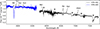 |
Fig. 5. Optical spectrum obtained with the Seimei telescope. The blue and black data show the spectra obtained with the VPH-495 and VPH-683 grisms, respectively. Finally, ⊕ indicates the atmospheric lines. |
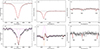 |
Fig. 6. Most relevant spectral lines in the donor (top) and Seimei (bottom) spectra and empirical best-fit models. In the Seimei spectra, the contributions of the individual components are indicated by dashed lines. |
5. Discussion
5.1. Continuum and global spectral evolution
Although the intrinsic luminosity and SED of the source are very difficult to constrain directly, we can still draw parallels to standard outburst patterns. The most obvious similarity is the apparent state change during the second part of the outburst: as seen in the lowest panels of Fig. 1, and according to the spectra analyzed in Sect. 2.2, this long-term evolution is reminiscent of a standard soft-hard transition at ∼10−2 Eddington (see, e.g., Vahdat Motlagh et al. 2019; Wang et al. 2023), obscured by a factor 10 by a steady, fully ionized absorber. Meanwhile, a second, highly variable layer would be responsible for the erratic dips and HR evolution during the transition, be it due to outflows or an inhomogeneous geometry. We highlight this scenario in Fig. B.1, with the proposed distinction between the steady evolution (one absorber) and the more variable dips signaling an additional absorber. These dipping periods are typically harder, hinting at a partially ionized layer that would have a stronger absorption at low energies, and would be compatible with the NICER and Swift spectra at first order. The evolution of this layer could be what is seen in our time-resolved analysis in Sect. 3.4, and correspond to the main absorbing layer seen with the XRISM emission lines. The evolution of the lines as seen in NICER, and notably the lack of lines in most of the non-dip spectra, could then be directly due to that of the partially ionized layer, but a quantitative description is limited by the weak NICER S/N at these flux levels and requires a separate analysis.
However, this scenario remains insufficient to describe the entire outburst evolution. First, assuming that the steady absorber also dominated the long-term behavior of the source for the first weeks of the outburst, a standard outburst pattern would also include a noticeably brighter period (typically by one order of magnitude), matching the bright hard state, hard-to-soft transition, and bright soft state. However, the soft state plateau at 10−3 LEdd (seen at the beginning of September and preceding the decay) seems to be the peak of the outburst luminosity, as seen in the EP and MAXI monitoring light curves with a longer coverage. This is also compatible with the soft state spectra seen across several weeks in the previous outburst (Shaw et al. 2022), although they showed significantly lower disk temperature. Secondly, the multi-wavelength behavior during the state transition hints at a much more complex evolution than a simple varying absorber. While the first (very weak, 0.17 mJy) radio detection, and subsequent nondetection (< 87 μJy) at the start of the transition (Grollimund et al. 2024b), are compatible with a low-luminosity soft state, the detection matching the very end of the transition (Grollimund et al. 2024a) is at odds with our scenario. First, its low spectral index (α = −0.4, Source: N. Grollimund, priv. comm.) is at the edge of the delimitation between transient ejecta and compact jet. Secondly, that detection (15.5 mJy) is not only 200 times brighter than the transition upper limit, but its absolute value itself remains uncharacteristically bright relative to the unabsorbed X-ray luminosity for a soft-to-hard transition, and would thus point toward high obscuration levels.
Indeed, while it is difficult to draw conclusions on radio detections at such a low α, the X-ray luminosity does not decrease significantly during the soft-to-hard transitions, and the radio luminosity can thus be used to retrieve a lower limit of the X-ray luminosity of the previous soft states, (see, e.g., Fig. 3 in Hughes et al. 2025a for a recent study with extensive radio outburst coverage). Thus, if this radio detection is from a standard compact jet, we use this detection to derive an approximate lower limit of the X-ray Eddington ratio during the soft state preceding the transition, which we expect to be less obscured. Our radio detection translates to LR − 5GHz = 3.4 × 1030 erg s−1 for a a distance of 6.2 kpc. To match the slope of the Radio/X-ray correlation (see Hannikainen et al. 1998; Corbel et al. 2003; Gallo et al. 2003; Corbel et al. 2013; Hughes et al. 2025b for a more recent overview), we derive that even a radio bright source would require LX ≳ 5 ⋅ 1037 erg/s, or LX ≳ 6 × 10⁻² LEdd, which would be at least an order of magnitude above our assumed Eddington ratio during the same period. If this extrapolation is valid, it would imply that the source is more obscured, with a soft to hard state transition starting at LX ≳ 10−1 LEdd instead of the expected LX ∼ 10−2 LEdd. The previous radio measurements at very low level do not provide significant information: residual core radio emission can sometimes be seen at significant levels during the soft state (Hughes et al. 2025b), but this is only true for some objects, and correlations with X-rays and physical parameters have yet to be properly quantified. The other (simpler) possibility is that this event signals a more complicated accretion-ejection reconfiguration that doesn’t fit the standard radio outburst evolution, nor the Radio X-ray correlation. This could explain the very important X-ray luminosity and hardness-ratio evolution just before and after that event, if, for instance, this event is linked to an ejection of some of the obscuring layer. Available radio observations thus do not allow to directly distinguish a high and low Eddington ratio interpretation.
Finally, we highlight that the neutral column density derived in our analysis is significantly lower than that used in Shaw et al. (2022), who fixed theirs to 2.5 × 1021 cm−2, following a previous Swift-NuSTAR fitting (Pahari et al. 2015). Our own analysis of Swift and NICER spectra of this outburst (see Sect. 2.2) required an additional absorber of up to 3 × 1021 cm−2 to match the continuum below ∼2 keV, most notably at higher luminosities. We stress that without a good understanding of the intrinsic absorber, all values of NH remains highly degenerate, and the estimate in our analysis is still likely to be higher than the ISM absorption, which, in the direction of the source, only amounts to ∼1.6 × 1021 cm−2 when integrated over the entire galaxy (HI4PI Collaboration 2016), and should thus be significantly lower for a source only at 6.4 kpc.
5.2. physical interpretation of the X-ray line emitters
In the X-ray spectrum, several narrow emission lines were successfully detected, despite the short exposure of ∼10 ks and the low source intensity of ∼1 mCrab. All of these, except for the Fe I Kα and the secondary blueshifted Fe XXVI Kα component, are well modeled by emission from a single layer of photoionized material above the disk. This model and the ion-by-ion line fitting show a significant blueshift, meaning that this X-ray line emission is likely to come from a disk wind. We can estimate the radius of the material by assuming that the velocity width comes from the Keplerian velocity around the launching radius, since the high-density, line-emitting gas is expected to be close to the disk surface. This gives that R/Rg = 0.5(c sin i/vrms)2 = (8 ± 4)×105, where i = 72 ± 4° is the inclination angle of this source (MacDonald et al. 2014). The outer disk radius should be at 70% of the Roche-lobe radius, giving Rout/Rg = 6 × 10⁵. Thus, the estimated radius is at the outer edge of the disk.
The fit parameters also enable a tentative estimate of the intrinsic luminosity L0. The wind material is directly irradiated, so its ionization parameter is set by ξ = L0/(nR2). With the column density as NH = nΔR ≈ nR, we derive  erg s−1. This is about 104 times higher than observed, and implies that the source may be intrinsically super-Eddington, with
 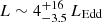 . This extrapolation is very dependent on the estimate of the launching radius, but would also match the observed high temperature of the disk blackbody continuum. While it is quite surprising that the wind is so slow at such super-Eddington fluxes, and that the scattered fraction is so small, we note that this is somewhat similar to the wind parameters inferred in the neutron star super-Eddington source GX 13+1 (XRISM Collaboration 2025a).
As a qualitative comparison to a more physical wind launching model, we compared this observation to a single simulation of scattering from a thermal wind (blue in Fig. 3). This simulation was tailored for the neutron star binary system GX 13+1, with a Compton temperature of 1.3 × 10⁷ K, corresponding to a DISKBB component of 2.3 keV (Tomaru et al. 2023, 2020). This is a little hotter but still comparable to that seen here. The intrinsic luminosity was set to L/LEdd, NS = 0.5, or 8.8 × 1037 erg s−1, and would translate to L/LEdd, BH = 0.11 for our source. As seen in Fig. 3, this model gives a fairly good overall description of the photoionized emission, showing that emission from a thermal-radiative disk wind can explain the main ionized scattering layer. However, this model does not include obscuration, and we would thus require an additional, fully ionized absorber to obscure the spectrum by a factor 1000, down to the observed luminosity of L/LEdd, BH = 1.45 × 10⁻⁴. With pure Compton scattering, we can estimate this would require an additional column density of NH ∼ 8.5 × 1024 cm−2.
In parallel, the origin of the secondary components remains puzzling. The redshifted Fe I Kα line, whose velocity is barely compatible with the main component at a 3σ confidence level, can be produced where X-rays illuminate mostly neutral material. Potential sites include the accretion disk itself, but the inner disk is highly ionized, and the outer disk should be covered by the highly ionized wind. The outer disk surface under the wind (below the thermal instability) could also produce lines, but they would likely still be mildly ionized and give an apparent blueshift rather than a redshift. Meanwhile, the tentative fast blueshifted component, being detected in Fe XXVI only and not in Fe XXV, points toward a very high ξ and thus an entirely different emitting region, closer to the central region than the main obscuring layer (important for, e.g., radiation pressure to accelerate it to ∼ − 1300 km s−1).
Within the context of the recent discoveries of systematically clumpy outflows from highly accreting AGNs, not only for ultra-fast outflows but also for warm absorbers (see, e.g., XRISM Collaboration 2025b; Xu et al. 2025; Mehdipour et al. 2025; Xiang et al. 2025), it can be tempting to adapt this scenario to V4641 Sgr. Although this could explain very well both the fast variability and diversity in absorbers, ionization parameters, and velocity shifts, the mix of redshifted and blueshifted components remains puzzling. One possibility would be for the Fe I Kα line to originate in an outflowing material in the backside of the accretion disk, while the frontside would be suppressed by one of the main absorbing layers. This, however, cannot explain the switch to a purely redshifted Fe XXVI Kα line in one of the orbits. Another possibility would be that clumps of material from a “failed” wind progressing toward the BH occasionally cross our line of sight. As different components may evolve on different timescales, and we lack an adequate S/N to distinguish meaningful changes in the Fe Kα line in single orbits, this emission could be created by a similar scenario. Future observations, especially during brighter states, will allow us to distinguish transient in-falling absorbers from a more steady backside outflow.
Finally, a comparison to the results of the photoionized computation derived in Shaw et al. (2022) is not straightforward, due to the differences in illuminating SEDs, photoionization codes, and methodology. In the future, analyzing all spectra using the same approach will help assess how much the main ionized layer at the origin of the emission lines evolved between the previous and current outburst. Moreover, the Chandra observations, with their higher luminosity, have sufficient S/N to perform time-resolved spectroscopy and search for the high diversity of line variability found in our observation, at least qualitatively, something which was not investigated in previous works.
5.3. Contextualization of the optical emission
Although quantitative measurements are limited by the high contamination by the companion star, the simultaneous optical data offers a complementary view, with an Hα emission line with negligible redshift yet low enough ionization parameter to match the Fe I Kα emission. This Hα emission is likely formed in a dense, clumpy optical wind (Muñoz-Darias et al. 2018), but we note very significant differences compared to the more active spectra in the previous outbursts, with a lack of significant blueshifted P-Cygni profiles or blue wings in Hα and Hβ, or significant He-5876 absorption. This is the aspect most at odds with a highly accreting and outflowing scenario: in all outbursts previously observed and studied in Muñoz-Darias et al. (2018), the optical magnitudes drop extremely rapidly after the initial bright events, and strong wind signatures can be seen up to several weeks after the outburst peak. We do note, however, that the wind signatures become much weaker in some observations, with the Hα emission line being the most clear remaining component, and could then be compatible with what is seen at lower S/N in the Seimei spectrum. In 2024, no increase of optical magnitudes above ∼0.5 was detected (Goranskij et al. 2024). However, we note that the optical monitoring was limited around the approximate peak of the X-ray outburst, with a notable observing gap between September 4 and September 14 (V. Goranskij, priv. comm.).
Several possibilities can thus explain the lack of strong wind signatures in our optical spectrum. The most straightforward result is that the optical monitoring serendipitously coincided with a less pronounced wind phase, but this remains at odds with the high diversity of absorbers seen in X-rays and their variability, which indicates actively evolving and outflowing phases. Another is that this outburst truly never reached the high Eddington ratios of ≳0.1 LEdd, which preceded the presence of the strong optical wind signatures in previous outbursts. However, many other BHXRBs have shown strong OIR wind signatures down to very low Eddington ratios (e.g., ∼10−4 LEdd in Sanchez-Sierras & Munoz-Darias 2020). Finally, the obscured soft state X-ray SED may signal an accretion configuration which, despite its expected very high intrinsic luminosity and peculiar geometry, suppresses optical wind signatures independently of the state of the outflow, similarly to what is seen in standard outbursting BH LMXBs soft states (Mata Sánchez et al. 2022), or even suppresses the cold outflows completely. This would strongly contrast with the spectra discussed in Muñoz-Darias et al. (2018), which were typically simultaneous to hard X-ray SEDs.
Confirming that this recent (also seen in e.g., Shaw et al. 2022) soft obscured state coincides with an invisible, more ionized, or completely absent cold wind phase will require denser multi-wavelength monitoring during future outbursts. Still, as long as this source remains the only obscured BHXRB with both soft and hard X-spectral states, it will remain one of the best candidates to study the link between the illuminating X-ray SED, highly ionized absorbers, and the presence (or detection) of optical wind signatures. Although this link is already largely suspected, as the hot wind phase is detected in X-rays in typical soft states (Ponti et al. 2012; Parra et al. 2024), and the cold wind phase can be seen in infrared along the entire outburst (Sanchez-Sierras & Munoz-Darias 2020), we currently lack in depth studies modeling the effect of soft X-ray SEDs on the presence of OIR wind signatures. In parallel, a more exhaustive study of the correlation between X-ray SED and OIR wind signatures (which has yet to be done for this source) could reveal whether the configuration of 2024 is an outlier or the standard behavior for such atypical outbursts.
6. Conclusion
V4641 Sgr is a unique BHXRB, whose X-ray spectra show an obscured central engine and narrow emission lines (instead of absorption lines) from a disk wind. Although similar features were observed in V404 Cyg and GRS 1915+105, these sources showed both hard spectra and extreme flux variability when obscured. In contrast, V4641 Sgr often shows a soft thermal spectrum and can exhibit a stable flux over several weeks.
In this study, we present the results of our high-resolution multi-wavelength monitoring campaign of V4641 Sgr during the 2024 outburst. Our 10 ks XRISM spectrum, taken during an obscured dip at 1 mCrab at the end of a transition to an obscured hard state, reveals a soft, thermal-like spectrum dominated by a high temperature thermal disk component of 1.77 ± 0.03 keV (or  keV with a comptonized disk). The Resolve and Xtend spectra show many strong, narrow emission lines. Most of them come with marginal blueshifts, which can be well represented by a single ionized (log ξ = 3.9) photoionization layer in emission with a very high column density (
 cm−2) and a small but significant blueshift of −240 ± 70 km s−1 after corrections. The very low Eddington fraction of the observation (∼1.5 × 10⁻⁴) and the high disk temperature strongly hint at an additional, strongly ionized (and thus largely unconstrained) obscuring layer, that would absorb the spectrum by at least one order of magnitude.
We detected signs of two additional layers in the spectrum: the narrow, redshifted Fe Kα line ( km s−1) indicates an infalling clump with low ionization or scattering from an outflow in the back of the disk, and a marginally significant (99.2% with MC simulations) strongly blueshifted secondary Fe XXVI Kα emission component (−1290 ± 90 km s−1) may be caused by a weaker inner wind component at high ionization. Moreover, the time-resolved spectrum shows a rapidly changing continuum, which softens by a factor of two and becomes 50% brighter in the 10 ks of observation. The latter is accompanied by significant changes in the line properties and the ratios of individual transitions between the individual orbits. Although the weak S/N limits the analysis for such small exposures, the most remarkable changes are a very significant switch from a slight blueshift for the Fe XXVI Kα line to a strong redshift (
 km s−1) in the last orbit, requiring an additional component compared to the well constrained, static Fe XXV seen in the same segment. Finally, we see a clear switch from an intercombination-dominated Fe XXV Kα complex in the first orbits to a resonance-dominated line in the last.
Although the optical Seimei spectrum is strongly dominated by the companion star and associated absorption features, a clear additional emission component is evident in Hα. This single detection starkly contrasts with the very strong P-Cygni and blueshifted asymmetric emission and absorption line profiles often observed in this source following the brightest portion of previous outbursts (Muñoz-Darias et al. 2018).
While the picture provided by these datasets is still incomplete, the context of the available X-ray monitoring shows that this observation was made at the end of the transition from a faint, weakly variable soft state (which might have marked the peak of luminosity of the outburst) to a pure, decaying hard state (which later dimmed down to near-quiescent levels). As the entire outburst is likely obscured by at least an order of magnitude, this transition might be comparable to a soft-hard transition in normal outbursts. In that case, the correlation between the X-ray evolution and the radio measurements, which show an increase of more than two orders of magnitude between the start(< 87 μJy) and end (15 mJy) of the state transition, suggests a second, more variable absorbing layer that may have been partially ejected during the radio flare.
Meanwhile, a simple extrapolation from the absorber parameters, as well as comparisons with physical, radiation-driven wind models tailored to the near-Eddington source GX 13+1, show that the obscuration of the main ionized line-emitting layer of this source is consistent with a near- or Super-Eddington intrinsic luminosity. However, this scenario would require an extreme obscuration of three to four orders of magnitude.
This observing campaign perfectly demonstrates the power of XRISM Target of Opportunity observations, even with low exposures. Thanks to the exquisite spectral resolution of Resolve, the instrument can reveal entirely new information about the X-ray features in accreting sources, investigating line variability on new timescales; furthermore, small observing campaigns can serve as a probe to assess the scientific potential of longer observations. In our case, realistic future observations of V4641 Sgr in a less extremely obscured state (e.g., 20 mCrab) and with higher exposure times (i.e., 100 ks) would allow for an order of magnitude improvement in the constraints placed on all line complexes. Aside from a definitive answer on the existence of the fast wind component and more precise measurements of the velocities of the redshifted Kα line and the weakly blueshifted main component, new observations would certainly enable the identification of many additional transitions and secondary components that we have not discussed here due to their weak significance. In parallel, it would be possible to constrain the evolution of these strong lines and absorbers down to timescales of one minute and along an entire orbital period, which would open new opportunities to understand the influence of the (high-mass) companion on the absorber dynamics. A higher S/N would also enable more advanced line diagnostics for several line complexes (Porquet & Dubau 2000) and, notably, for Fe XXV Kα (Shaw et al. 2022). However, these results should be computed carefully due to degeneracy between several effects, among which continuum pumping (Chakraborty et al. 2021), resonant Auger Destruction (Chakraborty et al. 2020), and resonant scattering, which require detections of higher-order complexes to be disentangled (Mewe et al. 2001). We also note the direct effects of high optical depths on low-ionization lines such as Ne X (Chakraborty et al. 2022) that could be quantifiable with a higher S/N; most notably with the Gate Valve in its open configuration.
For now, a more comprehensive view of the global evolution of this outburst, using the extensive simultaneous coverage of the INTEGRAL observatory, would provide much stronger constraints on the presence and evolution of the comptonized component, as well as the XMM-Newton/RGS observation performed earlier in the outburst, could shed more light on the nature and evolution of low-ionization absorbers. Finally, a more holistic study of the NICER coverage of this source during recent outbursts and comparisons with the existing radio monitoring will be critical to relating its outburst evolution to that of standard sources and extrapolating its intrinsic Eddington ratio.
Data availability
Appendix E, which includes the full results of the blind searches for the time-averaged and time-resolved spectra, is available on Zenodo at https://doi.org/10.5281/zenodo.19382127.
Acknowledgments
We thank the XRISM operation team for accepting our DDT proposal and conducting the observation. This research has made use of software provided by the High Energy Astrophysics Science Archive Research Center (HEASARC), which is a service of the Astrophysics Science Division at NASA/GSFC. The Seimei telescope at Okayama Observatory is jointly operated by Kyoto University and the National Astronomical Observatory of Japan (NAOJ), with assistance provided by the Optical and Infrared Synergetic Telescopes for Education and Research (OISTER) program. This study makes use of the Seimei data obtained through the program 24B-N-CT03 in the open use of the observing time provided by NAOJ. Part of this work was financially supported by Grants-in-Aid for Scientific Research 19K14762, 23K03459, 24H01812 (MS) from the Ministry of Education, Culture, Sports, Science and Technology (MEXT) of Japan. MP acknowledges support from the JSPS Postdoctoral Fellowship for Research in Japan, grant number P24712, as well as the JSPS Grants-in-Aid for Scientific Research-KAKENHI, grant number J24KF0244. T.M.-D. acknowledges support by the Spanish Agencia estatal de investigación via PID2021-124879NB-I00. EdF gratefully acknowledges support from the Inter-University Research Programme (Grant2025i–F–05) and the Joint Research Program (international) of the Institute for Cosmic Ray Research (ICRR) at the University of Tokyo. He also thanks Marco Pérez from the Centro Universitario de Ciencias Exactas e Ingenierías (CUCEI), Universidad de Guadalajara (UdeG), the Coordinacion de Personal and the corresponding administrative offices of the UdG, as well as the administrative and scientific staff of the ICRR for the financial and logistical support during his invited research stays at the ICRR in 2025. M.A.P. acknowledges support through the Ramón y Cajal grant RYC2022-035388-I, funded by MCIU/AEI/10.13039/501100011033 and FSE+ YZ acknowledges support from the Dutch Research Council (NWO) Rubicon Fellowship, file no. 019.231EN.021. Facilities: XRISM, Seimei: 3.8m, NICER, Swift, Einstein Probe, INTEGRAL, MeerKAT. This work was supported by JSPS Core-to-Core Program (grant number: JPJSCCA20220002). Software: XSPEC (Arnaud 1996), IRAF (Tody 1986).
References
- Alfaro, R., Alvarez, C., Arteaga-Velázquez, J. C., et al. 2024, Nature, 634, 557 [Google Scholar]
- Arnaud, K. A. 1996, ASP Conf. Ser., 101, 17 [Google Scholar]
- Bahramian, A., & Degenaar, N. 2023, Handbook of X-ray and Gamma-ray Astrophysics (Singapore: Springer Nature), 1 [Google Scholar]
- Bahramian, A., Altamirano, D., Heinke, C., et al. 2015, ATel, 7904, 1 [Google Scholar]
- Bianchi, S., Ponti, G., Muñoz-Darias, T., & Petrucci, P.-O. 2017, MNRAS, 472, 2454 [Google Scholar]
- Cao, Z., Aharonian, F., Bai, Y. X., et al. 2025, Natl. Sci. Rev., 12, nwaf496 [Google Scholar]
- Chakraborty, P., Ferland, G. J., Chatzikos, M., Guzmán, F., & Su, Y. 2020, ApJ, 901, 68 [Google Scholar]
- Chakraborty, P., Ferland, G. J., Chatzikos, M., Guzmán, F., & Su, Y. 2021, ApJ, 912, 26 [NASA ADS] [CrossRef] [Google Scholar]
- Chakraborty, P., Ferland, G., Chatzikos, M., et al. 2022, ApJ, 935, 70 [NASA ADS] [CrossRef] [Google Scholar]
- Chakravorty, S., Lee, J. C., & Neilsen, J. 2013, MNRAS, 436, 560 [Google Scholar]
- Charles, P. A., Shahbaz, T., & Geballe, T. 1999, International Astronomical Union Circular, 7267, 2 [Google Scholar]
- Chaty, S., Charles, P. A., Martí, J., et al. 2003, MNRAS, 343, 169 [NASA ADS] [CrossRef] [Google Scholar]
- Cheng, H., Zhang, C., Ling, Z., et al. 2025, Exp. Astron., 60, 15 [Google Scholar]
- Corbel, S., Nowak, M. A., Fender, R. P., Tzioumis, A. K., & Markoff, S. 2003, A&A, 400, 1007 [NASA ADS] [CrossRef] [EDP Sciences] [Google Scholar]
- Corbel, S., Coriat, M., Brocksopp, C., et al. 2013, MNRAS, 428, 2500 [Google Scholar]
- Done, C., Gierliński, M., & Kubota, A. 2007, A&ARv, 15, 1 [Google Scholar]
- Dubus, G., Done, C., Tetarenko, B. E., & Hameury, J.-M. 2019, A&A, 632, A40 [NASA ADS] [CrossRef] [EDP Sciences] [Google Scholar]
- Dunn, R. J., Fender, R. P., Körding, E. G., Belloni, T., & Cabanac, C. 2010, MNRAS, 403, 61 [Google Scholar]
- Eckart, M. E., Brown, G. V., Chiao, M. P., et al. 2024, Proc. SPIE, 13093, 510 [Google Scholar]
- Fender, R. 2003, ArXiv e-prints [arXiv:astro-ph/0303339] [Google Scholar]
- Fornasini, F., Antoniou, V., & Dubus, G. 2024, Handbook of X-ray and Gamma-ray Astrophysics (Singapore: Springer), 3719 [Google Scholar]
- Gallo, E., Fender, R. P., & Pooley, G. G. 2003, MNRAS, 344, 60 [Google Scholar]
- Gatuzz, E., Díaz Trigo, M., Miller-Jones, J. C. A., & Migliari, S. 2019, MNRAS, 482, 2597 [Google Scholar]
- Gendreau, K. C., Arzoumanian, Z., Adkins, P. W., et al. 2016, Proc. SPIE, 9905, 99051H [NASA ADS] [CrossRef] [Google Scholar]
- Goranskij, V. P., Barsukova, E. A., & Fatkhullin, T. A. 2024, ATel, 16916, 1 [Google Scholar]
- Grollimund, N., Corbel, S., & Fender, R. 2024a, ATel, 16852, 1 [Google Scholar]
- Grollimund, N., Corbel, S., Fender, R., & Motta, S. 2024b, ATel, 16819, 1 [Google Scholar]
- Hannikainen, D. C., Hunstead, R. W., Campbell-Wilson, D., & Sood, R. K. 1998, A&A, 337, 460 [NASA ADS] [Google Scholar]
- HI4PI Collaboration (Ben Bekhti, N., et al.) 2016, A&A, 594, A116 [NASA ADS] [CrossRef] [EDP Sciences] [Google Scholar]
- Hjellming, R. M., Rupen, M. P., Hunstead, R. W., et al. 2000, ApJ, 544, 977 [Google Scholar]
- Hughes, A. K., Carotenuto, F., Russell, T. D., et al. 2025a, ApJ, 988, 109 [Google Scholar]
- Hughes, A. K., Carotenuto, F., Russell, T. D., et al. 2025b, MNRAS, 542, 1803 [Google Scholar]
- Ingram, A. R., & Motta, S. E. 2019, New Astron. Rev., 85, 101524 [Google Scholar]
- Ishisaki, Y., Kelley, R., Awaki, H., et al. 2022, Proc. SPIE, 12181, 121811S [Google Scholar]
- Jiménez-Ibarra, F., Muñoz-Darias, T., Casares, J., Padilla, M. A., & Corral-Santana, J. M. 2019, MNRAS, 489, 3420 [CrossRef] [Google Scholar]
- Kaastra, J. S., & Bleeker, J. A. 2016, A&A, 587, A151 [NASA ADS] [CrossRef] [EDP Sciences] [Google Scholar]
- Kallman, T. R., Bautista, M. A., Goriely, S., et al. 2009, ApJ, 701, 865 [NASA ADS] [CrossRef] [Google Scholar]
- Kotani, T., Ebisawa, K., Dotani, T., et al. 2000, ApJ, 539, 413 [Google Scholar]
- Krawczynski, H., Muleri, F., Dovčiak, M., et al. 2022, Science, 378, 650 [NASA ADS] [CrossRef] [Google Scholar]
- Kurita, M., Ohmori, H., Kunda, M., et al. 2010, SPIE Conf. Ser., 7733, 77333E [Google Scholar]
- Lee, J. C., Reynolds, C. S., Remillard, R., et al. 2002, ApJ, 567, 1102 [NASA ADS] [CrossRef] [Google Scholar]
- Lindstrøm, C., Griffin, J., Kiss, L. L., et al. 2005, MNRAS, 363, 882 [CrossRef] [Google Scholar]
- MacDonald, R. K. D., Bailyn, C. D., Buxton, M., et al. 2014, ApJ, 784, 2 [NASA ADS] [CrossRef] [Google Scholar]
- Mata Sánchez, D., Muñoz-Darias, T., Cúneo, V. A., et al. 2022, ApJ, 926, L10 [CrossRef] [Google Scholar]
- Matsubayashi, K., Ohta, K., Iwamuro, F., et al. 2019, PASJ, 71, 102 [NASA ADS] [CrossRef] [Google Scholar]
- Matsuoka, M., Kawasaki, K., Ueno, S., et al. 2009, PASJ, 61, 999 [Google Scholar]
- Matzeu, G. A., Brusa, M., Lanzuisi, G., et al. 2023, A&A, 670, A182 [Google Scholar]
- Mehdipour, M., Kaastra, J. S., Eckart, M. E., et al. 2025, A&A, 699, A228 [NASA ADS] [CrossRef] [EDP Sciences] [Google Scholar]
- Mewe, R., Raassen, A. J. J., Drake, J. J., et al. 2001, A&A, 368, 888 [NASA ADS] [CrossRef] [EDP Sciences] [Google Scholar]
- Miceli, C., Mata Sánchez, D., Anitra, A., et al. 2024, A&A, 684, A67 [NASA ADS] [CrossRef] [EDP Sciences] [Google Scholar]
- Miller, L., Turner, T. J., & Reeves, J. N. 2008, A&A, 483, 437 [NASA ADS] [CrossRef] [EDP Sciences] [Google Scholar]
- Miller, J. M., Gu, L., Raymond, J., & Brenneman, L. 2025a, ApJ, 995, L14 [Google Scholar]
- Miller, J. M., Mizumoto, M., Shidatsu, M., Ballhausen, R., & Behar, E. 2025b, ApJ, 988, L28 [Google Scholar]
- Mochizuki, Y., Tsujimoto, M., Kilbourne, C. A., et al. 2025, J. Astron. Telesc. Instrum. Syst., 11, 042002 [Google Scholar]
- Mori, K., Tomida, H., Nakajima, H., et al. 2022, SPIE Conf. Ser., 12181, 121811T [NASA ADS] [Google Scholar]
- Morii, M., Yamaoka, H., Mihara, T., Matsuoka, M., & Kawai, N. 2016, PASJ, 68, S11 [Google Scholar]
- Morningstar, W. R., Miller, J. M., Reynolds, M. T., & Maitra, D. 2014, ApJ, 786, L20 [Google Scholar]
- Muñoz-Darias, T., & Ponti, G. 2022, A&A, 664, A104 [NASA ADS] [CrossRef] [EDP Sciences] [Google Scholar]
- Muñoz-Darias, T., Casares, J., Mata Sánchez, D., et al. 2017, MNRAS, 465, L124 [Google Scholar]
- Muñoz-Darias, T., Torres, M. A. P., & Garcia, M. R. 2018, MNRAS, 479, 3987 [CrossRef] [Google Scholar]
- Muñoz-Darias, T., Jiménez-Ibarra, F., Panizo-Espinar, G., et al. 2019, ApJ, 879, L4 [CrossRef] [Google Scholar]
- Nakahira, S., Koyama, S., Ueda, Y., et al. 2012, PASJ, 64, 13 [NASA ADS] [Google Scholar]
- Negoro, H., Nakajima, M., Fujiwara, K., et al. 2024, ATel, 16804, 1 [Google Scholar]
- Neilsen, J., Rahoui, F., Homan, J., & Buxton, M. 2016, ApJ, 822, 20 [NASA ADS] [CrossRef] [Google Scholar]
- Noda, H., Mori, K., Tomida, H., et al. 2025, PASJ, accepted [arXiv:2502.08030] [Google Scholar]
- Orosz, J. A., Kuulkers, E., van der Klis, M., et al. 2001, ApJ, 555, 489 [NASA ADS] [CrossRef] [Google Scholar]
- Pahari, M., Misra, R., Dewangan, G. C., & Pawar, P. 2015, ApJ, 814, 158 [Google Scholar]
- Parra, M., Petrucci, P.-O., Bianchi, S., et al. 2024, A&A, 681, A49 [NASA ADS] [CrossRef] [EDP Sciences] [Google Scholar]
- Parra, M., Bianchi, S., Petrucci, P.-O., et al. 2025, A&A, 701, A292 [NASA ADS] [CrossRef] [EDP Sciences] [Google Scholar]
- Petrucci, P. O., Bianchi, S., Ponti, G., et al. 2021, A&A, 649, 128 [Google Scholar]
- Ponti, G., Fender, R. P., Begelman, M. C., et al. 2012, MNRAS, 422, L11 [NASA ADS] [CrossRef] [Google Scholar]
- Ponti, G., Bianchi, S., Muñoz-Darias, T., et al. 2016, Astron. Nachr., 337, 512 [Google Scholar]
- Porquet, D., & Dubau, J. 2000, A&AS, 143, 495 [NASA ADS] [CrossRef] [EDP Sciences] [Google Scholar]
- Porquet, D., Reeves, J. N., Uttley, P., & Turner, T. J. 2004, A&A, 427, 101 [NASA ADS] [CrossRef] [EDP Sciences] [Google Scholar]
- Porter, F. S., Kilbourne, C. A., Chiao, M., et al. 2024, Proc. SPIE, 13093, 130931K [Google Scholar]
- Remillard, R. A., & McClintock, J. E. 2006, ARA&A, 44, 49 [Google Scholar]
- Rogantini, D., Costantini, E., Zeegers, S. T., et al. 2018, A&A, 609, A22 [NASA ADS] [CrossRef] [EDP Sciences] [Google Scholar]
- Russeil, D., Zavagno, A., Mège, P., et al. 2017, A&A, 601, L5 [NASA ADS] [CrossRef] [EDP Sciences] [Google Scholar]
- Sanchez-Sierras, J., & Munoz-Darias, T. 2020, A&A, 640, L3 [NASA ADS] [CrossRef] [EDP Sciences] [Google Scholar]
- Sánchez-Sierras, J., Muñoz-Darias, T., Casares, J., et al. 2023, A&A, 673, A104 [NASA ADS] [CrossRef] [EDP Sciences] [Google Scholar]
- Shaw, A. W., Miller, J. M., Grinberg, V., et al. 2022, MNRAS, 516, 124 [NASA ADS] [CrossRef] [Google Scholar]
- Shidatsu, M., Done, C., & Ueda, Y. 2016, ApJ, 823, 159 [Google Scholar]
- Smith, D. A., Levine, A. M., & Morgan, E. H. 1999, ATel, 43, 1 [Google Scholar]
- Sofue, Y. 2017, PASJ, 69, R1 [Google Scholar]
- Stubbings, R., Pearce, A., Smith, D. A., et al. 1999, IAU Circ., 7253, 1 [Google Scholar]
- Suzuki, H., Tsuji, N., Kanemaru, Y., et al. 2025, ApJ, 978, L20 [Google Scholar]
- Tashiro, M., Maejima, H., Toda, K., et al. 2020, Proc. SPIE, 11444, 1144422 [Google Scholar]
- Tetarenko, B. E., Sivakoff, G. R., Heinke, C. O., & Gladstone, J. C. 2016, ApJS, 222, 15 [Google Scholar]
- Tetarenko, B. E., Dubus, G., Lasota, J. P., Heinke, C. O., & Sivakoff, G. R. 2018a, MNRAS, 480, 2 [Google Scholar]
- Tetarenko, B. E., Lasota, J. P., Heinke, C. O., Dubus, G., & Sivakoff, G. R. 2018b, Nature, 554, 69 [Google Scholar]
- Tetarenko, B. E., Dubus, G., Marcel, G., Done, C., & Clavel, M. 2020, MNRAS, 495, 3666 [Google Scholar]
- Tody, D. 1986, SPIE Conf. Ser., 627, 733 [Google Scholar]
- Tomaru, R., Done, C., Ohsuga, K., Odaka, H., & Takahashi, T. 2020, MNRAS, 494, 3413 [NASA ADS] [CrossRef] [Google Scholar]
- Tomaru, R., Done, C., & Mao, J. 2023, MNRAS, 518, 1789 [Google Scholar]
- Tombesi, F., Cappi, M., Reeves, J. N., et al. 2010, A&A, 521, A57 [NASA ADS] [CrossRef] [EDP Sciences] [Google Scholar]
- Uchida, H., Mori, K., Tomida, H., et al. 2025, PASJ, 77, S23 [Google Scholar]
- Ueda, Y., Inoue, H., Tanaka, Y., et al. 1998, ApJ, 500, 1069 [NASA ADS] [CrossRef] [Google Scholar]
- Uemura, M., Kato, T., Watanabe, T., et al. 2002, PASJ, 54, 95 [Google Scholar]
- Vahdat Motlagh, A., Kalemci, E., & Maccarone, T. J. 2019, MNRAS, 485, 2744 [Google Scholar]
- Wang, S., Kawai, N., Shidatsu, M., & Matsuoka, Y. 2023, PASJ, 75, 1072 [Google Scholar]
- Wilms, J., Allen, A., & McCray, R. 2000, ApJ, 542, 914 [Google Scholar]
- Xiang, X., Miller, J. M., Behar, E., et al. 2025, ArXiv e-prints [arXiv:2507.09210] [Google Scholar]
- XRISM Collaboration (Audard, M., et al.) 2025a, Nature, 646, 57 [Google Scholar]
- XRISM Collaboration (Audard, M., et al.) 2025b, Nature, 641, 1132 [Google Scholar]
- Xu, Y., Gallo, L. C., Hagino, K., et al. 2025, PASJ, 77, S223 [Google Scholar]
- Yoshida, M. 2005, J. Korean Astron. Soc., 38, 117 [Google Scholar]
- Yuan, W., Zhang, C., Chen, Y., & Ling, Z. 2022, in Handbook of X-ray and Gamma-ray Astrophysics, eds. C. Bambi, & A. Sangangelo, 86 [Google Scholar]
- Yuan, W., Dai, L., Feng, H., et al. 2025, Sci. China Phys. Mech. Astron., 68, 239501 [Google Scholar]
Available at http://maxi.riken.jp/mxondem/
http://www.kusastro.kyoto-u.ac.jp/~iwamuro/KOOLS/; the package was downloaded on 2024 March 11.
Iron lines considered as “neutral” originate from Fe II ions. For simplicity, we refer to these transitions using the colloquial appellation of Fe I in the rest of this work.
Appendix A: Velocity corrections
The velocity correction must consider several distinct components: the velocity of the Earth within the solar system Δve − ss, the velocity correction between the solar system and the binary system V4641 Sgr Δvss − b, and the velocity of the BH within the binary system Δvb − BH. Considering the S/N of the observation, we do not consider the velocity of the satellite around the Earth, which adds an uncertainty of ±7.6 km s−1.
To derive Δve − ss, we calculate the projected velocity due to the Earth’s motion in the direction of V4641 Sgr directly using SkyCoord, part of the astropy package. For the date of the observation, 2024 September 30, we get Δve − ss = −29.7 km s−1.
Δvss − b can be estimated from the velocity of the Local Standard of Rest, and the expected velocity of V4641 Sgr, considering its position in the galaxy (see, e.g., Russeil et al. 2017; Sofue 2017). However, in our case, this value is already part of the orbital parameters derived by Orosz et al. (2001) from the analysis of the optical light curves. They derive a radial velocity of 107.4 ± 2.9 km s−1, which means that the correction to our measurement is Δvss − b = −107.4 ± 2.9 km s−1.
Δvb − BH can be calculated from the orbital parameters, by weighting the rotational velocity of the binary system vrot sin i by the mass ratio of the system Q and applied w.r.t. the orbital phase of the BH during the XRISM observation, which is obtained from the orbital period Porb and T0 of the system. We take vrot sin i = 101 ± 1 and Q = 2.2 ± 0.2, from the latest dynamical computation of the orbital parameters in MacDonald et al. (2014). Since there is some small variability on the orbital parameters in the literature, we use the values from the most recent optical monitoring, namely Porb = 2.81727 d and T0, photo = 2459410.4136 from Goranskij et al. (2024), with T0 calculated at the middle of the eclipse when the BH is closest to the observer. Halfway through the observation (September 30 at 12:11 UT), we derive a phase of φobs = 0.57, resulting in Δvb − BH = 20 ± 2 km s−1 for the time-averaged spectrum. The correction of the companion star would be Δvb − ★ = −44 ± 4 km s−1.
The combination of these different corrections results in a total of Δvcor = −117 ± 13 km s−1 for the BH. We note that the phase evolution within the observation is Δφ = 0.11, which leads to an increase of the linewidths by σΔφ ∼ 28 km s−1. However, this value is negligible compared to the errors in the linewidths in our analysis. Finally, in the time-resolved spectra, the orbital velocity of the BH varies by 28 km s−1 between orbits 1 and 5, but this is also insignificant compared to the fitting uncertainties of the line velocities within the individual orbits.
Appendix B: Monitoring
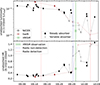 |
Fig. B.1. Zoom on the possible state transition during the decay of V4641 Sgr, with the two panels as in Fig. 1. Fully colored markers highlight the standard evolution obscured by a steady absorber, and transparent markers highlight the erratic and typically harder flux dipping periods interpreted as the sign of a second, variable absorber. We note that the 6−10/3−6 keV hardness ratio does not fully encompass the spectral evolution of the dipping observations. |
Appendix C: Resolve branching ratios
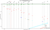 |
Fig. C.1. Branching ratios of all Resolve pixels in the 2−12 keV band, identified by count rate (bottom) and the identification number of each pixel. Diamonds show the observed values and lines the theoretical prediction. The theoretical values for Mp and Ms (blue and cyan) and Lp and Ls (orange and red) are identical in this range of count rates. We highlight in red pixel number 27, which was not included in our analysis. |
Appendix D: Spectral analysis
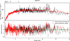 |
Fig. D.1. Unfolded spectra and residuals for the time-averaged products of Resolve (black) and Xtend (red). We use the best-fit absorbed disk blackbody model described in Table 1, with all line components removed. In all panels, the Resolve spectra are further binned at a 2σ significance level. |
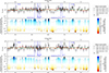 |
Fig. D.2. Blind searches showing the significance of the residuals after the Gaussian fit (top) and the pion fit (bottom) in the most critical energy band. Due to the very high ratios (≳4) of the remaining emission features, the ratio panels are shown in log scale. |
Evolution of spectral lines identified in the orbit-resolved Resolve spectra.
All Tables
Significant spectral lines identified in the time-averaged Resolved+Xtend spectra.
Best-fit continuum parameters for the individual orbits using a partially covered disk model.
All Figures
|
Fig. 1. Long-term monitoring of V4641 Sgr with different instruments during the 2024 outburst. From top to bottom: (first) MAXI daily light curve in the 2–10 keV band, obtained via PSF fitting (black), and generated via the MAXI on-demand interface (gray). See Sect. 2.2.1 for details. (Second) Einstein probe light curve in the 0.5–4 keV band. (Third) NICER/Swift/XRISM 1–10 keV luminosity light curves in Eddington units, after removal of the ISM absorption component. (Fourth) NICER/Swift/XRISM 6–10/3–10 keV hardness ratio (HR) evolution. The results in the last two panels come from fitting the time-integrated spectra of the individual ObsIDs in this period (see Sect. 2.2 for more details). The blue and red lines highlight the radio observations reported in Grollimund et al. (2024a,b), and the green line the XRISM and simultaneous Seimei observations. |
| In the text | |
|
Fig. 2. Zoom of the unfolded Resolve and Xtend spectra in the 6.2−7.2 keV band after the continuum modeling, highlighting the presence of strong emission features. The spectra are rebinned visually at a 2σ significance level for illustrative purposes. |
| In the text | |
|
Fig. 3. Residuals of the Resolve unfolded time-averaged spectra with the model of photo-ionized plasma emission (red) and the numerical MC radiative transfer simulation (blue). These two models are fitted simultaneously to the Xtend and Resolve data, with the Xtend data omitted from the plot for clarity. |
| In the text | |
|
Fig. 4. Left: Xtend light curve and HR of the observation with bins of 128 s, highlighting the different orbits used for time-resolved spectroscopy. Right: Folded Xtend and Resolve spectra of individual orbits of the observation (top) and zoom of Resolve to the 6.3−7.3 keV band (bottom) rebinned for visual clarity. |
| In the text | |
|
Fig. 5. Optical spectrum obtained with the Seimei telescope. The blue and black data show the spectra obtained with the VPH-495 and VPH-683 grisms, respectively. Finally, ⊕ indicates the atmospheric lines. |
| In the text | |
|
Fig. 6. Most relevant spectral lines in the donor (top) and Seimei (bottom) spectra and empirical best-fit models. In the Seimei spectra, the contributions of the individual components are indicated by dashed lines. |
| In the text | |
|
Fig. B.1. Zoom on the possible state transition during the decay of V4641 Sgr, with the two panels as in Fig. 1. Fully colored markers highlight the standard evolution obscured by a steady absorber, and transparent markers highlight the erratic and typically harder flux dipping periods interpreted as the sign of a second, variable absorber. We note that the 6−10/3−6 keV hardness ratio does not fully encompass the spectral evolution of the dipping observations. |
| In the text | |
|
Fig. C.1. Branching ratios of all Resolve pixels in the 2−12 keV band, identified by count rate (bottom) and the identification number of each pixel. Diamonds show the observed values and lines the theoretical prediction. The theoretical values for Mp and Ms (blue and cyan) and Lp and Ls (orange and red) are identical in this range of count rates. We highlight in red pixel number 27, which was not included in our analysis. |
| In the text | |
|
Fig. D.1. Unfolded spectra and residuals for the time-averaged products of Resolve (black) and Xtend (red). We use the best-fit absorbed disk blackbody model described in Table 1, with all line components removed. In all panels, the Resolve spectra are further binned at a 2σ significance level. |
| In the text | |
|
Fig. D.2. Blind searches showing the significance of the residuals after the Gaussian fit (top) and the pion fit (bottom) in the most critical energy band. Due to the very high ratios (≳4) of the remaining emission features, the ratio panels are shown in log scale. |
| In the text | |
Current usage metrics show cumulative count of Article Views (full-text article views including HTML views, PDF and ePub downloads, according to the available data) and Abstracts Views on Vision4Press platform.
Data correspond to usage on the plateform after 2015. The current usage metrics is available 48-96 hours after online publication and is updated daily on week days.
Initial download of the metrics may take a while.