


| Issue |
A&A
Volume 710, June 2026
|
|
|---|---|---|
| Article Number | A359 | |
| Number of page(s) | 29 | |
| Section | Planets, planetary systems, and small bodies | |
| DOI | https://doi.org/10.1051/0004-6361/202557276 | |
| Published online | 29 June 2026 | |
Volatile-bearing mineral atmospheres of hot rocky exoplanets as probes of interior state and composition
1
ETH Zürich, Department of Earth and Planetary Sciences, Institute for Geochemistry and Petrology,
Zürich,
Switzerland
2
Universität Bern, Center for Space and Habitability,
Bern,
Switzerland
3
Universität Bern, Physikalisches Institut, Weltraumforschung und Planetologie,
Gesellschaftsstrasse 6,
3012
Bern,
Switzerland
★ Corresponding author: This email address is being protected from spambots. You need JavaScript enabled to view it.
Received:
16
September
2025
Accepted:
30
March
2026
Abstract
Context. Spectra collected by the James Webb Space Telescope (JWST) hint at a volatile-rich and perhaps CO/CO2-bearing atmosphere on the hot rocky exoplanet (HRE) 55 Cancri e. Such atmospheres, should they persist, are thought to be products of mass exchange with underlying magma oceans and thereby carry an imprint of the geochemical state of HREs.
Aims. Here, we aim to identify diagnostic features in emission and transmission that can be used to infer the composition and geochemical state of HREs.
Methods. We constructed a coupled atmosphere-interior model that computes the equilibrium gas speciation in the system Si–Mg–Fe–O–C–H–S–N–He. The model accounts for both the equilibrium vaporisation of mineral gases and the partitioning of volatile species between the magma ocean and atmosphere. Using a fiducial planet with the properties of 55 Cancri e, we explored a parameter space that spans volatile mass fractions from 0.1 to ten times that of the Earth, solar- to Earth-like metallicities, and oxygen fugacities (fO2) −6 to +6 log10 units relative to the iron-wüstite (IW) buffer.
Results. We find the fO2 of the mantle to be the major control on emission and transmission spectra. At low fO2 (ΔIW < −3), SiO and CO appear in both emission and transmission. Between −3 < ΔIW < +3, CO and CO2 dominate infrared spectra. At high fO2 (ΔIW ≥ +3), CO2 in high-metallicity atmospheres is joined by SO2, producing strong absorption at 9 μm. H2O features appear in all ΔIW > −3 atmospheres, but are sensitive to H2 content. Condensation of silicates and iron oxides is common in the upper atmospheres of oxidised planets and is driven by cooling from triatomic molecules. Observed mass–radius trends suggest that a substantial fraction of HREs, including 55 Cancri e, have modest atmospheres of mixed heritage that are degenerate in fO2, volatile mass, and metallicity. Combined with JWST Mid-Infrared Instrument observations, high metallicity (Earth-like) atmospheres as well as highly reduced solar-like atmospheres are precluded on 55 Cancri e, while the Near Infrared Camera data remain inconclusive. Future observations at wavelengths beyond 8 μm are key to discerning between potential scenarios.
Key words: planets and satellites: atmospheres / planets and satellites: interiors / planets and satellites: terrestrial planets
© The Authors 2026
 Open Access article, published by EDP Sciences, under the terms of the Creative Commons Attribution License (https://creativecommons.org/licenses/by/4.0), which permits unrestricted use, distribution, and reproduction in any medium, provided the original work is properly cited.
This article is published in open access under the Subscribe to Open model. This email address is being protected from spambots. You need JavaScript enabled to view it. to support open access publication.
1 Introduction
Hot rocky exoplanets (HREs) denote a class of ultra-short period exoplanets that are similar in density to those of the terrestrial planets of the Solar System, implying an interior structure dominated by a rocky mantle and a core of iron-nickel alloy. Unlike the terrestrial planets, they have dayside temperatures (Tday) in excess of the melting point of silicates (≳1000 K). They usually exceed Earth in mass and radius (Luque & Pallé 2022), thus forming a subset of the Super-Earth population, and revolve on tight orbits around their host stars usually at a distance of a few stellar radii, dorb ~ 2–10R⋆). Consequently, also owing to the age of the stellar system in which they occur, these planets are likely to be tidally locked (Léger et al. 2011), resulting in the day side likely showing extreme hot spots even in the presence of atmospheres (Hammond & Pierrehumbert 2017; Zhang & Showman 2017). Hot rocky exoplanets are also numerous. Today, roughly 1000 candidates with substellar temperatures above 1000 K have been identified (Zilinskas et al. 2022).
Though their densities are broadly consistent with an interior structure similar to that of Earth (Zeng et al. 2016), the range permits planets with large metallic cores akin to Mercury (Adibekyan et al. 2021), while others have uncompressed densities lower than Earth’s and thus could harbour a smaller core (Elkins-Tanton & Seager 2008), a gaseous or supercritical water-rich layer (e.g. Aguichine et al. 2021), or a (comparatively) thick atmosphere (Peng & Valencia 2024); for some, only the last two options are consistent with their low density.
Recent observations with the James Webb Space Telescope (JWST) of the old (8.6±1 Gyr, Bourrier et al. 2018) HRE 55 Cancri e indicate the possible existence of an atmosphere (Hu et al. 2024; Patel et al. 2024) that appears compatible with a CO/CO2 composition (Hu et al. 2024), supporting earlier claims based on data from the Spitzer Space Telescope (Demory et al. 2016a,b). Other potential HRE candidates are TOI-431 b (Monaghan et al. 2025) and TOI-561 b (Teske et al. 2025), showing lower than expected day-side emission consistent with heat-redistribution by an atmosphere. Therefore, despite the likelihood of atmospheric escape owing to the high degree of stellar irradiation experienced by HREs (e.g. Salz et al. 2016; Cherubim et al. 2025), volatile-rich atmospheres appear to persist.
If present, the atmosphere may act as a thermal blanket for the interior, sustaining a deep molten magma ocean over its lifetime (Nicholls et al. 2024, 2025b). The high temperatures further facilitate short chemical reaction timescales (Arrhenius 1889), implying that the chemistry of the atmosphere should adjust to the thermochemical conditions of the mantle, provided the mass of the atmosphere is small compared to the reservoir of chemically active melt (Seidler et al. 2024; otherwise, the mantle and atmosphere tend to a common equilibrium; see e.g. Schlichting & Young 2022). Physically, this equilibrium manifests as the mutual solubility of volatile and silicate liquid components at the magma ocean–atmosphere interface (MAI). Volatile species that show particularly high solubilities in silicate liquids are water (Sossi et al. 2023), S-bearing gases (Boulliung & Wood 2022, 2023), and N2, provided N3− is stable in the liquid (Libourel et al. 2003; Dasgupta et al. 2022). As volatile-bearing gases dissolve in the magma, the atmospheric composition must change as a result (Sossi et al. 2020; Kite et al. 2020; Seo et al. 2024). In addition, evaporation of the underlying silicate melt releases gases such as SiO(g), Mg(g), and Fe(g), colloquially known as mineral gases. On dry (volatile-free) HREs, the mineral vapour may form an atmosphere on its own (e.g. Zilinskas et al. 2022; Seidler et al. 2024), but if volatiles are present, a mixed atmosphere emerges (Zilinskas et al. 2023; Charnoz et al. 2023; Piette et al. 2023; Van Buchem et al. 2025). Therefore, interactions at the MAI, which is likely not directly observable by telescopes, imposes the speciation and mass of the atmosphere at the interface, thereby permitting the nature of the underlying magma ocean to be inferred from observations of atmospheric spectra.
A handful of earlier studies have attempted to model mixed mineral-volatile atmospheres of HREs. Typically, they assumed injection of pre-formed silicate vapour into a volatile background gas, closing the chemical network a posteriori (Zilinskas et al. 2023; Piette et al. 2023). This approach, though instructive, is not thermodynamically self-consistent because the fO2 of the system after the addition of volatile elements (such as H and C) decreases due to consumption of O2 in the initial mineral atmosphere by H2O and CO/CO2 (cf. Falco et al. 2024). Therefore, the final fO2 will no longer correspond to the initial guess, which was used to determine the mass and composition of the mineral atmosphere. This is important because the equilibrium partial pressures of mineral gas species, such as SiO(g), depend on fO2 (Wolf et al. 2023; Seidler et al. 2024).
Later studies by Charnoz et al. (2023) and Falco et al. (2024) combined a stoichiometric vaporisation approach with titration of H2-gas into the system. The resulting speciation in the atmospheres is chemically and thermodynamcally self-consistent but imposes the condition that fO2 depends upon the amount of H2 gas titrated into the system, precluding a treatment of fO2 as an independent variable. This requirement arises because under the small-atmosphere approximation, the thermochemistry (including fO2) of the vapour should be set by the mantle, and the conserved quantity for gas species in exchange with the melt is therefore not their amount but their chemical potential, μ = μ0 + RT ln f, characterised by their fugacity, f, at a given temperature (μ0 is the chemical potential at the arbitrary reference state, typically 1 bar and the T of interest, where T is the temperature and R the is universal gas constant). As shown in Seidler et al. (2024) (their Eq. (8)), the fugacity of a mineral gas species is a function of the thermodynamic activity, a, of the parent species1 and the oxygen fugacity:
![Mathematical equation: $\[f \propto a^\alpha(P, T, x_{m e l t}) \cdot f \mathrm{O}_2^\beta,\]$](/articles/aa/full_html/2026/06/aa57276-25/aa57276-25-eq1.png) (1)
(1)
where α and β are constants depending solely on the stoichiometry of the vaporisation reaction.
The importance of fO2 is further demonstrated in pure volatile atmospheres, wherein the speciation shifts from reduced components such as CO and H2 to oxidised CO2 and H2O (Sossi et al. 2020), and the solubility of N2 and S2 increase significantly as fO2 decreases (Libourel et al. 2003; Bernadou et al. 2021; Boulliung & Wood 2022, 2023). Correspondingly, the atmospheric signature should change; in particular, the strong increase in SO2 partial pressure and its high opacity make it an excellent probe in emission spectra for the redox state of magma ocean atmospheres in planets with an Earth-like volatile budget (Hu et al. 2024; Bello-Arufe et al. 2025; Nicholls et al. 2025b). However, the degree to which its intensity varies as a function of the partial pressures of other gases has yet to be explored. Moreover, depending on the extent to which mineral gases evaporate, the production of new species occurs, such as silane (SiH4), in atmospheres of solar-like composition under reducing conditions (Charnoz et al. 2023).
The mantle redox state, as expressed by fO2, is expected to exert crucial controls on the atmospheric composition. Inversion thereof can be used to constrain information about the hidden interior. Yet a systematic and self-consistent treatment of how the presence of volatile elements interact with mineral species in the presence of a magma ocean have not been performed with self-consistent thermodynamics. Such models are crucial for identifying degeneracies in atmospheric retrievals of fO2, volatile mass fractions, and metallicities of HREs as well as diagnostic signals thereof.
Here, we present a coupled interior-atmosphere model that computes the key observable properties of volatile-bearing HREs of a given mass: their radius, Rp; the emission and transmission spectra as function of the fO2 at the magma oceanatmosphere interface; the volatile mass fraction (VMF); and the metallicity of volatile elements (ξ). In Section 2, we introduce this model, and we investigate the main results in Section 3, where we present a systematic investigation of the atmospheric mass and speciation as function of fO2, VMF, and ξ as well as the structure and emission and transmission spectra of these atmospheres. We relate our models to the observed properties, notably mass-radius and spectral observations, where available, of HREs in Section 4. Finally we conclude and summarise our work in Section 5, where we also highlight our assumptions and caveats.
2 Methods
2.1 Model pipeline
The coupled atmosphere-interior model is composed of two main components, (a) the (independent) model for computing the speciation and mass of gaseous species and dissolved components at the MAI, Atmodeller2 (Bower et al. 2025), and (b) the (dependent) radiative transfer pipeline phaethon3 (Seidler et al. 2024) that computes the speciation and structure of the overlying atmosphere layer-by-layer based on the input boundary conditions at the MAI (step a.) and the top of the atmosphere (TOA). In order to ensure consistency, steps a.) and b.) have to be brought into equilibrium, that is, the temperature at the MAI (TMAI) must match the temperature at the bottom of the atmosphere (TBOA) computed by the radiative transfer calculation for a given Tirr, for which an iterative computation is required. The components of the pipeline are explained in more detail below.
2.1.1 Atmosphere-interior equilibrium model
The fundamental assumption of the atmosphere-interior model is that the melt and gas are at chemical equilibrium. A precise statement of this condition is that the chemical potential (μ) of any species (i) in the melt must equal that in the gas,
![Mathematical equation: $\[\mu_{i, \text {melt }}=\mu_{i, \text {gas}},\]$](/articles/aa/full_html/2026/06/aa57276-25/aa57276-25-eq2.png) (2)
(2)
as it enables the partitioning of species between mantle and atmosphere to be derived by linking their fugacities (effective pressures) in the gas phase with their activities (effective concentrations) in the melt, which is performed by Atmodeller via the extended law of mass action4.
We imposed two sets of constraints on the system of equations. First, we ensured mass conservation for each volatile element H, He, C, N, and S and thus their combined total mass. The individual masses were determined as described in Sect. 2.3.
The second set of constraints are the fugacities of species supplied by the magma ocean. The mantle, composed of molten silicates, is the largest reservoir of O in the system and can effectively act as an infinite reserve thereof. Hence, the masses of O2, the mineral gases, or any gas species containing oxygen as well as the total atmospheric mass are not conserved. Instead, we imposed the oxygen fugacity (fO2) as an independent variable, which is reported here relative to the iron–wüstite buffer IW, ΔIW := fO2(P, T) − IW(P,T), for which we used the formulation of Hirschmann (2021). The fugacities of the mineral species, here fSiO, fMg and fFe (one per included element; see Sossi et al. 2019), are set by the melt composition, fO2 and TMAI, and were computed using a modified version of the MAGMA code (Fegley Jr & Cameron 1987; Schaefer & Fegley Jr 2004; Seidler et al. 2024). The initially volatile-free melt is composed of SiO2, MgO and FeO in identical ratios to the bulk silicate Earth for all simulations (Palme & O’Neill 2013).
To evaluate partitioning of a (volatile) species i (e.g. CO2, H2O) between mantle and atmosphere via a solubility law, its fugacity fi at the MAI has to be found. Fugacity relates to the partial pressure pi via an equation of state, taken here as the ideal gas law (for which fi = pi), that in turn hinges on the radius of the planet at the interface (i.e. Rp,MAI), the surface gravity (gMAI), the species atmospheric mass (Mi), its molecular weight (mi), and the average mean molecular weight (MMW) of the atmosphere (![Mathematical equation: $\[\bar{m}\]$](/articles/aa/full_html/2026/06/aa57276-25/aa57276-25-eq3.png) ; Bower et al. 2019):
; Bower et al. 2019):
![Mathematical equation: $\[f_i=p_i=\frac{M_i \cdot g_{\mathrm{MAI}}}{4 \pi R_{p, \mathrm{MAI}}^2} \cdot \frac{\bar{m}}{m_i}.\]$](/articles/aa/full_html/2026/06/aa57276-25/aa57276-25-eq4.png) (3)
(3)
Internally, some of these quantities are further related by the temperature at the interface, TMAI · Rp,MAI and gMAI are computed from the mass of the planet, Mp, and its core mass fraction (CMF) by interior structure models for rocky planets (Zeng et al. 2016). The effect of dissolved volatiles on the density of the planet is neglected. As shown a posteriori (Sect. 3.1), the concentration of water – the most soluble species – reaches, at most, 3 wt%, for which we estimate a density decrease of ~0.1 g cm−3 (Matsukage et al. 2005; Dorn & Lichtenberg 2021). Relative to differences in mass-radius induced by atmospheric extent, the effect of H2O is likely negligible; indeed, Boley et al. (2023) found no major change in planet density even when incorporating 5.2 wt% of water. Additionally, we ignore the density difference introduced by melting of the mantle. Again, the density difference between a fully molten and fully solid mantle becomes small for planets with Mp ≳ 2.7 M⊕ (~2% in density ⇔~ 0.7% in radius, Boley et al. 2023), but might be relevant for Earth-sized planets (~11.1% in density ⇔ ~3.7% in radius; Boley et al. 2023; Bower et al. 2019), though this remains small compared to variations induced by atmospheric properties. Unless mentioned otherwise, the mass is kept constant at Mp = 8 M⊕ to mimic that of 55 Cancri e (Bourrier et al. 2018). To study Earth-like interiors only, we keep CMF=0.325 throughout. With these parameters we obtain Rp,MAI = 1.74 R⊕. The melt mass is internally computed by Atmodeller from the mantle melt fraction xmelt and the total mantle mass, Mmelt = xmelt · Mp(1 – CMF). Because our model ignores any volatile species that can be incorporated into solids, Mmelt defines the effective mass into which volatile elements may dissolve. Throughout this study, assume a fully molten mantle, xmelt = 1. Lower melt fractions are not expected to substantially modify the atmospheric composition unless xmelt ≲ 0.3 (Bower et al. 2022; Maurice et al. 2024). The melt fraction of volatile rich HREs are expected to be ≳0.75, as the planets struggle to cool under the intense irradiation (Nicholls et al. 2024).
The set of desired target gas species (including species of both mineral and volatile gases) is added to Atmodeller together with their respective solubility laws, if available (Bower et al. 2025). The full list of gas species, including their solubility laws, can be found in Table A.1. Atmodeller then solves for the mass distribution and partial pressures of all species given the aforementioned constraints. Once all the partial pressures (and thus the total pressure), together with the dissolved quantities in the melt is known, its output is passed on to the radiative model (see next Sect. 2.1.2). If Atmodeller detects the formation of condensates, the condensate mass is removed and the atmospheric composition is calculated from the remaining gas mass. Here, only graphite is considered due to the high temperature at the MAI.
2.1.2 Radiative transfer model
To match TMAI with TBOA and find the equilibrium atmospheric pressure, structure and chemistry, we integrate the outgassing model into the radiative transfer pipeline phaethon. It operates as follows:
The energy budget of the planet is determined from the imposed irradiation temperature Tirr. The atmospheric P–T-structure for a given bulk composition and intrinsic temperature (see point 5, below) depends only on the incoming spectral energy distribution (SED), given in W m−2 μm−1. In integrated form, this is reasonably well approximated by the Stefan-Boltzmann law,
![Mathematical equation: $\[\sigma T_{\mathrm{irr}}^{4}\]$](/articles/aa/full_html/2026/06/aa57276-25/aa57276-25-eq5.png) , where Tirr is the irradiation temperature at the TOA. Thus, planets with identical Tirr (and identical atmospheric composition) have identical atmospheric structures for equal stellar SEDs, regardless of other characteristics (e.g. stellar radius R⋆ or orbital separation d between star and planet).
, where Tirr is the irradiation temperature at the TOA. Thus, planets with identical Tirr (and identical atmospheric composition) have identical atmospheric structures for equal stellar SEDs, regardless of other characteristics (e.g. stellar radius R⋆ or orbital separation d between star and planet).Initially, we set TMAI to Tirr. Alternatively, an informed initial guess can be given to accelerate convergence.
The atmospheric elemental abundances as well as the pressure at the MAI (PMAI) are computed by the atmosphereinterior model (Sect. 2.1.1) using the current TMAI, and passed to the radiative transfer routine as constraints.
FastChem COND (Kitzmann et al. 2024) is used to calculate look-up tables for the gas speciation as function of pressure and temperature (i.e. altitude), assuming that the gas retains the elemental composition set at the MAI throughout the atmospheric column, and that thermochemical equilibrium is established at every layer. This additionally assumes that the reaction timescale is negligibly short compared to the timescale of vertical diffusion of molecular species, for example by quenching, an assumption that is supported by the (expected) high temperatures of the atmosphere. We allowed for the formation of condensates but did not separate them from the gas (equilibrium condensation mode, as opposed to the rainout mode which would permanently remove condensing elements). The spectral properties of condensates, as either clouds or hazes, are ignored during the radiative transfer computation. All included gas and condensate species are listed in Table A.2.
-
HELIOS (Malik et al. 2017, 2019) derives the P–T-structure of the atmosphere, including a new value for TBOA, by solving the equations of radiative transfer using the opacities of the individual gas species and the chemistry determined in step 4. The atmosphere is plane-parallel and confined between the top-of-the-atmosphere pressure (PTOA, fixed at 10−8 bar) and bottom-of-the-atmosphere pressure (PBOA = PMAI, computed by the outgassing model, step 3). The energy budget is characterised by Tirr (step 1); however, HELIOS internally operates on the physical parameters of the star–planet system. Therefore, we fix the properties of the star to solar values, R⋆ = R⊙, and take the spectrum from Gueymard (2004). The orbital distance is reconstructed from Tirr via
![Mathematical equation: $\[d=\sqrt{\hat{\mathfrak{f} \cdot\left(1-A_B\right)}} R_{\star}\left(\frac{T_{\star}}{T_{\mathrm{irr}}}\right)^2,\]$](/articles/aa/full_html/2026/06/aa57276-25/aa57276-25-eq6.png) (4)
(4)where AB is the bond albedo of the planet and 𝔣 is the dilution factor. We assume AB = 0 (black-body) and 𝔣 = 2/3 (ineffective heat redistribution; see Hansen 2008); as elucidated in point 1, neither the characteristics of the atmosphere nor the resulting emission and transmission spectra depend on these parameters. For the intrinsic temperature, we take a conservative estimate of Tint = 0 K. However, deviations therefrom have been shown to severely modify atmospheric structures of cooler lava planets, particularly by inducing convection (e.g. Nicholls et al. 2025a). Consequently, we independently examine the effect of Tint ∈ {200, 250, 300} K in Appendix F and justify the choice of Tint = 0 a posteriori. Convective adjustment is enabled with an adiabatic exponent for diatomic gases, κ = 2/7:
![Mathematical equation: $\[\frac{\mathrm{d} ~\ln~ T}{\mathrm{~d} ~\ln~ P}=\kappa:=-\frac{1-\gamma}{\gamma},\]$](/articles/aa/full_html/2026/06/aa57276-25/aa57276-25-eq7.png) (5)
(5)where γ is the adiabatic index which is 7/5 for a diatomic, ideal gas. The opacity is computed on-the-fly via the random-overlap method (Amundsen et al. 2017), using the mixing ratios of each layer inferred from the FastChem lookup tables (point 4). The selection of species opacities are outlined in Sect. 2.2.
If the new TBOA is within ΔTabstol of the prior guess of TMAI, the model is taken to have converged. Otherwise, a new TMAI is estimated via root-finding (see Appendix B.1), and the model repeats from step 3. We choose ΔTabstol = 35 K to minimise the number of calls to the computationally expensive radiative transfer solver, but find that most models converge with ΔT := TBOA − TMAI < 10 K or even < 2 K. We expect negligible differences in the results if the constraints were to be tightened.
Once converged, phaethon yields the atmospheric structure, surface pressure, gas speciation in each layer, and emission spectra. The latter cannot be used directly, as HELIOS does not take into account the wavelength dependent radius of the planet (based on the varying atmospheric opacity). phaethon therefore reconstructs the emission spectrum using the vertical structure and contribution function of the atmosphere (see Appendix B.2).
Transmission spectra were computed from the P-T-structure and chemistry with petitRADTRANS (Mollière et al. 2019). The opacity sources are kept the same.
2.2 Opacities
The introduction of volatiles to a silicate mineral atmosphere vastly expands the list of species for which opacities are required (Zilinskas et al. 2023, 2025). In most of our simulations, we use a selection that was optimised for accuracy and computational time and is based on the results from our speciation and radiative transfer simulations presented in Sect. 3. We obtained the raw opacity sources for the atomic and molecular species from the DACE5 or the former Exoclimes simulation platform, which hosted the data prior to their upload to DACE (no longer available at the time of publication). The opacities hosted on either were computed with HELIOS–K (Grimm & Heng 2015; Grimm et al. 2021) assuming Voigt profiles, and with a resolution of Δν = 0.01 cm−1. Molecular species have a line wing cut-off at 100 cm−1 from the core, whereas atomic species have none to preserve the shape of wide resonant lines (e.g. Mg at 285 nm). Collision-induced absorption (CIA) opacities were generated with HELIOS–K with the same specifications as the atomic and molecular opacities, using the data from HITRAN6.
The tables of correlated-k coefficients used by HELIOS were constructed from the raw opacities via the k-table program (part of HELIOS) using a resolution R := λ/Δλ = 200 in the wavelength range 0.18–200 μm. The detailed list of species is shown in Table D.1 and comprises the “active” absorbers SiO, MgO, Mg, Fe, CO2, CO, H2O, CH4, NO, SO, SO, HS, H2S, OH, O2, and HCN, in addition to the “inactive” H, He, N2 and H2. The latter do not show strong opacities (Fig. D.1), but may occur in large abundances and are therefore required by HELIOS to reproduce the proper MMW 7. C2H2 was not used as absorber due to limitations outlined in Appendix J. As Rayleigh scatterers, we allowed for O2, H2O, He, e−, H, N2, CO, CO2, and H2. For CIAs, only H2–H2, H2–He, H2–H and He–H were available at the temperatures of interest; since we found negligible influence on HRE spectra, we omitted them unless otherwise mentioned (Appendix E).
2.3 Volatile budget
2.3.1 Total volatile mass
We defined the volatile mass fraction (VMF) as the mass of H–He–C–N–S (MV) relative to the mass of the entire planet (MP):
![Mathematical equation: $\[\mathrm{VMF}:=\frac{M_V}{M_P}.\]$](/articles/aa/full_html/2026/06/aa57276-25/aa57276-25-eq8.png) (6)
(6)
For the Earth, VMF⊕ = 0.00028485 (Palme & O’Neill 2013). We further defined the volatile mass factor of any model planet by
![Mathematical equation: $\[\Psi_{\mathrm{VMF}}:=\log _{10}\left(\frac{\mathrm{VMF}}{\mathrm{VMF}_{\oplus}}\right),\]$](/articles/aa/full_html/2026/06/aa57276-25/aa57276-25-eq9.png) (7)
(7)
which represents the VMF of a planet of any mass, Mp, compared to that of Earth scaled up to Mp. That is, ΨVMF =0 if the planet has the same mass fraction of volatile elements as Earth (though these are not necessarily present in the same relative abundances; see Sect. 2.3.2). We caution that ΨVMF is not identical to the atmospheric mass fraction since oxygen is not included in its calculation. Instead, oxygen is a special case as it is set by a combination of ΨVMF, metallicity (see Sect. 2.3.2) and the fO2 of the mantle (for the same reason, we cannot use the atmospheric mass fraction as free parameter). We investigated ΨVMF ∈ {−1, 0, 1}, corresponding to 0.1, 1 and 10 times the Earth’s volatile budget in mass, respectively.
2.3.2 Mixing between solar and bulk-silicate Earth-like metallicities
Due to the computational demand of our forward model, and our inability to constrain the relative abundances of volatile elements in planetary bodies from stellar spectra in a similar vein to the major rock-forming elements (e.g. Wang et al. 2019, 2022; Spaargaren et al. 2023), we restrict ourselves to a more compact and efficient framework. To incorporate variations in He/H, C/H, N/H and S/H ratios into a single parameter, we define a mixing line between a composition that mimics a solar gas (SOLAR, Lodders 2021) and one that corresponds to the volatile budget in bulk silicate Earth (VIBSE, Palme & O’Neill 2013, their Table 4)8, for which we introduce the parameter ξ. It formally corresponds to the fraction of VIBSE-like material in the total amount of volatiles, where ξ =0 is SOLAR and ξ =1 denotes VIBSE. The mass ratios of volatiles relative to hydrogen, Φ := [He/H, C/H, N/H, S/H], are defined as
![Mathematical equation: $\[\boldsymbol{\Phi}_{\text {planet }}=\boldsymbol{\Phi}_{\mathrm{SOLAR}}+\xi \cdot\left(\boldsymbol{\Phi}_{\mathrm{VIBSE}}-\boldsymbol{\Phi}_{\mathrm{SOLAR}}\right),\]$](/articles/aa/full_html/2026/06/aa57276-25/aa57276-25-eq10.png) (8)
(8)
where the reference ratios can be found in Table 1. The mass fraction of the elements as function of ξ is shown in Fig. 1. Phosphorus, while often listed among the crucial volatiles for exoplanet atmospheres (Zilinskas et al. 2025), was not considered in this work due to a.) its low abundance in VIBSE (~87 ppm, Palme & O’Neill 2013) and b.) its comparatively low volatility compared to C–H–N–S (Gillmann et al. 2024).
Mass ratios of volatiles for the two endmember cases.
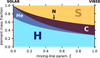 |
Fig. 1 Bulk volatile (mass) ratios of volatiles as a function of ξ. |
3 Results
3.1 Atmospheric and interior chemistry
The atmospheric and interior chemistry is set by exchange at the MAI, and thus determined by the atmosphere-interior equilibrium model (Sect. 2.1.1). We describe element speciation in the interior and atmosphere of a fully molten planet with Mp = 8 M⊕, Rp,MAI = 1.74 R⊕ and TMAI = 3000 K, which mimics the broad characteristics of 55 Cancri e (Mp = 7.99 ± 0.33 M⊕ and Rp = 1.875 ± 0.029 R⊕, Bourrier et al. 2018, and TMAI ~ 3000 K in accordance with later findings; see Sect. 3.2). We examine variations in the surface partial pressures at the MAI (Fig. 2) and in the elemental mass fractions in the atmosphere relative to that dissolved in the mantle (Fig. 3) as a function of the three independent variables investigated in this work: ΨVMF, ξ and fO2.
3.1.1 Helium
Helium is abundant in low-ξ (SOLAR) atmospheres, with the vast majority of its inventory remaining in the atmosphere (>90%; see Fig. 3; melt concentrations are <0.07 wt% over the tested range). This reflects its low solubility, based on mechanical incorporation into interstitional sites in the melt structure (Carroll & Draper 1994). Its solubility law is therefore independent of fO2, yet, there is an apparent dependence of pHe on ΔIW in Fig. 2, which arises due to evolving ![Mathematical equation: $\[\bar{m}\]$](/articles/aa/full_html/2026/06/aa57276-25/aa57276-25-eq11.png) of the atmosphere with fO2, particularly affecting light gases such as He (cf. Eq. (3)). The changes in
of the atmosphere with fO2, particularly affecting light gases such as He (cf. Eq. (3)). The changes in ![Mathematical equation: $\[\bar{m}\]$](/articles/aa/full_html/2026/06/aa57276-25/aa57276-25-eq12.png) are driven by Si-outgassing in reducing and O2-formation in oxidising atmospheres (see Sects. 3.1.6 and 3.1.7). Consequently, increased pHe leads to greater dissolution of He under these conditions (Fig. 3).
are driven by Si-outgassing in reducing and O2-formation in oxidising atmospheres (see Sects. 3.1.6 and 3.1.7). Consequently, increased pHe leads to greater dissolution of He under these conditions (Fig. 3).
3.1.2 Hydrogen
We recovered the fO2-dependent behaviour of the partial pressures of the major hydrogen gases H2 and H2O found in earlier studies (Sossi et al. 2020; Gaillard et al. 2022). While pH2O/pH2 is proportional to fO2 0.5, the high solubility of water (as OH− Sossi et al. 2023; Thompson et al. 2025) relative to H2 (as H2, Hirschmann et al. 2012; Foustoukos 2025; Chaudhari et al. 2025) means that pH2 reaches higher limits than does pH2O, by ~1–2 orders of magnitude. Correspondingly, the atmospheric H content becomes a strong function of fO2, with expected H contents an order of magnitude greater in reducing (ΔIW≲0) than in oxidising atmospheres.
Relative to its atmospheric abundance, H is almost always more concentrated in the mantle, especially under oxidised conditions (Fig. 3). This leads to comparatively high concentrations, up to ~0.5 wt% of H2O in the melt for ΨVMF ≲1; in volatile-rich and intermediate-to-oxidised systems (ΨVMF = 1, ΔIW ≥ 0), concentrations of up to 3 wt% are reached. Although Fig. 3 shows lower H fractions in mantles in equilibrium with SOLAR-like metallicity (ξ) atmospheres, they actually contain higher absolute concentrations of H2O than for ξ =1 (VIBSE) cases, roughly by a factor of ~2. This is because the total hydrogen budgets are higher in SOLAR than in VIBSE cases (Fig. 1).
Water and hydrogen are the two dominant H-bearing gas species for most of the explored parameter space. Another important hydrogen carrier, CH4, only achieves a low partial pressure at the MAI temperatures of HRE atmospheres. However, it becomes the most abundant H-bearing gas for cases with VIBSE-like ξ and high ΨVMF (>1; Fig. G.1), owing to the homogeneous equilibrium:
![Mathematical equation: $\[3 \mathrm{H}_2(\mathrm{g})+\mathrm{CO}(\mathrm{g})=\mathrm{CH}_4(\mathrm{g})+\mathrm{H}_2 \mathrm{O}(\mathrm{g}),\]$](/articles/aa/full_html/2026/06/aa57276-25/aa57276-25-eq13.png) (9)
(9)
which proceeds to the right at high pressures. It should be noted, however, that the total pressure in such atmospheres exceeds 1 GPa, leading to non-ideal behaviour of gases (e.g. Bower et al. 2025; Hakim et al. 2026).
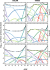 |
Fig. 2 Partial pressures of gas species at the magma ocean–atmosphere interface (MAI) as function of fO2, ΨVMF, and ξ. All atmospheres were simulated at TMAI = 3000 K and Mp = 8 M⊕. |
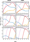 |
Fig. 3 Faction of the budget of a given element E ∈ {H, He, C, N, O, S} that resides in the atmosphere (Eatmo/Etotal), where “total” refers to the mass-weighted sum of atmosphere plus mantle. The dotted black line, log10-zero, denotes the level at which the entirety of an element would reside in the atmosphere. |
3.1.3 Carbon
Neither member of the CO–CO2 redox pair has a high solubility in silicate melts (Dixon et al. 1995; Yoshioka et al. 2019), nor does CH4 (Ardia et al. 2013); out of those, CO2 is the most soluble under intermediate to oxidising conditions (ΔIW > 0) and may reach concentrations of up to ~0.15 wt% in ΨVMF =1 atmospheres (CO <0.01 wt%, CH4 <0.0014 wt%). As a result, the majority of the carbon budget of a given planet resides in the atmosphere (Fig. 3). Therefore, a nearly continuous transition with similar pCO to pCO2 occurs with increasing fO2 0.5 at constant ΨVMF. For constant fO2, carbon may also precipitate as graphite, provided the partial pressure of CO is sufficiently high:
![Mathematical equation: $\[\mathrm{CO}(\mathrm{g})=\mathrm{C}(\mathrm{cr})+\frac{1}{2} \mathrm{O}_2(\mathrm{g}).\]$](/articles/aa/full_html/2026/06/aa57276-25/aa57276-25-eq14.png) (10)
(10)
This shows as a sharp decrease in the partial pressures of carbon-bearing gases, mainly CO, under reducing conditions (Fig. 2). As illustrated in Eq. (10), graphite precipitation occurs when the system is reducing (i.e. low fO2) and/or rich in carbon (i.e. high ξ and ΨVMF). Because the condensation of C(cr) is arrested by the formation of methane (Eq. (9) shifts to the right, meaning Eq. (10) shifts to the right), C precipitation does not occur in low ξ atmospheres (Fig. 2, also Fig. G.1).
In highly reducing (ΔIW ≲ − 3) and heavy atmospheres (ΨVMF ≳1), methane might replace CO as the dominant C-bearing gas species. Owing to the entropy change of Eq. (9), this exchanges is more pronounced in cooler temperatures (≲2000 K) due to the enhanced stability of methane; cold and highly reducing HREs could therefore also harbour methanerich atmospheres even for ΨVMF < 1 (cf. Liggins et al. 2022). However, the production of CH4 (and C-bearing gases more generally) is, to some degree, stifled in high H/C atmospheres (SOLAR) owing to a lack of carbon availability.
3.1.4 Sulfur
Aside from gases in the C–O–H(–He) system, which otherwise dominate the speciation of the atmospheres of HREs, S-bearing species may become abundant under certain, oxidising conditions (Gaillard et al. 2022; Gillmann et al. 2024). This is also borne out in our study, in which SO2 is the dominant species in the VIBSE case near ΔIW+3 (Fig. 2). Briefly, this arises because the solubility of S2 depends on fO2 (O’Neill & Mavrogenes 2002; Boulliung & Wood 2022, 2023) which manifests as two competing limits: under reducing conditions (ΔIW ≲0), nearly all sulfur is dissolved as S2− in the silicate melt, substituting for oxygen (Boulliung & Wood 2023), whereas under highly oxidising conditions, it dissolves predominantly as S6+ in the ![Mathematical equation: $\[\mathrm{SO}_{4}^{2-}\]$](/articles/aa/full_html/2026/06/aa57276-25/aa57276-25-eq15.png) moiety (Boulliung & Wood 2022). Compared to water, its dissolved concentration remains low: ≲0.025 wt% of S2-equivalent resides in the melt for ΨVMF ≲1, while under ΨVMF =1, the maximum concentration reached is ~0.2 wt%. Roughly around ΔIW+3, there exists a maximum where sulfur accumulates in the atmosphere (~60–100% of all S in the gas phase, cf. Fig. 3) and S-rich gases, particularly SO2, become the dominant species (see Hughes et al. 2023, for a detailed thermodynamic explanation). Other sulfur-bearing gases are not as important, but SO is found to accompany SO2 when the latter is abundant, and H2S is a minor species under very high ΨVMF (≥1), high ξ and reducing conditions, reaching mixing ratios of up to 5% (with the caveat again that these atmospheres are likely to be non-ideal). All else being equal, high-ξ (VIBSE) cases host greater concentrations of S in their mantles, typically ≳2 times higher than in low-ξ (SOLAR), and this maximum increases with ΨVMF.
moiety (Boulliung & Wood 2022). Compared to water, its dissolved concentration remains low: ≲0.025 wt% of S2-equivalent resides in the melt for ΨVMF ≲1, while under ΨVMF =1, the maximum concentration reached is ~0.2 wt%. Roughly around ΔIW+3, there exists a maximum where sulfur accumulates in the atmosphere (~60–100% of all S in the gas phase, cf. Fig. 3) and S-rich gases, particularly SO2, become the dominant species (see Hughes et al. 2023, for a detailed thermodynamic explanation). Other sulfur-bearing gases are not as important, but SO is found to accompany SO2 when the latter is abundant, and H2S is a minor species under very high ΨVMF (≥1), high ξ and reducing conditions, reaching mixing ratios of up to 5% (with the caveat again that these atmospheres are likely to be non-ideal). All else being equal, high-ξ (VIBSE) cases host greater concentrations of S in their mantles, typically ≳2 times higher than in low-ξ (SOLAR), and this maximum increases with ΨVMF.
3.1.5 Nitrogen
The partial pressure of N2 is sensitive to fO2 because it dissolves preferentially in the silicate melt under highly reducing conditions (ΔIW ≲−3), at which N3− is stable (Libourel et al. 2003; Bernadou et al. 2021). Consequently, highly reduced atmospheres are likely to be nitrogen-depleted relative to oxidised atmospheres (Shorttle et al. 2024) (Fig. 3). Therefore, even at high H/C ratios, the formation of gaseous ammonia, a reducing species, is inhibited, a result compounded by its thermal instability at the temperatures of HRE atmospheres. Gaseous nitrogen therefore mostly occurs as N2(g), with oxidising atmospheres (ΔIW ≳ +3) potentially forming nitrous oxide, NO(g), in similar or greater quantities than N2(g).
3.1.6 Mineral gases and hydrides – SiO, Mg, Fe, SiH4
The partial pressures of the mineral gases are set by the melt activities and fO2 (Eq. (1)) and thus behave like their dry lava planet counterparts (cf. Seidler et al. 2024). In atmospheres with bulk silicate Earth-like amounts of volatiles (ΨVMF =0), their partial pressures remain low and only approach those of the major volatiles (~100 bar) under highly reducing conditions (ΔIW ≲ − 5). This remains true even when the planetary mass is scaled down, as the total pressure remains of the order of 100 bar for planets with Mp ≥ 1 M⊕, to which the mineral gases contribute less than 1–10 bar (Seidler et al. 2024) for ΔIW >−4. For mineral gases to dominate, the planet must be depleted in volatiles (ΨVMF ≪ 0), highly reducing, or extremely hot such that evaporation of mineral gases is promoted (Wolf et al. 2023; Seidler et al. 2024). The transition from mineral-dominated to volatile-dominated atmospheres is therefore highly case dependent.
Metal hydrides such as SiH4 (silane), MgH, FeH or hydroxides (MgOH) are only minor constituents of most atmospheres; only under very reducing (ΔIW ≲ − 4) and massive (ΨVMF ≳ 1) atmospheres does silane emerge (Fig. G.1. Its stability is, however, only weakly dependent on ξ). It overtakes H2 as the dominant species below ΔIW = −5 for ΨVMF ~ 2. However, at these conditions, the total atmospheric pressure reaches 10s of GPa, well beyond the applicability of the ideal gas law and is more typical of the Sub-Neptune regime (Charnoz et al. 2023; Misener et al. 2023; Seo et al. 2024; Hakim et al. 2026).
3.1.7 Oxygen
Highly oxidising atmospheres (ΔIW ≳ + 5) are dominated by free O2. The fO2 (relative to IW) at which O2 becomes the most abundant gas species increases with decreasing temperature since the IW buffer (Fe + 1/2O2 = FeO) fixes higher pO2 (or fO2) at higher temperature. While we do not explicitly track the total amount of oxygen as it is instead set by the fO2, we can reconstruct its share between the atmosphere and mantle by assuming the mantle abundance of oxygen is given by the amount of dissolution-sequestered O by oxygen-bearing species (H2O, CO2 and CO) together with the 44.33 wt% oxygen residing in mantle silicates (Palme & O’Neill 2013). We find that the atmospheres studied here have ≪1 wt% of their entire oxygen budget in the gas (Fig. 3), a limit that is only reached under highly oxidising conditions; planets with ΨVMF ≤ 0 generally host ≪1 ‰ of their oxygen budget in their atmosphere, validating the notion that magma oceans buffer the atmospheric fO2.
3.2 Thermal structure and opacity
3.2.1 Phenomenology
In Fig. 4, we show the detailed atmospheric wavelength-dependent optical-depth (subpanel 1), temperature profile (subpanel 2), and mixing ratios of abundant gas species as a function of pressure (altitude, subpanel 3), organised in four archetypal planetary states; A – SOLAR oxidised (ΔIW+3), B – SOLAR reduced (ΔIW-3), C – VIBSE oxidised (ΔIW+3), D – VIBSE reduced (ΔIW-3). Each was calculated assuming a synthetic, fully molten archetype similar to 55 Cancri e, as outlined in Sect. 2.1.1 (8 M⊕, average dayside temperature Tirr = 2500 K). Here, only cases for an Earth-like amount of volatiles (ΨVMF =0) are shown.
Many of the dominant gas species, namely CO2 and H2O, are classical greenhouse gases that cause heating in the lower atmosphere due to entrapment of outgoing infrared emission (e.g. Ledley et al. 1999), but cooling in the upper layers due to efficient emission in the same wavelength bands (e.g. Bougher et al. 1999). Thus, most of the simulated atmospheres show a notable greenhouse effect up to 500 K in conjunction with an upper atmosphere (P ≲ 0.1 bar) that can be 500–1000 K cooler than the irradiation temperature, particularly for the VIBSE cases (Fig. 4, C2, D2). The major gas species maintain a roughly constant mixing ratio throughout the atmospheric column, in spite of changing temperatures (ΔT ~ 1000 K) as discussed above. Only when the atmosphere shows a thermal inversion (i.e. when the upper layers are hotter than lower layers), is the speciation of the major gases tangibly impacted; this occurs mainly by dissociation into atoms or ions, which predominantly affects H2O (Fig. 4, A3, B3). Therefore, an inversion can weaken the radiative activity of the atmosphere, Fig. 4, B1; consequently, a flat photosphere develops beyond ~1.5 μm at 10−3 bar, and only the thermally more resilient gases SiO(g) and CO(g) survive as molecules above this layer.
Mainly responsible for the formation of an inversion is SiO(g), a strong ultra-violet (UV) absorber (see Fig. D.1); other (atomic) metal species that have abundant lines in the UV and the visible (UVIS), namely Mg, Fe and Si, contribute as well (e.g. Zilinskas et al. 2022, 2023; Piette et al. 2023; Seidler et al. 2024, also see Fig. D.1). These gases are prevalent in atmospheres of low fO2 and high temperatures due to enhanced silicate vaporisation (Seidler et al. 2024), particularly when ΨVMF is (comparatively) low to prevent the major volatile species (CO, H2, etc.) from overwhelming them. Indeed, the UV range (≲0.3 μm) is more opaque in reduced atmospheres (Fig. 4 B1, D1) than in their oxidised counterparts (Fig. 4 A1, C1), a consequence of stronger SiO(g) and Fe(g) absorption.
The VIBSE cases exhibit clear peaks in optical depth, owing to the presence of CO(g) in the reducing case (4.5 μm and 13 μm) and both CO2 (2 μm, 3 μm and 4.5 μm) and SO2 (~9 μm and ~20 μm) in the oxidised case. Their high IR opacities relative to the UV permit substantial cooling in the upper atmospheres of these planets, particularly in the BSE oxidised case, where the photospheric pressure can be as low as ~10−6 bar in the IR compared to ~10−2 in the UV. The cooler upper atmospheres of the VIBSE cases leads to a positive feedback loop, wherein the mineral gases condense (see Sect. 3.2.3), thereby lowering their mixing ratios even further, and thus also the UVIS opacity.
Below the photosphere (indicated by the white bands in Fig. 4 A1–D1), radiation can only be transferred diffusively, and the pressure–temperature profile will therefore become isothermal in the absence of internal heating (cf. Zilinskas et al. 2023). The atmosphere remains stable against convection in all cases, as the intense irradiation sets a gradient less steep than the adiabat (Nicholls et al. 2025b).
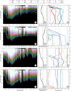 |
Fig. 4 Detailed atmospheric structures for a selected set of synthetic hot rocky exoplanets (ΨVMF =0, Mp =8 M⊕, Tirr =2500 K). Column 1: optical depth τ as function of wavelength and atmospheric pressure altitude. The photosphere, defined where the atmosphere has absorbed 50% of all incoming light, is indicated as solid white line; the 25% and 75% levels are shown in dotted white lines. Column 2: pressure–temperature structure. Column 3: speciation as function of pressure altitude. |
3.2.2 Variation with oxygen fugacity, volatile mass fraction, metallicity, and temperature
To further test the effect of the compositional parameters, we expanded our analysis to include ΔIW ∈ {−6, −3, 0, +3, +6}, ΨVMF ∈ {−1, 0, 1}, and varying Tirr ∈ {1000, 1500, 2500} K as shown in Fig. 5. We restrict the discussion to ξ ∈ {0, 1} (SOLAR vs. VIBSE), but we find that atmospheres with ξ ≥ 0.1 exhibit similar characteristics to the ξ =1 (VIBSE) cases.
In general, we find the volume-mixing ratios (VMRs) of major volatile species (e.g. CO, CO2, H2O, H2, He) to behave broadly similarly as in Fig. 4 for all cases investigated, meaning stable VMRs with altitude unless a thermal inversion induces dissociation of H2 and H2O. The tendency for atmospheres to undergo thermal inversions increases as Tirr increases, a result of the enhanced evaporation (and thus higher mixing ratios) of mineral species (cf. Zilinskas et al. 2023; Piette et al. 2023). Consequently, atmospheres formed around planets with Tirr < 2000 K show uniformly cooler upper atmospheres compared to their lower atmospheres that are subject to the greenhouse effect. As above, the proclivity for thermal inversion is greater at lower ξ (i.e. in SOLAR atmospheres) and lower ΨVMF, all else being equal, again owing to the higher mixing ratio of mineral gases that arises.
The pronounced greenhouse effect ensures that the vast majority of planets modelled show surface temperatures that exceed Tirr and in many cases cross the solidus of dry peridotite, ~1600 K (Katz et al. 2003). The extent of the greenhouse effect is relatively insensitive to ΔIW for VIBSE-like atmospheres, and translates into ΔT := TMAI − Tirr of ~800 K for Tirr =1000 K, ~600 K for Tirr =1500 K and roughly 300 K for Tirr = 2500 K. By contrast, the magnitude of ΔT for SOLAR cases is fO2 dependent and appears similar to VIBSE for oxidised cases, but decreases markedly for reduced cases, which can be attributed to the lack of effective greenhouse gases like CO2 (due to the high H/C ratio) or H2O (due to the low fO2) and the cooling effect of the inversion driven by the introduction of the anti-greenhouse gas SiO (see Sect. 3.2); similar results were found by Falco et al. (2024) for mixed H2-silicate atmospheres once the implicit shift in fO2 is accounted for. In VIBSE-like atmospheres (CO and CO2 rich) even an irradiation temperature of 1000 K might be sufficient to reach the required surface temperature for melting, while a reduced SOLAR-like atmosphere with a similar energy budget might be too cold to host a molten mantle (Fig. 5).
In systems with ΨVMF =1, the temperature at the bottom of the atmosphere suddenly declines below that of the isothermal radiative zone. This effect is most pronounced in SOLAR-like cases (Fig. 5) and results from a relative decrease in MIR opacity compared to the UVIS with increasing pressure. We note that this occurs at the upper limit of the tabulated values for the opacity (~1000 bar) and requires further investigation.
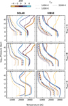 |
Fig. 5 Atmospheric thermal structure for representative scenarios. The pressure-temperature profiles for each simulated model is shown in colour, according to its oxygen fugacity, and the line style shows the Tirr of the model. Vertical grey lines indicate the irradiation temperature of the respective simulation. |
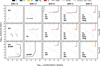 |
Fig. 6 Condensation degrees of elements (i.e. number fraction of an element that has condensed relative to its total atmospheric abundance) as function of atmospheric altitude for the Tirr =2500 K cases in the grid in Fig. 5. The colour denotes the element (red – Si, blue – Mg, teal – O, black – C, yellow – Fe), and the line style indicates the composition (solid – VIBSE; dashed – SOLAR). The pressure-temperature structure (at arbitrary units) is shown in light grey. The identity of condensates that occur in the respective atmospheres are SiC (silicon carbide), graph (graphite), fo (forsterite; Mg2SiO4), fa (fayalite; Fe2SiO4), qtz (quartz; SiO2), en (enstatite; MgSiO3), per (periclase; MgO), hem (hematite; Fe2O3), and mag (magnetite; Fe3O4). |
3.2.3 Condensation
The generally cooler upper atmospheric temperatures can, in many cases, induce partial condensation of the atmosphere. In Fig. 6, we show the condensation degrees of elements as function of altitude in the atmospheres from Fig. 5 for the Tirr = 2500 K case. The first striking observation is that, at this temperature, the SOLAR cases are nearly devoid of condensates (only for ΔIW+6, ΨVMF =−1, does forsterite condense), a consequence of the thermal structures of these atmospheres, which are typically inverted in the uppermost atmosphere (<10−4 bar) where condensation would otherwise occur.
Secondly, the nature of the condensing phases depend strongly on the fO2. Under highly reducing conditions (ΔIW-6), silicon carbide precipitates, sometimes alongside graphite when ΨVMF is high. However, the fraction condensed remains modest; only ~10% of the total element budgets of Si and C are removed from the gas. Further, the condensation of SiC occurs under high pressure (as high as several thousand bar), corresponding to the lower atmospheric layers; these regions generally lie beneath the photosphere (Fig. 4) and are thus hidden from observation. Graphite, on the other hand, may condense throughout the atmospheric column.
In neutral to oxidising atmospheres (ΔIW0 − ΔIW+3), the minerals forsterite (Mg2SiO4), enstatite (MgSiO3) and quartz (SiO2) condense. Iron condenses as fayalite (Fe2SiO4) in atmospheres initially equilibrated at ΔIW+3, while in highly oxidising systems (ΔIW ≥ +3), it can condense to form more oxidised phases, namely, hematite (Fe2O3) or magnetite (Fe3O4). Excess Mg not incorporated into forsterite can also condense as periclase (MgO) in the most oxidising atmospheres, while quartz is typically absent. In atmospheres with ΔIW ≳ 0, the condensation degree is high; nearly 100% of the Mg, Si and Fe is removed from the atmosphere. Unlike in the high ΨVMF, reduced atmospheres, condensation in oxidising atmospheres (ΔIW ≳ 0) occurs at lower pressures, where P ≲ 10−4 bar. Thus, the minerals have the potential to form high-altitude hazes, provided they do not settle.
For Tirr < 2500 K, the condensation front is pushed to lower altitudes in the atmosphere, and SOLAR-like atmospheres start condensing silicates in a similar manner to the VIBSE cases. Further, the condensation of carbon is expressed for all ΨVMF at ΔIW <0, either as SiC or graphite. However, the reduced vapour pressures of silicates at lower temperatures also decrease the total mass of condensates in the atmosphere, such that cooler atmospheres, despite greater condensation fractions, contain a lower mass of condensed phases.
3.3 Spectra
3.3.1 Emission
To investigate the effect of interior parameters on the emission spectrum, we follow the procedure outlined in Sect. 3.2 over a wider range of ξ ∈ {0, 0.1, 0.2, 0.5, 1}. The emission spectra are reported as the secondary eclipse depth (also called occultation depth or planet-to-star flux ratio):
![Mathematical equation: $\[\frac{F_p}{F_s}(\lambda)=\frac{\varepsilon_p(\lambda)}{\varepsilon_s(\lambda)} \cdot \frac{R_p^2(\lambda)}{R_s^2},\]$](/articles/aa/full_html/2026/06/aa57276-25/aa57276-25-eq16.png) (11)
(11)
where F is the totally emitted flux (erg s−2 cm−1), ϵ denotes the spectral exitance (erg s−2 cm−3), and R the radii of the respective bodies. The radius of the planet depends on the wavelength at which it is observed, as seen in the photospheres in Fig. 4. Assuming a constant radius does not produce inconsistencies when the atmosphere is highly compressed compared to the total radius (i.e. the VIBSE case, or a dry mineral atmosphere), but if it is extended, then Rp ≠ Rp,MAI, and wavelength dependence has to be incorporated; the method is highlighted in Appendix B.2. The resulting emission spectra are shown in Fig. 7 for Tirr = 2500 K, the average dayside temperature of 55 Cancri e that is consistent with phase curve observations (Demory et al. 2016a; Angelo & Hu 2017). Additional figures for lower Tirr are shown in Appendix H.
CO2 features are common among the studied archetypes. Distinct bands can be found in the mid-infrared at 2–3, 4.5 and 15 μm that similarly appear in almost all atmospheres where ΔIW ≥ 0. For ΔIW ≤ −3, these features either weaken or vanish, or, in the case of the 4.5 μm feature, blend with a CO absorption band of similar shape. Since the ratio pCO2/pCO depends on ![Mathematical equation: $\[f \mathrm{O}_{2}^{0.5}\]$](/articles/aa/full_html/2026/06/aa57276-25/aa57276-25-eq17.png) , and both gases have a similar opacity in this region, the 4.5 μm feature at a resolution accessible to the JWST Near Infrared Camera (NIRCam) has a similar depth for atmospheres of nearly all tested redox states and compositions except for the most reducing or metal-poor cases (ΔIW ≤ −3, ξ =0). Further, the 4.5 μm CO2 band also shows contribution from SO2 and CO, which deform the absorption trough at its blue and red ends, respectively (~4 μm and ~5 μm). In highly reduced, low-ξ or heavy ΨVMF =1 atmospheres (ΔIW =−6, ξ ≲ 0.1, ΨVMF =1), the 4.5 μm CO feature is converted from absorption into emission as the thermal structure of the atmosphere undergoes inversion (see Fig. 5). However, in turn, CO(g) emission merges with a SiO(g) emission feature at the same wavelength. The near-to-mid infrared CO2 wavebands at 2–3 μm also overlap with broad H2O features at 1–3 μm. Depending on the atmospheric composition, the dominant species will partially obscure the other; this effect is composition dependent. Similar to CO2, these water bands saturate at ΔIW ≳ −3, thus neither CO2 nor H2O features appear to be universal measurement devices for redox state. However, they can become indicative of highly reducing atmospheres (ΔIW < −3) if absent. The features that are sensitive to higher fO2 are the SO2 features at 8 and 21 μm (Hu et al. 2024; Nicholls et al. 2025b). They confidently indicate ΔIW ≳ 0 due to the dissolution of sulfur under reducing conditions (cf. Fig. 2). Both features manifest as absorption troughs whose intensity mirrors pSO2, and thus fO2, which shows a pronounced maximum at ΔIW+3 whereas any fO2 higher or lower produces a weaker signal. Additionally, fO2 exerts a significant influence on the baseline secondary eclipse depth, Fp/Fs, with variation of up to ~100 ppm for the planetary parameters over the 12 order-of-magnitude fO2 range explored here, caused by the conversion of (high-MMW) H2O into low-MMW H2, particularly affecting H-rich ξ =0 and ΨVMF =1 atmospheres, which leads to extended atmospheres and thus higher baselines (cf. Appendix B.2).
, and both gases have a similar opacity in this region, the 4.5 μm feature at a resolution accessible to the JWST Near Infrared Camera (NIRCam) has a similar depth for atmospheres of nearly all tested redox states and compositions except for the most reducing or metal-poor cases (ΔIW ≤ −3, ξ =0). Further, the 4.5 μm CO2 band also shows contribution from SO2 and CO, which deform the absorption trough at its blue and red ends, respectively (~4 μm and ~5 μm). In highly reduced, low-ξ or heavy ΨVMF =1 atmospheres (ΔIW =−6, ξ ≲ 0.1, ΨVMF =1), the 4.5 μm CO feature is converted from absorption into emission as the thermal structure of the atmosphere undergoes inversion (see Fig. 5). However, in turn, CO(g) emission merges with a SiO(g) emission feature at the same wavelength. The near-to-mid infrared CO2 wavebands at 2–3 μm also overlap with broad H2O features at 1–3 μm. Depending on the atmospheric composition, the dominant species will partially obscure the other; this effect is composition dependent. Similar to CO2, these water bands saturate at ΔIW ≳ −3, thus neither CO2 nor H2O features appear to be universal measurement devices for redox state. However, they can become indicative of highly reducing atmospheres (ΔIW < −3) if absent. The features that are sensitive to higher fO2 are the SO2 features at 8 and 21 μm (Hu et al. 2024; Nicholls et al. 2025b). They confidently indicate ΔIW ≳ 0 due to the dissolution of sulfur under reducing conditions (cf. Fig. 2). Both features manifest as absorption troughs whose intensity mirrors pSO2, and thus fO2, which shows a pronounced maximum at ΔIW+3 whereas any fO2 higher or lower produces a weaker signal. Additionally, fO2 exerts a significant influence on the baseline secondary eclipse depth, Fp/Fs, with variation of up to ~100 ppm for the planetary parameters over the 12 order-of-magnitude fO2 range explored here, caused by the conversion of (high-MMW) H2O into low-MMW H2, particularly affecting H-rich ξ =0 and ΨVMF =1 atmospheres, which leads to extended atmospheres and thus higher baselines (cf. Appendix B.2).
The influence of ξ is milder than that of fO2. Its principal effect is to lower the MMW as ξ decreases (cf. Fig. C.1), and thus extending the atmosphere, leading to slightly higher baseline secondary eclipse depths, Fp/Fs. Spectroscopically however, only the features of planets with ξ = 0 are visibly distinct from their higher-ξ peers, manifest as the weakening (at low ΨVMF) or disappearance (at high ΨVMF) of CO, CO2 and SO2 absorption in the 4.5, 8 and 15 μm bands, and the emergence of emission features of CO(g) and SiO(g) for ΔIW-6. In addition, the H2O bands in the near-to-mid infrared (~1–3 μm) trace ξ by means of their width and depth, however, remain generally more sensitive to ΨVMF (see below).
ΨVMF technically implies an accumulation of atmospheric mass, and thus, in principle, radial expansion. However, only the emission spectra of reduced or low ξ atmospheres seem to bear out this expectation (i.e., ΔIW ≤ −3 or ξ = 0), whereas the Fp/Fs of oxidised or high-ξ atmospheres maintain a similar shape and intensity as the total mass of atmosphere increases (Fig. 7). This occurs because their atmospheres are dominated by greenhouse gases whose opacities are so high that they become saturated at identical pressures, even at low ΨVMF. Specifically, even ΨVMF =−1 atmospheres have their photospheres at altitudes significantly above the surface. Any additional mass from larger ΨVMF accumulates below the photosphere, where they have effectively no spectroscopic expression. Due to the high compressibility of triatomic, high-MMW ideal gases (i.e. H2O, CO2 and SO2), the contribution to planetary radii is also negligible, and thus Fp/Fs remains near-constant despite increasing ΨVMF. The only exceptions are H2-rich atmospheres due to their low-MMW (cf. Sect. 3.3.2), which arises when fO2 and ξ are low (ΔIW ≤ −3 or ξ = 0); correspondingly, such atmospheres show a mild increase of the baseline Fp/Fs with increasing ΨVMF. In terms of spectroscopic changes, only the near-to-mid infrared (~1–3 μm) water bands continuously strengthen in depth and width as ΨVMF grows, from near absent at low ΨVMF to pronounced troughs at high ΨVMF, a result of greater H2O-abundance in high-ΨVMF atmospheres (Fig. 2).
Volatile rich atmospheres may still exhibit a SiO(g) feature in emission at 9 μm, akin to dry mineral atmospheres (Zilinskas et al. 2022; Piette et al. 2023; Falco et al. 2024; Seidler et al. 2024). The requirements for their emergence are low ΨVMF (i.e. low volatile masses, cf. Piette et al. 2023), reducing conditions (ΔIW ≲ − 3, Seidler et al. 2024) and SOLAR-like gas mixtures with ξ ~0. Earlier results by Zilinskas et al. (2023), using an out-gassing model in which mineral gas species and major volatile species are not in equilibrium (Falco et al. 2024), suggested that SiO features should disappear in the presence of hydrogen. Our results do not support such a general statement; some low-ξ atmospheres still show distinct SiO(g) features in emission, particularly at low ΨVMF (Fig. 7). Such emission features are only absent in carbon-rich atmospheres, as the opacities for CO(g) and CO2(g) are sufficiently high in the infrared (see Fig. D.1) so as to lead to upper atmospheric cooling, leading to the removal of mineral gases via condensation (see Sect. 3.2.3).
The generalities described above hold true for when Tirr < 2500 K, except that variation between redox regimes becomes increasingly non-linear with decreasing temperature (Figs. H.2, H.1), typified by sudden appearances of CO2 features at ΔIW-3 and SO2 at ΔIW+3, and the overall decline in Fp/Fs that makes detection more challenging (sensitivity of ΔFp/Fs ≪ 25 ppm required). Absorption features are also more readily observed, even in the most reducing cases, as thermal inversions, which would ordinarily be sustained by SiO(g), are not as marked, given the lower partial pressures of mineral gases and their tendency to condense; together, these processes lead first to a transition from SiO(g) emission to absorption features at Tirr =2000 K, and a complete disappearance of mineral gas features for Tirr =1500 K (Fig. H.1). Instead, methane absorption features unseen at higher temperatures appear in cold (Tirr ≤ 2000 K) and highly reduced atmospheres (ΔIW ≤ −3) (cf. Appendix J).
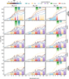 |
Fig. 7 Synthetic emission spectra over a grid in ΔIW ∈ {−6, −3, 0, +3, +6} (colour), ξ ∈ {0, 0.1, 0.2, 0.5, 1} (row) and ΨVMF ∈ {−1, 0, 1} (column). Other parameters were kept constant: Mp = 8M⊕, xmelt = 1 (fully molten mantle), Tirr =2500 K. Important broad-band spectral features are highlighted by coloured patches. The 4.5 μm feature, where multiple bands coalesce, is labelled 4.5r when reducing species (CO + SiO) dominate and 4.5o when oxidising species (CO2 + SO2) dominate. |
3.3.2 Transmission
In Fig. 8, we show the transmission spectra associated with the models presented in Sect. 3.3.1. Compared to the restricted range of secondary eclipse depths (~0–150 ppm), the transit depth varies by ΔRp ≳ 1 R⊕ between the models (with the bare-rock baseline being 1.7 R⊕), and thus we converted the usual transit depth
![Mathematical equation: $\[\delta=\left(\frac{R_p[\lambda]}{R_s}\right)^2\]$](/articles/aa/full_html/2026/06/aa57276-25/aa57276-25-eq18.png) (12)
(12)
into the (dimensionless) scaled density ρs for convenience:
![Mathematical equation: $\[\rho_s[\lambda]:=\frac{\rho_p[\lambda]}{\rho_{\oplus}(M_p)}=\frac{3 M_p}{4 \pi \delta^{3 / 2}[\lambda] \cdot R_s^3 \cdot \rho_{\oplus}(M_p)},\]$](/articles/aa/full_html/2026/06/aa57276-25/aa57276-25-eq19.png) (13)
(13)
where ρp is the planets (mean) density, ρ⊕(Mp) is the density of an upscaled Earth-like planet of mass Mp, and Rs is the radius of the star. Planets denser than Earth have ρs > 1 (likely corresponding to interiors dominated by a large iron-rich core), less dense objects have 0 < ρs < 1 (e.g. when the planet has an atmosphere). Since we assume here a constant Mp = 8 M⊕, ρs can be easily converted back to Rp.
The transit depth and thus ρs is coupled to the physical extent of the atmosphere, which can be approximated to the first order by its scale height, H:
![Mathematical equation: $\[H=\frac{R T}{\bar{m} \cdot g},\]$](/articles/aa/full_html/2026/06/aa57276-25/aa57276-25-eq20.png) (14)
(14)
where R is the gas constant, T is the temperature, ![Mathematical equation: $\[\bar{m}\]$](/articles/aa/full_html/2026/06/aa57276-25/aa57276-25-eq21.png) is the MMW of the gas, and g is the local gravitational acceleration (here, g = gMAI; note that this implicitly assumes the thin atmosphere approximation in which g is independent of altitude). The temperature profiles up to the photosphere are similar among models of equal Tirr, ΨVMF, and ξ (cf. Sect. 3.2), and therefore, the variation in ρs in Fig. 8 is mostly explained by variation in the MMW which ranges from 2 to 52 g/mol. This variation is driven primarily by ξ, with secondary sensitivity to fO2, and with a weaker dependence on ΨVMF (Fig. C.1). At constant ΨVMF and fO2, increasing ξ leads to high MMWs (
is the MMW of the gas, and g is the local gravitational acceleration (here, g = gMAI; note that this implicitly assumes the thin atmosphere approximation in which g is independent of altitude). The temperature profiles up to the photosphere are similar among models of equal Tirr, ΨVMF, and ξ (cf. Sect. 3.2), and therefore, the variation in ρs in Fig. 8 is mostly explained by variation in the MMW which ranges from 2 to 52 g/mol. This variation is driven primarily by ξ, with secondary sensitivity to fO2, and with a weaker dependence on ΨVMF (Fig. C.1). At constant ΨVMF and fO2, increasing ξ leads to high MMWs (![Mathematical equation: $\[\bar{m}\]$](/articles/aa/full_html/2026/06/aa57276-25/aa57276-25-eq22.png) ~ 28–44 g/mol) and thus more compact atmospheres as composition switches from H-dominated to C(±S) dominated. Low-ξ atmospheres are H2–He dominated and thus lighter (
~ 28–44 g/mol) and thus more compact atmospheres as composition switches from H-dominated to C(±S) dominated. Low-ξ atmospheres are H2–He dominated and thus lighter (![Mathematical equation: $\[\bar{m}\]$](/articles/aa/full_html/2026/06/aa57276-25/aa57276-25-eq23.png) ~ 2–5 g/mol), and thus significantly more extended. Consequently, they show lower scaled densities ρs, corresponding to greater transit radii. This effect is enhanced under reducing conditions and ΨVMF=1, both of which promote high pH2. However, despite the changes in bulk elemental chemistry with varying ξ at constant ΨVMF and fO2 (Fig. 1), we do not find major changes in the identity of C- and S-bearing absorbing species, nor in the relative strength of their features, a consequence of the relatively stable C/S ratio with ξ >0.1. Only H2O spectral bands are sensitive to ξ, as they increase in width as ξ becomes 0. Otherwise, ξ has only a minor influence on the shape of the transmission spectrum and instead chiefly governs the atmospheric extent. This implies a degeneracy with the radius of the condensed interior (Rp,MAI).
~ 2–5 g/mol), and thus significantly more extended. Consequently, they show lower scaled densities ρs, corresponding to greater transit radii. This effect is enhanced under reducing conditions and ΨVMF=1, both of which promote high pH2. However, despite the changes in bulk elemental chemistry with varying ξ at constant ΨVMF and fO2 (Fig. 1), we do not find major changes in the identity of C- and S-bearing absorbing species, nor in the relative strength of their features, a consequence of the relatively stable C/S ratio with ξ >0.1. Only H2O spectral bands are sensitive to ξ, as they increase in width as ξ becomes 0. Otherwise, ξ has only a minor influence on the shape of the transmission spectrum and instead chiefly governs the atmospheric extent. This implies a degeneracy with the radius of the condensed interior (Rp,MAI).
As in emission spectra, H2O and CO2 features are weak stand-alone indicators of fO2 due to their widespread appearance and similar strength across models with ΔIW ≳−3, including the 1–3 μm H2O bands and the 2–3, 4.5 and 15 μm CO2 bands. However, again similar to emission, the relative strength of the SO2 features becomes diagnostic of fO2. Alongside SO2, SO is also produced (see Sect. 3.1), exhibiting visible features between 0.3 and 0.4 μm and 0.8–1 μm in sulfur-bearing atmospheres. They also overlap with narrow but sharp, fO2-sensitive OH lines located between 300–400 nm (not resolved in Fig. 8). While pSO peaks near ΔIW+3 (similar to SO2), pOH continues to increase with fO2; distinguishing these features requires high resolution but can provide more stringent constraints on fO2. However, features of sulfur-bearing gases are preferentially associated with atmospheres of low transit depth and thus may be challenging to observe. High-resolution ground-based spectroscopy could access both SO and OH features in the UVIS in addition to the nearby water bands at ~1 μm, but feasibility remains to be tested.
Mineral gases also appear in transmission spectra, and most prominently in the UV (λ ≤ 300 nm) in the form of an intense SiO feature. Lines of Mg, MgO and Fe also occur in the UVIS, respectively at ~285 nm, 500 nm and 300–600 nm. These spectral lines overlap with those of the aforementioned SO, OH and H2O-bearing waveband, providing complementary fO2 indicators that are sensitive to changes below ΔIW < 0 (unlike the aforementioned SO2, H2O and CO2). At longer wavelengths (9 μm), SiO has additional features that are clearly visible in very reduced (ΔIW ≤ −3) atmospheres of any ξ and ΨVMF ≤ 0, and define viable targets for space-based transmission spectroscopy, for example with JWSTs Mid Infrared Instrument (MIRI), or ground based high-resolution spectroscopy (Dash et al. 2025). If the partial pressures of mineral gases are high (i.e. under highly reducing conditions and high temperatures), they increase ![Mathematical equation: $\[\bar{m}\]$](/articles/aa/full_html/2026/06/aa57276-25/aa57276-25-eq24.png) of the H-He-dominated background gas, leading to lower transit depths. This effect is evident in low-ξ, low-ΨVMF atmospheres, where the most reduced models are not the most extended ones.
of the H-He-dominated background gas, leading to lower transit depths. This effect is evident in low-ξ, low-ΨVMF atmospheres, where the most reduced models are not the most extended ones.
As in emission spectroscopy, ΨVMF exerts a limited effect on the extent of the atmosphere for the same reasons (cf. Sect. 3.3.1). Thus, atmospheres with varying ΨVMF ∈ {−1, 0} appear similar in transmission spectra when ξ and fO2 are held constant, especially in oxidised, high-ξ cases, and only scale with ΨVMF if the atmosphere is highly enriched in H2 and He (i.e. ξ =0 or ΨVMF =1 at ΔIW ≤ −3). High-ΨVMF atmospheres have more pronounced water bands that scale with ΨVMF (as per emission spectra) and could, especially in comparison with the CO2 band at 4.5 μm, place constraints on the total atmospheric pressure. Additionally, enhancement of the aforementioned SO(g)+OH(g) absorption bands between 300–400 nm with increasing ΨVMF is observed. Combined observation of these features might reveal the ΨVMF. However, similar to ξ, the change in base-line induced by this parameter is expected to be degenerate with Rp,MAI.
Finally, the prominent CH4 and HCN features that appear in the NIR and MIR for reduced, high-ΨVMF atmospheres may not be realistic, as the abundance of acetylene is so high that it may start dominating the opacity. However, its spectral line list remains incomplete, and the models presented herein have to be interpreted with caution (see Sect. 4.4 and Appendix J).
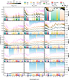 |
Fig. 8 Transmission spectra of the synthetic atmospheres from Fig. 7 rearranged to highlight the effect of ξ, which was (nearly) absent in emission. The spectra are reported in terms of the scaled density, Eq. (13), which at constant mass (here, Mp = 8M⊕) can be directly related to the radius (right axis). Prominent spectral features are highlighted by coloured bands. |
4 Discussion
4.1 Comparison to mass-radius measurements
Since our model predicts the radius of a planet, it can be used to provide first-order estimates on the required atmospheric properties of observed HREs given their measured mass and radius. We therefore selected planets with periods <4 days from the NASA Exoplanet Archive9 and show them in a mass-density diagram (Fig. 9), in which the scaled density ρs (Eq. (13)) is plotted. The radius, needed to compute ρs, was averaged over the Kepler bandpass (400–900 nm). Overlain on the observational data are synthetic mass-density curves for a SOLAR and VIBSE composition, evaluated at reducing (ΔIW-3) and oxidising (ΔIW+3) conditions and for two temperatures, Tirr =1250 K and Tirr = 2500 K to mirror the range of HREs. Note that in this context, Tirr is equal to the average dayside temperature, corresponding to a dilution factor of 𝔣 = 2/3 (Hansen 2008), motivated by the findings of Hammond & Pierrehumbert (2017) and Zhang & Showman (2017) that the hot-spots of high-MMW atmospheres remain confined to the dayside. ΨVMF = 0 was held constant, but its effect on ρs can be inferred from Fig. 8.
We identify a population of under-dense planets with ρs < 0.5, all of which lie to the left of the M − ρs curves defined by the SOLAR-composition lines (dotted and dash dotted lines). Prominent examples are TOI-1408 c, TOI-544 b and HD 110131 b. This marks these objects as likely metal-poor, as greater atmospheric extent is found in low-ξ atmospheres (Sect. 3.3.2); high-ξ atmospheres reach such low ρs only when they are massive (ΨVMF =1) and highly reducing (ΔIW ~ − 6; see Fig. 8), such that most sulfur and nitrogen has dissolved and carbon has been sequestered from the gas phase via graphite formation (cf. Fig. 2). These planets might be likened to gas dwarfs if reducing (e.g. Mol Lous et al. 2024) or waterworlds if oxidising (e.g. Dorn & Lichtenberg 2021). TOI-1408 c stands out due to its Tirr of ~2500 K, Mp ~ 7.6 M⊕ and Sun-like host star, which makes the planet similar to 55 Cnc e and thus comparable to the simulations from Sect. 3.3. In Fig. 10, we compare the modelled to the observed ρs for TOI-1408 c and 55 Cnc e. For TOI-1408 c, only solutions with ΨVMF ≥ 0 fit the observed ρs, with the degree of ξ enrichment being tied to fO2 and favouring C–N–S-poor, reducing solutions. Intermediate to oxidised scenarios (ΔIW ≥ 0) akin to a waterworld scenario remain possible within 2 σ. The higher Tirr and the accompanying atmospheric size increase implies that TOI-1408 c requires less volatile material compared to typical sub-Neptunes to explain its low density. Thus, it may bear strong signatures of mineral gases, particularly SiO at 9 μm, if it sustains a magma ocean below its atmosphere (Sect. 3.3.2). However, our assessment hinges on the assumption of 𝔣 = 2/3. Heat redistribution in low-MMW atmospheres may cause the dayside temperature to approach the equilibrium temperature instead (Hammond & Pierrehumbert 2017), which would imply we may overestimate atmospheric extent (Eq. (14)) and thus underestimate the volatile content. It also stands to mention that planets in this category are highly inflated and H-He rich, which could leave them vulnerable to (rapid) atmospheric loss (e.g. Salz et al. 2016; Bourrier et al. 2018). If primarily H–He are lost, ξ and fO2 may increase (cf. Cherubim et al. 2025).
A population of intermediate density HREs plots in between the M–ρs trends set by the SOLAR and VIBSE endmembers (0.6 < ρ/ρ⊕ < 0.8). This indicates a substantial atmosphere, whose nature is not defined from mass-density considerations alone. Examples of HREs that might adhere to this category are 55 Cnc e10, TOI-561 b and TOI-1416 b. To first order, the reduced, SOLAR-like case (dotted lines) and the oxidised VIBSE-like case (solid lines) are poor fits for planets in this category, as they would be too extended or compressed, respectively, even under varying ΨVMF (see Fig. 8). Their compositions are thus more likely to lie intermediate to SOLAR and VIBSE (ξ ~0.2–0.5), and to be degenerate with fO2 such that higher-ξ solutions only fit when they are reduced (H2–atmospheres enriched in either CO + SiO when ΨVMF =−1 or CO+hydrocarbons when ΨVMF ≥ 0; see Appendix J), while oxidised cases are only consistent with their radii when ξ is low (H2O-rich). This is demonstrated in detail for 55 Cnc e in Fig. 10. As ρs scales predictably with mass when Mp > 2 M⊕ (Fig. 9), similar conclusions hold for all planets with ρs ~ 0.6–0.8.
Planets of even higher scaled density (0.8 < ρ/ρ⊕ < 0.9) are best approximated by the VIBSE cases, either reduced (CO-dominated) or oxidised (CO2–SO2 dominated). Technically, their densities are sufficiently high that an atmosphere is not strictly required (within uncertainty), but the interior would be required to be coreless (CORL; dashed light-blue line in Fig. 9) (Elkins-Tanton & Seager 2008). Falling into this category are WASP-47 e (according to updates in its mass-radius measurements from transit-timing variations, Nascimbeni et al. 2023) and Kepler-10 b.
Planets that fall closer to the ρs = 1 line are consistent with a rocky interior similar to Earth’s. However, the average uncertainties are typically too large to firmly distinguish such a planet from atmosphere-bearing cases, as exemplified by HD 213885 b. Some planets, notably K2-141 b, TOI-431 b and CoRoT-7 b, plot to even higher scaled densities (ρ/ρ⊕ > 1.0), which implies an interior structure with a higher core-mantle ratio than Earth (e.g. Adibekyan et al. 2021). However, this does not preclude the existence of an atmosphere, as the density decrease induced by an atmosphere could be offset by an even larger core. Even if no volatile-rich atmosphere is present, the planets might still possess a pure mineral gas atmosphere that is highly compressed and confined to the dayside, therefore having no resolvable impact on the radius (Seidler et al. 2024).
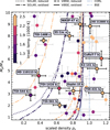 |
Fig. 9 Mass versus the scaled density for observed (dots) and modelled planets (lines). Scaled density is defined as ρ/ρ⊕, where ρ⊕(M) is the density of a planet with the same interior structure and composition as Earth at a given mass (M). The radii of the modelled planets are based on the radius of the photosphere, which was averaged over the Kepler bandpass. The curves for atmosphere-bearing planets are computed for endmember cases (ξ = VIBSE, SOLAR; ΔIW = −3, +3; Tirr = 1250 K, 2500 K, at constant ΨVMF =0). Curves for two atmosphere-free cases (a coreless planet; CORL and a BSE-like planet, BSE) are also shown. The points denote a collection of measured masses and radii for planets R ≤ 4 R⊕, M ≤ 10 M⊕ and Tirr ≥ 1000 K, obtained from the NASA Exoplanet Archive; we omit objects with an uncertainty σρscaled > 0.25 from the plot. |
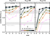 |
Fig. 10 Average scaled density of the synthetic models from Fig. 8 in the Kepler/TESS bandpass (400–900 nm), shown as a function of ΔIW and ΨVMF (coloured lines and dots). The colour corresponds to ξ. The simulations are compared to the inferred scaled densities for 55 Cancri e and TOI-1408 c, which are shown as grey bands; their width denotes the 1σ limit. The dashed black line indicates the scaled density of an atmosphere-free (airless) planet, i.e. Rp,MAI (Sect. 2.1.1). |
4.2 Spectral constraints on the atmosphere of 55 Cancri e
Recently, JWST observations of 55 Cnc e were published (Hu et al. 2024; Patel et al. 2024). The MIRI data presented by Hu et al. (2024) (black points; Fig. 11) record a constant Fp/Fs near ~100 ppm, cited as evidence of an atmosphere owing to the suppression of the flux contrast relative to bare rock. This atmosphere might also be reducing, given that the flat spectrum rules out an intense SO2 feature (cf. Sect. 3.3.1). In our study, we further support this conclusion. The intensity predicted in this segment of the emission spectrum for models with visible SO2 features (VIBSE, ΔIW+3) is ~2σ lower than the observed Fp/Fs, even ruling out the scenario of an Earth-like, reduced (i.e. CO-bearing) atmosphere found by Hu et al. (2024). Instead, the MIRI observation can be fit by a degenerate set of solutions that include highly reduced (ΔIW-6) CO-rich compositions at low to moderate ΨVMF (−1 and 0) and moderate- to high-ξ (0.1 to 1), to comparatively oxidised (ΔIW ≥ 0), ΨVMF = 0 H2O-rich planets. The best fit scenario from our discrete model grid, based on a χ2 estimate, is an atmosphere with ΨVMF = 0, ξ = 0.5 and ΔIW-6 (black curve in Fig. 11) which is also consistent with the radius constraints (Sect. 4.1). In addition to the VIBSE cases, massive (high ΨVMF), reduced SOLAR-like cases (gas dwarfs) can be excluded, supporting the notion that this planet is neither a more massive Earth analogue, nor is it a planet that captured and maintained a primordial atmosphere. A similar degeneracy, with pure CO or H2O atmospheres fitting the MIRI observations, was also found by Zilinskas et al. (2025).
In terms of the NIRCam observations by Hu et al. (2024) and Patel et al. (2024), no clear trend can be deduced. Any attempt at fitting the observations, either individually or combined, was stifled by the variability of the target (Patel et al. 2024) and the strong auto-correlation within the derived white light curves that does not allow for the deduction of the absolute flux value (cf. Hu et al. 2024; Patel et al. 2024; Zilinskas et al. 2025). The currently available data are thus unlikely to yield robust constraints, and further investigation is required to alleviate these shortcomings.
Besides JWST, 55 Cnc e has been the target of multiple missions. Of interest to our study are the observations by Esteves et al. (2017) and Jindal et al. (2020), which limits the combinations of ![Mathematical equation: $\[\bar{m}\]$](/articles/aa/full_html/2026/06/aa57276-25/aa57276-25-eq25.png) and H2O–VMR, potentially ruling out cases of ξ ≲ 0.1 and dIW>0. Deibert et al. (2021) rule out the most reduced “acetylene world” scenarios (Appendix J) based on the non-detection of C2H2 and HCN at low
and H2O–VMR, potentially ruling out cases of ξ ≲ 0.1 and dIW>0. Deibert et al. (2021) rule out the most reduced “acetylene world” scenarios (Appendix J) based on the non-detection of C2H2 and HCN at low ![Mathematical equation: $\[\bar{m}\]$](/articles/aa/full_html/2026/06/aa57276-25/aa57276-25-eq26.png) ; slightly more oxidising scenarios (ΔIW-3) remain possible. Tsiaras et al. (2016) however found hints for a HCN-bearing, H2-rich atmosphere. Ehrenreich et al. (2012) and Zhang et al. (2021) on the other hand fail to detect escaping H and He, respectively, an observation possibly at odds with the apparent ξ < 1 of our proposed cases for 55 Cnc e. However, the hot-spot shift seen with Spitzer (Demory et al. 2016a; Angelo & Hu 2017) in conjunction with the atmospheric circulation models from Hammond & Pierrehumbert (2017); Zhang & Showman (2017) again lend support to an H-bearing, low-
; slightly more oxidising scenarios (ΔIW-3) remain possible. Tsiaras et al. (2016) however found hints for a HCN-bearing, H2-rich atmosphere. Ehrenreich et al. (2012) and Zhang et al. (2021) on the other hand fail to detect escaping H and He, respectively, an observation possibly at odds with the apparent ξ < 1 of our proposed cases for 55 Cnc e. However, the hot-spot shift seen with Spitzer (Demory et al. 2016a; Angelo & Hu 2017) in conjunction with the atmospheric circulation models from Hammond & Pierrehumbert (2017); Zhang & Showman (2017) again lend support to an H-bearing, low-![Mathematical equation: $\[\bar{m}\]$](/articles/aa/full_html/2026/06/aa57276-25/aa57276-25-eq27.png) atmosphere consistent with the best-fit cases in Fig. 11. Finally, high-resolution spectroscopy has not recovered Fe(g) in emission (Rasmussen et al. 2023), and found no evidence of an extended Fe–Mg-bearing atmosphere in transmission (Keles et al. 2022). This could potentially exclude clear, low-density, low-ξ models from Fig. 8 that show such lines at ~0.5 μm; however, the direct comparability of our models to the template spectra used in their studies remains uncertain, as they were volatile free and probed a limited selection of silicate vapour compositions.
atmosphere consistent with the best-fit cases in Fig. 11. Finally, high-resolution spectroscopy has not recovered Fe(g) in emission (Rasmussen et al. 2023), and found no evidence of an extended Fe–Mg-bearing atmosphere in transmission (Keles et al. 2022). This could potentially exclude clear, low-density, low-ξ models from Fig. 8 that show such lines at ~0.5 μm; however, the direct comparability of our models to the template spectra used in their studies remains uncertain, as they were volatile free and probed a limited selection of silicate vapour compositions.
In summary, current spectral observations provide only indirect and contradictory evidence of the presence and composition of an atmosphere on 55 Cnc e. Whether the apparent inconsistencies between observations and models arise primarily from observational challenges or from simplifying assumptions in atmospheric modelling remains unclear. Some major limitations of our approach are discussed in Sect. 4.4.
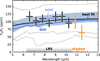 |
Fig. 11 Observations from MIRI of 55 Cancri e (black markers, Hu et al. 2024), including the MIRI shadow region (orange markers), compared to a selection of synthetic emission spectra (coloured and grey lines). The blue shaded area indicates the range of spectra that matches the observation, based on a χ2-fit (excluding the shadow region). Three endmembers within the set of matching models are highlighted: the best fit (black, ΨVMF = 0, ΔIW-6 and ξ = 0.5), a mineral-rich He–H2–CO–SiO–atmosphere (minC, bright blue, ΨVMF = −1, ΔIW-6 and ξ = 0.1), and a waterworld (WW, dark blue, ΨVMF = 1, ΔIW+6 and ξ = 0). Relevant non-fitting models are shown in grey and comprise the gas-dwarf scenario (GDw, ΨVMF = 1, ΔIW-6 and ξ =0) as well as a reduced (rBSE, ΨVMF = 0, ΔIW-3 and ξ =1) and an oxidised VIBSE scenario (oBSE, ΨVMF = 0, ΔIW+3 and ξ = 1). |
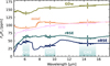 |
Fig. 12 Prediction for MIRI MRS MEDIUM channel observations of 55 Cancri e for selected synthetic atmospheric models (identical to Fig. 11). Uncertainties were simulated via the pandeia.engine package (v4.0) (Exposure Time Calculator, ETC, Pontoppidan et al. 2016) with JWST reference data (Space Telescope Science Institute 2024), assuming 7 groups and 19.4 seconds per exposure. Only channels 1, 2 and 3 are shown (CH1-CH3); channel 4 at 25 μm is unlikely to yield useful constraints owing to its low through-put. |
4.3 Future observations
In Fig. 12, we show five distinct scenarios for the atmosphere of 55 Cancri e, together with predicted measurements using the MIRI medium resolution spectroscopy (MRS) mode. In contrast to the low-resolution (LRS) mode used by Hu et al. (2024), the detector does not saturate, in spite of the star’s brightness, and can thus be used to retrieve robust results. The MRS mode offers four different channels with three subbands (SHORT, MEDIUM, and LONG) each. To capture important features (CO2 at 15 μm, SO2 and SiO at 9 μm), the medium channel is required. It becomes apparent that the predicted observations – when the spectrum in each channel is binned over the whole bandpass – is sufficient to distinguish between the endmember scenarios of gas dwarfs with primordial atmospheres (ΨVMF = 1, ΔIW-6, ξ =0), steam planets (ΨVMF = 1, ΔIW0, ξ = 0), VIBSE-like planets and their redox states (ΨVMF = 0, ΔIW-3 (reduced) /ΔIW+3 (oxidised), ξ =1) and mineral gas enriched atmospheres (ΨVMF =−1, ΔIW-6, ξ = 0). A future observation of 55 Cancri e was approved in Cycle 4 GO, proposal 7875, Zhang et al. 2025. However, it must be noted that a significant degree of information hinges on the baseline of the secondary eclipse flux, and any inference will be degenerate with the size of the condensed interior (Sect. 4.1) and the heat redistribution of the atmosphere (Zilinskas et al. 2025). This information can be constrained by obtaining phase curves (which constrain the heat redistribution) and the primary transit, which determines the size of the atmosphere (Sect. 3.3.2).
4.4 Limitations and improvements
Due to limitations in theory, observation, and experimental data, a number of simplifying assumptions had to be made. Below we list the ones we consider the most impactful on our results.
Incomplete or missing line lists represent a major limitation of this study. Some species occur in appreciable abundances in HRE atmospheres, yet lack short-wave opacities, for example acetylene (C2H2) and methane (CH4). Both gases occur exclusively under highly reducing conditions (ΔIW ≲−3), with the latter emerging only in cooler atmospheres (Tirr ≲ 2000 K). Acetylene may, however, become a dominant absorber in massive atmospheres (ΨVMF ≥1), but opacity data below 1 μm are missing (Fig. D.1), meaning its inclusion would result in a spurious greenhouse effect (see Appendix J). Complete opacities of important species in massive, reduced atmospheres is required. To eliminate these biases, the available line lists have to be extended via experimental and theoretical means, and evaluated over the whole pressure-temperature range of HRE atmospheres.
The solubility laws used in this work are described according to Henry’s or Sieverts’ law approximations, which may break down when the concentration of the solute increases, and pressures, temperatures and fO2 diverge from those at which the laws were calibrated (see Table A.1 or Bower et al. 2025, their Table 1). This is particularly relevant for the hotter HREs, for which surface temperatures can approach 3000 K. By contrast, experimental constraints are typically half that temperature; only H2O was measured to applicable temperatures (~2173 K, Sossi et al. 2023). Further, the Henry’s law constants for all species except H2O (Sossi et al. 2020) were obtained for basaltic or andesitic compositions of the melt, which, though reasonable approximations, are unlikely to hold for magma oceans on exoplanets. This may pose problems for species with composition-dependent solubilities, like S2 (which is a complex function of melt FeO content, O’Neill & Mavrogenes 2002; Boulliung & Wood 2023) or H2, N2 and the noble gases that dissolve by physical incorporation (Carroll & Draper 1994). Furthermore, all solubility laws are derived for either pure gases or simple mixtures thereof, and thus the true solubilities may deviate from those reported in this study. More experimental measurements have to be obtained.
All the radiative transfer codes used here (HELIOS and petitRADTRANS) as well as FastChem assume an ideal gas equation of state, which is violated by heavy atmospheres (≳1000 bar). This issue is fundamental and goes beyond the scope of this study (cf. Sect. 2.1.2), but only affects the layers below the photosphere (Pphoto ≲ 1 bar in all cases). Likely implications are (i) miscalculation of atmospheric elemental ratios (e.g. C/O), (ii) underestimation of dissolved content (since fugacity coefficients for major volatiles tend to exceed 1 at high pressures), (iii) differences in speciation in the atmospheric column of the lower atmosphere (as computed by FastChem), and (iv) an underestimation of the planets radius, as non-ideal species of the major volatiles are less compressible than ideal gases (Holland & Powell 1991; Shi & Saxena 1992; Bower et al. 2025). Issues (i) and (ii) can in principle be corrected for by passing a non-ideal equation of state to Atmodeller. Issues (iii) and (iv) cannot be mended without major adaptions to the other underlying codes.
While we included the effect of condensation on the removal of a gas phase, we did not include the formation of clouds or hazes. In a realistic HRE atmosphere with eddy diffusion and strong day-nightside thermal gradients (Hammond & Pierrehumbert 2017; Zhang & Showman 2017), condensation may occur as gas is advected to cooler upper layers or the nightside (cf. Nguyen et al. 2024). If present, clouds may substantially alter transmission spectra, potentially impeding observability of key spectral features (Janssen et al. 2026). However, more detailed studies on the influence of condensation on P–T-structure and spectra in both 1D and 2D/3D models are required.
The heat redistribution factor 𝔣 might deviate in the presence of strong day-to-nightside advection from the herein assumed value of 2/3. It exerts a strong influence on the secondary eclipse spectra, with smaller 𝔣 lowering the simulated emission flux of 55 Cnce by ~20–50 ppm when changing 𝔣 from 2/3 (Tirr =2500 K, average dayside temperature) to 1/4 (Tirr = 2000 K, equilibrium temperature). This difference is crucial to consider when fitting the observed spectra, as they result in divergent best-fitting models (Zilinskas et al. 2025). To constrain 𝔣, multi-wavelength full phase curve observations are required.
All preceding analysis was made under the assumption of a fully molten Earth-like interior structure and a restricted set of bulk volatile compositions. Deviations therefrom (e.g. changes in CMF, mantle and core composition, mantle melt fraction, or volatile compositions deviating from the mixing line defined by ξ) may result in significant changes to Rp and transmission and emission spectra. However, the necessary changes in the interior structure would indicate that the outliers found in Sect. 4.1, including 55 Cnc e, TOI-1408c and TOI-561 b, would have to deviate from the upscaled Earth-like scenario regardless. The diversity in HRE composition and interior structure thus appears robust, but its details remain to be studied in more extensive work.
5 Summary and conclusions
Despite varying bulk chemistry, volatile-rich mineral gas atmospheres are generally dominated by He, CO, CO2, H2, and H2O. The fO2 controls the ratios of CO/CO2 and H2/H2O, where CO and H2 are favoured in reducing atmospheres and CO2 and H2O in oxidising atmospheres. The pSO2 reaches a maximum near ΔIW+3, owing to its dissolution as S2− at lower fO2 and ![Mathematical equation: $\[\mathrm{SO}_{4}^{2-}\]$](/articles/aa/full_html/2026/06/aa57276-25/aa57276-25-eq28.png) at higher fO2, rendering it the dominant gas in oxidising highξ atmospheres. H2O as the prevailing gas only occurs in heavy low-ξ atmospheres due to its high solubility, while He, when present, resides almost exclusively in the atmosphere, as do CO and CO2. Nitrogen is also insoluble (as N2) except at low fO2, at which point N3− is stable in the melt. Mineral gases, such as SiO, Mg, MgO, and Fe evaporate preferentially in highly reduced (ΔIW ≲ −3) and hot atmospheres (Tirr ≳ 2000 K). Cooler, higher ΨVMF and reducing atmospheres (T < 2000 K) are more prone to form methane instead of CO, with the occurrence of CH4, C2H2, and HCN. In reduced atmospheres at the highest temperatures and ΨVMF, SiH4 becomes abundant, but the ideal gas approximation is no longer valid in such cases.
at higher fO2, rendering it the dominant gas in oxidising highξ atmospheres. H2O as the prevailing gas only occurs in heavy low-ξ atmospheres due to its high solubility, while He, when present, resides almost exclusively in the atmosphere, as do CO and CO2. Nitrogen is also insoluble (as N2) except at low fO2, at which point N3− is stable in the melt. Mineral gases, such as SiO, Mg, MgO, and Fe evaporate preferentially in highly reduced (ΔIW ≲ −3) and hot atmospheres (Tirr ≳ 2000 K). Cooler, higher ΨVMF and reducing atmospheres (T < 2000 K) are more prone to form methane instead of CO, with the occurrence of CH4, C2H2, and HCN. In reduced atmospheres at the highest temperatures and ΨVMF, SiH4 becomes abundant, but the ideal gas approximation is no longer valid in such cases.
The atmospheric structures of HREs are typified by strong greenhouse effects in the lower atmosphere, induced by CO, CO2, H2O, and SO2, which is nearly universally present but exacerbated in oxidised atmospheres (ΔIW ≳0). In these cases, the surface of the planet is up to 800 K hotter than its irradiation temperature, which allows for magma oceans on planets with irradiation temperatures as low as 1000 K. The same gases cause cooling in the upper atmosphere, decreasing the upper atmospheric temperature by up to 1500 K compared to the irradiation temperature. On the other hand, an upper atmosphere thermal inversion appears in atmospheres whose opacity structure is dominated by mineral gases, mainly SiO, which is the case in reduced and hot systems of low ΨVMF.
Secondary eclipse depths are mostly sensitive to temperature and oxygen fugacity (fO2) and to a lower degree to metallicity (ξ) and the volatile content (ΨVMF). Key molecules with strong absorption features include SO2, CO2, and H2O. When the atmosphere is inverted, CO and SiO appear as emission features. SO2 is the most robust tracer of fO2 in the range ΔIW +3±3, except at ξ ~0, where the feature appears weak due to low total sulfur abundances. CO2 and H2O are present across a wide range of conditions, making them poor stand-alone redox indicators, but they allow for constraints on metallicity (ξ) and volatile amounts (ΨVMF). SiO emission at 9 μm identifies hot, highly reducing low-metallicity atmospheres. Cooler (Tirr ≲ 2000 K) and highly reduced atmospheres might show CH4 features instead, which may be replaced by C2H2 features in a more realistic setting. The 4.5 μm region (JWST NIRCam) is spectrally degenerate in CO2, CO, SO2, and SiO, while the JWST MIRI instrument can distinguish between redox regimes and temperatures by targeting distinct CO2, SO2, and SiO features in the 7–20 μm band.
The transit depth is mainly governed by ξ: low-ξ atmospheres are significantly more extended than their compressed high-ξ counterparts. However, the identity and shape of spectral features in transmission is still dictated by fO2, and they show ξ-sensitive H2O and redox-sensitive SO2 features in the mid-infrared to the same effect as emission spectra. H2O bands between 1–2 μm also become tracers of atmospheric mass (ΨVMF) for oxidised low-ξ atmospheres, while planets with ξ ~ 0 show strong mid-IR SiO and CO features. The UVIS to NIR (300–1000 nm) shows a minimum in transit depth but hosts lines from SO, OH, Fe, Mg, MgO, SiO, and H2O that vary with fO2, offering a promising window for ground-based detection of magma oceans and retrievals of the fO2.
In the cooler upper layers, condensation of silicates, oxides, and carbides might occur. In ξ = 0 atmospheres, condensation is suppressed by the thermal inversion; in oxidised high-ξ atmospheres, condensation of silicates (and oxides at the highest fO2) occurs in the upper atmospheric layers despite irradiation temperatures of 2500 K due to the cooling effect of the greenhouse gases. Reduced high-ξ planets condense SiC in their lower to middle atmosphere, and graphite at nearly all altitudes. Tirr < 2000 K progressively leads to condensation at greater atmospheric depths, and condensation in lower-ξ atmospheres.
While the majority of mass-radius relationships of the hottest HREs are consistent with atmospheres with a limited scale height (favoured at high ξ), some, such as 55 Cancri e and TOI-1408 c, have densities that are too low to be explicable by a bulk silicate Earth-like volatile budget (i.e. ξ =1 and ΨVMF =0). Hence, these HREs are consistent with intermediate ξ ~ 0.1–0.5 atmospheres in the case of 55 Cancri e or, in the case of TOI-1408 c, favour SOLAR-like (ξ =0), massive (ΨVMF =1), and highly reducing (ΔIW ≲−3) scenarios to explain their extended atmospheres. We find that mass–radius relations are degenerate with respect to ξ and ΨVMF, which can only be resolved by spectroscopic means.
The MIRI spectra of 55 Cancri e obtained by Hu et al. (2024) preclude VIBSE-scenarios at any ΨVMF and any ΔIW ≥ −3, as well as highly reduced (ΔIW-6) SOLAR cases at ΨVMF ≥ 1, indicating that the planet is neither a heavier Earth-twin nor that it captured an extensive nebular atmosphere. Intermediate scenarios remain possible. This conclusion aligns with the constraints from the mass-radius data at a shorter wavelength. The NIRCam observations by Hu et al. (2024) and Patel et al. (2024) do not paint a consistent picture and remain inconclusive. Ground-based observations might disfavour H-rich (low-ξ) scenarios. Future observations with MIRI’s MRS mode can place constraints on the possible scenarios but will remain degenerate with the interior structure and the temperature distribution of the planet.
Data availability
The MAGMA code can be obtained from Bruce Fegley Jr. upon reasonable request. The other codes used in this study are distributed under permissive software licences and can be obtained from the respective sources (see below). The scripts used to produce this study can be found on github (https://github.com/ExPlanetology/volbear-scripts), and the data products can be found on zenodo (https://zenodo.org/records/19571079). This work made use of the following codes: Atmodeller v1.0.0 (Bower et al. 2025), phaethon (Seidler et al. 2024), HELIOS (Malik et al. 2017, 2019), FastChem (Kitzmann et al. 2024), MAGMA (Fegley Jr & Cameron 1987; Schaefer & Fegley Jr 2004), numpy (Harris et al. 2020), scipy (Virtanen et al. 2020), pandas (Wes McKinney 2010), matplotlib (Hunter 2007), seaborn (Waskom 2021), astropy (Astropy Collaboration 2013, 2018, 2022), bayes_opt (Nogueira 2014).
Acknowledgements
We thank Merlin Zgraggen and Lukas Felix for their collaboration on an unaccepted JWST proposal; from their contribution, we deduced the uncertainties in the expected MRS observation shown in Fig. 12. This work was supported by the Swiss National Science Foundation (SNSF) through an Eccellenza Professorship (203668) and the Swiss State Secretariat for Education, Research and Innovation (SERI) under contract No. MB22.00033, a SERI-funded ERC Starting grant “2ATMO” to P.A.S. Parts of this work have been carried out within the framework of the National Centre of Competence in Research (NCCR) PlanetS supported by the SNSF under grant 51NF40_205606. This publication makes use of The Data & Analysis Center for Exoplanets (DACE), which is a facility based at the University of Geneva (CH) dedicated to extrasolar planets data visualisation, exchange and analysis. DACE is a platform of the Swiss NCCR PlanetS, federating Swiss expertise in Exoplanet research. The DACE platform is available at https://dace.unige.ch.
References
- Abel, M., Frommhold, L., Li, X., & Hunt, K. L. 2011, J. Phys. Chem. A, 115, 6805 [NASA ADS] [CrossRef] [Google Scholar]
- Abel, M., Frommhold, L., Li, X., & Hunt, K. L. 2012, J. Chem. Phys., 136, 044319 [NASA ADS] [CrossRef] [Google Scholar]
- Adibekyan, V., Dorn, C., Sousa, S. G., et al. 2021, Science, 374, 330 [NASA ADS] [CrossRef] [Google Scholar]
- Aguichine, A., Mousis, O., Deleuil, M., & Marcq, E. 2021, ApJ, 914, 84 [NASA ADS] [CrossRef] [Google Scholar]
- Amundsen, D. S., Tremblin, P., Manners, J., Baraffe, I., & Mayne, N. J. 2017, A&A, 598, A97 [NASA ADS] [CrossRef] [EDP Sciences] [Google Scholar]
- Angelo, I., & Hu, R. 2017, AJ, 154, 232 [NASA ADS] [CrossRef] [Google Scholar]
- Ardia, P., Hirschmann, M., Withers, A., & Stanley, B. 2013, Geochim. Cosmochim. Acta, 114, 52 [Google Scholar]
- Arrhenius, S. 1889, Z. Phys. Chem., 4, 96 [Google Scholar]
- Astropy Collaboration (Robitaille, T. P., et al.) 2013, A&A, 558, A33 [NASA ADS] [CrossRef] [EDP Sciences] [Google Scholar]
- Astropy Collaboration (Price-Whelan, A. M., et al.) 2018, AJ, 156, 123 [Google Scholar]
- Astropy Collaboration (Price-Whelan, A. M., et al.) 2022, ApJ, 935, 167 [NASA ADS] [CrossRef] [Google Scholar]
- Azzam, A. A., Tennyson, J., Yurchenko, S. N., & Naumenko, O. V. 2016, MNRAS, 460, 4063 [NASA ADS] [CrossRef] [Google Scholar]
- Bello-Arufe, A., Damiano, M., Bennett, K. A., et al. 2025, ApJ, 980, L26 [Google Scholar]
- Bernadou, F., Gaillard, F., Füri, E., Marrocchi, Y., & Slodczyk, A. 2021, Chem. Geol., 573, 120192 [Google Scholar]
- Boley, K. M., Panero, W. R., Unterborn, C. T., et al. 2023, ApJ, 954, 202 [NASA ADS] [CrossRef] [Google Scholar]
- Bougher, S., Engel, S., Roble, R., & Foster, B. 1999, J. Geophys. Res.: Planets, 104, 16591 [Google Scholar]
- Boulliung, J., & Wood, B. J. 2022, Geochim. Cosmochim. Acta, 336, 150 [Google Scholar]
- Boulliung, J., & Wood, B. J. 2023, Contrib. Mineral. Petrol., 178, 15 [Google Scholar]
- Bourrier, V., Dumusque, X., Dorn, C., et al. 2018, A&A, 619, A1 [NASA ADS] [CrossRef] [EDP Sciences] [Google Scholar]
- Bower, D. J., Kitzmann, D., Wolf, A. S., et al. 2019, A&A, 631, A103 [NASA ADS] [CrossRef] [EDP Sciences] [Google Scholar]
- Bower, D. J., Hakim, K., Sossi, P. A., & Sanan, P. 2022, Planet. Sci. J., 3, 93 [NASA ADS] [CrossRef] [Google Scholar]
- Bower, D. J., Thompson, M. A., Hakim, K., Tian, M., & Sossi, P. A. 2025, ApJ, 995, 59 [Google Scholar]
- Brady, R. P., Yurchenko, S. N., Tennyson, J., & Kim, G.-S. 2024, MNRAS, 527, 6675 [Google Scholar]
- Carroll, M. R., & Draper, D. S. 1994, Chem. Geol., 117, 37 [Google Scholar]
- Charnoz, S., Falco, A., Tremblin, P., et al. 2023, A&A, 674, A224 [NASA ADS] [CrossRef] [EDP Sciences] [Google Scholar]
- Chaudhari, A., Masotta, M., Shcheka, S., & Keppler, H. 2025, Contrib. Mineral. Petrol., 180, 1 [Google Scholar]
- Cherubim, C., Wordsworth, R., Bower, D. J., et al. 2025, ApJ, 983, 97 [Google Scholar]
- Chubb, K. L., Tennyson, J., & Yurchenko, S. N. 2020, MNRAS, 493, 1531 [NASA ADS] [CrossRef] [Google Scholar]
- Dasgupta, R., Falksen, E., Pal, A., & Sun, C. 2022, Geochim. Cosmochim. Acta, 336, 291 [NASA ADS] [CrossRef] [Google Scholar]
- Dash, S., Brogi, M., Seidler, F. L., et al. 2025, MNRAS, 538, 3042 [Google Scholar]
- Deibert, E. K., De Mooij, E. J., Jayawardhana, R., et al. 2021, AJ, 161, 209 [NASA ADS] [CrossRef] [Google Scholar]
- Demory, B.-O., Gillon, M., De Wit, J., et al. 2016a, Nature, 532, 207 [NASA ADS] [CrossRef] [Google Scholar]
- Demory, B.-O., Gillon, M., Madhusudhan, N., & Queloz, D. 2016b, MNRAS, 455, 2018 [NASA ADS] [CrossRef] [Google Scholar]
- Dixon, J. E., Stolper, E. M., & Holloway, J. R. 1995, J. Petrol., 36, 1607 [Google Scholar]
- Dorn, C., & Lichtenberg, T. 2021, ApJ, 922, L4 [NASA ADS] [CrossRef] [Google Scholar]
- Ehrenreich, D., Bourrier, V., Bonfils, X., et al. 2012, A&A, 547, A18 [NASA ADS] [CrossRef] [EDP Sciences] [Google Scholar]
- Elkins-Tanton, L. T., & Seager, S. 2008, ApJ, 688, 628 [NASA ADS] [CrossRef] [Google Scholar]
- Esteves, L. J., De Mooij, E. J., Jayawardhana, R., Watson, C., & De Kok, R. 2017, AJ, 153, 268 [Google Scholar]
- Falco, A., Tremblin, P., Charnoz, S., Ridgway, R. J., & Lagage, P.-O. 2024, A&A, 683, A194 [NASA ADS] [CrossRef] [EDP Sciences] [Google Scholar]
- Fegley Jr, B., & Cameron, A. 1987, Earth Planet. Sci. Lett., 82, 207 [CrossRef] [Google Scholar]
- Foustoukos, D. I. 2025, Geochim. Cosmochim. Acta, 389, 125 [Google Scholar]
- Gaillard, F., Bernadou, F., Roskosz, M., et al. 2022, Earth Planet. Sci. Lett., 577, 117255 [CrossRef] [Google Scholar]
- Gillmann, C., Hakim, K., Lourenço, D., Quanz, S. P., & Sossi, P. A. 2024, Space Sci. Technol., 4, 0075 [Google Scholar]
- Gordon, I. E., Rothman, L. S., Hill, C., et al. 2017, J. Quant. Spectrosc. Radiat. Transfer, 203, 3 [CrossRef] [Google Scholar]
- Gorman, M. N., Yurchenko, S. N., & Tennyson, J. 2019, MNRAS, 490, 1652 [Google Scholar]
- Grimm, S. L., & Heng, K. 2015, ApJ, 808, 182 [NASA ADS] [CrossRef] [Google Scholar]
- Grimm, S. L., Malik, M., Kitzmann, D., et al. 2021, ApJS, 253, 30 [NASA ADS] [CrossRef] [Google Scholar]
- Gueymard, C. A. 2004, Sol. Energy, 76, 423 [NASA ADS] [CrossRef] [Google Scholar]
- Guillot, T. 2010, A&A, 520, A27 [NASA ADS] [CrossRef] [EDP Sciences] [Google Scholar]
- Gustafsson, M., & Frommhold, L. 2001, ApJ, 546, 1168 [NASA ADS] [CrossRef] [Google Scholar]
- Gustafsson, M., & Frommhold, L. 2003, A&A, 400, 1161 [NASA ADS] [CrossRef] [EDP Sciences] [Google Scholar]
- Hakim, K., Bower, D. J., Seidler, F. L., & Sossi, P. A. 2026, MNRAS, 546, stag 133 [Google Scholar]
- Hammond, M., & Pierrehumbert, R. T. 2017, ApJ, 849, 152 [CrossRef] [Google Scholar]
- Hansen, B. M. 2008, ApJS, 179, 484 [NASA ADS] [CrossRef] [Google Scholar]
- Harris, C. R., Millman, K. J., van der Walt, S. J., et al. 2020, Nature, 585, 357 [NASA ADS] [CrossRef] [Google Scholar]
- Hirschmann, M. 2021, Geochim. Cosmochim. Acta, 313, 74 [NASA ADS] [CrossRef] [Google Scholar]
- Hirschmann, M. M., Withers, A., Ardia, P., & Foley, N. 2012, Earth Planet. Sci. Lett., 345, 38 [CrossRef] [Google Scholar]
- Holland, T., & Powell, R. 1991, Contrib. Mineral. Petrol., 109, 265 [Google Scholar]
- Hu, R., Bello-Arufe, A., Zhang, M., et al. 2024, Nature, 630, 609 [NASA ADS] [CrossRef] [Google Scholar]
- Hughes, E. C., Saper, L. M., Liggins, P., O’Neill, H. S. C., & Stolper, E. M. 2023, J. Geol. Soc., 180, jgs2021 [Google Scholar]
- Hunter, J. D. 2007, Comput. Sci. Eng., 9, 90 [NASA ADS] [CrossRef] [Google Scholar]
- Jambon, A., Weber, H., & Braun, O. 1986, Geochim. Cosmochim. Acta, 50, 401 [NASA ADS] [CrossRef] [Google Scholar]
- Janssen, L. J., Miguel, Y., Min, M., et al. 2026, MNRAS, accepted [arXiv:2601.15927] [Google Scholar]
- Jindal, A., de Mooij, E. J., Jayawardhana, R., et al. 2020, AJ, 160, 101 [Google Scholar]
- Katz, R. F., Spiegelman, M., & Langmuir, C. H. 2003, Geochem. Geophys. Geosyst., 4, 9 [Google Scholar]
- Keles, E., Mallonn, M., Kitzmann, D., et al. 2022, MNRAS, 513, 1544 [NASA ADS] [CrossRef] [Google Scholar]
- Kite, E. S., Fegley Jr, B., Schaefer, L., & Ford, E. B. 2020, ApJ, 891, 111 [NASA ADS] [CrossRef] [Google Scholar]
- Kitzmann, D., Stock, J. W., & Patzer, A. B. C. 2024, MNRAS, 527, 7263 [Google Scholar]
- Kurucz, R. L. 2017, Can. J. Phys., 95, 825 [NASA ADS] [CrossRef] [Google Scholar]
- Ledley, T. S., Sundquist, E. T., Schwartz, S. E., et al. 1999, Eos Trans. AGU, 80, 453 [Google Scholar]
- Léger, A., Grasset, O., Fegley, B., et al. 2011, Icarus, 213, 1 [CrossRef] [Google Scholar]
- Li, G., Gordon, I. E., Rothman, L. S., et al. 2015, ApJS, 216, 15 [NASA ADS] [CrossRef] [Google Scholar]
- Li, H. Y., Tennyson, J., & Yurchenko, S. N. 2019, MNRAS, 486, 2351 [NASA ADS] [CrossRef] [Google Scholar]
- Libourel, G., Marty, B., & Humbert, F. 2003, Geochim. Cosmochim. Acta, 67, 4123 [NASA ADS] [CrossRef] [Google Scholar]
- Liggins, P., Jordan, S., Rimmer, P. B., & Shorttle, O. 2022, J. Geophys. Res.: Planets, 127, e2021JE007123 [Google Scholar]
- Lodders, K. 2021, Space Sci. Rev., 217, 44 [NASA ADS] [CrossRef] [Google Scholar]
- Luque, R., & Pallé, E. 2022, Science, 377, 1211 [NASA ADS] [CrossRef] [Google Scholar]
- Malik, M., Grosheintz, L., Mendonça, J. M., et al. 2017, AJ, 153, 56 [Google Scholar]
- Malik, M., Kitzmann, D., Mendonça, J. M., et al. 2019, AJ, 157, 170 [Google Scholar]
- Matsukage, K. N., Jing, Z., & Karato, S.-i. 2005, Nature, 438, 488 [Google Scholar]
- Maurice, M., Dasgupta, R., & Hassanzadeh, P. 2024, A&A, 688, A47 [NASA ADS] [CrossRef] [EDP Sciences] [Google Scholar]
- Misener, W., Schlichting, H. E., & Young, E. D. 2023, MNRAS, 524, 981 [NASA ADS] [CrossRef] [Google Scholar]
- Mitev, G. B., Bowesman, C. A., Zhang, J., Yurchenko, S. N., & Tennyson, J. 2025, MNRAS, 536, 3401 [Google Scholar]
- Mol Lous, M., Mordasini, C., & Helled, R. 2024, A&A, 685, A22 [NASA ADS] [CrossRef] [EDP Sciences] [Google Scholar]
- Mollière, P., Wardenier, J., Van Boekel, R., et al. 2019, A&A, 627, A67 [NASA ADS] [CrossRef] [EDP Sciences] [Google Scholar]
- Monaghan, C., Roy, P.-A., Benneke, B., et al. 2025, AJ, 169, 239 [Google Scholar]
- Nascimbeni, V., Borsato, L., Zingales, T., et al. 2023, A&A, 673, A42 [NASA ADS] [CrossRef] [EDP Sciences] [Google Scholar]
- Nguyen, T. G., Cowan, N. B., & Dang, L. 2024, AJ, 168, 287 [Google Scholar]
- Nicholls, H., Lichtenberg, T., Bower, D. J., & Pierrehumbert, R. 2024, J. Geophys. Res.: Planets, 129, e2024JE008576 [Google Scholar]
- Nicholls, H., Guimond, C. M., Hay, H. C., et al. 2025a, MNRAS, 541, 2566 [Google Scholar]
- Nicholls, H., Pierrehumbert, R. T., Lichtenberg, T., Soucasse, L., & Smeets, S. 2025b, MNRAS, 536, 2957 [Google Scholar]
- Nogueira, F. 2014, https://github.com/bayesian-optimization/BayesianOptimization [Google Scholar]
- O’Neill, H. S., & Mavrogenes, J. A. 2002, J. Petrol., 43, 1049 [Google Scholar]
- Palme, H., & O’Neill, H. 2013, in The Mantle and Core (Elsevier), 1 [Google Scholar]
- Patel, J., Brandeker, A., Kitzmann, D., et al. 2024, A&A, 690, A159 [NASA ADS] [CrossRef] [EDP Sciences] [Google Scholar]
- Peng, B., & Valencia, D. 2024, ApJ, 976, 202 [Google Scholar]
- Piette, A. A., Gao, P., Brugman, K., et al. 2023, ApJ, 954, 29 [NASA ADS] [CrossRef] [Google Scholar]
- Polyansky, O. L., Kyuberis, A. A., Zobov, N. F., et al. 2018, MNRAS, 480, 2597 [NASA ADS] [CrossRef] [Google Scholar]
- Pontoppidan, K. M., Pickering, T. E., Laidler, V. G., et al. 2016, in Observatory Operations: Strategies, Processes, and Systems VI, 9910, eds. A. B. Peck, R. L. Seaman, & C. R. Benn, International Society for Optics and Photonics (SPIE), 991016 [Google Scholar]
- Qu, Q., Yurchenko, S. N., & Tennyson, J. 2021, MNRAS, 504, 5768 [Google Scholar]
- Rasmussen, K. C., Currie, M. H., Hagee, C., et al. 2023, AJ, 166, 155 [Google Scholar]
- Roueff, E., Abgrall, H., Czachorowski, P., et al. 2019, A&A, 630, A58 [NASA ADS] [CrossRef] [EDP Sciences] [Google Scholar]
- Salz, M., Schneider, P., Czesla, S., & Schmitt, J. 2016, A&A, 585, L2 [NASA ADS] [CrossRef] [EDP Sciences] [Google Scholar]
- Schaefer, L., & Fegley Jr, B. 2004, Icarus, 169, 216 [CrossRef] [Google Scholar]
- Schlichting, H. E., & Young, E. D. 2022, Planet. Sci. J., 3, 127 [NASA ADS] [CrossRef] [Google Scholar]
- Seidler, F. L., Sossi, P. A., & Grimm, S. L. 2024, A&A, 691, A159 [NASA ADS] [CrossRef] [EDP Sciences] [Google Scholar]
- Seo, C., Ito, Y., & Fujii, Y. 2024, ApJ, 975, 14 [Google Scholar]
- Shi, P., & Saxena, S. 1992, Am. Mineral., 77, 1038 [Google Scholar]
- Shorttle, O., Jordan, S., Nicholls, H., Lichtenberg, T., & Bower, D. J. 2024, ApJ, 962, L8 [NASA ADS] [CrossRef] [Google Scholar]
- Sossi, P. A., Klemme, S., O’Neill, H. S. C., Berndt, J., & Moynier, F. 2019, Geochim. Cosmochim. Acta, 260, 204 [NASA ADS] [CrossRef] [Google Scholar]
- Sossi, P. A., Burnham, A. D., Badro, J., et al. 2020, Sci. Adv., 6, eabd1387 [NASA ADS] [CrossRef] [Google Scholar]
- Sossi, P. A., Tollan, P. M., Badro, J., & Bower, D. J. 2023, Earth Planet. Sci. Lett., 601, 117894 [CrossRef] [Google Scholar]
- Spaargaren, R. J., Wang, H. S., Mojzsis, S. J., Ballmer, M. D., & Tackley, P. J. 2023, ApJ, 948, 53 [CrossRef] [Google Scholar]
- Space Telescope Science Institute 2024, https://stsci.app.box.com/v/pandeia-refdata-v4p0-jwst [Google Scholar]
- Teske, J. K., Wallack, N. L., Piette, A. A., et al. 2025, ApJ, 995, L39 [Google Scholar]
- Thompson, M. A., Sossi, P. A., Bower, D. J., et al. 2025, Chem. Geol., 123048 [Google Scholar]
- Tsiaras, A., Rocchetto, M., Waldmann, I., et al. 2016, ApJ, 820, 99 [NASA ADS] [CrossRef] [Google Scholar]
- Underwood, D. S., Tennyson, J., Yurchenko, S. N., et al. 2016, MNRAS, 459, 3890 [NASA ADS] [CrossRef] [Google Scholar]
- Van Buchem, C., Zilinskas, M., Miguel, Y., & van Westrenen, W. 2025, A&A, 695, A154 [NASA ADS] [CrossRef] [EDP Sciences] [Google Scholar]
- Virtanen, P., Gommers, R., Oliphant, T. E., et al. 2020, Nat. Methods, 17, 261 [Google Scholar]
- Wang, H. S., Liu, F., Ireland, T. R., et al. 2019, MNRAS, 482, 2222 [NASA ADS] [CrossRef] [Google Scholar]
- Wang, H. S., Quanz, S. P., Yong, D., et al. 2022, MNRAS, 513, 5829 [NASA ADS] [Google Scholar]
- Waskom, M. L. 2021, J. Open Source Softw., 6, 3021 [CrossRef] [Google Scholar]
- Wes McKinney 2010, in Proceedings of the 9th Python in Science Conference, eds. S. van der Walt & J. Millman, 56 [Google Scholar]
- Western, C. M., Carter-Blatchford, L., Crozet, P., et al. 2018, J. Quant. Spectrosc. Radiat. Transfer, 219, 127 [Google Scholar]
- Wolf, A. S., Jäggi, N., Sossi, P. A., & Bower, D. J. 2023, ApJ, 947, 64 [NASA ADS] [CrossRef] [Google Scholar]
- Yoshioka, T., Nakashima, D., Nakamura, T., Shcheka, S., & Keppler, H. 2019, Geochim. Cosmochim. Acta, 259, 129 [NASA ADS] [CrossRef] [Google Scholar]
- Yurchenko, S. N., & Tennyson, J. 2014, MNRAS, 440, 1649 [Google Scholar]
- Yurchenko, S., Mellor, T. M., Freedman, R. S., & Tennyson, J. 2020, MNRAS, 496, 5282 [NASA ADS] [CrossRef] [Google Scholar]
- Yurchenko, S. N., Tennyson, J., Syme, A.-M., et al. 2022, MNRAS, 510, 903 [Google Scholar]
- Zeng, L., Sasselov, D. D., & Jacobsen, S. B. 2016, ApJ, 819, 127 [Google Scholar]
- Zhang, M., Knutson, H. A., Wang, L., et al. 2021, AJ, 161, 181 [NASA ADS] [CrossRef] [Google Scholar]
- Zhang, X., & Showman, A. P. 2017, ApJ, 836, 73 [NASA ADS] [CrossRef] [Google Scholar]
- Zhang, M., Savel, A. B., Steinrueck, M. E., et al. 2025, JWST Proposal. Cycle 4, 7875 [Google Scholar]
- Zhao, L. L., Kunovac, V., Brewer, J. M., et al. 2023, Nat. Astron, 7, 198 [Google Scholar]
- Zilinskas, M., Van Buchem, C., Miguel, Y., et al. 2022, A&A, 661, A126 [NASA ADS] [CrossRef] [EDP Sciences] [Google Scholar]
- Zilinskas, M., Miguel, Y., van Buchem, C., & Snellen, I. A. 2023, A&A, 671, A138 [NASA ADS] [CrossRef] [EDP Sciences] [Google Scholar]
- Zilinskas, M., van Buchem, C., Zieba, S., et al. 2025, A&A, 697, A34 [NASA ADS] [CrossRef] [EDP Sciences] [Google Scholar]
For example, SiO2(l) for SiO(g). However, the melt does not contain SiO2 as a species per se. Instead, it is composed of weakly covalently bound ![Mathematical equation: $\[\mathrm{Si}^{4+} \mathrm{O}_{4}^{2-}\]$](/articles/aa/full_html/2026/06/aa57276-25/aa57276-25-eq32.png) tetrahedrons that may or many not polymerise to form a network, with the metal ions (Mg2+, Fe2+, ...) occupying interstitial sites. However, via mass-balance, the mixture can be reduced to a set of functional endmembers (pseudospecies) that simplify the system, such as the oxides SiO2 and MgO.
tetrahedrons that may or many not polymerise to form a network, with the metal ions (Mg2+, Fe2+, ...) occupying interstitial sites. However, via mass-balance, the mixture can be reduced to a set of functional endmembers (pseudospecies) that simplify the system, such as the oxides SiO2 and MgO.
This law simultaneously enforces the law of mass action, which relates the free energies of compounds to their activities and fugacities and subsequently their mole fractions and partial pressures, and mass balance, which ensures mass is conserved.
While FastChem does compute the MMW correctly, it is not adopted by HELIOS, which instead computes it internally based on the species for which opacities are given.
We distinguish between BSE and VIBSE. The former is used only when describing the relative amounts of the rock-forming elements, Si–Mg–Fe–O, in the exact proportions stated by Palme & O’Neill (2013), their Table 4, whereas VIBSE refers exclusively to the relative abundances of C–H–N–S–He, but at a potentially different VMF from that of the BSE. The distinction is important because, even in the case of SOLAR gas, the underlying interior melt composition remains that of the BSE; see Sect. 2.1.1, point 3.
For 55 Cancri e, we use the mass-radius data from (Bourrier et al. 2018), which utilises data from HST/STIS. The wavelength coverage of this instrument is 115–1000 nm, larger than the assumed Kepler bandpass of 400–900 nm over which we average the radius. However, an observation with TESS (600–1000 nm) gave similar radii (Zhao et al. 2023), implying the data remain compatible.
Appendix A Chemical networks
Target species with solubility laws for the Atmodeller chemical network. Table adopted from Bower et al. (2025).
Reactions used in FastChem (see Sect. 2.1.2).
Appendix B More details on phaethon
Appendix B.1 root finding
As seen in Sect. 2.1, the melt temperature (equivalent to TMAI) sets the atmospheric composition, which in turn affects the P–T profile and thus TBOA, which must equal TMAI in equilibrium. This circular dependency is resolved by finding the root of the residual ΔT = TBOA − TMAI via iterative P–T profile computations. Because radiative transfer calculations are computationally expensive, minimising the number of iterations is essential.
We find heuristically that ΔT, to first order, behaves approximately linearly with TMAI, which we exploit in the root-finding algorithm. During each iteration n, phaethon records the pair (TMAI,n, ΔTn), where ΔTn := TBOA,n − TMAI,n. The initial guess TMAI,1 is typically the planets average dayside temperature (or a user-defined value, if desired). The second estimate is set to TMAI,2 = TBOA,1.
In subsequent iterations, if a sign change in ΔTn is detected (relative to any previous ΔTk, k < n), the next TMAI,n+1 is computed by finding the root of a linear interpolation between (TMAI,n, ΔTn) and (TMAI,m*, ΔTm*), where m* is defined such that TMAI,m* is closest to TMAI,n, i.e. ![Mathematical equation: $\[m^{*}=\underset{m \neq n}{\arg \min }\left|T_{\text {MAI }, n}-T_{\text {MAI }, m}\right|\]$](/articles/aa/full_html/2026/06/aa57276-25/aa57276-25-eq29.png) and sgn(ΔTn ) = − sgn(ΔTm*). If no sign change occurs, the algorithm proceeds with a secant-like method by linearly extrapolation the last two residuals, (TMAI,n−1, ΔTn−1) and (TMAI,n, ΔTn), and defining the root of this extrapolation as TMAI,n+1. If the algorithm detects cycling or fails to converge within a predefined number of iterations, it switches to Bayesian optimisation (Nogueira 2014) to escape the local region, and resumes the linear search once a new viable estimate is found. Convergence is reached when |ΔTn| ≤ ΔTtol, typically within 3–5 iterations. Final residuals are often below 10 K, and in many cases below 5 K.
and sgn(ΔTn ) = − sgn(ΔTm*). If no sign change occurs, the algorithm proceeds with a secant-like method by linearly extrapolation the last two residuals, (TMAI,n−1, ΔTn−1) and (TMAI,n, ΔTn), and defining the root of this extrapolation as TMAI,n+1. If the algorithm detects cycling or fails to converge within a predefined number of iterations, it switches to Bayesian optimisation (Nogueira 2014) to escape the local region, and resumes the linear search once a new viable estimate is found. Convergence is reached when |ΔTn| ≤ ΔTtol, typically within 3–5 iterations. Final residuals are often below 10 K, and in many cases below 5 K.
Appendix B.2 Wavelength dependent radius
The occultation depth is written as
![Mathematical equation: $\[\frac{F_p}{F_{\star}}=\left(\frac{R_p}{R_{\star}}\right)^2 \frac{\varepsilon_p(\lambda)}{\varepsilon_{\star}(\lambda)}\]$](/articles/aa/full_html/2026/06/aa57276-25/aa57276-25-eq30.png) (B.1)
(B.1)
where F is the flux (J/m2) of the respective body emitted at its surface, R its radius and ϵ the emissivity, in J/m−3. Most often, the assumption of Rp = const is made, which is valid under the assumption that the atmosphere is significantly smaller than the planet itself. However, in many models shown in this study, we find that the atmospheric extension presents itself as a significant portion of the planets size, especially in the hydrogen-rich and reduced cases (see Fig. 8). Further, as we see in the opacity structure (Fig. 4), the photosphere changes its height with wavelength; for extended atmospheres, this effect can be drastic. As a result, the planet will appear bigger in wavebands where the photosphere is higher up and smaller in cases were it lies at depth. This will have an effect on the spectral features based on Eq. B.1. To account for this, we directly find Fp(λ) by integrating the contribution function times the altitude in each wavelength:
![Mathematical equation: $\[F_p(\lambda)=4 \pi \int_0^{z_{max}} c(z, \lambda) \cdot\left(R_c+x\right)^2 d z\]$](/articles/aa/full_html/2026/06/aa57276-25/aa57276-25-eq31.png) (B.2)
(B.2)
where z is the altitude above the surface (z = 0 corresponds to the radius of the condensed parts) c(z, λ) is the contribution function in J/m2 per wavelength (total units J/m3), and zmax is the maximal vertical extend of the atmosphere (here, the height of the top layer, which always corresponds to PTOA = 10−8 bar). Note that the altitude obtained with HELIOS depends on the local gravitational acceleration, which is held constant at the surface value and thus may lead to more compressed atmospheres, further underestimating its true radius. The effect of using a fixed planetary radius is shown in Fig. B.1. Generally, only atmospheres with low ξ are affected, as the expansion effect is strongly correlated to the MMW (see Sect. 3.3.2).
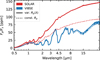 |
Fig. B.1 Comparison between emission flux computed with constant Rp = 1.74 by HELIOS (dotted) and including the wavelength-dependent extension in radius Rp(λ) by the atmosphere, obtained with Eq. B.2. The synthetic spectra are for a SOLAR and a VIBSE case, respectively, both with Tirr =2500 K, Mp = 8M⊕, ΔIW0 and ΨVMF =0. |
Appendix C Average mean molecular weight
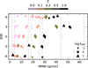 |
Fig. C.1 Average MMW of atmospheres from our grid at Tirr = 2500 K. The MMW does not vary significantly with altitude. Note that the individual cases in ΨVMF have been plotted with small offsets on the y-axis (ΔIW) to enhance visual clarity. |
Appendix D Opacities
Opacity species, sources and validity ranges.
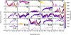 |
Fig. D.1 Unweighted opacities used in this study. Species are shown over a range of temperatures, if available. The pressure is 0.01 bar for molecules and CIAs, but for the atomic species, only 10−8 bar are available. |
Appendix E Collision-induced absorption
Here, we assess the effect of CIA relative to the opacities of dominant molecular species. The available CIA pairs relevant for the high-temperature conditions in HRE atmospheres are H2–H2, H2–H, and H2–He. The collision line-lists of other dominant gases, e.g. CO2-CO2, have no experimental or theoretical support in the temperature range of interest. CIA scales primarily with pressure, in contrast to the opacities of triatomic molecules such as H2O, CO2, and SO2 that show stronger response to temperature.
As shown in Sect. 3.2, the photospheres are located at low pressure (typically in the ~10−1–10−6 bar range) for any combination of ξ, ΨVMF, and fO2. These altitudes are well above the pressure levels at which CIA opacities become comparable to molecular opacities (~1 − 100 bar). At such high pressures, HRE atmospheres can reach temperatures of ~3000 K, for which even the high-temperature CIA line lists are currently unavailable. As a result, our model cannot self-consistently include CIA effects under these conditions. However, given the relatively grey nature of CIA opacity in the infrared, we expect their primary effect to be a general greying of the spectrum in the wavelength range where most energy transport occurs (i.e. at infrared wavelengths corresponding to T ~ 3000 K). Consequently, CIAs are unlikely to significantly affect the radiative transfer in atmospheres that are already optically thick due to strong absorbers like CO2, SO2, and especially H2O.
To test this hypothesis, we performed simulations for a ΨVMF = 0, ΔIW-6 atmosphere at both ξ =0 (SOLAR) and ξ =1 (VIBSE), including CIA contributions from H2–H2 and H2–He. The results (Fig. E.1) confirm that the effect of CIA is negligible at both Tirr = 2500 K and 1500 K. This specific choice of ΨVMF =0 and ΔIW-6 corresponds to the part of the parameter space were we expect CIAs to be most pronounced, i.e. H2-rich atmospheres.
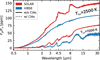 |
Fig. E.1 Negligible effect of CIAs on emission spectra. |
Appendix F Intrinsic temperature
Earlier results on HRE atmospheres showed that elevated Tint can lead to heating of lower layers and onset of convection (Zilinskas et al. 2023; Nicholls et al. 2025a). We tested these findings by varying Tint from 0 to 300 K for SOLAR and VIBSE atmospheres at ΔIW-3 and ΔIW+3, but recover little impact for SOLAR-like atmospheres for Tint < 200 K and no impact on VIBSE-like atmospheres at any Tint (Fig. F.1). The oxidised SOLAR-case seems to be marginally more sensitive to the choice of Tint.
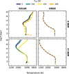 |
Fig. F.1 Effect of intrinsic temperature, Tint, on P-T-profiles. |
A leave-one-out-test on the opacities (not shown) confirms that mainly H2O is responsible for the increase in temperature of the bottom layers seen in SOLAR-cases at Tint ≳ 200 K in Fig. F.1. As underlying reason we identify its strong and effectively grey opacity compared to other major gases like H2, He, CO2, CO and SO2 (Fig. D.1). In highly opaque atmospheres, the contribution of the intrinsic temperature is enhanced and becomes dominant above a certain value of Tint, based on the opacity structure (cf. Guillot 2010, their Eq. 29); comparison of these contributions indicate that in SOLAR-like atmospheres, Tint starts to dominate at ~200-300 K, while VIBSE-like atmospheres should remain unaffected (i.e. dominated by Tirr), consistent with our findings. Since H2O is more abundant in SOLAR-like atmospheres (see Fig. 4), and there particularly in oxidised cases, these atmospheres tend to be most sensitive to Tint. Once the intrinsic temperature modifies the P-T-profile, the atmosphere quickly enters a positive feedback loop where rising temperatures force greater fO2 for a given ΔIW, in turn producing more H2O. Hence, no converging solution for Tint = 300 K could be found for the oxidising SOLAR case in Fig. F.1.
Regarding convective stability, we found that the sharp increase in surface temperature pushes the atmosphere towards violation of the Schwarzschild-criterion (albeit not exceeding it), potentially inducing some small-scale convection in the lower layers of the planetary atmosphere, close to the magma ocean. However, this analysis is only valid for the tested case, Tirr =2500 K. Cooler atmospheres host lower radiation fluxes, and thus, a given value of Tint should have a stronger effect, potentially leading to significant modification of the atmospheric P-T-profile, including the onset of convection which we found to be suppressed in the canonical models studied here (cf. Nicholls et al. 2025a).
Appendix G Extended vapour series
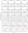 |
Fig. G.1 Partial pressures of exsolved vapours for a wide range of conditions. The temperature at the MAI is 3000 K. Greyed-out axes highlight the onset of non-ideality, with greater deviation from the ideal gas law indicated by more desaturated grey. |
Appendix H Emission spectra at varying temperatures
Appendix I 55 Cnc e, MIRI constraints
Here we report the detailed results from the χ2-analysis presented in Sect. 4.2. We evaluated the χ2 for the MIRI observation (Hu et al. 2024) for all emission spectra from Fig. 7, and show them in Fig. I.1. The upper threshold value of χ2 was chosen such that the percentile point function is 0.95; a model that has a χ2 worse than this is considered non-fitting. Our model has seven degrees of freedom (corresponding to the number of data points in the MIRI observation, excluding the shadow region; see Fig. 11), which yields a threshold value of ~14.
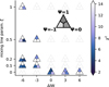 |
Fig. I.1 Models that fit the MIRI LRS observation, ranked by the χ2 metric. Each segment of the triangular glyphs reports the χ2 of all tested ΨVMF (−1, 0, 1) at given ΔIW (x-axis) and ξ (y-axis). Cases were no fitting solution was found are greyed out. |
Appendix J Acetylene Worlds
Acetylene, C2H2, emerges under C-rich but H- and O-depleted conditions (see Fig. J.1), typically found in highly reducing (ΔIW ≲ − 3), high ΨVMF (≳ 0) and VIBSE-like (z ~ 1) scenarios. Compared to methane (CH4), acetylene appears preferentially in hot atmospheres (≳ 2000 K, cf. Fig. G.2 and G.1). As major opacity source in the infra red (Fig. D.1), it may become the dominant absorber, overpowering HCN; in cooler atmospheres (Tirr ≲2000 K), methane begins to replace C2H2 (Fig. H.2).
However, the line lists of both CH4 (Yurchenko & Tennyson 2014) and C2H2 (Chubb et al. 2020) terminate at 0.8/1 μm, respectively, and thus lack opacity in the vital UVIS where a significant fraction of the stars energy is input into the atmosphere. The rapid cut-off induces an artificial and pronounced greenhouse-effect; the BOA temperatures are raised by ~250 K by a scenario where C2H2 is included in the radiative transfer simulation versus a scenario without (Fig. J.2, left column). The abrupt change in opacity at 1 μm becomes evident in the emission spectrum as artificial feature that strongly affects both tested oxidation states equally, ΔIW-3 and ΔIW-6 (Fig. J.2). The effect of both acetylene and methane quickly dies off with increasing oxygen content, as both gases vanish; atmospheres with ΔIW ≳ −2 or ΨVMF <0 are never affected.
Due to the limitation in the line list and the artificial changes to the pressure-temperature structure and the spectra of ultra-HREs, we omitted C2H2 from the opacity, but remark that the affected atmospheres in Fig. 7 and 8 are ΔIW-6 for ΨVMF =0 and ΔIW-6 and ΔIW-3 for ΨVMF =1; in all other atmospheres, the effect of acetylene is not relevant. In the absence of C2H2 as absorber, HCN and CO take precedence (see Fig. 8). However, these spectra are likely inaccurate, and subject to change once newer line lists can be obtained.
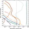 |
Fig. J.1 Chemistry as function of altitude in a ΨVMF =1, ξ =1, ΔIW-3 planet at Tirr =2500 K. |
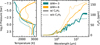 |
Fig. J.2 Effect of acetylene on the atmospheric structure and spectra of reducing and heavy atmospheres (ΔIW ≤ −3, ΨVMF =1, ξ =1). |
All Tables
Target species with solubility laws for the Atmodeller chemical network. Table adopted from Bower et al. (2025).
All Figures
|
Fig. 1 Bulk volatile (mass) ratios of volatiles as a function of ξ. |
| In the text | |
|
Fig. 2 Partial pressures of gas species at the magma ocean–atmosphere interface (MAI) as function of fO2, ΨVMF, and ξ. All atmospheres were simulated at TMAI = 3000 K and Mp = 8 M⊕. |
| In the text | |
|
Fig. 3 Faction of the budget of a given element E ∈ {H, He, C, N, O, S} that resides in the atmosphere (Eatmo/Etotal), where “total” refers to the mass-weighted sum of atmosphere plus mantle. The dotted black line, log10-zero, denotes the level at which the entirety of an element would reside in the atmosphere. |
| In the text | |
|
Fig. 4 Detailed atmospheric structures for a selected set of synthetic hot rocky exoplanets (ΨVMF =0, Mp =8 M⊕, Tirr =2500 K). Column 1: optical depth τ as function of wavelength and atmospheric pressure altitude. The photosphere, defined where the atmosphere has absorbed 50% of all incoming light, is indicated as solid white line; the 25% and 75% levels are shown in dotted white lines. Column 2: pressure–temperature structure. Column 3: speciation as function of pressure altitude. |
| In the text | |
|
Fig. 5 Atmospheric thermal structure for representative scenarios. The pressure-temperature profiles for each simulated model is shown in colour, according to its oxygen fugacity, and the line style shows the Tirr of the model. Vertical grey lines indicate the irradiation temperature of the respective simulation. |
| In the text | |
|
Fig. 6 Condensation degrees of elements (i.e. number fraction of an element that has condensed relative to its total atmospheric abundance) as function of atmospheric altitude for the Tirr =2500 K cases in the grid in Fig. 5. The colour denotes the element (red – Si, blue – Mg, teal – O, black – C, yellow – Fe), and the line style indicates the composition (solid – VIBSE; dashed – SOLAR). The pressure-temperature structure (at arbitrary units) is shown in light grey. The identity of condensates that occur in the respective atmospheres are SiC (silicon carbide), graph (graphite), fo (forsterite; Mg2SiO4), fa (fayalite; Fe2SiO4), qtz (quartz; SiO2), en (enstatite; MgSiO3), per (periclase; MgO), hem (hematite; Fe2O3), and mag (magnetite; Fe3O4). |
| In the text | |
|
Fig. 7 Synthetic emission spectra over a grid in ΔIW ∈ {−6, −3, 0, +3, +6} (colour), ξ ∈ {0, 0.1, 0.2, 0.5, 1} (row) and ΨVMF ∈ {−1, 0, 1} (column). Other parameters were kept constant: Mp = 8M⊕, xmelt = 1 (fully molten mantle), Tirr =2500 K. Important broad-band spectral features are highlighted by coloured patches. The 4.5 μm feature, where multiple bands coalesce, is labelled 4.5r when reducing species (CO + SiO) dominate and 4.5o when oxidising species (CO2 + SO2) dominate. |
| In the text | |
|
Fig. 8 Transmission spectra of the synthetic atmospheres from Fig. 7 rearranged to highlight the effect of ξ, which was (nearly) absent in emission. The spectra are reported in terms of the scaled density, Eq. (13), which at constant mass (here, Mp = 8M⊕) can be directly related to the radius (right axis). Prominent spectral features are highlighted by coloured bands. |
| In the text | |
|
Fig. 9 Mass versus the scaled density for observed (dots) and modelled planets (lines). Scaled density is defined as ρ/ρ⊕, where ρ⊕(M) is the density of a planet with the same interior structure and composition as Earth at a given mass (M). The radii of the modelled planets are based on the radius of the photosphere, which was averaged over the Kepler bandpass. The curves for atmosphere-bearing planets are computed for endmember cases (ξ = VIBSE, SOLAR; ΔIW = −3, +3; Tirr = 1250 K, 2500 K, at constant ΨVMF =0). Curves for two atmosphere-free cases (a coreless planet; CORL and a BSE-like planet, BSE) are also shown. The points denote a collection of measured masses and radii for planets R ≤ 4 R⊕, M ≤ 10 M⊕ and Tirr ≥ 1000 K, obtained from the NASA Exoplanet Archive; we omit objects with an uncertainty σρscaled > 0.25 from the plot. |
| In the text | |
|
Fig. 10 Average scaled density of the synthetic models from Fig. 8 in the Kepler/TESS bandpass (400–900 nm), shown as a function of ΔIW and ΨVMF (coloured lines and dots). The colour corresponds to ξ. The simulations are compared to the inferred scaled densities for 55 Cancri e and TOI-1408 c, which are shown as grey bands; their width denotes the 1σ limit. The dashed black line indicates the scaled density of an atmosphere-free (airless) planet, i.e. Rp,MAI (Sect. 2.1.1). |
| In the text | |
|
Fig. 11 Observations from MIRI of 55 Cancri e (black markers, Hu et al. 2024), including the MIRI shadow region (orange markers), compared to a selection of synthetic emission spectra (coloured and grey lines). The blue shaded area indicates the range of spectra that matches the observation, based on a χ2-fit (excluding the shadow region). Three endmembers within the set of matching models are highlighted: the best fit (black, ΨVMF = 0, ΔIW-6 and ξ = 0.5), a mineral-rich He–H2–CO–SiO–atmosphere (minC, bright blue, ΨVMF = −1, ΔIW-6 and ξ = 0.1), and a waterworld (WW, dark blue, ΨVMF = 1, ΔIW+6 and ξ = 0). Relevant non-fitting models are shown in grey and comprise the gas-dwarf scenario (GDw, ΨVMF = 1, ΔIW-6 and ξ =0) as well as a reduced (rBSE, ΨVMF = 0, ΔIW-3 and ξ =1) and an oxidised VIBSE scenario (oBSE, ΨVMF = 0, ΔIW+3 and ξ = 1). |
| In the text | |
|
Fig. 12 Prediction for MIRI MRS MEDIUM channel observations of 55 Cancri e for selected synthetic atmospheric models (identical to Fig. 11). Uncertainties were simulated via the pandeia.engine package (v4.0) (Exposure Time Calculator, ETC, Pontoppidan et al. 2016) with JWST reference data (Space Telescope Science Institute 2024), assuming 7 groups and 19.4 seconds per exposure. Only channels 1, 2 and 3 are shown (CH1-CH3); channel 4 at 25 μm is unlikely to yield useful constraints owing to its low through-put. |
| In the text | |
|
Fig. B.1 Comparison between emission flux computed with constant Rp = 1.74 by HELIOS (dotted) and including the wavelength-dependent extension in radius Rp(λ) by the atmosphere, obtained with Eq. B.2. The synthetic spectra are for a SOLAR and a VIBSE case, respectively, both with Tirr =2500 K, Mp = 8M⊕, ΔIW0 and ΨVMF =0. |
| In the text | |
|
Fig. C.1 Average MMW of atmospheres from our grid at Tirr = 2500 K. The MMW does not vary significantly with altitude. Note that the individual cases in ΨVMF have been plotted with small offsets on the y-axis (ΔIW) to enhance visual clarity. |
| In the text | |
|
Fig. D.1 Unweighted opacities used in this study. Species are shown over a range of temperatures, if available. The pressure is 0.01 bar for molecules and CIAs, but for the atomic species, only 10−8 bar are available. |
| In the text | |
|
Fig. E.1 Negligible effect of CIAs on emission spectra. |
| In the text | |
|
Fig. F.1 Effect of intrinsic temperature, Tint, on P-T-profiles. |
| In the text | |
|
Fig. G.1 Partial pressures of exsolved vapours for a wide range of conditions. The temperature at the MAI is 3000 K. Greyed-out axes highlight the onset of non-ideality, with greater deviation from the ideal gas law indicated by more desaturated grey. |
| In the text | |
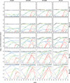 |
Fig. G.2 Similar to Fig. G.1, but with T=2000 K. |
| In the text | |
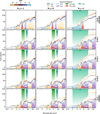 |
Fig. H.1 Similar to Fig. 7, but for Tirr =2000 K. |
| In the text | |
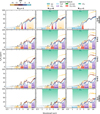 |
Fig. H.2 Similar to Fig. 7, but for Tirr =1500 K. |
| In the text | |
|
Fig. I.1 Models that fit the MIRI LRS observation, ranked by the χ2 metric. Each segment of the triangular glyphs reports the χ2 of all tested ΨVMF (−1, 0, 1) at given ΔIW (x-axis) and ξ (y-axis). Cases were no fitting solution was found are greyed out. |
| In the text | |
|
Fig. J.1 Chemistry as function of altitude in a ΨVMF =1, ξ =1, ΔIW-3 planet at Tirr =2500 K. |
| In the text | |
|
Fig. J.2 Effect of acetylene on the atmospheric structure and spectra of reducing and heavy atmospheres (ΔIW ≤ −3, ΨVMF =1, ξ =1). |
| In the text | |
Current usage metrics show cumulative count of Article Views (full-text article views including HTML views, PDF and ePub downloads, according to the available data) and Abstracts Views on Vision4Press platform.
Data correspond to usage on the plateform after 2015. The current usage metrics is available 48-96 hours after online publication and is updated daily on week days.
Initial download of the metrics may take a while.