| Issue |
A&A
Volume 709, May 2026
|
|
|---|---|---|
| Article Number | A186 | |
| Number of page(s) | 9 | |
| Section | Galactic structure, stellar clusters and populations | |
| DOI | https://doi.org/10.1051/0004-6361/202659689 | |
| Published online | 20 May 2026 | |
Revealing the stellar population of the ultra-obscured Galactic globular cluster Glimpse-C02★
1
Dipartimento di Fisica e Astronomia, Università degli Studi di Bologna,
Via Piero Gobetti 93/2,
40129
Bologna,
Italy
2
INAF – Astrophysics and Space Science Observatory Bologna,
Via Piero Gobetti 93/3,
40129
Bologna,
Italy
3
Institute for Astronomy, University of Edinburgh, Royal Observatory,
Blackford Hill,
Edinburgh
EH9 3HJ,
UK
4
Department of Astronomy, Indiana University,
Bloomington,
Swain West, 727 E. 3rd Street,
IN
47405,
USA
★★ Corresponding author: This email address is being protected from spambots. You need JavaScript enabled to view it.
Received:
3
March
2026
Accepted:
29
March
2026
Abstract
In this paper, we present the results of a detailed photometric analysis of Glimpse-C02, one of the most extincted globular clusters of the Milky Way. We built a deep color magnitude diagram spanning ≈10 magnitudes and enabling the very first identification of the main sequence turnoff of the cluster. Due to the extreme reddening conditions of the region where the stellar system is located, a differential reddening correction was necessary. The resulting reddening map shows color excess variations up to δE(B − V) ≈ 2.5 mag in the direction of the target. From isochrone-fitting of the differential reddening corrected color-magnitude diagram, we obtained a new estimate of the mean color excess, E(B−V) = 6.33−0.04+0.05, and a distance modulus (m−M)0 = 14.00−0.11+0.26, corresponding to a distance of d = 6.3−0.3+0.8 kpc from the Sun, and a Galactocentric distance of 2.6−0.7+0.6 kpc. This distance value, within the associated uncertainties, suggests that the cluster may be located closer to the Galactic Center compared to previous estimates, possibly supporting its classification as a bulge globular cluster. Furthermore, we obtained a photometric metallicity estimate of [Fe/H] = −0.30−0.08+0.10 and the first absolute age determination for Glimpse-C02, resulting in t = 11.9−0.6+0.7 Gyr, as typically measured for Galactic globular clusters at this metallicity. We also obtained a new estimate of the center of gravity of the cluster and determined its projected density profile from resolved star counts, finding a high King concentration parameter (c = 1.97−0.67+0.51) and a core radius rc = 8.72−0.35+0.40 arcsec. Finally, from the surface brightness profile of the system, we derived an integrated H-band magnitude MH = −7.9, corresponding to a mass of M = 3.57−0.19+0.22 × 10⁴ M⊙. Thus, our work classifies Glimpse-C02 as an old and metal-rich globular cluster that is in an advanced stage of its dynamical evolution.
Key words: Hertzsprung–Russell and C–M diagrams / stars: Population II / Galaxy: stellar content / globular clusters: individual: Glimpse-C02
Based on observations with the NASA/ESA HST, obtained under program GO 17918 (PI: Loriga). The Space Telescope Science Institute is operated by AURA, Inc., under NASA contract NAS5-26555.
© The Authors 2026
 Open Access article, published by EDP Sciences, under the terms of the Creative Commons Attribution License (https://creativecommons.org/licenses/by/4.0), which permits unrestricted use, distribution, and reproduction in any medium, provided the original work is properly cited.
This article is published in open access under the Subscribe to Open model. This email address is being protected from spambots. You need JavaScript enabled to view it. to support open access publication.
1 Introduction
The Milky Way (MW) hosts ∼170 globular clusters (GCs), a large fraction of which have been extensively studied, both photometrically and spectroscopically, using both space- and ground-based facilities (see, e.g., Carretta et al. 2009; Valenti et al. 2010; Kamann et al. 2018; Libralato et al. 2022; Ferraro et al. 2018a,b, 2023, 2026a). As the oldest stellar systems in our Galaxy (see, e.g, Marín-Franch et al. 2009; Dotter et al. 2010; VandenBerg et al. 2013; Valcin et al. 2020; Massari et al. 2023; Aguado-Agelet et al. 2025; Ceccarelli et al. 2025), they are key tracers of the early evolution of the MW, providing important insights into its formation and assembly history (Massari et al. 2019). In this context, it is worth mentioning that two stellar systems, formerly classified as bulge GCs, Terzan 5 and Liller 1, have been found to exhibit properties that are incompatible with those of genuine GCs, such as the presence of multi-iron and multi-age subpopulations (Ferraro et al. 2009, 2016, 2021). Their properties suggest that they could be fossil remnants of more massive structures that contributed to the formation of the bulge (see also Lanzoni et al. 2010; Origlia et al. 2011, 2013, 2019, 2025; Massari et al. 2014; Pallanca et al. 2021a; Dalessandro et al. 2022; Crociati et al. 2023, 2024; Alvarez Garay et al. 2024; Fanelli et al. 2024; Ferraro et al. 2025) and could represent a significant source of gravitational waves (Ferraro et al. 2026b). This reinforces the urgency to extend the investigation of Galactic GCs to include stellar systems that have been poorly studied so far because they are located in observationally challenging regions. In fact, a proper characterization of star clusters in regions such as the bulge and the disk has often been hampered by extreme obscuration due to interposed dust along the line of sight, and by severe stellar crowding.
Near-infrared (NIR) surveys such as the Two Micron All Sky Survey (2MASS; Skrutskie et al. 2006), the VISTA Variables in the Via Lactea (VVV) survey (Minniti et al. 2010) and its extension VVVX (Minniti 2016), together with mid-infrared surveys, such as the Galactic Legacy Infrared Mid-Plane Survey Extraordinaire (GLIMPSE; Benjamin et al. 2003) and the Wide-field Infrared Survey Explorer (WISE; Wright et al. 2010), have been fundamental for the study and the discovery of previously unknown GCs in the MW bulge and disk. Various methods have been employed to identify and confirm potential star clusters, for example, by building density maps to visually detect the presence of overdensities (Minniti et al. 2017). However, since not all overdensities correspond to real clusters, one of the most reliable approaches is represented by a kinematic analysis, especially exploiting the high precision of Gaia proper motions (see, e.g., Garro et al. 2020, 2021; Obasi et al. 2021; Minniti et al. 2021a), to distinguish between cluster members and galactic field interlopers and to determine the real nature of the stellar system. Still, Gaia works mainly in the optical band, and the limiting magnitude in the G band is ∼20, which is not enough to perform a complete kinematic analysis of the systems. Moreover, only a fraction of the discovered stellar systems have been analyzed so far (Froebrich et al. 2007; Borissova et al. 2014; Minniti et al. 2017, 2021a, 2021b; Camargo 2018; Palma et al. 2019; Camargo & Minniti 2019; Garro et al. 2020, 2021; Obasi et al. 2021; Dias et al. 2022; Garro et al. 2022; Kader et al. 2022, 2023; Kunder et al. 2024; Hughes et al. 2026, among others) and current ground-based infrared (IR) facilities are not sufficient to completely characterize these objects. So, a very precise, high-resolution IR study is needed, exploiting, for example, the superb capabilities of the Hubble Space Telescope (HST).
In this context, we present the first accurate photometric analysis of Glimpse-C02, one of the most extincted GCs of the MW. It was discovered in the GLIMPSE project (Benjamin et al. 2003), which offered an excellent opportunity to explore a very extincted region of our galaxy, thanks to the use of NIR wavelengths, and to provide a deep census of reddened MW GCs. Glimpse-C02 is situated near the Galactic plane (l = 14◦.129, b = −0◦.644; see N.3 in Mercer et al. 2005), inside the thin disk, between its inner edge and the transition region with the bulge, at a distance D ≈ 4.6 ± 0.7 kpc, based on the brightnesses of the red clump (RC) and the tip of the red giant branch (RGB) (Kurtev et al. 2008). It is a heavily extincted stellar system (AV ≈ 24.8 ± 3) that, according to moderate resolution K-band spectra of three probable members, has a metallicity [Fe/H]= −0.33 ± 0.14 (Kurtev et al. 2008). However, these results were obtained with the ground-based instrument SofI at the New Technology Telescope (NTT), which allowed the identification of just a portion of the RGB of the cluster, considering a region of 60″ from the center (see Figure 2 of Kurtev et al. 2008). Hence, the high-resolution and NIR capabilities of the HST WFC3/IR camera represent an unprecedented opportunity to fully characterize this stellar system photometrically.
This work is organized as follows. Section 2 describes the NIR datasets used in the analysis and the adopted data analysis procedures. In Section 2.3, we present the derived color–magnitude diagrams (CMDs) and discuss the main characteristics of the evolutionary sequences. Section 3 describes the method adopted to build the differential reddening map in the direction of the cluster. In Section 4, we show a comparison with a well-known bulge GC (NGC 6440) that is characterized by a similar value of metallicity, while Section 5 is focused on the estimate of the absolute age of Glimpse-C02 through isochrone fitting and the determination of its distance modulus and color excess. In Section 6, we present a new determination of the center of gravity and of the projected density and surface brightness profiles, which are used to derive the main structural parameters of the system via King model fitting, and to estimate the total luminosity and the mass of the cluster. Finally, in Section 7 we present a summary of the work and the main conclusions.
 |
Fig. 1 WFC3/IR image centered on Glimpse-C02 obtained in the F160W filter, with an exposure time of 199 s. North is up, east is to the left. |
2 Observations and data analysis
2.1 NIR dataset
The photometric investigation of Glimpse-C02 presented in this study is based on the analysis of the first HST epoch of this stellar system (proposal GO 17918, PI: Loriga). It is composed of high-resolution images obtained from the IR channel of the WFC3/HST. This instrument provides a spatial resolution of ∼0.13 arcsec/pixel in a nominal 136 × 123 arcsec2 field of view (FoV). The data were acquired on March 30, 2025 and they are composed of four images obtained in F110W (2 × 399 s, 2 × 299 s) and four images in F160W with an exposure time of 199 s. For the sake of illustration, a F160W image of the studied cluster is shown in Fig. 1.
To determine the stellar density profile along the entire radial extension of the system, we complemented the high-resolution HST data with a set of wide-field near-IR images obtained as part of the VVVX survey (Minniti 2016), as described also in Cadelano et al. (2022). This dataset was acquired with the VISTA InfraRed CAMera (VIRCAM) mounted on the VISTA-ESO telescope. It is composed of two images obtained with the J filter and an exposure time of 120 s, and five images with the Ks filter and an exposure time of 16 s.
2.2 Data reduction
In our photometric analysis, we used flt images, which are already processed and calibrated (i.e., flat-fielded, dark-subtracted) by the Space Telescope Science Institute (STScI) pipeline, as well as drz images, which are calibrated and corrected for geometric distortions. The analysis of the dataset has been performed using DOLPHOT (Dolphin 2000, 2016), a stellar photometry package that was originally created to obtain accurate stellar photometry PSF-fitting with the Wide Field and Planetary Camera 2 (WFPC2) data, but it was then generalized to use analytic PSF models for any camera. The procedure is very similar to the classic point spread function (PSF)-fitting routine, and it also includes an initial image preparation, meaning a masking of bad columns, cosmic-ray cleaning, hot pixel masking, etc.; a sky or background determination and a final aperture corrections evaluation and application to provide a calibrated photometry. DOLPHOT also performs pixel area map (PAM) and charge transfer efficiency (CTE) corrections. In our procedure, we used the drz F160W image as the reference frame for all the other F160W and F110W images, for which the geometric transformations were determined. We set a threshold of 5σ for the inclusion of stars in the final catalog. All remaining parameters were set to the default values for the camera. The final product is a catalog in which the magnitudes from different images are combined using a weighted mean that accounts for the χ2 of the PSF-fitting procedure. Moreover, the magnitudes are reported to the VEGAMAG photometric system, using the appropriate zero points and encircled energy fractions, and including aperture corrections. Furthermore, the final catalog contains several photometric quality flags (e.g., chi, sharpness, roundness) that are useful for preliminary cleaning to remove poorly measured stars. The final necessary step in building the final catalog was to transform the instrumental coordinates to the absolute reference frame (α and δ). To do that, we used the stars in common with the publicly available 2MASS catalog (Skrutskie et al. 2006), which was used as a sort of “bridge catalog” to obtain the astrometric information from the Gaia DR3 catalog (Gaia Collaboration 2023), through the cross-correlation software CataXcorr (Montegriffo et al. 1995). In the case of the VIRCAM data, the data reduction was performed using a standard approach suitable for ground-based observations with the DAOPHOT and ALLFRAME packages (see, e.g., Loriga et al. 2025). The resulting catalog was astrometrized using the stars in common with the Gaia DR3 catalog (Gaia Collaboration 2023) and the instrumental magnitudes were calibrated using the stars in common with the 2MASS catalog (Skrutskie et al. 2006), obtained with the same filters and in an overlapping region of the sky. The derived CMD is shown in the right panel of Fig. 2.
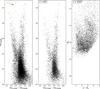 |
Fig. 2 Left panel: (mF160W, mF110W − mF160W) observed CMD of Glimpse-C02 after the cleaning procedure using roundness, sharpness and chi parameters, with the reddening vector shown as a red arrow. Central panel: (mF160W, mF110W − mF160W) observed CMD of Glimpse-C02 after the same cleaning procedure and by considering a radius of 45″ from the center, as determined in Sect. 6. Right panel: (Ks, J − Ks) CMD for distances beyond 250″ from the center, obtained from the analyzed VIRCAM data. |
2.3 NIR CMD of Glimpse-C02
The CMD obtained from the analyzed observations is shown in the left panel of Fig. 2, after applying a cleaning procedure based on the chi, sharpness, and roundness parameters, using a 3σ clipping criterion. The central panel of the same figure shows the CMD that includes only stars located within a radius of 45″ from the system’s center of gravity, as defined in Sect. 6. This represents the first CMD of Glimpse-C02 ever obtained from high-resolution HST data, and its comparison with previous results published in the literature (see Fig. 2 of Kurtev et al. 2008) allows us to fully appreciate the advantages of using space-based high-resolution IR data. By analyzing the CMD, it is possible to identify, for the first time for this stellar system, the main sequence turnoff (MS-TO), which is located around mF160W ≈ 20 (mF110W ≈ 23). The CMD extends ≈3 mag below it. However, the effect of differential reddening is evident as a huge spread of all the evolutionary sequences, which are also affected by intense field contamination, as clearly visible mainly in the left part of the CMD. Unfortunately, it is not possible to decontaminate the cluster population from field interlopers. In fact, no second epoch observations exist to measure relative proper motions and discriminate cluster members from Galactic field interlopers. We also searched for stars in common with Gaia DR3 (Gaia Collaboration 2023), but only a few matches with measured proper motions were found, mostly located in CMD regions typical of field stars, thus preventing a reliable decontamination. In addition, no complementary observations of the field surrounding the cluster are available to perform a statistical decontamination (e.g., Dalessandro et al. 2008, 2019; Giusti et al. 2023; Rosignoli et al. 2026).
Despite all this, the presence of a well-populated and extended RGB, which is a characteristic commonly associated with old stellar systems, can be clearly recognized in the CMD. Moreover, the lack of a blue horizontal branch (HB) suggests a likely metal-rich GC, which is in agreement with the spectroscopic analysis of Kurtev et al. (2008). A low-significance over-density along the RGB at magnitudes mF110W ≈ 19.5 and mF160W ≈ 16.5 suggests the presence of the red clump typical of metal rich-populations.
3 Differential reddening
One of the main challenges in characterizing Glimpse-C02 is represented not only by the presence of strong interstellar extinction but also by its spatial variability along the line of sight. This is known as differential reddening and is due to the presence of clouds with different column densities on scales as small as a few arcsec (see, e.g., Pallanca et al. 2021a). As a consequence, the amount of color excess E(B − V), defined as the difference between the observed color (B − V) and the intrinsic one (B − V)0, varies from star to star depending on their position within the observed field. The primary effect on the CMD is a stretching of the evolutionary sequences along the reddening vector. To correct the CMDs for this effect, the first step consists of the assumption of the “reddening law” (see, e.g., Cardelli et al. 1989; Fitzpatrick & Massa 1990; O’Donnell 1994; Fitzpatrick 1999), which means the wavelength dependence of interstellar extinction relative to the absolute extinction in the V-band. Indeed, the direction of the reddening vector in a CMD depends on the photometric filters adopted, through wavelength-dependent parameters commonly referred to as Rλ. These parameters are related to the extinction coefficients via the relation Aλ = Rλ × E(B − V). Each Rλ can be expressed as the product of two terms:  . Here,
  corresponds to the ratio Aλ/AV (or equivalently, Rλ/RV), which describes the reddening law. In our case, we assume the standard reddening law described by Cardelli et al. (1989) with RV = 3.1, corresponding to RF110W = 1.04345 and RF160W = 0.63296.
To perform the differential reddening correction, we adopted a star-by-star approach, described in detail by Pallanca et al. (2019, see also Cadelano et al. 2020; Pallanca et al. 2021a; Loriga et al. 2025). The method consists in determining the mean ridge line (MRL) of Glimpse-C02 in the NIR CMD by selecting a sample of well-measured, likely member stars located along the RGB, sub-giant branch, and upper MS. For each star in our HST catalog, we then identified a group of nearby N∗ = 30 stars (selected within a maximum radius of 10″) that were also well measured. This group, composed of N∗ stars, was used to construct a so-called “local CMD”. To estimate the differential reddening that affects each star, we shifted the MRL along the reddening vector in steps of δE(B − V) until it matched the local CMD. The differential reddening map obtained from this procedure is shown in Fig. 3 on a FoV of roughly 136 × 123 arcsec2, corresponding to the nominal FoV of the WFC3. In the figure, only regions with reliable differential reddening corrections are shown. As can be seen, the reddening appears patchy, with different regions characterized by different reddening features. On the western side of the FoV it is possible to distinguish a highly reddened region (darker colors). The same holds for the southern side, where a more elongated filament is observed, and in the northwest part of the map. A small dark blob can also be noticed in the north with respect to the center of the cluster (black cross; see Section 6). Some lighter blobs, meaning smaller values of differential reddening, can be seen in the northwest region of the FoV, as well as in the eastern part. Overall, the map graphically indicates an extremely large variation in the extinction, reaching a maximum value of δE(B − V) ≈ 2.5 mag in the whole FoV.
The derived reddening map has been applied to correct the effects of differential reddening in the observed CMDs (see Fig. 4). A residual differential reddening is likely still present in the CMD, as shown in the right panel of Fig. 4, where the red crosses indicate the 3σ mean magnitude and color uncertainties in each magnitude bin, which are smaller than the residual width of the sequences. However, overall, the significant improvement achieved through the correction is clearly visible, particularly in the RGB of the central panel of Fig. 4, as well as in the MS-TO region, which appears noticeably sharper and better defined.
 |
Fig. 3 Differential reddening map relative to the cluster center position (black cross; see Sect. 6). North is up, east is to the left. Darker colors correspond to more extincted regions, as detailed in the side color bar that reports the differential color excess δ(B − V). |
4 Comparison with NGC 6440
First, given the complexity of Glimpse-C02, we adopt a qualitative approach that consists of comparing the CMD of this system with that of the well-studied bulge GC NGC 6440. The comparison can provide first-guess values of the distance and mean color excess of Glimpse-C02. Indeed, NGC 6440 provides a useful reference, as its metallicity ([Fe/H] = −0.56, Origlia et al. 1997, 2008) is similar to that of Glimpse-C02. Moreover, NGC 6440 was observed with the same HST WFC3/IR filters as Glimpse-C02, thus allowing for a straightforward comparison between the two. In particular, the dataset (Proposal GO 12517, PI: F.R. Ferraro) is composed of eight images obtained in the F160W filter (1 × 26 s and 7 × 249 s) and eight images in F110W (1 × 26 s and ×7 × 349 s). For this cluster, we performed the same reduction procedure for Glimpse-C02 described in Sect. 2.2, using an F160W drz image as a reference. The distance modulus of NGC 6440 ((m − M)0 = 14.6), together with its age (t = 13 Gyr) and reddening (E(B − V) = 1.27), has been accurately determined by Pallanca et al. (2021b, see also Cadelano et al. 2017b, 2023). Therefore, by using the differential reddening-corrected CMD of Glimpse-C02 in the absolute plane, using the values of distance modulus and color excess from Kurtev et al. (2008), we evaluated the MRL of the system, considering only stars located around the HB, RGB and the upper part of the MS, meaning most likely belonging to the cluster. We then constructed the MRL of NGC 6440 and shifted the one of Glimpse-C02 until they matched (right panel of Fig. 5). The values that minimize the color and magnitude difference between the two MRLs have been used to obtain first-guess estimates of the distance modulus and mean color excess for Glimpse-C02: (m − M)0 = 14.0, E(B − V) = 6.4 (left panel of Fig. 5). The very good match between the two CMDs and MRLs suggests that Glimpse-C02 has an age and a metallicity comparable to those of NGC 6440.
 |
Fig. 4 (mF160W, mF110W − mF160W) CMD before the correction for differential reddening (left panel), after the correction for differential reddening (central panel), and after the correction for differential reddening by considering only the stars within 45″ from the center, as defined in Sect. 6 (right panel). The reddening vector is represented in the left panel as a red arrow. The red crosses in the right panel represent the 3σ mean uncertainties on the color and the magnitude for each magnitude bin. |
5 Age and distance determination
Starting from the first-guess values of the distance modulus and reddening of Glimpse-C02 obtained from the superposition of its CMD onto that of NGC 6440, we refined both estimates and determined the age and metallicity of the cluster via the isochrone fitting technique. In this approach, the observed CMD of the cluster is compared with a set of theoretical isochrones to simultaneously estimate age, reddening, distance modulus, and metallicity. To explore the parameter space and derive the best-fit solution, we used the Markov Chain Monte Carlo (MCMC) approach described in Cadelano et al. (2020, see also Deras et al. 2023, 2024; Giusti et al. 2024; Giusti et al. 2025), implemented through the emcee code (Foreman-Mackey et al. 2013, 2019). We adopted the Bag of Stellar Tracks and Isochrones (BaSTI) isochrones (Hidalgo et al. 2018; Pietrinferni et al. 2021, 2024), with [α/Fe]= 0.4, a standard He abundance of Y = 0.247, and including overshooting as well as RGB mass loss. We assumed flat priors for the age, spanning from 2 to 14 Gyr in steps of 0.1 Gyr, and metallicities in the range −1 < [Fe/H] < 0.2 with steps of 0.05 dex. Moreover, Gaussian priors centered on the values obtained from the comparison with NGC 6440, with a σ = 0.1, were adopted for E(B − V) and (m − M)0. The left panel of Fig. 6 shows the isochrone that best reproduces the evolutionary sequences for r < 25″ from the center of the system. The complete set of parameters derived by the procedure are:  ,
,  ,
,  , and
, and ![Mathematical equation: $[{\rm{Fe/H}}] = - 0.30_{ - 0.08}^{ + 0.10}$](/articles/aa/full_html/2026/05/aa59689-26/aa59689-26-eq15.png) . The results robustly confirm that Glimpse-C02 is an old system, fully consistent with the indication already suggested by visual inspection of its CMD. Our estimate of the distance
. The results robustly confirm that Glimpse-C02 is an old system, fully consistent with the indication already suggested by visual inspection of its CMD. Our estimate of the distance  appears to be slightly larger than the value of d = 4.6 ± 0.7 kpc published in Kurtev et al. (2008). The corresponding distance from the Galactic center is
  kpc, smaller than the literature one. The mean color excess is significantly smaller than the literature value, namely, E(B − V) = 7.85 (Harris 1996; Kurtev et al. 2008). A good agreement within the uncertainties is found, instead, for the derived value of [Fe/H].
 |
Fig. 5 Left panel: superposition of the (MF160W, MF110W − MF160W) CMD of Glimpse-C02 (red dots) with the (MF160W, MF110W − MF160W) CMD of NGC 6440 (black dots) in the absolute plane. The parameters used for each GC are labeled. Right panel: (MF160W, MF110W − MF160W) CMD of Glimpse-C02 in the absolute plane with the MRL of NGC 6440 (blue line) and Glimpse C02 (red line) superposed. |
 |
Fig. 6 Left: differential reddening corrected (mF110W, mF110W − mF160W), (mF160W, mF110W − mF160W) CMDs of stars within 25″ from the cluster center and with over-plotted the BaSTI isochrone (red line) that best reproduces the evolutionary sequences of Glimpse-C02. The shaded orange region represents the 1σ uncertainty region of the best-fit isochrone. Right: corner plot with the one- and two-dimensional projections of the posterior probability distributions for all the parameters as obtained from the BaSTI isochrones. The contours correspond to the 1σ, 2σ, and 3σ levels. The values of the color excess, distance modulus, age and metallicity providing the best match with the data are also labeled. |
6 Determination of the structural parameters
6.1 Radial density profile
The first step in determining the cluster’s density profile is to estimate the system’s center of gravity (Cgrav). In this study, we derived it using resolved star counts, made possible by the high spatial resolution of the data. To determine Cgrav, we computed the barycenter of stars selected within specific magnitude ranges and radial distances, starting from an initial guess value (Harris 1996). This procedure was repeated iteratively, using the barycenter obtained from the previous iteration as the new center. Convergence was achieved when the difference between two successive estimates was less than 0.01″ (see, e.g., Montegriffo et al. 1995; Miocchi et al. 2013; Giusti et al. 2024). The analysis was carried out considering stars selected within four different radial ranges (30″, 35″, 40″, 45″) and three magnitude ranges (20.75 < mF160W < 16.0, 20.5 < mF160W < 16, 19.5 < mF160W < 16.0), restricting the sample to the color range 2.8 < (mF110W − mF160W) < 3.5, in order to mitigate field contamination. Radial distances were chosen to sample the gradient in the surface brightness of the cluster, which becomes noticeable at approximately ≈10″ based on visual inspection of the maps. The faint magnitude limits were selected to guarantee high statistics while avoiding spurious fluctuations due to photometric incompleteness. The bright magnitude cut at mF160W = 16 was applied to exclude saturated stars. The final position of Cgrav was obtained by averaging the 12 barycenter estimates, while its uncertainty was estimated as the standard deviation of the mean. The coordinates of Cgrav thus determined are: αICRS = 18h18m30.54s, δICRS = −16◦58′34.94″, with uncertainties of 0.09″ in the right ascension and 0.25″ in declination. This new estimate differs by 3.12″ from the value quoted by Harris (1996).
After the determination of Cgrav, we proceeded to derive the radial density profile based on resolved star counts (see, e.g., Miocchi et al. 2013; Cadelano et al. 2017a; Beccari et al. 2023; Loriga et al. 2025). To sample the inner ≈60″ from the center, we used the WFC3 dataset. For the cluster’s outer regions (60″ ≤ r ≤ 210″), we used the wide-field VIRCAM dataset. In both cases, the FoV was divided into concentric rings of different sizes, chosen to ensure good statistics. Within each ring, we calculated the stellar density as the number of stars divided by the area. To minimize incompleteness effects in the inner regions, we considered only stars with mF160W < 20, with a cut that was made along the direction of the reddening vector. For the VIRCAM wide-field data, we considered only stars with a magnitude Ks ≤ 14. The VIRCAM profile was then renormalized, by anchoring it to the two outermost radial bins of the WFC3 profile, which are in common between the two profiles. The projected density profile obtained from this analysis is shown in Fig. 7 as empty circles. In the outermost regions, at only 60″ from the cluster center, the profile exhibits a flattening, with the logarithm of the density remaining roughly constant at ∼ −0.7 stars arcsec−2. This is the signature of intense contamination by Galactic field stars. This value was then subtracted from the observed profile and the decontaminated radial density distribution of the cluster is shown as filled circles in Fig. 7. To derive the structural parameters of Glimpse-C02, we adopted the fitting procedure described in Raso et al. (2020); Cadelano et al. (2022). Specifically, we performed an MCMC fitting of the observed density profile using King (1966) models, with flat priors on the fitting parameters, namely the central density, the concentration parameter (c), and rc. Moreover, a χ2 likelihood function was used to derive the best fitting parameters. The resulting best-fit model is shown in Fig. 7 and is characterized by a concentration parameter  , corresponding to a dimensionless central potential
  , and a core radius
  arcsec, a half-mass radius
  arcsec, and a tidal radius
  arcsec.
 |
Fig. 7 Projected density profile of Glimpse-C02 derived from star counts in concentric annuli around Cgrav (empty circles) by combining WFC3 and VIRCAM data. The horizontal dashed segment indicates the Galactic field density, which has been subtracted from the observed points (empty circles) to obtain the background-subtracted profile, shown as filled circles. The solid red line represents the best-fit King model to the cluster’s density profile, with the red stripe indicating the ±1σ range of solutions. The vertical lines denote the positions of the core radius (short dashed line), half-mass radius (dot-dashed line). The values of the main structural parameters obtained from the fitting process are labeled (see details in the text). |
6.2 Surface brightness profile
To double-check the values of the structural parameters and estimate the total luminosity and mass of the cluster, we also analyzed its surface brightness profile. The procedure closely follows that adopted for the stellar density profile (see Sect. 6.1). The WFC3 FoV of a drz F160W-band image was divided into a set of concentric annuli, and each annulus was further subdivided into four angular sectors. The integrated surface brightness of each ring was computed as the average of the four sector values, while the associated uncertainty was estimated as their standard deviation. The resulting surface brightness profile is shown in Fig. 8 (empty circles). The mean surface brightness of the background was estimated from the average of the outermost two data points, yielding a value of µF160W ≈ 18.8 mag arcsec−2. This background level was subtracted from all measurements, producing the decontaminated surface brightness profile (filled circles). The corrected profile was fitted following the same methodology described above, through comparison with a grid of King models. The best-fitting parameters are a dimensionless central potential  , a King concentration index
  , a central surface brightness
  mag arcsec−2, a core radius
  arcsec , a half-mass radius
  arcsec, and a tidal radius
  arcsec. All these parameters are consistent, within the uncertainties, with those derived from the fit to the stellar density profile. It is worth emphasizing that the parameters W0 and c match exactly.
To estimate the integrated absolute magnitude of the system, we assumed the distance modulus and color excess previously determined (Sect. 5), RF160W = 0.63296 (see Sect. 3), an H-band mass-to-light ratio for a Kroupa initial mass function of M/LH = 1.2 (Maraston & Thomas 2000; Maraston 2005), and an absolute magnitude in the F160W filter for the Sun of M⊙,F160W = 3.36 (Willmer 2018). The integration of the surface brightness profile under these assumptions provided us with an integrated absolute magnitude in the H band of MH = −7.9, which corresponds to a luminosity  , and a total mass of
  for Glimpse-C02. We also computed the cluster’s half-mass relaxation time (trh) following Spitzer & Hart (1971). Using the cluster mass in solar masses, the distance derived in Sect. 5, and the half-mass radius from the fit to the density profile (Sect. 6.1), we obtained log(trh/yr) = 8.7.
Then, considering the estimated age (Sect. 5), we evaluated t/trh = 23.6.
7 Conclusions
This work presents the first comprehensive photometric study of Glimpse-C02, one of the most heavily obscured GCs in the Galaxy. Taking advantage of the first available HST/WFC3 IR data, we conducted a detailed analysis of its stellar population. We constructed a deep NIR CMD extending by ≈10 mag and reaching ≈3 mag below the MS-TO. This represents the first CMD that clearly reveals the position of the MS-TO of the cluster, providing an unprecedented view of its stellar population. Because the system lies in a highly reddened region, we derived a high-resolution reddening map that allowed us to perform a differential reddening correction, revealing variations up to δE(B − V) ≈ 2.5 mag across the entire FoV. Despite the use of IR filters and well-tested differential reddening correction techniques, proven to be effective even in the most challenging cases, such as NGC 6440 (Pallanca et al. 2021b) and Liller 1 (Pallanca et al. 2021a), some residual differential reddening is still present in the CMD and made the derivation of the physical properties of the cluster particularly complex. Nevertheless, by taking advantage of the differential reddening corrected CMD, we estimate a mean reddening  (confirming that Glimpse-C02 is one of the most extincted GCs in our Galaxy), a distance
  , and an absolute age
  Gyr. We emphasize that this is the first age estimate of Glimpse-C02, made possible by the fact that the acquired data finally allowed us to identify the evolutionary sequences of the cluster, which revealed that it is a metal-rich and old GC. Its metallicity is consistent with that of bulge GCs and its distance from the Galactic center and the associated uncertainties (
 kpc) suggest it may be located closer to the bulge than previously reported. In the literature, it was placed in the inner transition region between the thin disk and the bulge (see Kurtev et al. 2008), while our estimate indicates a position somewhat closer to the Galactic Center. A kinematic analysis of the cluster’s motion within the MW could help clarifying whether it belongs to the bulge or to the disk. In any case, given its metal-rich nature, we expect Glimpse-C02 to be an in-situ formed GC. Finally, we also studied the internal structure of the system exploiting the high resolution of our dataset, first by estimating the center of gravity, which results in an offset of 3.12″ from the one in the literature (Harris 1996), then by building the radial density profile from star counts. This shows that Glimpse-C02 is a GC with a high concentration, suggesting an advanced stage of internal dynamical evolution. However, it is worth noticing that the derived quantities are affected by large uncertainties, due to the high level of Galactic field contamination. The system’s surface brightness profile allowed us to estimate its integrated absolute magnitude in the H band (MH = −7.9) and its total mass
  , which collocate this stellar system in the low-mass end of the Galactic GCs mass distribution.
In summary, this analysis provided us with a very accurate characterization of the stellar population of Glimpse-C02 with a level of detail never reached before. This also demonstrates the great potential of high-resolution IR surveys to obtain a comprehensive view of the star cluster population in the MW, especially those located in its most extreme regions. Following these results, future prospects include obtaining longer-wavelength observations to improve the correction for differential reddening, and consequently, to better characterize the morphology of the evolutionary sequences. In addition, instruments such as JWST could provide higher-resolution images, which would help refine the differential reddening correction by resolving blended sources. They could also represent second epoch observations, allowing for a solid distinction between cluster members and Galactic field interlopers via proper motion measurements and the determination of the cluster’s absolute motion in the plane of the sky. Combined with radial velocities from spectroscopy, these data could enable the reconstruction of the cluster’s orbit, and thus its dynamical history within the MW.
Data availability
A Table of the photometry and positions is available at the CDS via https://cdsarc.cds.unistra.fr/viz-bin/cat/J/A+A/709/A186.
Acknowledgements
This work is part of the project “GENESIS – Searching for the primordial structures of the Universe in the heart of the Galaxy” (Advanced Grant FIS-2024-02056, PI: Ferraro), funded by the Italian MUR through the Fondo Italiano per la Scienza call. M.L. gratefully acknowledges funding from the European Union NextGenerationEU. ED acknowledges financial support from the INAF Data analysis Research Grant (PI E. Dalessandro) of the “Bando Astrofisica Fondamentale 2024”. DM acknowledges financial support from PRIN-MIUR-22: “CHRONOS: adjusting the clock(s) to unveil the CHRONO-chemo-dynamical Structure of the Galaxy” (PI: S. Cassisi).
References
- Aguado-Agelet, F., Massari, D., Monelli, M., et al. 2025, A&A, 704, A255 [NASA ADS] [CrossRef] [EDP Sciences] [Google Scholar]
- Alvarez Garay, D. A., Fanelli, C., Origlia, L., et al. 2024, A&A, 686, A198 [NASA ADS] [CrossRef] [EDP Sciences] [Google Scholar]
- Beccari, G., Cadelano, M., & Dalessandro, E. 2023, A&A, 670, A11 [NASA ADS] [CrossRef] [EDP Sciences] [Google Scholar]
- Benjamin, R. A., Churchwell, E., Babler, B. L., et al. 2003, PASP, 115, 953 [Google Scholar]
- Borissova, J., Chené, A. N., Ramírez Alegría, S., et al. 2014, A&A, 569, A24 [NASA ADS] [CrossRef] [EDP Sciences] [Google Scholar]
- Cadelano, M., Dalessandro, E., Ferraro, F., et al. 2017a, ApJ, 836, 170 [Google Scholar]
- Cadelano, M., Pallanca, C., Ferraro, F., et al. 2017b, ApJ, 844, 53 [Google Scholar]
- Cadelano, M., Saracino, S., Dalessandro, E., et al. 2020, ApJ, 895, 54 [NASA ADS] [CrossRef] [Google Scholar]
- Cadelano, M., Ferraro, F. R., Dalessandro, E., et al. 2022, ApJ, 941, 69 [CrossRef] [Google Scholar]
- Cadelano, M., Pallanca, C., Dalessandro, E., et al. 2023, A&A, 679, L13 [NASA ADS] [CrossRef] [EDP Sciences] [Google Scholar]
- Camargo, D. 2018, ApJ, 860, L27 [Google Scholar]
- Camargo, D., & Minniti, D. 2019, MNRAS, 484, L90 [Google Scholar]
- Cardelli, J. A., Clayton, G. C., & Mathis, J. S. 1989, ApJ, 345, 245 [Google Scholar]
- Carretta, E., Bragaglia, A., Gratton, R., D’Orazi, V., & Lucatello, S. 2009, A&A, 508, 695 [NASA ADS] [CrossRef] [EDP Sciences] [Google Scholar]
- Ceccarelli, E., Massari, D., Aguado-Agelet, F., et al. 2025, A&A, 704, A256 [NASA ADS] [CrossRef] [EDP Sciences] [Google Scholar]
- Crociati, C., Valenti, E., Ferraro, F. R., et al. 2023, ApJ, 951, 17 [NASA ADS] [CrossRef] [Google Scholar]
- Crociati, C., Cignoni, M., Dalessandro, E., et al. 2024, A&A, 691, A311 [NASA ADS] [CrossRef] [EDP Sciences] [Google Scholar]
- Dalessandro, E., Lanzoni, B., Ferraro, F. R., et al. 2008, ApJ, 677, 1069 [NASA ADS] [CrossRef] [Google Scholar]
- Dalessandro, E., Ferraro, F., Bastian, N., et al. 2019, A&A, 621, A45 [NASA ADS] [CrossRef] [EDP Sciences] [Google Scholar]
- Dalessandro, E., Crociati, C., Cignoni, M., et al. 2022, ApJ, 940, 170 [NASA ADS] [CrossRef] [Google Scholar]
- Deras, D., Cadelano, M., Ferraro, F. R., Lanzoni, B., & Pallanca, C. 2023, ApJ, 942, 104 [CrossRef] [Google Scholar]
- Deras, D., Cadelano, M., Lanzoni, B., et al. 2024, A&A, 681, A38 [NASA ADS] [CrossRef] [EDP Sciences] [Google Scholar]
- Dias, B., Palma, T., Minniti, D., et al. 2022, A&A, 657, A67 [NASA ADS] [CrossRef] [EDP Sciences] [Google Scholar]
- Dolphin, A. 2016, DOLPHOT: Stellar photometry, Astrophysics Source Code Library [record ascl:1608.013] [Google Scholar]
- Dolphin, A. E. 2000, PASP, 112, 1383 [Google Scholar]
- Dotter, A., Sarajedini, A., Anderson, J., et al. 2010, ApJ, 708, 698 [Google Scholar]
- Fanelli, C., Origlia, L., Mucciarelli, A., et al. 2024, A&A, 688, A154 [NASA ADS] [CrossRef] [EDP Sciences] [Google Scholar]
- Ferraro, F. R., Dalessandro, E., Mucciarelli, A., et al. 2009, Nature, 462, 483 [Google Scholar]
- Ferraro, F. R., Massari, D., Dalessandro, E., et al. 2016, ApJ, 828, 75 [NASA ADS] [CrossRef] [Google Scholar]
- Ferraro, F. R., Lanzoni, B., Raso, S., et al. 2018a, ApJ, 860, 36 [Google Scholar]
- Ferraro, F. R., Mucciarelli, A., Lanzoni, B., et al. 2018b, ApJ, 860, 50 [Google Scholar]
- Ferraro, F. R., Pallanca, C., Lanzoni, B., et al. 2021, Nat. Astron., 5, 311 [Google Scholar]
- Ferraro, F. R., Mucciarelli, A., Lanzoni, B., et al. 2023, Nat. Commun., 14, 2584 [NASA ADS] [CrossRef] [Google Scholar]
- Ferraro, F. R., Chiappino, L., Bartolomei, A., et al. 2025, A&A, 696, A179 [NASA ADS] [CrossRef] [EDP Sciences] [Google Scholar]
- Ferraro, F. R., Lanzoni, B., Vesperini, E., et al. 2026a, Nat. Commun., 17, 768 [Google Scholar]
- Ferraro, F. R., Vesperini, E., Lanzoni, B., et al. 2026b, in press, https://doi.org/10.1051/0004-6361/202556993 [Google Scholar]
- Fitzpatrick, E. L. 1999, PASP, 111, 63 [Google Scholar]
- Fitzpatrick, E. L., & Massa, D. 1990, ApJS, 72, 163 [NASA ADS] [CrossRef] [Google Scholar]
- Foreman-Mackey, D., Conley, A., Meierjurgen Farr, W., et al. 2013, emcee: The MCMC Hammer, Astrophysics Source Code Library [record ascl:1303.002] [Google Scholar]
- Foreman-Mackey, D., Farr, W. M., Sinha, M., et al. 2019, https://doi.org/10.5281/zenodo.3543502 [Google Scholar]
- Froebrich, D., Meusinger, H., & Scholz, A. 2007, MNRAS, 377, L54 [Google Scholar]
- Gaia Collaboration (Vallenari, A., et al.) 2023, A&A, 674, A1 [NASA ADS] [CrossRef] [EDP Sciences] [Google Scholar]
- Garro, E. R., Minniti, D., Gómez, M., et al. 2020, A&A, 642, L19 [EDP Sciences] [Google Scholar]
- Garro, E. R., Minniti, D., Gómez, M., et al. 2021, A&A, 649, A86 [NASA ADS] [CrossRef] [EDP Sciences] [Google Scholar]
- Garro, E. R., Minniti, D., Gómez, M., et al. 2022, A&A, 658, A120 [NASA ADS] [CrossRef] [EDP Sciences] [Google Scholar]
- Giusti, C., Cadelano, M., Ferraro, F. R., et al. 2023, ApJ, 953, 125 [CrossRef] [Google Scholar]
- Giusti, C., Cadelano, M., Ferraro, F. R., et al. 2024, A&A, 687, A310 [NASA ADS] [CrossRef] [EDP Sciences] [Google Scholar]
- Giusti, C., Cadelano, M., Ferraro, F. R., et al. 2025, A&A, 699, 143 [NASA ADS] [CrossRef] [EDP Sciences] [Google Scholar]
- Harris, W. E. 1996, AJ, 112, 1487 [Google Scholar]
- Hidalgo, S. L., Pietrinferni, A., Cassisi, S., et al. 2018, ApJ, 856, 125 [Google Scholar]
- Hughes, J., Kunder, A., Covey, K., et al. 2026, AJ, 171, 137 [Google Scholar]
- Kader, J. A., Pilachowski, C. A., Johnson, C. I., et al. 2022, ApJ, 940, 76 [NASA ADS] [CrossRef] [Google Scholar]
- Kader, J. A., Pilachowski, C. A., Johnson, C. I., et al. 2023, ApJ, 950, 126 [Google Scholar]
- Kamann, S., Husser, T.-O., Dreizler, S., et al. 2018, MNRAS, 473, 5591 [NASA ADS] [CrossRef] [Google Scholar]
- King, I. R. 1966, AJ, 71, 64 [Google Scholar]
- Kunder, A., Prudil, Z., Covey, K. R., et al. 2024, AJ, 167, 21 [NASA ADS] [CrossRef] [Google Scholar]
- Kurtev, R., Ivanov, V. D., Borissova, J., & Ortolani, S. 2008, A&A, 489, 583 [NASA ADS] [CrossRef] [EDP Sciences] [Google Scholar]
- Lanzoni, B., Ferraro, F. R., Dalessandro, E., et al. 2010, ApJ, 717, 653 [Google Scholar]
- Libralato, M., Bellini, A., Vesperini, E., et al. 2022, ApJ, 934, 150 [NASA ADS] [CrossRef] [Google Scholar]
- Loriga, M., Pallanca, C., Ferraro, F., et al. 2025, A&A, 695, A156 [NASA ADS] [CrossRef] [EDP Sciences] [Google Scholar]
- Maraston, C. 2005, MNRAS, 362, 799 [NASA ADS] [CrossRef] [Google Scholar]
- Maraston, C., & Thomas, D. 2000, ApJ, 541, 126 [Google Scholar]
- Marín-Franch, A., Aparicio, A., Piotto, G., et al. 2009, ApJ, 694, 1498 [Google Scholar]
- Massari, D., Mucciarelli, A., Ferraro, F. R., et al. 2014, ApJ, 795, 22 [NASA ADS] [CrossRef] [Google Scholar]
- Massari, D., Koppelman, H. H., & Helmi, A. 2019, A&A, 630, L4 [NASA ADS] [CrossRef] [EDP Sciences] [Google Scholar]
- Massari, D., Aguado-Agelet, F., Monelli, M., et al. 2023, A&A, 680, A20 [NASA ADS] [CrossRef] [EDP Sciences] [Google Scholar]
- Mercer, E. P., Clemens, D. P., Meade, M. R., et al. 2005, ApJ, 635, 560 [NASA ADS] [CrossRef] [Google Scholar]
- Minniti, D. 2016, in Galactic Surveys: New Results on Formation, Evolution, Structure and Chemical Evolution of the Milky Way, 10 [Google Scholar]
- Minniti, D., Lucas, P. W., Emerson, J. P., et al. 2010, New A, 15, 433 [Google Scholar]
- Minniti, D., Palma, T., Dékány, I., et al. 2017, ApJ, 838, L14 [Google Scholar]
- Minniti, D., Fernández-Trincado, J. G., Gómez, M., et al. 2021a, A&A, 650, L11 [NASA ADS] [CrossRef] [EDP Sciences] [Google Scholar]
- Minniti, D., Palma, T., Camargo, D., et al. 2021b, A&A, 652, A129 [NASA ADS] [CrossRef] [EDP Sciences] [Google Scholar]
- Miocchi, P., Lanzoni, B., Ferraro, F. R., et al. 2013, ApJ, 774, 151 [Google Scholar]
- Montegriffo, P., Ferraro, F. R., Fusi Pecci, F., & Origlia, L. 1995, MNRAS, 276, 739 [NASA ADS] [Google Scholar]
- Obasi, C., Gómez, M., Minniti, D., & Alonso-García, J. 2021, A&A, 654, A39 [NASA ADS] [CrossRef] [EDP Sciences] [Google Scholar]
- O’Donnell, J. E. 1994, ApJ, 422, 158 [Google Scholar]
- Origlia, L., Ferraro, F. R., Fusi Pecci, F., & Oliva, E. 1997, A&A, 321, 859 [NASA ADS] [Google Scholar]
- Origlia, L., Valenti, E., & Rich, R. M. 2008, MNRAS, 388, 1419 [NASA ADS] [Google Scholar]
- Origlia, L., Rich, R. M., Ferraro, F. R., et al. 2011, ApJ, 726, L20 [CrossRef] [Google Scholar]
- Origlia, L., Massari, D., Rich, R. M., et al. 2013, ApJ, 779, L5 [NASA ADS] [CrossRef] [Google Scholar]
- Origlia, L., Mucciarelli, A., Fiorentino, G., et al. 2019, ApJ, 871, 114 [NASA ADS] [CrossRef] [Google Scholar]
- Origlia, L., Ferraro, F. R., Fanelli, C., et al. 2025, A&A, 697, A19 [NASA ADS] [CrossRef] [EDP Sciences] [Google Scholar]
- Pallanca, C., Ferraro, F. R., Lanzoni, B., et al. 2019, ApJ, 882, 159 [NASA ADS] [CrossRef] [Google Scholar]
- Pallanca, C., Ferraro, F. R., Lanzoni, B., et al. 2021a, ApJ, 917, 92 [Google Scholar]
- Pallanca, C., Lanzoni, B., Ferraro, F. R., et al. 2021b, ApJ, 913, 137 [Google Scholar]
- Palma, T., Minniti, D., Alonso-García, J., et al. 2019, MNRAS, 487, 3140 [Google Scholar]
- Pietrinferni, A., Hidalgo, S., Cassisi, S., et al. 2021, ApJ, 908, 102 [NASA ADS] [CrossRef] [Google Scholar]
- Pietrinferni, A., Salaris, M., Cassisi, S., et al. 2024, MNRAS, 527, 2065 [Google Scholar]
- Raso, S., Libralato, M., Bellini, A., et al. 2020, ApJ, 895, 15 [NASA ADS] [CrossRef] [Google Scholar]
- Rosignoli, L., Libralato, M., Pascale, R., et al. 2026, A&A, 707, A258 [NASA ADS] [CrossRef] [EDP Sciences] [Google Scholar]
- Skrutskie, M. F., Cutri, R. M., Stiening, R., et al. 2006, AJ, 131, 1163 [NASA ADS] [CrossRef] [Google Scholar]
- Spitzer, L., Jr., & Hart, M. H. 1971, ApJ, 164, 399 [NASA ADS] [CrossRef] [Google Scholar]
- Valcin, D., Bernal, J. L., Jimenez, R., Verde, L., & Wandelt, B. D. 2020, J. Cosmology Astropart. Phys., 2020, 002 [Google Scholar]
- Valenti, E., Ferraro, F. R., & Origlia, L. 2010, MNRAS, 402, 1729 [NASA ADS] [CrossRef] [Google Scholar]
- VandenBerg, D. A., Brogaard, K., Leaman, R., & Casagrande, L. 2013, ApJ, 775, 134 [Google Scholar]
- Willmer, C. N. A. 2018, ApJS, 236, 47 [Google Scholar]
- Wright, E. L., Eisenhardt, P. R. M., Mainzer, A. K., et al. 2010, AJ, 140, 1868 [Google Scholar]
All Figures
|
Fig. 1 WFC3/IR image centered on Glimpse-C02 obtained in the F160W filter, with an exposure time of 199 s. North is up, east is to the left. |
| In the text | |
|
Fig. 2 Left panel: (mF160W, mF110W − mF160W) observed CMD of Glimpse-C02 after the cleaning procedure using roundness, sharpness and chi parameters, with the reddening vector shown as a red arrow. Central panel: (mF160W, mF110W − mF160W) observed CMD of Glimpse-C02 after the same cleaning procedure and by considering a radius of 45″ from the center, as determined in Sect. 6. Right panel: (Ks, J − Ks) CMD for distances beyond 250″ from the center, obtained from the analyzed VIRCAM data. |
| In the text | |
|
Fig. 3 Differential reddening map relative to the cluster center position (black cross; see Sect. 6). North is up, east is to the left. Darker colors correspond to more extincted regions, as detailed in the side color bar that reports the differential color excess δ(B − V). |
| In the text | |
|
Fig. 4 (mF160W, mF110W − mF160W) CMD before the correction for differential reddening (left panel), after the correction for differential reddening (central panel), and after the correction for differential reddening by considering only the stars within 45″ from the center, as defined in Sect. 6 (right panel). The reddening vector is represented in the left panel as a red arrow. The red crosses in the right panel represent the 3σ mean uncertainties on the color and the magnitude for each magnitude bin. |
| In the text | |
|
Fig. 5 Left panel: superposition of the (MF160W, MF110W − MF160W) CMD of Glimpse-C02 (red dots) with the (MF160W, MF110W − MF160W) CMD of NGC 6440 (black dots) in the absolute plane. The parameters used for each GC are labeled. Right panel: (MF160W, MF110W − MF160W) CMD of Glimpse-C02 in the absolute plane with the MRL of NGC 6440 (blue line) and Glimpse C02 (red line) superposed. |
| In the text | |
|
Fig. 6 Left: differential reddening corrected (mF110W, mF110W − mF160W), (mF160W, mF110W − mF160W) CMDs of stars within 25″ from the cluster center and with over-plotted the BaSTI isochrone (red line) that best reproduces the evolutionary sequences of Glimpse-C02. The shaded orange region represents the 1σ uncertainty region of the best-fit isochrone. Right: corner plot with the one- and two-dimensional projections of the posterior probability distributions for all the parameters as obtained from the BaSTI isochrones. The contours correspond to the 1σ, 2σ, and 3σ levels. The values of the color excess, distance modulus, age and metallicity providing the best match with the data are also labeled. |
| In the text | |
|
Fig. 7 Projected density profile of Glimpse-C02 derived from star counts in concentric annuli around Cgrav (empty circles) by combining WFC3 and VIRCAM data. The horizontal dashed segment indicates the Galactic field density, which has been subtracted from the observed points (empty circles) to obtain the background-subtracted profile, shown as filled circles. The solid red line represents the best-fit King model to the cluster’s density profile, with the red stripe indicating the ±1σ range of solutions. The vertical lines denote the positions of the core radius (short dashed line), half-mass radius (dot-dashed line). The values of the main structural parameters obtained from the fitting process are labeled (see details in the text). |
| In the text | |
 |
Fig. 8 Same as in Fig. 7 but for the surface brightness profile in the HST/WFC3 F160W filter. |
| In the text | |
Current usage metrics show cumulative count of Article Views (full-text article views including HTML views, PDF and ePub downloads, according to the available data) and Abstracts Views on Vision4Press platform.
Data correspond to usage on the plateform after 2015. The current usage metrics is available 48-96 hours after online publication and is updated daily on week days.
Initial download of the metrics may take a while.