| Issue |
A&A
Volume 709, May 2026
|
|
|---|---|---|
| Article Number | A224 | |
| Number of page(s) | 21 | |
| Section | Stellar structure and evolution | |
| DOI | https://doi.org/10.1051/0004-6361/202659344 | |
| Published online | 19 May 2026 | |
Near-critical magnetic fields in Kepler red giants
1
IRAP, Université de Toulouse, CNRS, CNES, UPS, 31400 Toulouse, France
2
Institut Universitaire de France (IUF), 1 rue Descartes, 75231 Paris Cedex 05, France
3
Centre for Astrophysics, University of Southern Queensland, Toowoomba, QLD 4350, Australia
★ Corresponding author: This email address is being protected from spambots. You need JavaScript enabled to view it.
Received:
5
February
2026
Accepted:
10
April
2026
Abstract
Context. The recent seismic detection of magnetic fields in the cores of red giants has provided the opportunity to characterize these fields, potentially allowing access to information about their origin and their role in the internal transport of angular momentum.
Aims. We detected strong deviations from the regular pattern of g-mode periods in eight Kepler red giants showing l = 1 doublets. In three of these stars, the modes show partial suppression. We investigated the magnetic origin of these features and determined the characteristics of the core fields that can produce such signatures (strength, topology).
Methods. We needed to invoke strong near-critical fields. Assessing the effects of such fields on the mixed mode frequencies requires a non-perturbative approach. We used and adapted a formalism that was recently proposed following a similar development as the traditional approximation for rotation. We then computed asymptotic expressions of mixed mode frequencies including magnetic effects and attempted to reproduce the observed oscillation spectra.
Results. We show that for near-critical fields, information can be obtained about the radial profile of the radial field Br, as opposed to weaker fields for which only a weighted average of Br2 can be measured. For the eight targets, we found that the l = 1 doublets cannot be identified as the m = ±1 components. Instead, we show that very good fits to all the observations can be obtained by identifying the two components as m = 0 and m = 1. These solutions correspond to fields with intensities ranging from 100 to 700 kG that are confined well below the H-burning shell. Our best-fit models for the eight stars have low masses (1.1–1.2 M⊙), and the maximal size of their convective core during the main sequence approximately corresponds to the radial extent of the measured magnetic fields. The detected fields therefore could have been generated by dynamo action in the main-sequence convective core.
Key words: asteroseismology / stars: interiors / stars: magnetic field / stars: oscillations
© The Authors 2026
 Open Access article, published by EDP Sciences, under the terms of the Creative Commons Attribution License (https://creativecommons.org/licenses/by/4.0), which permits unrestricted use, distribution, and reproduction in any medium, provided the original work is properly cited.
This article is published in open access under the Subscribe to Open model. This email address is being protected from spambots. You need JavaScript enabled to view it. to support open access publication.
1. Introduction
Magnetic fields can be found at all stages of stellar evolution, during the pre-main sequence (Villebrun et al. 2019), the main sequence (Donati & Landstreet 2009; Vidotto et al. 2014), the red giant phase (Aurière et al. 2015; Cantiello et al. 2016), and in compact stars such as white dwarfs (Ferrario et al. 2015) or neutron stars (e.g., Thompson & Duncan 1993; Raynaud et al. 2020). Magnetic fields are expected to impact stellar evolution by redistributing angular momentum, and they are considered as one of the most promising candidates to solve the long-standing problem of angular momentum transport in stars.
The seismology of subgiants and red giants have recently provided invaluable constraints to make progress on this question. These stars harbor oscillation modes with a mixed character, behaving both as pressure modes (p modes) in the envelope and as gravity modes (g modes) in the core. Mixed modes enabled measurement of internal rotation along all stages of the post-main-sequence evolution, i.e., for subgiants (Deheuvels et al. 2012, 2014, 2020), red giant branch stars (Beck et al. 2012; Mosser et al. 2012b; Gehan et al. 2018; Li et al. 2024; Hatt et al. 2024), and core-He burning giants (Deheuvels et al. 2015; Mosser et al. 2024). At all stages, these measurements have shown that the cores of post-main-sequence stars spin much more slowly than predicted by purely hydrodynamical processes of angular momentum transport (Ceillier et al. 2013; Marques et al. 2013), demonstrating the need for an additional mechanism redistributing angular momentum. Magnetic fields could efficiently transport angular momentum either directly by applying a magnetic torque on the stellar core (Maeder & Meynet 2014) or through turbulence associated with magnetohydrodynamic instabilities, such as the Tayler instability (Tayler 1973; Spruit 2002; Fuller et al. 2019; Petitdemange et al. 2023; Barrère et al. 2023) or the magneto-rotational instability (Rüdiger et al. 2015; Jouve et al. 2015; Meduri et al. 2024). The lack of observational constraints on internal magnetic fields has been a major obstacle to exploring the hypothesis of a magnetic transport of angular momentum.
Mixed modes were recently used to obtain the first observational constraints on the strength and topology of internal magnetic fields (Li et al. 2022). The signature of magnetic fields on mixed mode frequencies was first derived using a perturbative approach in the special case of a dipolar field with various radial profiles either aligned on the rotation axis (Gomes & Lopes 2020; Mathis et al. 2021; Bugnet et al. 2021) or inclined (Loi 2021). Li et al. (2022) obtained a more general expression of magnetic frequency shifts for magnetic fields with an arbitrary configuration, and they detected these signatures in three Kepler red giants. Overall, magnetic fields have now been detected in 71 red giants using Kepler data (Li et al. 2022, 2023; Deheuvels et al. 2023; Hatt et al. 2024; Villate et al. 2026). The detected fields have intensities ranging between about 10 and 600 kG in the deep core, and they show a wide diversity of field geometries. We also note the recent detection of a mainly toroidal magnetic field in the deep interior of a main-sequence F star (Takata et al. 2026). Complementarily, the existence of a population of red giants with suppressed dipole and quadrupole mixed modes (Mosser et al. 2012a; García et al. 2014; Stello et al. 2016) has been interpreted as the consequence of strong core magnetic fields that exceed the critical strength (Bc) above which magneto-gravity waves can no longer propagate (Fuller et al. 2015). When these waves reach regions with super critical fields, they are thought to be refracted upward into outgoing slow magnetic waves (Lecoanet et al. 2017; Loi & Papaloizou 2017; Rui & Fuller 2023; David et al. 2026) and eventually dissipated, which would cause mode suppression. However, the detection of partially suppressed dipole modes that retain a g-like character (Mosser et al. 2017) seems incompatible with this interpretation and remains to be explained.
Magnetic frequency shifts strongly depend on the frequency (ω) of the mode (they vary as ω−3) so that strong fields significantly modify the regular period spacing of high-order g modes at low frequency (Li et al. 2022; Bugnet 2022). Such departures from regular g-mode period spacing were detected by Deheuvels et al. (2023) in 11 Kepler red giants and attributed to strong near-critical core magnetic fields. All of these stars show a single component per dipole triplet, identified as the m = 0 component. In this work, we identify eight Kepler red giants whose dipole modes show a distortion of the g-mode pattern that is very similar to the stars studied in Deheuvels et al. (2023), but these stars show l = 1 doublets. We investigate the magnetic origin of these features.
In Sect. 2, we extract mode frequencies from the oscillation spectra of the eight red giants. We then show in Sect. 3 that the most obvious identification of the detected components as m = ±1 yields poor agreement with the observations, and we explore the identification as m = 0 and m = 1 components. To produce the observed distortion in the g-mode pattern, the magnetic fields need to be near-critical so that their effects on mode frequencies cannot be treated with a perturbative approach. Rui & Fuller (2023) and Rui et al. (2024) developed a formalism inspired from the traditional approximation of rotation in order to take magnetic effects into account in a non-perturbative manner. In Sect. 4, we adapt this formalism to our case. In Sect. 5, we show that measuring the seismic signature of near-critical fields can yield constraints on the radial profile of the radial magnetic field Br. We apply this formalism to the targets of our sample in Sect. 6, and we discuss the results in Sect. 7.
2. Red giants with strongly distorted doublets
In Li et al. (2024), we measured g-mode properties and internal rotation rates for red giants in the catalog of Yu et al. (2018). In the process of this work, we identified a subsample of red giants showing strongly distorted g-mode patterns.
2.1. Stretched échelle diagrams
While high-radial-order g modes are nearly regularly spaced in period, mixed modes are not. Mosser et al. (2015) proposed to apply a “stretching” to the mixed mode periods in order to make them equally spaced by ΔΠ1. For this purpose, stretched periods τ are computed by solving the differential equation dτ = dP/ζ, where ζ is defined as the fraction of the mode kinetic energy that is enclosed in the g-mode cavity (ζ tends to 1 for pure g modes, and 0 for pure p modes). In the nonmagnetic case, we expect stretched periods of same l to align on a vertical ridge when plotting them in an échelle diagram folded with the period spacing ΔΠ1. For eight Kepler red giants, the resulting stretched échelle diagrams show two strongly distorted ridges, as shown in Fig. 1. At this stage, no evidence has yet been found of such a distortion in red giants that show more than two components per l = 1 mode.
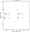 |
Fig. 1. Stretched period échelle diagram for KIC 7458743 obtained from 4-yr Kepler time series. Only peaks with an S/N above eight are shown. The size of the symbols are proportional to the peak amplitude. For clarity, peaks in the vicinity of l = 0 and l = 2 modes are omitted. The échelle diagram is folded with an apparent period spacing of ΔΠ1meas = 76.5 s, which produces the best visual alignment of the ridges. |
2.2. Extraction of mode frequencies
We performed a full seismic analysis of the eight Kepler red giants of our sample. The light curves were taken from Kepler Light Curves Optimized For Asteroseismology (KEPSEISMIC) and downloaded from Mikulski Archive for Space Telescopes (MAST). KEPSEISMIC light curves were corrected from outliers, jumps, and drifts through the implementation of the Kepler Asteroseismic Data Analysis and Calibration Software (KADACS, García et al. 2011). The gaps shorter than 20 days were filled following in-painting techniques described in García et al. (2014) and Pires et al. (2015). The power density spectra (PSD) were then obtained using the Lomb-Scargle periodogram (Lomb 1976; Scargle 1982). The background of the PSD is modeled as a sum of the contributions from the granulation (two Harvey-like profiles, Harvey 1985, with distinct characteristic timescales) and the photon noise (white noise). To obtain an estimate of the background, we fit this model completed with a contribution from the oscillations (modeled as a Gaussian function) to the observed PSD with a maximum likelihood estimation (MLE) method.
To identify significant peaks in the PSD, we searched for peaks that exceed the threshold xp corresponding to a false-alarm probability of p = 0.05 over the whole frequency range where oscillation modes are expected (νmax ± 5 Δν). These peaks can be used to plot stretched échelle diagrams (see Fig. 1). The list of significant modes was then extended to include additional peaks from the PSD that align on the two clear ridges identified in the stretched échelle diagram, while having a power exceeding eight times the background level (see Mosser et al. 2015). Using the identified significant peaks, we obtained a list of guessed frequencies for dipole mixed modes. We then proceeded to fit a model of the oscillation spectrum to the observed PSD. Each mode was modeled as a Lorentzian function with free central frequency νn, l, m, line width Γn, l, m and height Hn, l, m. We used an MLE approach to fit this model to the PSD. The list of measured frequencies are given in Appendix A for all eight stars. The results are shown in the shape of stretched échelle diagrams in Fig. 2. As mentioned above, the ridges are not straight, so that we can only determine an apparent value of the period spacing ΔΠ1meas that provides a rough visual alignment of the ridges. The values of ΔΠ1meas for each star are given in Table 1.
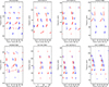 |
Fig. 2. Stretched period échelle diagrams of the eight Kepler red giants of our sample. The échelle diagrams were folded using apparent period spacings ΔΠ1meas that offer good visual alignment of the ridges. To guide the eye, the ridges are highlighted with different colors (red for the most distorted ridge, blue for the other). |
Characteristics of Kepler red giants showing strongly distorted l = 1 doublets.
2.3. Distorted doublets
Figure 2 confirms that the eight stars under study all have l = 1 doublets that show strong distortion in the stretched échelle diagram. For clarity, two distinct colors have been used to highlight the ridges, but at this stage this is only to guide the eye. In the following sections, no assumption has been made about modes belonging to one ridge or the other. Several observations can be made about the stretched échelle diagrams:
-
In all cases the two ridges either cross or get closer to each other in the high-frequency part of the échelle diagram.
-
The intensity of the curvature seems different for the two ridges (in Fig. 2, we represent the ridge showing the strongest curvature in red).
-
The three stars for which the ridges are the most curved (KIC 3326392, KIC 9227589, and KIC 9697268) show hints of mode suppression, the most distorted ridge (the red ridge) vanishing at low frequencies, while the less distorted one (the blue one) remains.
-
There seems to be a difference in mode height between the two ridges. This can be seen by eye for KIC 7458743 in Fig. 1. Our MLE fits confirm that the oscillation modes of the red ridge have heights that are on average 1.9 times larger than those of the blue ridge for this star.
2.4. Location in the Δν − ΔΠ1 plane
Deheuvels et al. (2022) showed that red giants collapse on a clear sequence in the Δν − ΔΠ1 plane (the “degeneracy sequence”) when the electron gas becomes degenerate in the core. The strongly magnetic stars of Deheuvels et al. (2023) had a measured period spacing ΔΠ1meas that was too low, so that these stars appeared below the degeneracy sequence in the Δν − ΔΠ1 plane, where no stars are expected. Accounting for the magnetic field enabled to determine the true period spacing ΔΠ1, which placed these stars back on the degeneracy sequence, as expected (Deheuvels et al. 2023). In Fig. 3, we place our stars in the Δν − ΔΠ1 plane (blue star-shaped symbols) using the apparent period spacing ΔΠ1meas, and their position can be compared to the degeneracy sequence (well identified with the gray crosses). The degeneracy sequence is mass-dependent, higher-mass stars having a lower ΔΠ1 for a given Δν. For each star of the sample, we determined the equation of the degeneracy sequence corresponding to its stellar mass (taken from seismic scaling relations, see Yu et al. 2018). For this purpose, we selected stars among the catalog of Li et al. (2024) that have the same mass within 1σ errors. We fitted a third-degree polynomial to the relation ΔΠ1(Δν) for these stars, giving the degeneracy sequence for the target mass. The difference z between the measured period spacing ΔΠ1meas and the one predicted from the degeneracy sequence is given for each star in Table 1. We find that all our targets are located from 1.6 s to 9.8 s below the degeneracy sequence. The typical scatter around the degeneracy sequence does not exceed 4 s. We thus conclude that six out of eight of our targets can be considered significantly below the degeneracy sequence, confirming the similarity between our targets and those of Deheuvels et al. (2023).
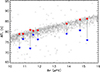 |
Fig. 3. Location of the stars under study in the (Δν-ΔΠ1) plane. The apparent period spacings of g modes ΔΠ1meas are shown as blue star symbols, and the red star symbols indicate the asymptotic period spacing ΔΠ1 measured by accounting for magnetic fields in a non-perturbative manner (Sect. 6). Gray crosses correspond to all red giants studied in Li et al. (2024). |
2.5. Origin of ridge distortion
In Deheuvels et al. (2023), we identified two potential sources for the ridge distortions: buoyancy glitches (corresponding to sharp variations in the profile of the Brunt-Väisälä frequency, with length scales shorter than the mode wavelength), or internal magnetic fields. We ruled out buoyancy glitches, which would produce very different modulation in the ridges (see Appendix A of Deheuvels et al. 2023) and fail to account for the abnormally low measured period spacings. These arguments also hold in the present case. Moreover, with buoyancy glitches, we would expect the two ridges of the doublet to show similar deviations. Indeed, to first order, the modes of each doublet have the same eigenfunctions, so that they should be affected by a buoyancy glitch in the same way. The fact that we observe different curvatures for the two ridges in all our stars makes is even less likely that buoyancy glitches are causing the observed ridge distortion. In the following sections we explore the magnetic hypothesis.
3. Mode identification
If the magnetic field is not axisymmetric (that is, if it does not have an axis of symmetry that coincides with the rotation axis), it splits every l = 1 mode into three components, each of which being also split in three components by the effect of rotation. In principle, a nonaxisymmetric field can thus produce nine components per multiplet (Gough 1990; Loi 2021). Although some of these components are likely to have much smaller amplitudes than the others, we still expect to have more than three components per multiplet if the effects of nonaxisymmetry of the field are nonnegligible. The fact that only two components per multiplet are observed suggests that the nonaxisymmetry effects are indeed weak. We thus discuss the mode identification under this assumption.
3.1. Identification as m = ±1 components
The most natural mode identification for an l = 1 doublet is that we are seeing the m = ±1 components. This occurs when the inclination angle between the rotation axis and the line of sight is close to 90°, that is, the star is seen equator-on. In this case, the m = 0 component geometrically cancels. For a predominantly radial magnetic field, the mode frequencies depends on |m|, so that the m = −1 and m = +1 are affected in the same way by the magnetic field. Only rotational effects can thus produce different curvatures for the two ridges. If the core rotation is slow, the rotational splitting is small and the m = ±1 ridges are nearly parallel, contrary to the observations. A faster core rotation can make the two ridges cross (Gehan et al. 2018), as we observe in most of our stars. However, for all eight stars, we found it impossible to satisfactorily fit the shape of the two ridges and the frequency at which they cross. In Fig. 4, we show the example of KIC 7458743, for which the two ridges cross around a frequency of νcross ≈ 150 μHz. The core rotation needed to produce a crossing of the two ridges at νcross is expressed as ⟨Ω⟩g/(2π) = νcross2ΔΠ1 (Gehan et al. 2018, the presence of a magnetic field is expected to modify this expression, but its effect is negligible for KIC 7458743). This gives a core rotation of ⟨Ω⟩g/(2π)≈1.78 μHz (which would make this star one of the fastest rotators in the Kepler catalog, Li et al. 2024). Using the method that is described in Sect. 6, we fit an asymptotic expression of mixed mode frequencies including the effects of rotation and magnetic fields in a non-perturbative way to one of the observed ridges, taking ⟨Ω⟩g/(2π) = 1.78 μHz. The results are shown in Fig. 4 in a stretched échelle diagram. As can be seen, one of the ridges is very well reproduced, but the second one is completely off. The difference of slopes between the two ridges at the frequency of the crossing is very different in the model and in the observations. If we fit the two ridges simultaneously, considering the core rotation rate and the magnetic field properties as free parameters, the best solution is obtained when the ridges cross around 130 μHz and the quality of the fit is poor. We reach the same conclusion for all eight stars of the sample, we find it impossible to reproduce the observations if we identify the ridges as the m = ±1 components.
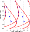 |
Fig. 4. Stretched échelle diagram of KIC 7458743. Filled blue circles show the observed mode frequencies. Open red circles show asymptotic mixed mode frequencies including rotation and magnetic field effects, assuming that the observed ridges correspond to m = ±1 components. The core rotation was determined to ensure a crossing of the ridges at νcross = 150 μHz, and magnetic field properties were adjusted to reproduce the m = −1 ridge (see Sect. 3.1). |
Moreover, the identification as m = ±1 components fails to account for the difference in mode amplitudes between the two ridges, as observed for KIC 7458743 (the m = ±1 components have the same average over the observed disk, so they are expected to have the same amplitude). It does not explain either the suppression of only one of the two ridges, as observed in three stars of the sample (since the magnetic field affects m = ±1 components in the same way, they should be identically suppressed). For all these reasons, we rule out the identification of the ridges as m = ±1 components.
3.2. Identification as m = 0 and m = 1 components
The alternative identification is that one of the two ridges is the m = 0 component. This offers much more flexibility to fit the observed ridges because in general the magnetic field has a different impact on m = 0 and m = ±1 components. The inclination angle between the stellar rotation axis and the line of sight would need to be intermediate, so that both m = 0 and m = 1 components are visible. This configuration could account for the fact that the heights of the two ridges differ in some cases, for example for KIC 7458743. However, it raises the question of why we do not observe three ridges. Two hypotheses can be made to potentially account for this.
First, the core rotation could be too slow to separate the m = ±1 components. This would occur if the core rotation rate is smaller than the typical uncertainties to which mode frequencies can be estimated in the Kepler data. Typically, these uncertainties reach values of about 10 nHz for the most g-like modes near νmax, which is close to the frequency resolution with 4 years of data (νres = 7.9 nHz). In this case, these stars would be exceptionally slow rotators compared to the bulk of Kepler red giants. Indeed, among the 2006 red giants in the catalog of Li et al. (2024), 90% of stars have core rotation rates between 380 nHz and 1170 nHz, and only 8 stars have core rotation rates slower than 100 nHz. This catalog also comprises 489 red giants for which no significant rotational splitting was detected, which can be due to a low inclination angle, but also possibly to a very slow core rotation. One possible explanation for a slow core rotation in our targets would be that the strong internal field produces a very efficient transport of angular momentum that enforces solid-body rotation in the star. We note that near solid-body rotation was found by Li et al. (2024) for six red giants with slow-spinning cores. In Li et al. (2024), envelope rotation rates significantly above zero were measured for only 12% of the catalog (243 stars out of 2006), the other stars having envelope rotation rates compatible with zero. The slowest measured envelope rotation rate is 16 nHz, barely above the frequency resolution. This means that 88% of the stars in the catalog by Li et al. (2024) have envelope rotation below 16 nHz. If a mechanism enforces solid-body rotation in these stars, the core could rotate at rates that are undetectable even with 4 years of Kepler data.
Another possible explanation would be that through a yet unknown mechanism, when the magnetic field becomes near-critical (∼Bc), mode suppression could affect only the m = +1 component or only the m = −1 component. In the following sections, we work under the hypothesis that the two detected ridges correspond to m = 0 and m = 1 components, which is the only way we found of reproducing the observations.
4. Non-perturbative approach
The magnetic fields causing the strong deviation from classical g-mode pattern in our stars are near-critical, so that the effects of magnetic fields on the oscillations need to be addressed with a non-perturbative approach (Rui et al. 2024). Before presenting the details of our non-perturbative approach, adapted from Rui & Fuller (2023) (Sects. 4.2–4.6), we briefly recall a few aspects of the perturbative treatment of magnetic effects on oscillation mode frequencies in Sect. 4.1. This is useful when comparing with the results of the non-perturbative treatment in the next sections.
4.1. Perturbative approach
A perturbative approach was used early on to estimate the effects of a magnetic field on solar p modes (Gough 1990), on g modes in SPB stars (Hasan et al. 2005), and later on mixed modes in red giants, in the special case of a dipolar field with various radial profiles (Gomes & Lopes 2020; Mathis et al. 2021; Bugnet et al. 2021; Loi 2021). Li et al. (2022) generalized the expression of magnetic frequency shifts to magnetic fields with an arbitrary configuration. This study only assumes that the azimuthal field Bφ does not completely dominate over the radial field Br (it is valid provided Bφ/Br ≪ N/ω, where N is the Brunt-Väisälä frequency and ω is the mode angular frequency, with N/ω having typical values on the order of 102 in red giants).
Li et al. (2022) showed that the magnetic frequency shifts depend on only two parameters. The first parameter is the average frequency shift ωB of all the components within the multiplet, which is given by the expression
 (1)
(1)
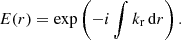
where ℐ is a term depending on the internal structure of the reference model. The term ⟨Br2⟩ is an average of Br2, expressed as
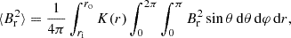 (2)
(2)
where ri and ro are the inner and outer turning points of the g-mode cavity. The weight function, K(r), probes the g-mode cavity and sharply peaks in the H-burning shell. We stress that the average frequency shift ωB strongly increases with decreasing mode frequency (it varies as ω−3). The second parameter that is involved in magnetic frequency shifts is the “asymmetry” parameter aasym, which is a dimensionless quantity that depends on a horizontal average of Br2 weighted by the second-order Legendre polynomial P2(cos θ) and expressed as
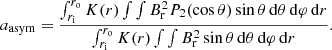 (3)
(3)
Essentially, the parameter ωB gives a measure of the field strength and aasym provides information on the field topology. The average quantity aasym alone can be produced by an infinity of field geometries (Mathis & Bugnet 2023) but its value gives broad constraints on the shape of the field. The parameter aasym indeed ranges between −1/2 (for a field completely concentrated on the equator) and 1 (for a field concentrated at the poles). For a purely dipolar field, aasym takes values between −0.2 and 0.4. Das et al. (2024) showed that having access to magnetic frequency shifts for l = 2 modes could help characterize the field geometry.
If the effects of nonaxisymmetry of the field are negligible (that is, if Br2 is axisymmetric or if the magnetic splitting ωB is smaller than the rotational splitting, see Li et al. 2022), then the magnetic field produces an additional frequency shift to the m = 0 and m = ±1 components, expressed as
 (4)
(4)
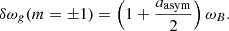 (5)
(5)
In previous works (Li et al. 2022; Deheuvels et al. 2023), ωB was expressed as ωB = δω0(ωmax/ω)3, where δω0 is the average magnetic frequency shift at the frequency of maximum power of the oscillations ωmax.
We attempted to fit expressions given by Eqs. (4) and (5) to the observed mode frequencies of the stars in our sample following the method that was used in Deheuvels et al. (2023), assuming that we detect the m = 0 and m = 1 components with negligible core rotation. For the four stars that show the most strongly curved ridges (KIC 3326392, KIC 5700274, KIC 9227589, and KIC 9697268), no satisfactory solution could be found. We managed to fit either one ridge or the other but not both of them simultaneously. For the other four stars, with less strongly distorted ridges, reasonable fits could be obtained using the perturbative approach. However, the magnetic frequency shift that was measured indicates magnetic fields that are close to the critical field strength, so that a non-perturbative approach is necessary (Rui et al. 2024).
4.2. Non-perturbative approach: Assumptions and analytical problem
We adapted the approach introduced by Rui & Fuller (2023). The authors include the Lorentz force in the oscillation equations using the Boussinesq approximation, which means that the effects of compressibility are taken into account only in the momentum equation. They assume that the oscillations are adiabatic and they make the Cowling approximation, which consists in neglecting the perturbation to the gravitational potential. We make the same assumptions here, also neglecting the effects of rotation in the oscillation equations (even if rotation were to be considered, it could be treated a posteriori as a perturbation because red giants are slow rotators). The magnetic field is assumed to be axisymmetric, which simplifies a lot the equations (the solutions vary as eimφ, with m the azimuthal order). We assume that Bφ/Br ≪ N/ω, so that horizontal field components can be neglected. Finally, the horizontal geometry of Br(r, θ) is assumed to be the same in the whole g-mode cavity, so that it is expressed as Br(r, θ) = B0f(θ)g(r).
For gravity modes, the radial wavenumber is much larger than the horizontal wavenumber (kr/kh ∼ N/ω ∼ 102 in the cores of red giants), so that their displacements are nearly horizontal. Since we consider high-order g modes, the radial wavenumber is also much larger than the length scale of variations of structural quantities. For this reason, Rui & Fuller (2023) adopt the JWKB approximation in the radial direction (but not in the horizontal direction). In the oscillation equations, the eigenfunctions can then be written as the product of a plane-like wave function E(r) and a slowly varying envelope function. For instance, for the pressure perturbation, this yields
 (6)
(6)
The phase function can be expressed as
 (7)
(7)
In the oscillation equations, the radial derivative ∂/∂r can then be replaced by −ikr, which is considered to be much larger than the radial gradients of envelope functions ( ,
,  ...).
...).
Upon making the change of variable μ = cos θ and inserting the equation of motion into the continuity equation (see details in Appendix B), one finds that the pressure perturbation is solution of the eigenvalue problem
 (8)
(8)
where
![Mathematical equation: $$ \begin{aligned} \mathcal{L} \hat{p}&= \frac{\partial }{\partial \mu } \left[ \frac{1-\mu ^2}{1-b^2f^2} \frac{\partial \hat{p}}{\partial \mu } \right] - \frac{m^2}{(1-\mu ^2)(1-b^2f^2)} \hat{p}, \end{aligned} $$](/articles/aa/full_html/2026/05/aa59344-26/aa59344-26-eq11.gif) (9)
(9)
 (10)
(10)
and
 (11)
(11)
In the general case, the coefficients of operator ℒ depend on both r and on μ. Thus the problem cannot be separated into a radial part and a horizontal part. However, with the JWKB approximation, the eigenfunctions of Eq. (8) depend only parametrically on r, as explained in Ogilvie & Lin (2004) (see also Mathis 2009), so that Eq. (8) can be solved in μ for each value of r. It is important to stress that the eigenvalue λ also depends parametrically on r. In the nonmagnetic case (b = 0), Eq. (8) reduces to the general Legendre equation. We then recover λ = l(l + 1) and the horizontal eigenfunctions correspond to the spherical harmonics Ylm(θ, φ).
The quantity b in Eq. (8) has been introduced by Rui & Fuller (2023) as b = krvA, r/ω, where  is the Alfvèn velocity. Because kr ≫ kh, b approximately corresponds to the ratio ωA/ω, where
  is the Alfvèn frequency. The eigenvalue λ can also be written as λ = (b/a)2, where
 (12)
(12)
The quantity a is proportional to the ratio ωsupp2/ω2, where ωsupp is the frequency below which the magnetic field is expected to prevent the propagation of gravity waves (Rui & Fuller 2023). Although the details of how magnetogravity waves are suppressed by the magnetic field remain to be fully understood, it is thought that when they reach the critical frequency ωsupp, these waves refract into outgoing slow magnetic waves that approach infinite wavenumbers and dissipate (Lecoanet et al. 2017; Rui & Fuller 2023; David et al. 2026). Alternately, magnetogravity waves can be damped out by the phase-mixing process when they become resonant with Alfvèn waves (b > 1).
4.3. Profile of the magnetic field
In Rui & Fuller (2023) and Rui et al. (2024), the authors assumed that the field has a dipolar geometry (f(θ) = cos θ). For the radial dependence g(r), they adopted the Prendergast magnetic field geometry (Prendergast 1956). However, it should be noted that Rui et al. (2024) built their Prendergast field by imposing a vanishing surface field. The resulting field slowly decreases as a function of the radius, and it is nearly uniform over the g-mode cavity. Thus, the results presented by the authors approximately correspond to the case g(r) = constant. In this study, we explore different latitudinal and radial dependences for the field. In order to produce different levels of confinement of Br in the core, we assumed a Gaussian-shape profile for g(r) = exp[−r2/(2σB2)]. The parameter σB measures the radial extension of the core field and is considered as a free parameter in our following analysis.
The latitudinal dependence f(θ) of Br is a priori not known. In the perturbative treatment, it intervenes only in the calculation of the asymmetry parameter aasym (Eq. (3)). In this study, we chose to build latitudinal profiles f(θ) that correspond to given values of aasym. Even though the asymmetry parameter does not enter the calculation of magnetic frequency shifts in the non-perturbative approach, it is still interesting to relate f(θ) to aasym because the effects of the magnetic fields on the oscillations are less strong in the high-frequency part of the spectrum, so we expect to approximately recover the solution of the perturbative approach. More importantly, we found that latitudinal profiles corresponding to the same value of aasym produce similar results for all the purposes of our study (see Sect. 5.2 below). Naturally, an infinity of latitudinal profiles produce a given value of aasym. We chose an f(θ) of the type
 (13)
(13)
where δ ∈ ℝ. This is a large-scale field that is antisymmetric with respect to the equator. It has the advantage that it can be made to concentrate near the poles or near the equator depending on the value of δ. Indeed, it can be shown that aasym → 1 for large positive values of δ and aasym → −1/2 for large negative values of δ (despite the fact that the profile vanishes at the equator itself). When plugging the chosen expression of f(θ) in Eq. (3), we find that the function aasym(δ) is continuous and strictly increasing over the interval ] − 1/2, 1[. Thus, for any target aasym, we can find a unique value of δ so that the ratio in Eq. (3) is equal to aasym (see Appendix C.1). We also imposed that the maximum value of |f| is 1. This way, we ensure that the mode becomes suppressed if either a of b exceeds unity somewhere in the star. The multiplication by P1(cos θ) in the expression of f(θ) ensures that ∫0πf(θ)sin(θ) dθ vanishes. In these conditions, the chosen field can be made divergence-free, as expected from Maxwell’s equations, by adding an adequate θ-component Bθ(r, θ) (see Appendix C.3).
4.4. Numerical solution of the horizontal problem
For each radius r, Eq. (8) must be solved numerically. For this purpose, we use a relaxation method. Following Rui & Fuller (2023), we introduce variables 𝒫 = p′/ρ0ω2r2 and  , and the system of equations is then written as
 (14)
(14)
![Mathematical equation: $$ \begin{aligned} \frac{\partial \mathcal{Z} _\theta }{\partial \mu }&= \left( \frac{b^2}{a^2} - \frac{m^2}{(1-\mu ^2)\left[ 1-b^2 f^2(\mu ) \right]} \right) \mathcal{P} . \end{aligned} $$](/articles/aa/full_html/2026/05/aa59344-26/aa59344-26-eq20.gif) (15)
(15)
We started from b = 0 (for which the eigenfunctions correspond to spherical harmonics), and we gradually increased b using the solution from the previous iteration as an initial guess for the next. For each value of b, this procedure provides the eigenfunctions (𝒫 and 𝒵θ) and the parameter a. For a dipole field geometry, Rui & Fuller (2023) showed that a increases with b until the internal gravity wave branch connects with a slow magnetic wave branch, at which point a reaches a maximum value amax. For larger values of b, a then decreases, which shows that the wave propagates back to larger radii inside the star and does not reach the deep core. For an axisymmetric dipolar field (aasym = 0.4), Rui & Fuller (2023) found that in the case (l = 1, m = 0), the maximum value of a is reached when b → ∞ so that the wave is not refracted upward, but reaches infinite wavenumber and dissipates in the layer where a is maximal. In this study, we integrate the equations until either b reaches 1 or a(b) reaches a maximum.
In Fig. 5, we plot the numerical solutions to the horizontal problem obtained with the latitudinal profile given in Eq. (13) and various values of aasym. We plot λ = (b/a)2 as a function of a. For the case aasym = 0.4 corresponding to an axisymmetric dipolar field, we recover the same a(b) relation as Rui & Fuller (2023). For negative asymmetry parameters, we find that λ increases with increasing aasym for a given a, while the situation is reversed for aasym > 0. The cause of mode suppression depends on the value of aasym. The modes become suppressed because of resonance with Alfvèn waves (b exceeds unity) for aasym ≲ −0.204 or aasym ≳ 0.086 with m = 0 modes, and for aasym ≳ 0.464 with m = ±1 modes. For other values of aasym, mode suppression occurs because a reaches amax.
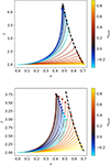 |
Fig. 5. Numerical solution of the horizontal problem for different values of the asymmetry parameter aasym. We show λ as a function of a for (l = 1, m = 0) modes (top panel) and for m = ±1 modes (bottom panel). The colored dots indicate that mode suppression is reached, and the dashed black line corresponds to b = 1. |
4.5. Numerical solution of the radial problem
The JWKB approximation in the radial direction yields the relation
 (16)
(16)
where the expression of kr was taken from Eq. (10). As mentioned above, λ depends parametrically on r, and its value needs to be determined for each layer of the g-mode cavity. For a given field geometry, Eq. (8) can be solved as explained in Sect. 4.4 to obtain a relation between a and b, and thus between a and λ = (b/a)2. This means that λ(r) is known if we can determine a(r) for all radii within the g-mode cavity. The parameter a depends on equilibrium quantities – N(r), ρ(r) – and on the mode frequency ω (see Eq. (12)). Thus to calculate a, we needed a stellar model. The search for a stellar model representative of the studied star is addressed in Sect. 6.2, and here, we assume that we have access to such a model. The dependence of a on ω is an additional complication because the mode frequency is not known at this stage. We therefore proceeded iteratively, initializing ω to its nonmagnetic asymptotic frequency (which is obtained by setting λ = 2 in Eq. (16)) to obtain initial values for a(r). We interpolate the λ(a) relation to determine the value of λ(r) at each radius in the cavity. Equation (16) is then solved to obtain the asymptotic mode frequencies including the effects of the strong field. This process is iterated, the obtained mode frequencies being used to compute updated values of a(r), until convergence. If for some r in the cavity a(r) exceeds amax or b(r) reaches unity, then we consider that the mode is suppressed and it is ignored.
4.6. Example
We here show an example of the oscillation spectrum obtained in the presence of a strong magnetic field. We consider a 1.1-M⊙ stellar model evolved with the evolution code MESA (Paxton et al. 2011) until it reaches a radius of R★ = 5.6 R⊙. We assume a magnetic field Br(r, θ) = B0g(r)f(θ) as explained in Sect. 4.3, setting σB = 0.003 R★ for the radial profile g(r). We choose an asymmetry parameter aasym = 0.34 and build the corresponding function f(θ) (see Appendix C.1). In order to easily compare the results from the perturbative and non-perturbative approaches, it is convenient to relate the field intensity B0 to the magnetic perturbative magnetic frequency shift δω0. In this example, we considered a value of δω0/(2π) = 2.2 μHz, which corresponds to ⟨Br2⟩0.5 = 200 kG. Using Eq. (1), B0 is then obtained as
![Mathematical equation: $$ \begin{aligned} B_0 = \left[ \langle B_{\rm r}^2 \rangle \frac{2}{\int _{r_{\rm i}}^{r_{\rm o}} K(r) g^2(r) \, \mathrm{d}r \, \int _0^\pi f^2(\theta ) \sin \theta \, \mathrm{d}\theta } \right] ^{0.5}. \end{aligned} $$](/articles/aa/full_html/2026/05/aa59344-26/aa59344-26-eq22.gif) (17)
(17)
We then calculated the frequencies of (l = 1, m = 0) and (l = 1, m = 1) modes by solving Eq. (16) (m = ±1 modes have the same frequencies because we ignored rotation here). The results are shown in the shape of a period échelle diagram in the left panel of Fig. 6 (red symbols).
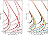 |
Fig. 6. Period échelle diagrams of l = 1 g modes for the example case described in Sect. 4.6. Left: frequencies of m = 0 (circles) and m = 1 (triangles) modes computed for a field with a radial extension σB = 0.003 R★. Magnetic effects are treated either with a non-perturbative approach (red symbols), or a perturbative approach (gray symbols). Right: frequencies of m = 0 modes for values of σ = 0.0015 (red), 0.002 (green), and 0.003 (blue) and for a constant field (black). |
For comparison, we also computed mode frequencies using a perturbative approach as explained in Sect. 4.1 with the same field configuration. The knowledge of δω0/(2π) = 2.2 μHz and aasym = 0.34 uniquely determines the magnetic shifts, given by Eqs. (4) and (5). The results are overplotted in Fig. 6 (gray symbols). As expected, for higher-frequency modes, the magnetic effects are weaker and the mode frequencies from the non-perturbative approach nearly overlap those obtained with the perturbative approach. At lower frequencies, the two sets of frequencies clearly separate and the perturbative approach is no longer valid. Also, evidence of suppression of m = 1 modes is seen at low frequencies.
5. Impact of the profile of Br on mode frequencies
For weak fields, the perturbative approach holds, and the magnetic frequency shifts depend only on weighted averages of the radial field Br in the radial and latitudinal directions (Eq. (2) and (3)). Two different fields producing the same weighted averages are thus expected to have the same impact on mode frequencies. In the non-perturbative approach, the solutions of Eq. (8) depend on the full radial profile g(r) and latitudinal profile f(θ) of Br. This makes the situation more complex, but offers the potential opportunity to constrain the shape of the magnetic field.
5.1. Radial profile of Br
Using the same example case as described in Sect. 4.6 (stellar model and magnetic field configuration), we computed magnetically distorted mode frequencies with different radial extensions of the core field. We considered values of σB of 0.0015 R★, 0.002 R★, and 0.003 R★. For our stellar model, the H-burning shell is located at approximately 6 × 10⁻³ R★ so that the amplitudes of these three fields in the H-burning shell corresponds to 0.04%, 1.3%, and 14.5% of the central amplitude, respectively. Finally, we considered a field that is constant over the whole cavity, similar to the field assumed by Rui & Fuller (2023). For each field, B0 was chosen to produce the same value of ⟨Br2⟩ (Eq. (17)). The left panel of Fig. 7 shows the considered fields. Since the weight function K(r) peaks in the H-burning shell, fields that are confined below this shell have much larger values of B0. The period échelle diagrams of m = 0 modes for these different fields are shown in the right panel of Fig. 6. At higher frequencies, the modes approximately correspond to the perturbative solutions, as expected, but at lower frequencies, it is striking to see that the considered fields produce very different spectra.
 |
Fig. 7. Impact of the radial profile of Br on the mode frequencies. We considered fields with radial extensions of σB = 0.0015 R★ (red lines), 0.002 R★ (green lines), and 0.003 R★ (blue lines) and a constant field (black lines). Left: radial profile of Br. Middle: profile of the parameter a(r) in the g-mode cavity for the mode closest to νmax (Eq. (12)). Right: profile of λ(r) deduced from the interpolation of the a(λ) relation for the same mode (see text). We show the departure from the value λ = 2 corresponding to the perturbative approach. |
The departure from the perturbative solution (gray symbols) is maximal for the constant field. It decreases as σB decreases to reach a minimum for σB ≈ 2 × 10⁻³ R★ and then increases again as σB further decreases. This behavior can be understood from the profile of a(r) and λ(r), which are shown in the middle and right panels of Fig. 7 for the mode that is closest to νmax. The constant field has a maximal amplitude in the H-burning shell where the sensitivity to the field is the highest. It thus has large values of a (and λ values well above two) in this shell, which produces large non-perturbative effects, and causes mode suppression at low-frequency. When the field becomes more confined in the core, the relative amplitude of the field in the H-burning shell decreases, so that non-perturbative effects weaken. For σB = 2 × 10⁻³ R★, the λ value is very close to two in the H-burning shell. Consequently, the ridges are less distorted than in the constant-field case, and mode suppression occurs at much lower frequency (see right panel of Fig. 6). When the field becomes even more confined in the core (σB = 1.5 × 10⁻³ R★), its strength B0 increases to maintain the average ⟨Br2⟩. As a result, the values of a become large at the center, which increases non-perturbative effects and can cause mode suppression. This example demonstrates that measuring the mode frequencies of near-critical fields could give constraints on the radial extent of the core magnetic field, contrary to weaker fields.
5.2. Latitudinal profile of Br
In this study, we found that latitudinal profiles f(θ) producing the same asymmetry parameter aasym lead to very similar magnetic frequency shifts. To reach this conclusion, we considered several different profiles f(θ). Beside the profile given in Eq. (13), we explored profiles of the type f(θ) = P1(cos θ)+BP3(cos θ)+CP5(cos θ). In this expression, B and C can be determined to produce a given value of aasym, although solutions can be found for only a restricted interval (the value C ≈ 2.37 maximizes the reachable range of aasym ∈ [ − 0.252, 0.832]). The value of aasym can also be ensured by profiles of the type  , yielding solutions only over the interval aasym ∈ [ − 0.2, 0.4]. The analyses presented in the following sections of this paper were repeated with the latitudinal profiles presented above, and we found that our results are statistically unchanged. This suggests that non-perturbative effects depend on the latitudinal shape of Br only through the weighted average given by aasym, as for the perturbative approach. In the rest of this study, we used the latitudinal profile given by Eq. (13).
6. Application to red giants with near-critical magnetic fields
We then used the non-perturbative approach described in Sect. 4 to search for strong field configurations that could reproduce the observations for the eight stars of the studied sample. For this purpose, we built an asymptotic expression of mixed modes including the effects of magnetic fields following a non-perturbative approach, and we explored the parameter space.
6.1. Asymptotic model
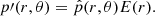
To derive asymptotic expressions of magnetic mixed modes, we followed the approach that was first described in Li et al. (2022) and then used in Li et al. (2023) and Deheuvels et al. (2023). From the work of Shibahashi (1979) and Unno et al. (1989), asymptotic expressions of mixed modes of azimuthal order m are obtained by solving the equation
 (18)
(18)
where q corresponds to the coupling strength between the p- and g-mode cavities, and θp, m, θg, m are phase terms that can be expressed as a function of asymptotic frequencies of p and g modes. Following Mosser et al. (2012c), we have
 (19)
(19)
 (20)
(20)
where Δν(np) and ΔP(ng) are the local large separation of p modes and period spacing of g modes, and νp, m and Pg, m are the frequencies of pure p and periods of pure g modes, respectively1.
The effects of the magnetic field on pressure modes can be neglected (Mathis et al. 2021), and since we considered the case of a negligible rotation, the asymptotic frequencies, νp, m, can be written as
![Mathematical equation: $$ \begin{aligned} \nu _{{p},m} = \left[ n_{\rm p} + \frac{1}{2} + \varepsilon _{\rm p} +\frac{\alpha }{2} \left( n - n_{\rm max} \right)^2 \right] \Delta \nu - d_{01}, \end{aligned} $$](/articles/aa/full_html/2026/05/aa59344-26/aa59344-26-eq27.gif) (21)
(21)
where α measures the second-order effects in the asymptotic development around νmax (as expressed by Mosser et al. 2012c), εp is a phase offset, nmax = νmax/Δν, and d01 corresponds to the small separation δν01 = [νp(0, np)+νp(0, np + 1)−2νp(1, np)]/2 when mode frequencies are expressed at first order.
For g modes, we include the effects of the magnetic field in a non-perturbative way using Eq. (16). For this purpose, a stellar model is needed. This is an additional difficulty compared to the perturbative approach, for which the magnetic shifts only depend on the average quantity ωB (Eqs. (4) and (5)). To explore the parameter space, we computed one reference stellar model for each star (in Sect. 6.2, we explain the choice of a reference model and we discuss the validity of this approach). For this model, we can compute the asymptotic mode frequencies taking into account magnetic fields in a non-perturbative way by solving Eq. (16) for each mode. We can also compute nonmagnetic asymptotic frequencies  by setting λ = 2 in Eq. (16). We then obtain fractional magnetic frequency shifts as
 (22)
(22)
When exploring the parameter space, we assume that the fractional frequency shift of a given mode is that of the reference model given by the expression above. To obtain asymptotic frequencies of pure g modes, we add the magnetic frequency shift given by Eq. (22), leading to the expression
 (23)
(23)
where  .
.
Overall, the free parameters of the asymptotic model are the properties of pure p modes (Δν, εp, α, d01), those of pure g modes (ΔΠ1, εg), the coupling strength q, and the properties of the magnetic field given by the parameters (δω0, σB, aasym). To characterize the field, we proceed as in Sect. 4.6. The free parameters δω0 and σB are used to build the Gaussian-shaped radial profile g(r) of Br (B0 is obtained from δω0 using Eqs. (1) and (17)), and the parameter aasym is used to generate the latitudinal profile f(θ) from Eq. (13). For each set of parameters, the asymptotic frequencies of dipole mixed modes for m = 0 and m = 1 are calculated by solving Eq. (18). Finally, we must remind that asymptotic models are only approximate solutions of the oscillation equations. Departures from asymptotics are taken into account by including a normal model error with widths σp and σg for p and g modes, respectively. The quantities σp and σg are considered as free parameters when searching for optimal solutions.
6.2. Search for reference stellar models
To search for reference models for the eight stars, we used a grid of stellar models computed with MESA (Paxton et al. 2011, 2013, 2015, 2018, 2019), with masses varying between 0.9 and 2 M⊙ (step 0.1 M⊙), metallicities between −0.4 and 0.4 dex (step 0.1 dex), and a step overshoot was added beyond the convective core with αov = 0, 0.1, or 0.2. We used the OPAL equation of state (Rogers & Nayfonov 2002) and opacity tables. We used nuclear reaction rates from NACRE (Angulo et al. 1999). Microscopic diffusion was included by solving the equations of Burgers (1969) at each time step. The models were evolved until they reach 15 R⊙, keeping track of the internal structure for all models computed along the evolution. For each star, we searched for the model of the grid that best reproduces the asymptotic large separation of p modes Δν, the frequency of maximum power of the oscillations νmax, and the asymptotic period spacing of g modes ΔΠ1 by minimizing the function
 (24)
(24)
We note that ΔΠ1 is in fact not known at this stage because the measured period spacing ΔΠ1meas is an underestimated measurement of ΔΠ1 (see Sect. 2.3). To obtain a first estimate of ΔΠ1, we used the results of the perturbative approach obtained in Sect. 4.1. As mentioned above, for the stars with the strongest ridge distortion, this approach cannot fit both ridges simultaneously. In these cases, we used the results of the perturbative approach applied to the ridge showing the weakest distortion alone. We checked a posteriori that it produces estimates of ΔΠ1 that are close to the more proper measurements obtained with the non-perturbative approach in Sect. 6.3.
To check that our conclusions do not critically depend on the choice of a reference model, the fits presented in Sect. 6.3 were performed again using the next best models in the grid and we found that the results were statistically indistinguishable. Similarly, for one of the stars (KIC 5700274), the reference model was updated using the asymptotic period spacing ΔΠ1 found in Sect. 6.3 and a new fit was performed using this model. Again, the posterior distribution of the parameters was found to be nearly identical.
6.3. Asymptotic fits
We fit our model to the observed frequencies by following a Bayesian approach. We used the Asteroseismic Bayesian Inference by MCMC (ABIM) code (see Villate et al. 2026, for more details). ABIM is a Fortran code parallelized with OpenMP directives. Sampling is performed with a Markov Chain Monte Carlo method implementing the so-called stretched move algorithm proposed by Goodman & Weare (2010) and including parallel tempering (e.g., Benomar et al. 2009), which improved the exploration of parameter spaces containing numerous local maxima, as is the case here. We typically sample the posterior distributions with 15 parallel chains and 256 walkers for each chain. The initial positions of the walkers are randomly drawn from the prior distributions. The walkers are iterated over 12 000 steps, with the 2000 first steps discarded as burn-in to ensure that chains are stationary. The priors for each parameter are provided in Appendix D. To calculate the likelihood, we compare each observed mode to the closest mode in the asymptotic model considered.
For each step of the MCMC, we need to compute the relation λ(a) corresponding to the considered value of aasym, which requires solving Eq. (8) using a relaxation scheme, as described in Sect. 4.4. In order to reduce the computing time, we precomputed tables of λ(a) relations for all possible asymmetry parameters with a step of 10−3. Then, during the MCMC procedure, the value of λ is obtained by performing a bilinear interpolation for the considered values of a and aasym.
6.4. Results
For all eight stars, we were able to reproduce very well the observed mode frequencies with our asymptotic model. This can be seen in Fig. 8, which shows stretched échelle diagrams all eight stars We recall that no satisfactory fits had been obtained using a perturbative approach, or identifying the modes as m = ±1 components. We note that the non-perturbative approach as we have applied it in this study involves one more degree of freedom compared to the perturbative approach (the radial extent of the field σB). This increase in the degrees of freedom is fully justified because the perturbative approach (i) fails to fit the most distorted stars, and (ii) leads to field measurements that are close to the critical field strength, which makes the perturbative approach not valid (see Rui et al. 2024).
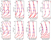 |
Fig. 8. Stretched échelle diagrams of three stars of our sample. Blue circles and horizontal blue lines correspond to observed modes and their 1σ uncertainties. Red empty circles correspond to the best asymptotic models including magnetic effects in a non-perturbative manner. |
The optimal parameters of the asymptotic models are given in Table 2 and we show the posterior probability of a selected sample of parameters in Fig. 9 (see also Figs. D.1 and D.2). In particular, we obtained measurements of the asymptotic period spacing ΔΠ1 that are unbiased by the magnetic field, contrary to the apparent period spacing ΔΠ1meas. We thus revised the location of the eight red giants in the (Δν, ΔΠ1) plane (red star-shaped symbols in Fig. 3). As can be seen in this figure, the stars now clearly belong to the degeneracy sequence, as expected. This result is quite encouraging since we did not include any prior stating that ΔΠ1 should be such that the stars lie on the degeneracy sequence.
 |
Fig. 9. Corner plots of KIC 9227589 (left) and KIC 11408970 (right), restricted to the asymptotic period ΔΠ1 of dipolar g modes, and the parameters characterizing the core magnetic field: the magnetic shift δν0 = δω0/(2π), σB, and aasym. The corner plots for other stars are given in Appendix D. |
Results of fitting asymptotic mode frequencies (including magnetic effects in a non-perturbative way) to the observed frequencies of the red giants in our sample.
6.4.1. Field strength
The measured values of δω0 could be used to obtain estimates of the measured field strength. We expressed them as the weighted average ⟨Br2⟩0.5, for consistency with previous core field measurements. To relate δω0 to ⟨Br2⟩0.5, we used Eq. (1) and the reference stellar models obtained in Sect. 6.2. We accounted for the uncertainties in the measurements of δω0 (Table 2) and uncertainties related to the choice of a reference model were estimated by considering all stellar models from the grid yielding χ2 < χmin2 + 9, where χmin2 is the value of χ2 (see Eq. (24)) for the reference model. We obtained field strengths ranging from about 100–700 kG. These measurements are in line with those found by Deheuvels et al. (2023) for similar stars, except that in this previous study, only lower limits to the field strength were obtained (because only one component per triplet was detected), and a perturbative approach was used even though the fields are near-critical. In the last column of Table 2, we give the value of the field strength at the center B0 for the median model of each star. We find that B0 is always much larger than ⟨Br2⟩0.5. This is because the optimal magnetic fields are all confined well below the H-burning shell (see Sect. 6.4.3). For the four stars that yielded reasonable fits with the perturbative approach (KIC 7458743, KIC 10613561, KIC 10976412, and KIC 11408970), we found that the perturbative approach overestimates the field strength by 5–10%.
In the results presented here, we assumed that the core rotation is too weak to separate m = ±1 components (see Sect. 3.2). Our alternative explanation for the detection of two components only was that for some as-yet-unknown reason, only one of the m = ±1 components is visible. To check the impact of this alternative scenario on our results, we repeated our analysis of one of our stars (KIC 3326392) assuming a core rotation of ⟨Ω⟩g = 0.5 μHz, which is typical for red giants (Hatt et al. 2024; Li et al. 2024). We found that the results are nearly unchanged, the measured field strength being modified by only 10 kG, which is within our quoted uncertainties.
6.4.2. Mode identification
In this study, we assumed that the two detected ridges correspond to m = 0 and m = ±1 ridges, but we made no assumption about which ridge corresponds to which m-component. With the perturbative approach, the nonrotating case holds an ambiguity. The oscillation spectrum corresponding to δω0 and aasym is identical to the spectrum obtained with δω′0 = δω0(2 − aasym)/2 and a′asym = 2aasym/(aasym − 2), the other parameters being unchanged. This degeneracy exists only for aasym < 0.4, to ensure that a′asym ∈ [ − 1/2, 1]. For strong fields, using the non-perturbative approach, this degeneracy is lifted. For all eight stars, the preferred solutions with positive asymmetries are clearly preferred, which corresponds to identifying the most distorted ridge of the m = ±1 component. For some stars, the negative asymmetry solutions appear as a small bump in the posterior distribution of aasym (e.g., for KIC 11408970), but it remains negligible compared to the positive asymmetry solution. This is in line with the observation made for weaker magnetic fields that stars with positive aasym are more frequent that stars with aasym < 0.
6.4.3. Radial extent of the core magnetic field
As demonstrated in Sect. 5.1, we have the possibility to constrain the radial extent of the core magnetic field when the field is near-critical. For all eight stars, we obtained clear contraints on the width σB of the Gaussian function that was used to model the radial profile of Br (see Table 2). The posterior distribution of σB can be seen in the corner plots shown in Figs. 9, D.1, and D.2. For four stars (KIC 5700274, KIC 9227589, KIC 9697268, and KIC 10976412), the posterior distribution of σB peaks on a single value. For KIC 3326392, KIC 10613561, KIC 11408970, and to a lesser extent KIC 7458743, we find a bimodality of the solutions. For instance, for KIC 3326392, the observations can be reproduced either with σB = 0.0018 R★ or with σB = 0.0029 R★. This phenomenon is linked to the behavior described in Sect. 5.1. For a given value of ⟨Br2⟩, non-perturbative effects can be large either when the field is strong near the HBS, or when the field is confined in the central layers. These two possibilities give quite similar oscillation spectra, so that both solutions are possible. In practice, the two solutions lead to similar values of ⟨Br2⟩ and aasym.
For all eight targets, we found that the radial extent of the core field σB is significantly smaller than the radius of the HBS rHBS (the ratio σB/rHBS ranges from 30% to 50% for all eight stars). Consequently, the field strength in the HBS is less than 10% of its maximal intensity for all stars. If we consider magnetic fields that extend closer to the HBS, non-perturbative effects strongly increase, the ridges become too distorted, and mode suppression occurs at too-high frequency compared to the observations, so that no satisfactory solution can be found.
6.4.4. Mode suppression
For KIC 3326392, KIC 9227589, and KIC 9697268, seismic observations have shown that one ridge undergoes mode suppression at low frequency. Even though we did not include as a constraint in our fit that one ridge is suppressed, our best models indeed show mode suppression on the same ridge (the m = ±1 ridge according to Sect. 6.4.2) for all three targets. Moreover, we find that the suppression of the ridge in our optimal models occurs at a frequency that is very close to the lowest-frequency mode detected in the ridge. This can be seen in the stretched échelle diagrams shown in Fig. 8. For KIC 9227589 and KIC 9697268, the lowest-frequency detected mode coincides exactly with the last non-suppressed m = 1 mode in our optimal model. For KIC 3326392, mode suppression occurs at a frequency of 114.83 μHz, which is only slightly higher than the lowest-frequency observed modes (114.41 μHz). We find this agreement quite encouraging, although more thorough work will be needed to determine to what extent the frequency below which modes are suppressed can be used to infer magnetic field properties. We also checked the reason for mode suppression in the three stars. For KIC 9227589 and KIC 9697268, the solution for σB is unimodal and mode suppression occurs because a(r) exceeds the maximal value of amax in the core. For KIC 3326392, the solutions are bimodal, and as could be expected, we find that a(r) exceeds amax in the HBS for the solution with higher σB, and near the core for the solution with lower σB.
7. Discussion
7.1. Origin of the detected fields
One of the main scenarios is that the magnetic fields detected in red giants originate from dynamo action in main-sequence convective cores. Numerical simulations of convective cores in A-type stars show the presence of such fields, with intensities of a few tens of kiloGauss (Brun et al. 2005). After the end of the main sequence, these fields could relax into stable configurations (Becerra et al. 2022), although they might be reshaped by the core contraction (Gouhier et al. 2022). The ohmic diffusion timescale being longer than the star’s lifetime (Cantiello et al. 2016), we expect these fields to survive in the cores of red giants and to remain mostly confined in previously convective layers. As stars evolve in the post-main sequence phase, the HBS progresses outward in mass and eventually outreaches the maximal extent of the convective core during the MS. In this case, the core magnetic field does not extend to the HBS. This reduces the seismically measured field strength ⟨Br2⟩, which has maximal sensitivity near the HBS. This also reduces non-perturbative effects for near-critical fields, as shown in Sect. 5.1, and it corresponds to the configuration that gives best agreement with the seismic observations for our eight targets (Sect. 6.4). The moment when the HBS leaves the previously convective core strongly depends on the stellar mass: it occurs sooner for lower-mass stars (M ∼ 1.2 M⊙), which have small MS convective cores.
Interestingly, we observe that red giants with magnetically distorted doublets tend to have lower masses than other magnetic red giants. Indeed, seven stars (out of eight) have seismic masses that are between 1.12 and 1.24 M⊙, in agreement with the masses of our best-fit models (lying between 1.1 and 1.2 M⊙), while the average seismic mass of magnetic giants detected so far is 1.31 ± 0.15 M⊙ (Li et al. 2022, 2023; Deheuvels et al. 2023; Hatt et al. 2024). The last star, KIC 9697268, has an estimated mass of 1.43 ± 0.09 M⊙ from seismic scaling relations (Yu et al. 2018), but the period spacing ΔΠ1 we measure for this star (see Table 2) makes it more compatible with lower-mass models (our best-fit model has a mass of 1.2 M⊙). For all eight stars, we used our best-fit models to estimate the radius rcc of the layer corresponding to the maximal extent of the convective core during the MS. We found that rcc is below the HBS for all stars (rcc/rHBS is between 40% and 60%). This observation holds regardless of the amount of core overshooting that is added beyond the MS core (rcc varies by only ∼10% when αov is increased from 0 to 0.2). In fact, we find that the radius rcc is remarkably similar to the radial extent of the magnetic field σB that we measured in Sect. 6.4 (the ratio rcc/σB is between 1 and 1.3 for all eight stars). The magnetic fields that we measure for the stars of our sample are thus consistent with the hypothesis that they originate from convective core dynamo.
We note that if our stars were more massive M ≳ 1.4 M⊙, we would be in the inverse situation, the HBS would still be within the layers that were previously convective during the MS. In this case, we have shown that non-perturbative effects are much more severe, and mode suppression occurs at higher frequency. It is therefore tempting to suggest that we are detecting strongly distorted doublets in the stars of our sample precisely because they are low-mass stars, and that more massive stars at the same evolutionary state and with similar field intensity might have lost one or both components to mode suppression. A more thorough search for red giants with near-critical fields could help test this hypothesis.
7.2. Assumptions
We now discuss some of the assumptions that were made in this study.
7.2.1. Radial JWKB approximation in non-perturbative approach
Our non-perturbative approach relies on a number of assumptions, which were already made by Rui & Fuller (2023) and Rui et al. (2024) in their development. The use of a radial JWKB approximation in the unseparated problem would deserve to be validated, ideally using a complete non-perturbative treatment that includes the effects of the magnetic field. This is beyond the scope of this work, but we note that developments pursuing this goal are currently under way (Fort et al. 2024). One of the underlying assumptions is that the radial wavenumber kr introduced in Eq. (7) depends only on r. We investigated this assumption using the ray tracing approach proposed by Loi (2020). The latter study integrates Hamilton’s equations in spherical coordinates using a stellar model and assuming a particular magnetic configuration (a Prendergast field). This procedure gives access to the profile of kr for magnetic fields with arbitrary intensities. We reproduced the approach of Loi (2020) and found that kr remains approximately a function of r only, even for field intensities that approach Bc. This would need to be shown for arbitrary magnetic configurations.
7.2.2. Profile of the magnetic field
In this study, we have assumed that the magnetic field is axisymmetric, mainly because only two components per dipole multiplet are visible. We note that if the core rotation of our stars is indeed very slow, as proposed in Sect. 3.2, then the ratio between the magnetic splitting and the rotational splitting is large. In this case, the alignment of the pulsations is expected to be dictated by the magnetic field rather than the rotation. If the magnetic field possesses an axis of symmetry, then we would indeed be in an axisymmetric configuration along the magnetic axis. So far, non-perturbative treatments of magnetic effects on oscillation mode frequencies were developed under the assumption of an axisymmetric field (Rui & Fuller 2023). When complete non-perturbative calculations are available, it will be interesting to investigate the non-axisymmetric case as well. In this study, we also separated the radial field component into Br(r, θ) = B0f(θ)g(r). This assumption seems reasonable because the oscillation modes are sensitive to the magnetic field only in the g-mode cavity, which has a very small extension in the star (typically ∼1% of the stellar radius) and most of their sensitivity is in the very thin H-burning shell.
8. Conclusion
In this paper, we detected strong deviations from the regular period spacing pattern of g modes in eight Kepler red giants exhibiting l = 1 doublets. The measured period spacings vary with frequency, and they appear abnormally low compared to what is expected for red giant branch stars with strong electron degeneracy in the core (Deheuvels et al. 2022). We ruled out buoyancy glitches as the cause of these features and investigated the magnetic origin. To produce such distortions in the g-mode pattern, the core magnetic field needs to be close to the critical strength, Bc, above which the propagation of magneto-gravity waves is inhibited (Fuller et al. 2015).
We took into account the effects of magnetic fields on oscillation modes using the non-perturbative approach developed by Rui & Fuller (2023) and Rui et al. (2024). We showed that the radial dependence of the radial component of the field Br has a large impact on the intensity of the magnetic frequency shift. This is in contrast with results from the perturbative approach, whereby magnetic frequency shifts only depend on a weighted average of Br2 (Li et al. 2022). This demonstrates that information on the radial profile of Br can be obtained for red giants that host near-critical core magnetic fields. On the contrary, the latitudinal dependence of Br seems to impact magnetic frequency shifts only through the weighted average aasym (Eq. (3)), as in the case of the perturbative approach.
One critical question in our work regards the identification of the two components detected per l = 1 multiplet. If these components are identified as m = ±1, as would be most natural, no satisfactory fit to the data can be found for any of the eight stars. Also, this identification fails to explain the difference of amplitude between the two components in KIC 7458743 or the suppression of one of the two ridges in KIC 3326392, KIC 9227589, and KIC 9697268. As an alternative, we explored the identification of the two components as m = 0 and m = 1. This assumption enabled us to satisfactorily account for all observational features. First, using a non-perturbative approach, we obtained very good fits to the two distorted ridges in all eight stars. Secondly, the period spacings, ΔΠ1, obtained under this assumption brought the eight stars back to the degeneracy sequence where they belong in the (Δν, ΔΠ1) plane (see Fig. 3). Finally, our best-fit solutions for KIC 3326392, KIC 9227589, and KIC 9697268 have a partially suppressed m = 1 ridge, in agreement with the observations, and the frequencies of mode suppression are very close to the observed ones. Despite these successes, it should be noted that we currently cannot satisfactorily explain why only two ridges (and not three) are observed. In this paper, we worked under the assumption that the core rotation is too slow to separate the m = ±1 ridges. So far, magnetic red giants have been found to have a similar core rotation compared to regular red giants (Li et al. 2022; Hatt et al. 2024; Villate et al. 2026). However, the stars studied here have stronger fields than the stars from these previous works, so it is conceivable that in the strong-field regime, the transport of angular momentum could be more efficient. Finally, we note that a toroidal field could act differently on the m = ±1 components (Dhouib et al. 2022), so it would be interesting to investigate the impact of a strong near-critical toroidal field on the oscillations modes of our eight stars in the future.
To reproduce the observations, we had to invoke core magnetic fields, Br, that are confined well below the H-burning shell (Gaussian-shaped profiles for Br with widths σB corresponding to 30–50% of the radius of the HBS). Fields extending all the way to the HBS induce stronger non-perturbative effects so that g-mode period distortion is too large, and mode suppression occurs at too a high frequency to reproduce the observations. If our interpretation is correct, this is the first time we can place constraints on the radial extent of the core magnetic field.
The eight stars under study have a low mass compared to other red giants. Our best-fit stellar models have masses between 1.1 and 1.2 M⊙. They thus had a small convective core during the main sequence. Interestingly, the maximal size of the main-sequence convective core in our models approximately corresponds to our measurements of the radial extent, σB, of the core field. This means that the detected fields could be the remnant of fields generated by a dynamo effect in the main-sequence convective core. More massive stars have larger convective cores so that the HBS is still within the previously convective layers at the bottom of the red giant branch. As we have shown in this paper, non-perturbative effects are stronger in this case and lead to more mode suppression. This might partially explain why the mass distribution of red giants with direct detection of core magnetic fields peaks at a lower mass than the distribution of red giants with suppressed dipolar modes (see Villate et al. 2026). This calls for further investigation.
Acknowledgments
The authors thank the anonymous referee for comments and suggestions that improved the clarity of the manuscript. S.D. and J.B. acknowledge support from from the project BEAMING ANR-18-CE31-0001 of the French National Research Agency (ANR). This work has been supported by CNES, focused on the preparation of the PLATO mission. This paper includes data collected by the Kepler mission and obtained from the MAST data archive at the Space Telescope Science Institute (STScI). Funding for the Kepler mission is provided by the NASA Science Mission Directorate. STScI is operated by the Association of Universities for Research in Astronomy, Inc., under NASA contract NAS 5–26555.
References
- Angulo, C., Arnould, M., Rayet, M., et al. 1999, Nucl. Phys. A, 656, 3 [Google Scholar]
- Aurière, M., Konstantinova-Antova, R., Charbonnel, C., et al. 2015, A&A, 574, A90 [Google Scholar]
- Barrère, P., Guilet, J., Raynaud, R., & Reboul-Salze, A. 2023, MNRAS, 526, L88 [CrossRef] [Google Scholar]
- Becerra, L., Reisenegger, A., Valdivia, J. A., & Gusakov, M. E. 2022, MNRAS, 511, 732 [NASA ADS] [CrossRef] [Google Scholar]
- Beck, P. G., Montalban, J., Kallinger, T., et al. 2012, Nature, 481, 55 [Google Scholar]
- Benomar, O., Appourchaux, T., & Baudin, F. 2009, A&A, 506, 15 [NASA ADS] [CrossRef] [EDP Sciences] [Google Scholar]
- Brun, A. S., Browning, M. K., & Toomre, J. 2005, ApJ, 629, 461 [Google Scholar]
- Bugnet, L. 2022, A&A, 667, A68 [NASA ADS] [CrossRef] [EDP Sciences] [Google Scholar]
- Bugnet, L., Prat, V., Mathis, S., et al. 2021, A&A, 650, A53 [NASA ADS] [CrossRef] [EDP Sciences] [Google Scholar]
- Burgers, J. M. 1969, Flow Equations for Composite Gases (Academic Press) [Google Scholar]
- Cantiello, M., Fuller, J., & Bildsten, L. 2016, ApJ, 824, 14 [NASA ADS] [CrossRef] [Google Scholar]
- Ceillier, T., Eggenberger, P., García, R. A., & Mathis, S. 2013, A&A, 555, A54 [NASA ADS] [CrossRef] [EDP Sciences] [Google Scholar]
- Das, S. B., Einramhof, L., & Bugnet, L. 2024, A&A, 690, A217 [NASA ADS] [CrossRef] [EDP Sciences] [Google Scholar]
- David, C. S., Lecoanet, D., & Garaud, P. 2026, ApJ, 1000, 292 [Google Scholar]
- Deheuvels, S., García, R. A., Chaplin, W. J., et al. 2012, ApJ, 756, 19 [Google Scholar]
- Deheuvels, S., Doğan, G., Goupil, M. J., et al. 2014, A&A, 564, A27 [NASA ADS] [CrossRef] [EDP Sciences] [Google Scholar]
- Deheuvels, S., Ballot, J., Beck, P. G., et al. 2015, A&A, 580, A96 [NASA ADS] [CrossRef] [EDP Sciences] [Google Scholar]
- Deheuvels, S., Ballot, J., Eggenberger, P., et al. 2020, A&A, 641, A117 [EDP Sciences] [Google Scholar]
- Deheuvels, S., Ballot, J., Gehan, C., & Mosser, B. 2022, A&A, 659, A106 [NASA ADS] [CrossRef] [EDP Sciences] [Google Scholar]
- Deheuvels, S., Li, G., Ballot, J., & Lignières, F. 2023, A&A, 670, L16 [NASA ADS] [CrossRef] [EDP Sciences] [Google Scholar]
- Dhouib, H., Mathis, S., Bugnet, L., Van Reeth, T., & Aerts, C. 2022, A&A, 661, A133 [NASA ADS] [CrossRef] [EDP Sciences] [Google Scholar]
- Donati, J. F., & Landstreet, J. D. 2009, ARA&A, 47, 333 [Google Scholar]
- Ferrario, L., de Martino, D., & Gänsicke, B. T. 2015, Space Sci. Rev., 191, 111 [Google Scholar]
- Fort, A., Ouazzani, R. M., & Goupil, M. J. 2024, in SF2A-2024: Proceedings of the Annual meeting of the French Society of Astronomy and Astrophysics, eds. M. Béthermin, K. Baillié, N. Lagarde, et al.. 67 [Google Scholar]
- Fuller, J., Cantiello, M., Stello, D., Garcia, R. A., & Bildsten, L. 2015, Science, 350, 423 [Google Scholar]
- Fuller, J., Piro, A. L., & Jermyn, A. S. 2019, MNRAS, 485, 3661 [NASA ADS] [Google Scholar]
- García, R. A., Hekker, S., Stello, D., et al. 2011, MNRAS, 414, L6 [NASA ADS] [CrossRef] [Google Scholar]
- García, R. A., Ceillier, T., Salabert, D., et al. 2014, A&A, 572, A34 [NASA ADS] [CrossRef] [EDP Sciences] [Google Scholar]
- Gehan, C., Mosser, B., Michel, E., Samadi, R., & Kallinger, T. 2018, A&A, 616, A24 [NASA ADS] [CrossRef] [EDP Sciences] [Google Scholar]
- Gomes, P., & Lopes, I. 2020, MNRAS, 496, 620 [NASA ADS] [CrossRef] [Google Scholar]
- Goodman, J., & Weare, J. 2010, Commun. Appl. Math. Comput. Sci., 5, 65 [Google Scholar]
- Gough, D. O. 1990, in Progress of Seismology of the Sun and Stars, eds. Y. Osaki, & H. Shibahashi (Berlin: Springer Verlag), Lecture Notes in Physics, 367, 283 [Google Scholar]
- Gouhier, B., Jouve, L., & Lignières, F. 2022, A&A, 661, A119 [NASA ADS] [CrossRef] [EDP Sciences] [Google Scholar]
- Harvey, J. 1985, High-resolution helioseismology. Tech. rep. [Google Scholar]
- Hasan, S. S., Zahn, J. P., & Christensen-Dalsgaard, J. 2005, A&A, 444, L29 [NASA ADS] [CrossRef] [EDP Sciences] [Google Scholar]
- Hatt, E. J., Ong, J. M. J., Nielsen, M. B., et al. 2024, MNRAS, 534, 1060 [NASA ADS] [CrossRef] [Google Scholar]
- Jouve, L., Gastine, T., & Lignières, F. 2015, A&A, 575, A106 [NASA ADS] [CrossRef] [EDP Sciences] [Google Scholar]
- Lecoanet, D., Vasil, G. M., Fuller, J., Cantiello, M., & Burns, K. J. 2017, MNRAS, 466, 2181 [Google Scholar]
- Li, G., Deheuvels, S., Ballot, J., & Lignières, F. 2022, Nature, 610, 43 [NASA ADS] [CrossRef] [Google Scholar]
- Li, G., Deheuvels, S., Li, T., Ballot, J., & Lignières, F. 2023, A&A, 680, A26 [NASA ADS] [CrossRef] [EDP Sciences] [Google Scholar]
- Li, G., Deheuvels, S., & Ballot, J. 2024, A&A, 688, A184 [NASA ADS] [CrossRef] [EDP Sciences] [Google Scholar]
- Loi, S. T. 2020, MNRAS, 493, 5726 [CrossRef] [Google Scholar]
- Loi, S. T. 2021, MNRAS, 504, 3711 [NASA ADS] [CrossRef] [Google Scholar]
- Loi, S. T., & Papaloizou, J. C. B. 2017, MNRAS, 467, 3212 [NASA ADS] [Google Scholar]
- Lomb, N. R. 1976, Ap&SS, 39, 447 [Google Scholar]
- Maeder, A., & Meynet, G. 2014, ApJ, 793, 123 [Google Scholar]
- Marques, J. P., Goupil, M. J., Lebreton, Y., et al. 2013, A&A, 549, A74 [NASA ADS] [CrossRef] [EDP Sciences] [Google Scholar]
- Mathis, S. 2009, A&A, 506, 811 [CrossRef] [EDP Sciences] [Google Scholar]
- Mathis, S., & Bugnet, L. 2023, A&A, 676, L9 [NASA ADS] [CrossRef] [EDP Sciences] [Google Scholar]
- Mathis, S., Bugnet, L., Prat, V., et al. 2021, A&A, 647, A122 [EDP Sciences] [Google Scholar]
- Meduri, D. G., Jouve, L., & Lignières, F. 2024, A&A, 683, A12 [NASA ADS] [CrossRef] [EDP Sciences] [Google Scholar]
- Mosser, B., Elsworth, Y., Hekker, S., et al. 2012a, A&A, 537, A30 [NASA ADS] [CrossRef] [EDP Sciences] [Google Scholar]
- Mosser, B., Goupil, M. J., Belkacem, K., et al. 2012b, A&A, 548, A10 [NASA ADS] [CrossRef] [EDP Sciences] [Google Scholar]
- Mosser, B., Goupil, M. J., Belkacem, K., et al. 2012c, A&A, 540, A143 [NASA ADS] [CrossRef] [EDP Sciences] [Google Scholar]
- Mosser, B., Vrard, M., Belkacem, K., Deheuvels, S., & Goupil, M. J. 2015, A&A, 584, A50 [NASA ADS] [CrossRef] [EDP Sciences] [Google Scholar]
- Mosser, B., Pinçon, C., Belkacem, K., Takata, M., & Vrard, M. 2017, A&A, 600, A1 [NASA ADS] [CrossRef] [EDP Sciences] [Google Scholar]
- Mosser, B., Dréau, G., Pinçon, C., et al. 2024, A&A, 681, L20 [NASA ADS] [CrossRef] [EDP Sciences] [Google Scholar]
- Ogilvie, G. I., & Lin, D. N. C. 2004, ApJ, 610, 477 [Google Scholar]
- Paxton, B., Bildsten, L., Dotter, A., et al. 2011, ApJS, 192, 3 [Google Scholar]
- Paxton, B., Cantiello, M., Arras, P., et al. 2013, ApJS, 208, 4 [Google Scholar]
- Paxton, B., Marchant, P., Schwab, J., et al. 2015, ApJS, 220, 15 [Google Scholar]
- Paxton, B., Schwab, J., Bauer, E. B., et al. 2018, ApJS, 234, 34 [NASA ADS] [CrossRef] [Google Scholar]
- Paxton, B., Smolec, R., Schwab, J., et al. 2019, ApJS, 243, 10 [Google Scholar]
- Petitdemange, L., Marcotte, F., & Gissinger, C. 2023, Science, 379, 300 [NASA ADS] [CrossRef] [Google Scholar]
- Pires, S., Mathur, S., García, R. A., et al. 2015, A&A, 574, A18 [NASA ADS] [CrossRef] [EDP Sciences] [Google Scholar]
- Prendergast, K. H. 1956, ApJ, 123, 498 [NASA ADS] [CrossRef] [Google Scholar]
- Raynaud, R., Guilet, J., Janka, H.-T., & Gastine, T. 2020, Sci. Adv., 6, eaay2732 [NASA ADS] [CrossRef] [Google Scholar]
- Rogers, F. J., & Nayfonov, A. 2002, ApJ, 576, 1064 [Google Scholar]
- Rüdiger, G., Gellert, M., Spada, F., & Tereshin, I. 2015, A&A, 573, A80 [NASA ADS] [CrossRef] [EDP Sciences] [Google Scholar]
- Rui, N. Z., & Fuller, J. 2023, MNRAS, 523, 582 [NASA ADS] [CrossRef] [Google Scholar]
- Rui, N. Z., Ong, J. M. J., & Mathis, S. 2024, MNRAS, 527, 6346 [Google Scholar]
- Scargle, J. D. 1982, ApJ, 263, 835 [Google Scholar]
- Shibahashi, H. 1979, PASJ, 31, 87 [NASA ADS] [Google Scholar]
- Spruit, H. C. 2002, A&A, 381, 923 [CrossRef] [EDP Sciences] [Google Scholar]
- Stello, D., Cantiello, M., Fuller, J., et al. 2016, Nature, 529, 364 [Google Scholar]
- Takata, M., Murphy, S. J., Kurtz, D. W., Saio, H., & Shibahashi, H. 2026, MNRAS, 545, staf2153 [Google Scholar]
- Tayler, R. J. 1973, MNRAS, 161, 365 [CrossRef] [Google Scholar]
- Thompson, C., & Duncan, R. C. 1993, ApJ, 408, 194 [NASA ADS] [CrossRef] [Google Scholar]
- Unno, W., Osaki, Y., Ando, H., Saio, H., & Shibahashi, H. 1989, Nonradial Oscillations of Stars (Tokyo: University of Tokyo Press) [Google Scholar]
- Vidotto, A. A., Gregory, S. G., Jardine, M., et al. 2014, MNRAS, 441, 2361 [Google Scholar]
- Villate, M., Deheuvels, S., & Ballot, J. 2026, A&A, 707, A366 [NASA ADS] [CrossRef] [EDP Sciences] [Google Scholar]
- Villebrun, F., Alecian, E., Hussain, G., et al. 2019, A&A, 622, A72 [NASA ADS] [CrossRef] [EDP Sciences] [Google Scholar]
- Yu, J., Huber, D., Bedding, T. R., et al. 2018, ApJS, 236, 42 [NASA ADS] [CrossRef] [Google Scholar]
As mentioned in Villate et al. (2026), the expression of θg, m was modified compared to Mosser et al. (2015), so that we recover the frequencies of pure g modes as solutions of Eq. (18) when the coupling parameter q tends to zero.
Appendix A: Mode frequencies
We give the measured mode frequencies for all eight stars of the sample as obtained from our maximum likelihood estimation technique (see Sect. 2.2) in Tables A.1 and A.2.
Frequencies of l = 0 and l = 1 detected oscillation modes for KIC 3326392, KIC 5700274, KIC 7458743, and KIC 9227589.
Frequencies of l = 0 and l = 1 detected oscillation modes for KIC 9697268, KIC 10613561, KIC 10976412, and KIC 11408970.
Appendix B: Oscillation equations in non-perturbative framework
We here detail the main steps that lead to the expressions for g mode frequencies with magnetic field taken into account in a non-perturbative manner. The development essentially follows that of Rui & Fuller (2023). With the assumptions made in Sect. 4.2, the oscillation equations can be written as follows. The continuity equation reads:
 (B.1)
(B.1)
The momentum equations are written as:
 (B.2)
(B.2)
 (B.3)
(B.3)
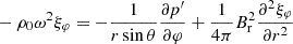 (B.4)
(B.4)
We assume the oscillations are adiabatic, so the energy equation can be replaced by the adiabaticity relation
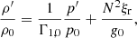 (B.5)
(B.5)
where Γ1, 0 is the adiabatic index. For gravity waves, the first term in the right-hand-side of Eq. (B.5) can be neglected, so that ρ′≃ρ0N2ξr/g0.
All the eigenfunctions are written as the product of a plane-like wave function E(r) = exp(−i∫kr dr) and an envelope function (for instance  for the pressure perturbation) that is a slowly varying function of the radius. The continuity equation then becomes
 (B.6)
(B.6)
Combining the radial equation of motion with the adiabaticity relation, we obtain
 (B.7)
(B.7)
Since ω ≪ N, the left-hand term of this equation can be neglected. The horizontal equations of motion yield
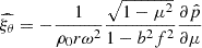 (B.8)
(B.8)
 (B.9)
(B.9)
We insert these expressions into the continuity equation, yielding
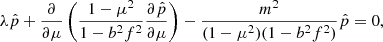 (B.10)
where
 (B.11)
Appendix C: Magnetic field profile
C.1. Latitudinal profile of Br
To build the latitudinal profile f(θ) introduced in Eq. (13), we need to determine the value of δ corresponding to a given aasym = ∫−11f2P2dμ/∫−11f2dμ. The denominator can be expressed as I1e−δ, where
 (C.1)
(C.1)
To calculate these integrals numerically, we express them as:
 (C.2)
(C.2)
and terms in the summation are added until they become smaller than 10−15. The numerator can be written as e−δ(3I2 − I1)/2, so that
 (C.3)
(C.3)
The value of δ corresponding to a given aasym is obtained by using a Newton-Raphson algorithm and making use of the following expression for the derivative daasym/dδ:
 (C.4)
(C.4)
C.2. Alternative expression for f(θ)
We can also build a latitudinal profile f(θ) for the radial field Br in the shape f(θ) = P1(cos θ)+BP3(cos θ)+CP5(cos θ). For a given value of the asymmetry parameter aasym, the field must satisfy Eq. (3). This is achieved provided
 (C.5)
(C.5)
We find that the value C ≈ 2.37 maximizes the interval of asymmetry parameters that are reachable. Solutions to the previous equation can be found for −0.252 ≲ aasym ≲ 0.832. This does not cover the full range of possible values for aasym, but gives satisfactory coverage for this study at least for the solutions with positive asymmetries. We then divide the obtained profile f(θ) by is maximum absolute value to satisfy the condition max(|f|) = 1.
C.3. Making the field divergence-free
We need to ensure that the magnetic field that we build satisfies the condition ∇ · B = 0. The field is axisymmetric, so that the azimuthal component Bφ(r, θ) can be arbitrarily chosen without affecting the divergence of B. We add a θ-component Bθ(r, θ) in such a way that
 (C.6)
(C.6)
This is achieved if Bθ takes the form
![Mathematical equation: $$ \begin{aligned} B_{\theta }(r,\theta ) = - \frac{B_0}{r} \frac{\mathrm{d}}{\mathrm{d}r}\left[ r^2 g(r) \right] \frac{\int _0^\theta f(\theta \prime )\sin \theta \prime \,\mathrm{d}\theta \prime }{\sin \theta } \end{aligned} $$](/articles/aa/full_html/2026/05/aa59344-26/aa59344-26-eq86.gif) (C.7)
(C.7)
This solution is regular at the poles (μ = cos θ → ±1). Indeed, by expending μ = ±(1 − ε), one finds that the numerator is equivalent to eδε while the denominator varies as  .
.
Appendix D: Priors and results for ABIM
D.1. Priors
When using the ABIM code to fit asymptotic expressions of mixed modes (including effects from rotation and magnetic fields) to the observations (Sect. 6.3), we impose a set of priors on the free parameters. The priors are chosen either uniform (U) over a range [xmin, xmax], “uniform-periodic” (UP), which is a uniform distribution for a periodic parameter (the steps of the walkers are calculated modulo the period), or “uniform-normal” (UG), which is a uniform distribution with Gaussian tails at the edges (σmin and σmax are the widths of the tails at both ends).
Our choices for the priors are summarized in Table D.1. For the large separation Δν, we used a uniform prior centered on the value measured by Yu et al. (2018) with an interval of ±1 μHz. The phase terms εp and εg have a periodicity of one. The priors on α and d01 were designed based on measurements of these parameters for other similar red giants. The uniform prior on the period spacing ΔΠ1 was chosen to include the apparent period spacing ΔΠ1meas (which is lower than the expected value) and extend 6 s above the degeneracy sequence (Deheuvels et al. 2022). For the coupling strength q, we chose a uniform distribution ranging up to 0.2, which covers the expected values on the red giant branch. The uniform prior on the magnetic frequency shift δν0 (which is related to the quantity ⟨Br2⟩) was chosen to extend well beyond the values measured by Deheuvels et al. (2023). The asymmetry parameter aasym takes values between −0.5 and 1, which are in principle all reachable by the latitudinal profile that we chose (Eq. (13)). However, we must have δ → ±∞ to reach the edges of this range, which causes numerical problems. For this reason, we restricted the prior distribution to [ − 0.45, 0.9]. The radial extension of the field is parametrized by σB, for which we chose a uniform prior distribution in the range [0.001, 0.009] R★. The upper limit of this interval corresponds to a field that is nearly constant within the g-mode cavity. Finally, the priors on σp and σg, which characterize the model errors, were chosen based on model errors computed for the red giants studied in Li et al. (2024).
Choice of priors for ABIM.
D.2. Corner plots
In Fig. D.1 and D.1, we show corner plots similar to those of Fig. 9 for KIC 3326392, KIC 5700274, KIC 7458743, KIC 9697268, KIC 10976412, and KIC 11408970. For clarity, the corner plots are restricted to the asymptotic period ΔΠ1 of dipolar g modes, and the parameters characterizing the core magnetic field: the magnetic shift δν0 = δω0/(2π), σB, and aasym.
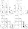 |
Fig. D.2. Same as Fig. 9 for KIC 7458743 (top left), and KIC 9697268 (top right), KIC 10613561 (bottom left) and KIC 10976412 (bottom right). |
All Tables
Results of fitting asymptotic mode frequencies (including magnetic effects in a non-perturbative way) to the observed frequencies of the red giants in our sample.
Frequencies of l = 0 and l = 1 detected oscillation modes for KIC 3326392, KIC 5700274, KIC 7458743, and KIC 9227589.
Frequencies of l = 0 and l = 1 detected oscillation modes for KIC 9697268, KIC 10613561, KIC 10976412, and KIC 11408970.
All Figures
|
Fig. 1. Stretched period échelle diagram for KIC 7458743 obtained from 4-yr Kepler time series. Only peaks with an S/N above eight are shown. The size of the symbols are proportional to the peak amplitude. For clarity, peaks in the vicinity of l = 0 and l = 2 modes are omitted. The échelle diagram is folded with an apparent period spacing of ΔΠ1meas = 76.5 s, which produces the best visual alignment of the ridges. |
| In the text | |
|
Fig. 2. Stretched period échelle diagrams of the eight Kepler red giants of our sample. The échelle diagrams were folded using apparent period spacings ΔΠ1meas that offer good visual alignment of the ridges. To guide the eye, the ridges are highlighted with different colors (red for the most distorted ridge, blue for the other). |
| In the text | |
|
Fig. 3. Location of the stars under study in the (Δν-ΔΠ1) plane. The apparent period spacings of g modes ΔΠ1meas are shown as blue star symbols, and the red star symbols indicate the asymptotic period spacing ΔΠ1 measured by accounting for magnetic fields in a non-perturbative manner (Sect. 6). Gray crosses correspond to all red giants studied in Li et al. (2024). |
| In the text | |
|
Fig. 4. Stretched échelle diagram of KIC 7458743. Filled blue circles show the observed mode frequencies. Open red circles show asymptotic mixed mode frequencies including rotation and magnetic field effects, assuming that the observed ridges correspond to m = ±1 components. The core rotation was determined to ensure a crossing of the ridges at νcross = 150 μHz, and magnetic field properties were adjusted to reproduce the m = −1 ridge (see Sect. 3.1). |
| In the text | |
|
Fig. 5. Numerical solution of the horizontal problem for different values of the asymmetry parameter aasym. We show λ as a function of a for (l = 1, m = 0) modes (top panel) and for m = ±1 modes (bottom panel). The colored dots indicate that mode suppression is reached, and the dashed black line corresponds to b = 1. |
| In the text | |
|
Fig. 6. Period échelle diagrams of l = 1 g modes for the example case described in Sect. 4.6. Left: frequencies of m = 0 (circles) and m = 1 (triangles) modes computed for a field with a radial extension σB = 0.003 R★. Magnetic effects are treated either with a non-perturbative approach (red symbols), or a perturbative approach (gray symbols). Right: frequencies of m = 0 modes for values of σ = 0.0015 (red), 0.002 (green), and 0.003 (blue) and for a constant field (black). |
| In the text | |
|
Fig. 7. Impact of the radial profile of Br on the mode frequencies. We considered fields with radial extensions of σB = 0.0015 R★ (red lines), 0.002 R★ (green lines), and 0.003 R★ (blue lines) and a constant field (black lines). Left: radial profile of Br. Middle: profile of the parameter a(r) in the g-mode cavity for the mode closest to νmax (Eq. (12)). Right: profile of λ(r) deduced from the interpolation of the a(λ) relation for the same mode (see text). We show the departure from the value λ = 2 corresponding to the perturbative approach. |
| In the text | |
|
Fig. 8. Stretched échelle diagrams of three stars of our sample. Blue circles and horizontal blue lines correspond to observed modes and their 1σ uncertainties. Red empty circles correspond to the best asymptotic models including magnetic effects in a non-perturbative manner. |
| In the text | |
|
Fig. 9. Corner plots of KIC 9227589 (left) and KIC 11408970 (right), restricted to the asymptotic period ΔΠ1 of dipolar g modes, and the parameters characterizing the core magnetic field: the magnetic shift δν0 = δω0/(2π), σB, and aasym. The corner plots for other stars are given in Appendix D. |
| In the text | |
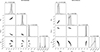 |
Fig. D.1. Same as Fig. 9 for KIC 3326392 (left) and KIC 5700274 (right). |
| In the text | |
|
Fig. D.2. Same as Fig. 9 for KIC 7458743 (top left), and KIC 9697268 (top right), KIC 10613561 (bottom left) and KIC 10976412 (bottom right). |
| In the text | |
Current usage metrics show cumulative count of Article Views (full-text article views including HTML views, PDF and ePub downloads, according to the available data) and Abstracts Views on Vision4Press platform.
Data correspond to usage on the plateform after 2015. The current usage metrics is available 48-96 hours after online publication and is updated daily on week days.
Initial download of the metrics may take a while.