© The Authors 2026

1 Introduction

The Fermi Large Area Telescope (LAT, Atwood et al. 2009) dataset contains a near-continuous all-sky history of the arrival times of gamma-ray photons detected since Fermi’s launch in 2008. Significant pulsations from more than 300 pulsars have been detected in the LAT data (Smith et al. 2023), split nearly evenly between energetic young pulsars and rapidly spinning recycled millisecond pulsars (MSPs).

While pulsar timing studies, in which models for pulse arrival times are built to keep track of pulsar rotations, have long been applied to radio pulsar observations, a wealth of astrophysical processes can also be probed by timing gamma-ray pulsations in the LAT data. In fact, around 80 pulsars can only be reliably timed in gamma-ray data (Smith et al. 2023), either because they appear to be radio quiet (e.g. Abdo et al. 2009; Pletsch et al. 2012b) or because their radio pulses are nearly always eclipsed by intra-binary material (Ray et al. 2013, 2020; Nieder et al. 2020; Thongmeearkom et al. 2024). Although they are a minor fraction of the total pulsar population, these pulsars represent some of the most energetic and most compact binaries, respectively. Furthermore, the LAT data allows pulsars to be timed retroactively after their discovery, which provides an immediate multi-year timing baseline, something that is only possible in radio data for a small number of special sky locations with multiple archival observations, for example globular clusters (Balakrishnan et al. 2023; Padmanabh et al. 2024).

The characterisation of timing noise (TN; stochastic variations in rotational frequency, see e.g. Kerr et al. 2015), glitches (sudden, instantaneous jumps in frequency, see e.g. Pletsch et al. 2012a; Panin & Sokolova 2025), and correlated variability between spin-down rate and flux (Allafort et al. 2013; Takata et al. 2020; Fiori et al. 2024) in young gamma-ray pulsars can probe the dynamic pulsar magnetosphere and neutron star structure. Gamma-ray timing of binary MSPs has shown that complicated orbital period variations are nearly universal in redback binary systems (e.g. Pletsch & Clark 2015; Thongmeearkom et al. 2024), and has revealed a possible planetary-mass tertiary in one system (Nieder et al. 2022). The construction of a gamma-ray pulsar timing array (GPTA) could also provide an important cross-check of the searches for and characterisation of the stochastic gravitational wave background (GWB) from radio pulsar timing array (PTA) projects (The Fermi-LAT Collaboration 2022, hereafter GPTA Paper I). While the GPTA is less sensitive than radio PTAs, it is immune to variations in the interstellar medium, which disperses and scatters radio pulsations and can thereby bias radio timing models.

While sophisticated radio pulsar timing methods and models have been developed (e.g. Lentati et al. 2014; Ellis et al. 2020; Susobhanan 2025), particularly for PTA experiments, these are often not applicable to gamma-ray data, which means dedicated gamma-ray timing methods have to be developed to make the most of this dataset. In the first gamma-ray timing studies (Ray et al. 2011; Kerr et al. 2015), several weeks or months of gamma-ray data were integrated to produce statistically significant integrated pulse profiles. These could then be compared to a template pulse to extract a small number of times-of-arrival (ToAs) that could be analysed using existing radio pulsar timing tools. However, many gamma-ray pulsars are faint enough that the required ToA integration timescales are longer than those of important timing effects such as binary Doppler shifts, or variations in the Solar-System R0mer delay, meaning binary and astrometry parameters must be assumed in advance and cannot then be fit from the extracted ToAs. This procedure also assigns a symmetrical Gaussian uncertainty to each ToA, an assumption that may not be accurate when the pulsation signal-to-noise ratio is low.

Later works (e.g. Pletsch & Clark 2015; Clark et al. 2015) developed a fully un-binned approach that optimises the Poisson likelihood for the observed photon arrival times, given an assumed pulse profile shape. This technique was then further extended to also marginalise over the uncertain shape of the pulse profile (Nieder et al. 2019) by sampling the parameters describing the template pulse profile alongside the timing model. This method uses the information from every individual photon arrival time, allowing all binary and astrometric parameters to be fit to the data. However, it requires a multi-dimensional Markov chain Monte Carlo (MCMC) sampling process that can become inefficient as the number of timing model parameters increases, and was not able to fit for stochastic noise components. In GPTA Paper I, a similar un-binned photon-by-photon timing approach was used, where a Gaussian approximation to the timing model likelihood was assumed. This does enable the estimation of TN properties for gamma-ray MSPs, but assumes a fixed pulse profile template.

In this paper, we present a new method that extends the Gaussian process framework commonly used in radio pulsar timing to the gamma-ray data, allowing for the efficient fitting of even complicated timing models, and a robust estimation of stochastic noise processes, while accounting for uncertainty in the template pulse profile. We implemented this method in a python package called shoogle¹,², which uses the PINT pulsar timing package (Luo et al. 2021 ; Susobhanan et al. 2024) to evaluate the pulsar timing model and its derivatives, and the JAX (Bradbury et al. 2018) and BlackJAX (Cabezas et al. 2024) python libraries for GPU-acceleration and efficient sampling.

This paper is organised as follows. Section 2 describes our new method (with notation summarised in Table A.1). It begins with a summary of how the Gaussian process framework is used in pulsar timing (Section 2.1); presents the gamma-ray timing problem (Section 2.2) and our new method for tackling it (Section 2.3); and describes how this method can be used to time orbital period variations in spider binary systems (Section 2.4), the problem that was our original motivation for developing this method. In Section 3 we test the method on both real and simulated pulsar data, and demonstrate its accuracy. In Section 4, we discuss further possible uses for and extensions to this method, before briefly summarising in Section 5.

2 Methods

2.1 Pulsar timing using Gaussian processes

Pulsar timing analyses consist of finding a set of parameters ρ for a timing model Φ(t, ρ) that minimise the variance of the rotational phases for a set of observed pulse ToAs t. Often this consists in a constant spin-down model,

$$\mathrm{\Phi }(t,\rho \mathbf{)}\mathbf{=}(\mathbf{f}{\mathbf{t}}_{\mathrm{p}\mathrm{s}\mathrm{r}}\mathbf{(}\mathbf{t}\mathbf{,}\rho \mathbf{)}\mathbf{+}\frac{\mathbf{1}}{\mathbf{2}}\dot{\mathbf{f}}{\mathbf{t}}_{\mathrm{p}\mathrm{s}\mathrm{r}}\mathbf{(}\mathbf{t}\mathbf{,}\rho {\mathbf{)}}^{\mathbf{2}})mod\mathbf{1}\mathbf{,}$$(1)

where f is the pulsar spin frequency, f is the spin-down rate, and t_psr is the time at which a pulse detected at time t was emitted by the pulsar (up to an arbitrary constant), taking into account various delays (Edwards et al. 2006): light travel time R0mer delays due to the pulsar’s location in a binary system, and due to Earth’s motion around the solar-system; radio propagation delays; and relativistic delays due to light propagation through curved spacetime. All of these delays are unknown in advance, and must be parameterised and estimated from the data.

Pulsar timing analyses usually make two approximations. First, the timing model is approximated as a linear expansion with parameter offsets θ ≡ ρ - ρ₀, relative to the initial model parameters ρ₀,

$$\mathbf{\Phi }\mathbf{(}\mathbf{t}\mathbf{,}\rho \mathbf{)}\approx \varphi \mathbf{(}\mathbf{t}\mathbf{,}\theta \mathbf{)}\equiv {\varphi }_{\mathbf{0}}\mathbf{(}\mathbf{t}\mathbf{)}\mathbf{-}\mathbf{M}\mathbf{(}\mathbf{t}\mathbf{)}\theta \mathbf{,}$$(2)

where φ₀(t) ≡ Φ(t, ρ₀) are the pre-fit spin phases according to the initial model, and M(t) is the design matrix, containing the derivatives of the phase model at the observed arrival times, with respect to the parameters:

$$M_{ij}(\mathbf{t}\mathbf{)}\mathbf{=}{\frac{\mathrm{\partial }\mathbf{\Phi }\mathbf{(}{\mathbf{t}}_{\mathbf{i}}\mathbf{,}\rho \mathbf{)}}{\mathrm{\partial }{\rho }_{\mathbf{j}}}|}_{\rho \mathbf{=}{\rho }_{\mathbf{0}}}\mathbf{.}$$(3)

This linear approximation is exact for some parameters, although not all (Susobhanan 2025), but is generally a good approximation around the best-fitting models. For brevity, we shall drop the explicit dependences of φ and M on t and θ hereafter.

The second approximation that is nearly universally assumed is that the likelihood function for the data, D (which consists of the ToAs, t, and their uncertainties, σ) is approximated as a multivariate Gaussian, with log-likelihood:

$$\log p(D\mid \theta )=-\frac{1}{\text{2}}[\log \left|2\pi C\right|+{({\varphi }_{\mathbf{0}}\mathbf{-}\mathbf{M}\theta )}^T{C}^{-1}({\varphi }_{\mathbf{0}}\mathbf{-}\mathbf{M}\theta )],$$(4)

where C is the data covariance matrix. In the simplest case, this matrix contains (fσ)² along its diagonal, assuming all ToAs are independent of one another. However, it can also contain off-diagonal elements to account for instrumental effects that introduce correlations between observations.

This Gaussian likelihood assumption is an excellent approximation for radio data, where the arrival time and a precise Gaussian uncertainty of a nominal pulse can be obtained by cross-correlating the (usually high S/N) folded data from an observation against a template pulse profile.

With these simplifying assumptions, the timing model fit follows simple generalised least squares. The above log-likelihood can be re-arranged to

$$\begin{array}{rl}\log p(D\mid \theta )=-\frac{1}{\text{2}}[& \log \left|2\pi C\right|+{\varphi }_{\mathbf{0}}^{\mathbf{T}}{\mathbf{C}}^{\mathbf{-}\mathbf{1}}{\varphi }_{\mathbf{0}}\mathbf{-}{\hat{\theta }}^{\mathbf{T}}{\mathbf{\Sigma }}^{\mathbf{-}\mathbf{1}}\hat{\theta }\\ & +{(\theta \mathbf{-}\hat{\theta })}^T{\mathrm{\Sigma }}^{-1}(\theta \mathbf{-}\hat{\theta })],\end{array}$$(5)

showing that this is also a multivariate Gaussian in θ, with maximum-likelihood estimator θ and covariance matrix Σ

$$\begin{array}{rl}\mathrm{\Sigma }& ={\left(M^T{C}^{-1}M\right)}^{-1},\\ \hat{\theta }& =\mathrm{\Sigma }{M}^T{C}^{-1}{\varphi }_{\mathbf{0}}\mathbf{.}\end{array}$$(6)

Modern radio pulsar timing analyses have timing models with components that account for seemingly stochastic signals or sources of correlated noise: intrinsic red noise in the pulsar’s spin rate (Coles et al. 2011); time-dependent variations in the dispersion measure (Larsen et al. 2024; Iraci et al. 2024); variations in the density of the Solar wind (Susarla et al. 2024); and the GWB (van Haasteren et al. 2009; Lentati et al. 2013). Obtaining robust estimates of the properties of these processes can be crucial, either because the processes themselves are the scientific target (e.g. measuring the amplitude and spectrum of the GWB), or because these processes must be accounted for to obtain robust estimates for other timing properties of interest (Coles et al. 2011).

This can be achieved by treating these effects as stochastic Gaussian processes, which have been extensively studied in the literature. An exact solution would be obtained by simply modifying the data covariance matrix, C, to reflect the expected correlations in the residuals due to these noise components. However, this can be expensive, as the cost of inverting C grows with the cube of the number of ToAs.

Instead, in the pulsar timing framework, these Gaussian processes are normally fit using a low-rank approximation (van Haasteren & Vallisneri 2015). This is done by including a set of basis vectors in M for each noise component, with corresponding coefficients in θ that have a Gaussian prior whose variance is determined by a set of hyper-parameters, λ, quantifying these noise processes. In pulsar timing analyses, these basis vectors are usually chosen to be a Fourier-series expansion, in which case the hyperparameters describe a model power spectral density (PSD) that defines the prior variance on the Fourier amplitudes, although it has been shown recently that a sparse time-domain basis yields more accurate results (Crisostomi et al. 2025).

For a Gaussian prior on θ, centred on θ₀ and with covariance matrix Λ(λ), the posterior distribution for θ,

$$\log p(\theta \mid \mathbf{D}\mathbf{,}\lambda )=\log p(D\mid \theta )+\log p(\theta \mid \lambda )-\log p(D\mid \lambda ),$$(7)

is

$$\begin{array}{rl}\log p(\theta \mid \mathbf{D}\mathbf{,}\lambda )=-\frac{1}{\text{2}}[& \log \left|2\pi C\right|+{\varphi }_{\mathbf{0}}^{\mathbf{T}}{\mathbf{C}}^{\mathbf{-}\mathbf{1}}{\varphi }_{\mathbf{0}}\mathbf{-}{\hat{\theta }}^{\mathbf{T}}{\mathbf{\Sigma }}^{\mathbf{-}\mathbf{1}}\hat{\theta }\\ & +{(\theta \mathbf{-}\hat{\theta })}^T{\mathrm{\Sigma }}^{-1}(\theta \mathbf{-}\hat{\theta })\\ & +\log \left|2\pi \mathrm{\Lambda }\right|+{(\theta \mathbf{-}{\theta }_{\mathbf{0}})}^T{\mathrm{\Lambda }}^{-1}(\theta \mathbf{-}{\theta }_{\mathbf{0}})]\\ & -\log p(D\mid \lambda ).\end{array}$$(8)

Expanding the quadratics and completing the square in θ shows that the posterior distribution on θ given λ follows another multivariate Gaussian in θ:

$$\begin{array}{rl}\log p(\theta \mid \mathbf{D}\mathbf{,}\lambda )=-\frac{1}{\text{2}}[& \log \left|2\pi C\right|+\log \left|2\pi \mathrm{\Lambda }\right|\\ & +{\varphi }_{\mathbf{0}}^{\mathbf{T}}{\mathbf{C}}^{\mathbf{-}\mathbf{1}}{\varphi }_{\mathbf{0}}\mathbf{+}{\theta }_{\mathbf{0}}^{\mathbf{T}}{\mathbf{\Lambda }}^{\mathbf{-}\mathbf{1}}{\theta }_{\mathbf{0}}\mathbf{-}{\overline{\theta }}^{\mathbf{T}}{\mathbf{\Gamma }}^{\mathbf{-}\mathbf{1}}\overline{\theta }\\ & +{(\theta \mathbf{-}\overline{\theta })}^T{\mathrm{\Gamma }}^{-1}(\theta \mathbf{-}\overline{\theta })]\\ & -\log p(D\mid \lambda ),\end{array}$$(9)

with the new covariance matrix and mean

$$\begin{array}{rl}\mathrm{\Gamma }& ={({\mathrm{\Sigma }}^{-1}+{\mathrm{\Lambda }}^{-1})}^{-1},\\ \overline{\theta }& =\mathrm{\Gamma }({\mathrm{\Sigma }}^{-1}\hat{\theta }+{\mathrm{\Lambda }}^{-1}{\theta }_{\mathbf{0}}).\end{array}$$(10)

Since this posterior distribution is another multivariate Gaussian, it is easy to obtain the marginal likelihood p(D | λ) that correctly normalises its integral to unity,

$$\begin{array}{rl}\log p(D\mid \lambda )=-\frac{1}{\text{2}}[& \log \left|2\pi C\right|+\log \left|2\pi \mathrm{\Lambda }\right|-\log \left|2\pi \mathrm{\Gamma }\right|\\ & +{\varphi }_{\mathbf{0}}^{\mathbf{T}}{\mathbf{C}}^{\mathbf{-}\mathbf{1}}{\varphi }_{\mathbf{0}}\mathbf{+}{\theta }_{\mathbf{0}}^{\mathbf{T}}{\mathbf{\Lambda }}^{\mathbf{-}\mathbf{1}}{\theta }_{\mathbf{0}}\mathbf{-}{\overline{\theta }}^{\mathbf{T}}{\mathbf{\Gamma }}^{\mathbf{-}\mathbf{1}}\overline{\theta }]\mathbf{.}\end{array}$$(11)

In summary, these two approximations (that the model is linear in θ around an initial model and that the ToAs have Gaussian uncertainties) combined with modelling noise effects as Gaussian processes, leads to a Gaussian posterior distribution on θ, which has the convenient property of having a mean, covariance matrix, and marginal likelihood that can be computed analytically. The hyperparameters can therefore be estimated by sampling from the marginal likelihood p(D|λ).

2.2 Gamma-ray pulsar timing

The second assumption, by which the data points have individual Gaussian uncertainties, does not apply to gamma-ray pulsar data, and prevents the use of the methods outlined above. The gammaray data are discrete, consisting of the arrival times, estimated directions and energies of individual gamma-ray photons. Due to the limited angular resolution of gamma-ray telescopes, it is not possible to say with certainty which photons in the dataset were emitted by the pulsar we are trying to time, or by an unrelated background source. Instead, we must include all photons whose estimated directions are consistent with the position of the target pulsar, within the energy-dependent uncertainties determined by the instrument response functions.

While we cannot be certain, we can still estimate the probability that a given photon was emitted by the targeted pulsar, and can use this probability to weight the contribution of each photon to the timing analyses (Bickel et al. 2008; Kerr 2011). These probability weights, w, are obtained from a model of the gamma-ray sky that predicts the photon flux, G, that the LAT will detect from each source (the target pulsar, other sources in the region, and the diffuse background models), as a function of the photon energy and arrival direction, after accounting for the instrument response functions and the time-, direction-, and energy-dependent exposure:

$$w_j=\frac{G_{\mathrm{p}\mathrm{s}\mathrm{r}}(E_j,{\hat{n}}_j,t_j)}{G_{\mathrm{p}\mathrm{s}\mathrm{r}}(E_j,{\hat{n}}_j,t_j)+\sum _i{G}_i(E_j,{\hat{n}}_j,t_j)}$$(12)

where, E_j, n̂_j, and t_j are the reconstructed energy, direction, and arrival time of the j-th photon, respectively, and the sum in the second term of the denominator runs over all other sources in the model (other nearby point sources, diffuse interstellar emission, and isotropic background emission).

The gamma-ray photons from a pulsar are not all emitted from the same rotational phase. Rather, the gamma-ray pulse profile, i.e. the distribution of the rotational phases at which each photon was emitted, often has multiple peaks, and typical duty cycles of tens of percent (Smith et al. 2023). The broad and multi-peaked pulse shapes mean that the likelihood function for the pulsar’s rotational phase given the arrival time of a single photon is not a Gaussian, as we assumed for the case of radio ToA measurements, and the rotational phase is far more uncertain than the microsecond timestamping precision of a single photon arrival time (Ajello et al. 2021).

The underlying pulse profile is also unknown a priori. We must therefore assume a family of possible pulse profiles parameterised by τ and marginalise over these to find the posterior distribution on the timing model and hyperparameters,

$$p(\theta \mathbf{,}\lambda \mid \mathbf{D})=\int p(\theta \mathbf{,}\lambda \mathbf{,}\tau \mid \mathbf{D})d\tau \mathbf{.}$$(13)

The data consists of photons from the target pulsar, and from other sources. The likelihood for this dataset, given the assumed timing model and template pulse profile is therefore

$$p(D\mid \theta \mathbf{,}\tau )=\prod _j[p({\varphi }_j\mid P,\tau )p_j\left(P\right)+p({\varphi }_j\mid \overline{P})p_j\left(\overline{P}\right)],$$(14)

where P and P̄ denote the conditions that the photon did or did not come from the pulsar, respectively, and p_j(P) and p_j(P̄) are the prior probabilities of these conditions for the j-th photon in the dataset. These prior probabilities are simply the probability weight, p_j (P) = w_j calculated from Equation (12), and its negation, p_j(P̄) = 1 − w_j. The distribution of phases for photons that do not come from the pulsar is assumed to be uniform with 0 ≤ φ < 1 (i.e., un-pulsed emission), p(φ_j|P) = 1. The likelihood function is therefore (Kerr et al. 2015)

$$p(D\mid \theta \mathbf{,}\tau )=\prod _j[w_{j}p({\varphi }_j\mid P,\tau )+(1-w_j)].$$(15)

The distribution of photon emission phases from the pulsar p(φ_j| P, τ) is the template pulse profile defined by the parameters τ. Typically this template is modelled as a mixture model of individual components, on top of a constant un-pulsed emission level (which is usually close to zero, Abdo et al. 2013). In this work, we assume that the template pulse profile consists of K symmetric wrapped Gaussian peaks. The template pulse profile parameters therefore consist of the amplitudes (A), phases (μ) and widths (σ) of these peaks, and

$$\begin{array}{rl}p(\varphi \mid P,\tau )=& \sum _{k=1}^K\frac{A_k}{\sqrt{2\pi }{\sigma }_k}\sum _{\ell =-\mathrm{\infty }}^{\mathrm{\infty }}\exp (-\frac{1}{\text{2}}\frac{(\varphi -{\mu }_k-\ell {)}^2}{{\sigma }_k^2})\\ & +(1-\sum _{k=1}^K{A}_k),\end{array}$$(16)

where φ is measured in fractions of a rotation (rather than e.g. radians). In practice, we usually only need to sum over one or two wraps (i.e. ℓ ∊ {-2, -1,0,1,2}).

It is the non-Gaussian form of this likelihood function, a weighted sum of a constant term and a mixture-model template pulse profile, that means that Gaussian-process based radio pulsar timing procedures are not immediately applicable to gamma-ray data. The multi-modal likelihood function leads to a multi-modal posterior distribution, and while a significantly detected pulsar has an approximately Gaussian global maximum that is much higher than the noise floor of local maxima in the surrounding parameter space, the location and shape of this global maximum cannot be solved for analytically. This can be seen by taking derivatives of the logarithm of Equation (15) with respect to θ: the Hessian matrix of second derivatives is not constant over θ, as it would be for a true multivariate Gaussian distribution.

Existing methods (e.g. Pletsch & Clark 2015) use the emcee algorithm (Foreman-Mackey et al. 2013) to sample from p(θ, λ, τ | D). However, this procedure has some drawbacks when noise models are required. First, when fitting for a very low-amplitude noise process (e.g. the stochastic GWB) one can run into the Neal’s Funnel problem (Neal 2000; Gundersen & Cornish 2025) when a hyperparameter describing the width of a distribution is poorly constrained by the data. For small widths, high log-likelihoods can be found within a very narrow region of the parameter volume, while lower log-likelihoods are found over a wider region for larger widths. After marginalising over the parameter volume, the marginal likelihood for the width hyperparameter should be flat over a wide range (since the data do not constrain this parameter), but this funnel shape can be very challenging for some sampling algorithms to deal with, without applying a careful decentring transform to the parameters.

Second, noise components may require a very large number of basis vectors and corresponding parameters to accurately model, in which case the dimensionality of the timing model can also become problematic. Take for example the new gamma-ray redbacks found by Thongmeearkom et al. (2024), with complicated orbital period variations. These require many tens of additional parameters to describe the unpredictable orbital phase evolution, rapidly increasing the dimensionality, and therefore slowing down numerical optimisation and sampling methods.

In the photon-by-photon method used in GPTA Paper I, this problem was tackled by assuming a fixed template pulse profile, evaluating the gradient and Hessian matrix of the Poisson log-likelihood with respect to the timing model parameters, performing a gradient-based optimisation and then approximating the likelihood function as a Gaussian. The Gibbs sampling approach described in the next section combines the benefits of both of these methods, allowing us to efficiently sample from the full posterior distribution for timing models with stochastic noise components with unknown hyperparameters, while additionally marginalising over the uncertain template pulse profile parameters.

2.3 Gibbs sampling

A common approach for dealing with mixture-model likelihoods, such as our gamma-ray pulsar timing likelihood, is to introduce new latent variables that assign individual data points to one or other component of the mixture model. After doing so, the conditional likelihood function given these assignments reduces to a product of more tractable distributions. Daemi et al. (2019) use this approach to extend Gaussian process techniques to deal with data that has a mixture model likelihood, and use the Expectation-Maximisation algorithm to obtain maximumlikelihood estimates for the hyperparameters. Inspired by this, we adopt the latent variable approach, but use the technique of Gibbs sampling to obtain samples from the posterior distribution of interest, rather than just a maximum-likelihood point estimate.

To do this in our gamma-ray timing procedure, we introduce the vectors z and m, each of which contains one element per photon. The elements in z can take one of K + 2 values, where K is the number of peak components in the template pulse profile. The remaining two values correspond to photons attributed to un-pulsed flux from the pulsar, and those attributed to (unpulsed) unrelated fore/background sources. Given a reference epoch, every photon can be assigned to a specific rotation of the neutron star. The elements of m correspond to additional integer rotations (hereafter wraps) relative to the rotation count predicted by the initial timing model.

The extended posterior distribution becomes

$$\begin{array}{rl}p(\theta \mathbf{,}\lambda \mathbf{,}\tau \mathbf{,}\mathbf{z}\mathbf{,}\mathbf{m}\mid \mathbf{D})\propto & p(D\mid \theta \mathbf{,}\tau \mathbf{,}\mathbf{z}\mathbf{,}\mathbf{m})\\ & \times p(\theta \mid \lambda )p(\mathbf{z}\mathbf{,}\mathbf{m}\mid \tau )p(\lambda \mathbf{)}\mathbf{p}\mathbf{(}\tau \mathbf{)}\mathbf{.}\end{array}$$(17)

Inspecting the conditional likelihood shows that this now takes on a much more convenient form:

$$\begin{array}{rl}& p(D\mid \theta \mathbf{,}\tau \mathbf{,}\mathbf{z}\mathbf{,}\mathbf{m})\\ & =\prod _j\sum _{k=1}^K\frac{{\delta }_{z_{j}k}}{\sqrt{2\pi }{\sigma }_k}\sum _{\ell =-\mathrm{\infty }}^{\mathrm{\infty }}{\delta }_{m_j\ell }\exp \left(\frac{-{({\varphi }_j-{\mu }_k-\ell )}^2}{2{\sigma }_k^2}\right)\\ & =\prod _j\frac{1}{\sqrt{2\pi }{\sigma }_{z_j}}\exp (-\frac{{({\varphi }_j-{\mu }_{z_j}-m_j)}^2}{2{\sigma }_{z_j}^2}).\end{array}$$(18)

The convenience comes from the Kronecker deltas, δ_zjk and δ_mjl; for each photon, these select a single pulsar rotation, and a single peak from the multi-modal pulse profile template, or assign that photon to the un-pulsed background if Z_j > K. This likelihood function is now a multivariate Gaussian, which as we saw in Section 2.1, allows us to easily solve for the posterior mean and covariance, and compute the marginal likelihood for the hyperparameters.

Unfortunately, while the elements of z and m each take on one of a small number of discrete values, we cannot feasibly marginalise over these analytically: a gamma-ray dataset contains N ≈ 10000 photons, and the number of possible vectors that z can take is (K + 2)^N, an enormous number. Instead, we must find a way to sample over this joint posterior, obtaining representative samples of the subsets of z and m that are consistent with the data, which we can then numerically marginalise over.

Fortunately, this latent-variable posterior distribution is amenable to the technique of Gibbs sampling (Geman & Geman 1984). In this method, a set of samples from a complicated joint posterior distribution is built up by drawing samples from the simpler conditional distributions of individual parameters or subsets of parameters (block Gibbs sampling), conditioned on fixed values for the remaining parameters, and iterating over all parameters. This procedure produces a Markov Chain whose stationary distribution is the joint posterior distribution of interest.

Instead of sampling from p(θ, λ, τ, z, m | D) directly, we use block Gibbs sampling to build up samples from this distribution by iteratively sampling from the conditional distributions

$$p(\tau \mathbf{,}\mathbf{z}\mathbf{,}\mathbf{m}\mid \mathbf{D}\mathbf{,}\theta \mathbf{,}\lambda ),$$(19)

and

$$p(\theta \mathbf{,}\lambda \mid \mathbf{D}\mathbf{,}\tau \mathbf{,}\mathbf{z}\mathbf{,}\mathbf{m}).$$(20)

In the next subsections we derive these distributions, and show how we can easily draw samples from them.

2.3.1 Sampling the template pulse profile and latent parameters

Given new (or initial) values for λ and θ, we need to sample the template pulse profile parameters and latent variables from the conditional distribution³ p(τ, z, m | D, θ). To do so efficiently, we use a collapsed Gibbs sampling method (van Haasteren & Vallisneri 2014), in which we factorise this distribution into

$$p(\tau \mathbf{,}\mathbf{z}\mathbf{,}\mathbf{m}\mid \mathbf{D}\mathbf{,}\theta )\propto p(\tau \mid \mathbf{D}\mathbf{,}\theta )p(\mathbf{z}\mid \mathbf{D}\mathbf{,}\tau \mathbf{,}\theta )p(\mathbf{m}\mid \mathbf{D}\mathbf{,}\tau \mathbf{,}\mathbf{z}\mathbf{,}\theta ),$$(21)

where the distribution p(τ | D, θ) has been marginalised over the latent variables, and then draw τ, z, and m in order from the distributions on the RHS of Equation (21). Drawing τ from this marginal distribution improves the mixing of the sampling chain, as it depends only weakly on the previous latent variable samples, through the timing model sample θ that was chosen according to these samples, rather than having the parameters for each peak component being tightly constrained by the photons that have been assigned to that peak.

The marginal distribution p(τ | D, θ) is simply the product of the original mixture model likelihood of Equation (15) and the prior on τ. To obtain a sample of τ from this distribution, we run a short MCMC chain using the ‘No-U-Turn Sampler’ (NUTS) method (Hoffman & Gelman 2011) implemented in the BlackJAX library. The parameters for the sampler (step length and proposal covariance matrix) are obtained from a short tuning run performed using the pre-fit timing solution.

After obtaining a sample of τ, we evaluate the likelihood p(D | z, τ, θ), which has been marginalised over m. This factorises over photons, with each term being simply the wrapped Gaussian likelihood of each component for the observed photon phase

$$p(D\mid z_j=k,\tau \mathbf{,}\theta )=\frac{1}{\sqrt{2\pi }{\sigma }_k}\sum _{\ell =-\mathrm{\infty }}^{\mathrm{\infty }}\exp (-\frac{1}{\text{2}}\frac{({\varphi }_j-{\mu }_k+\ell {)}^2}{{\sigma }_k^2}),$$(22)

if k ≤ K (for photons assigned to a pulsed component) or p{p | Z_j > K, τ, θ) = 1 otherwise (for photons assigned to the un-pulsed component of the pulsar’s emission, if k = K + 1, or to the un-pulsed background if k = K + 2). The prior p(z | τ) is simply the relative amplitudes of the components, multiplied by the photon probability weight:

$$p(z_j=k\mid \tau )=\{\begin{array}{ll}{w}_j{A}_k& \mathrm{i}\mathrm{f}k\le K\\ w_j(1-\sum _k^K{A}_k)& \mathrm{i}\mathrm{f}k=K+1\\ (1-w_j)& \mathrm{i}\mathrm{f}k=K+2.\end{array}$$(23)

and so we can easily draw a value for each Z_j weighted by the product of these distributions.

Finally, we carefully deal with photons whose phase φ lies close to the periodic boundary at φ = 0 or φ = 1 by drawing a sample of m from the distribution

$$p(D\mid m_j=\ell ,z_j=k,\tau \mathbf{,}\theta )=\frac{1}{\sqrt{2\pi }{\sigma }_k}\exp (-\frac{1}{\text{2}}\frac{{({\varphi }_j-{\mu }_k-\ell )}^2}{{\sigma }_k^2}).$$(24)

We can then define two vectors, ν(z, m, τ) and ω(z, m, τ), containing the central phases (including phase wraps) and widths of the Gaussian peaks that each photon has been randomly assigned to,

$$\begin{array}{rl}{\nu }_j(\tau \mathbf{,}\mathbf{z}\mathbf{,}\mathbf{m}\mathbf{)}& ={\mu }_{z_j}+m_j,\\ {\omega }_j(\tau \mathbf{,}\mathbf{z}\mathbf{,}\mathbf{m}\mathbf{)}& ={\sigma }_{z_j}.\end{array}$$(25)

Photons that have been assigned to the background or the unpulsed part of the pulse profile can be considered to have ω_j = ∞, although in practice we simply ignore these photons in the next sampling stages, as they now have no effect on the timing model.

2.3.2 Sampling the timing model and hyperparameters

Next, we need to draw samples of the timing model and hyperparameters from their joint posterior distribution, conditioned on a chosen template pulse profile and latent photon-component assignments. Again, we use the collapsed Gibbs sampling scheme, factorising the conditional distribution into

$$p(\theta \mathbf{,}\lambda \mid \mathbf{D}\mathbf{,}\tau \mathbf{,}\mathbf{z}\mathbf{,}\mathbf{m})\propto p(\lambda \mid \mathbf{D}\mathbf{,}\tau \mathbf{,}\mathbf{z}\mathbf{,}\mathbf{m})p(\theta \mid \mathbf{D}\mathbf{,}\lambda \mathbf{,}\tau \mathbf{,}\mathbf{z}\mathbf{,}\mathbf{m}),$$(26)

where the (un-normalised) conditional distribution for θ is

$$p(\theta \mid \mathbf{D}\mathbf{,}\lambda \mathbf{,}\tau \mathbf{,}\mathbf{z}\mathbf{,}\mathbf{m})\propto p(D\mid \theta \mathbf{,}\tau \mathbf{,}\mathbf{z}\mathbf{,}\mathbf{m})p(\theta \mid \lambda ),$$(27)

and the marginal likelihood for λ is its integral,

$$p(D\mid \lambda \mathbf{,}\tau \mathbf{,}\mathbf{z}\mathbf{,}\mathbf{m})=\int p(D\mid \theta \mathbf{,}\tau \mathbf{,}\mathbf{z}\mathbf{,}\mathbf{m})p(\theta \mid \lambda )d\theta \mathbf{.}$$(28)

The likelihood function now takes on a much simpler form, a product of individual Gaussians:

$$p(D\mid \theta \mathbf{,}\tau \mathbf{,}\mathbf{z}\mathbf{,}\mathbf{m})=\prod _j\frac{1}{\sqrt{2\pi }{\omega }_j}\exp (-\frac{1}{\text{2}}\frac{({\varphi }_j-{\nu }_j{)}^2}{{\omega }_j^2}).$$(29)

This is the same form as the Gaussian likelihood of Equation (4), after replacing the data covariance matrix, C, with the diagonal matrix Ω whose elements are ω², and φ₀ with φ₀ - ν, to obtain a multivariate Gaussian likelihood,

$$\begin{array}{rl}& \log p(D\mid \theta \mathbf{,}\tau \mathbf{,}\mathbf{z}\mathbf{,}\mathbf{m})\\ & =-\frac{1}{\text{2}}[\log \left|2\pi \mathrm{\Omega }\right|+{({\varphi }_{\mathbf{0}}\mathbf{-}\nu \mathbf{-}\mathbf{M}\theta )}^T{\mathrm{\Omega }}^{-1}({\varphi }_{\mathbf{0}}\mathbf{-}\nu \mathbf{-}\mathbf{M}\theta )].\end{array}$$(30)

Given the Gaussian prior p(θ | X), the mean, covariance matrix and marginal likelihood p(D | λ, τ, z, m) for the resulting posterior distribution on θ can be then found analytically, using the results in Equations (10) and (11). We first sample from λ from this marginal distribution, then sample θ from the resulting conditional distribution. This order avoids the Neal’s Funnel problem that could arise if directly sampling from p(θ, λ | D, τ, z, m), which can be very large over very narrow ranges of θ.

As we did with the template parameters, we perform a short pre-tuned NUTS sampling process in λ, targeting the marginal likelihood p(D | λ, τ, z, m) and with an appropriate prior p(X), and take the final point as our new sample for λ. Finally, we draw values for θ from the distribution of Equation (27), using our assumed value for λ from this NUTS step. This sample of θ defines a new realisation of the timing model φ.

2.3.3 Summary of Gibbs sampling procedure

After drawing samples for z, m, τ, θ and λ as above, one iteration of the Gibbs sampling is complete. To summarise, we repeatedly iterate through these Gibbs sampling steps, illustrated in Figure 1:

1. Given the new (or initial) photon phases determined by θ, draw a new template pulse profile by running a short MCMC chain over τ with p(τ | D, θ) as the target distribution, adopting the final sample.

2. Draw a random set of photon-component assignments z and phase wraps m from p(z, m | D, τ, θ) using Equations (22), (23) and (24).

3. Draw values for λ, given τ, z and m, by running another short MCMC chain with p(D | λ, τ, z, m) p(X) as the target distribution (where the likelihood is computed using Equation (11)).

4. Given X, τ, z and m, we draw a random sample for θ from the multivariate Gaussian distribution described by Equation (10), and evaluate the timing model to find new photon phases φ.

After obtaining samples via this procedure, we evaluate the autocorrelation times for the sample chains of each element in τ, X, and θ, and iterate until a sufficient number of autocorrelation times (e.g. 1000) are achieved, to be confident that the sampling has converged on the target posterior distribution.

2.4 Modelling orbital period variations

The key benefit of the Gibbs sampling approach above is that it offers an efficient way to sample from high-dimensional timing models, and allows us to add and fit for stochastic noise components. This is because the latent variables turn the problem into a Gaussian process, from which we can easily draw samples of and marginalise over θ, no matter its dimensionality.

One specific case where this efficiency is desirable, and in fact our original motivation for developing this method, is in timing spider binary systems, which contain MSPs with low-mass, semi-degenerate companion stars (Roberts 2013). These systems often exhibit significant long-term orbital period variations (OPVs). The origin of this behaviour, also seen in other types of close binary systems with white-dwarf or main-sequence primaries, is typically attributed to the Applegate mechanism, after Applegate & Patterson (1987) and Applegate (1992), in which gravitational quadrupole moment variations in the companion star caused by magnetic activity in the convective envelope couple with the orbital angular momentum. Variations like these are nearly universal among redback binary systems (those with companion masses M_c ≳ 0.1 M_⊙, e.g. Deneva et al. 2016; Pletsch & Clark 2015; Clark et al. 2021; Thongmeearkom et al. 2024; Corcoran et al. 2026), and are also seen in many black-widow binaries (with M_c ≲ 0.1 M_⊙, e.g. Arzoumanian et al. 1994; Shaifullah et al. 2016; Voisin et al. 2020b; Belmonte Díaz et al. 2025). These OPVs significantly complicate gamma-ray timing efforts: their stochastic nature means that they cannot be predicted from a simple model, and can often require many tens of additional parameters in the timing model.

This behaviour manifests in stochastic deviations, ∆Φ_orb(t), from the orbital phase, Φ_orb(t), predicted by a constant orbital frequency, f_orb, (possibly with a linear frequency change, ḟ_orb, which can be caused by secular effects such as proper motion or acceleration in the Galactic potential),

$${\mathrm{\Phi }}_{\mathrm{o}\mathrm{r}\mathrm{b}}(t)=f_{\mathrm{o}\mathrm{r}\mathrm{b}}(t-T_{\mathrm{a}\mathrm{s}\mathrm{c}})+\frac{1}{\text{2}}{\dot{f}}_{\mathrm{o}\mathrm{r}\mathrm{b}}(t-T_{\mathrm{a}\mathrm{s}\mathrm{c}}{)}^2+\mathrm{\Delta }{\mathrm{\Phi }}_{\mathrm{o}\mathrm{r}\mathrm{b}}(t),$$(31)

where t is the time measured at the binary barycentre, T_asc is the time of the pulsar’s ascending node, and ∆Φ(t) is the accumulated orbital phase shift caused by the changes in the orbital frequency, ∆f_orb(t) :

$$\mathrm{\Delta }{\mathrm{\Phi }}_{\mathrm{o}\mathrm{r}\mathrm{b}}(t)={\int }_{T_{\mathrm{a}\mathrm{s}\mathrm{c}}}^t\mathrm{\Delta }{f}_{\mathrm{o}\mathrm{r}\mathrm{b}}(t^{\mathrm{\prime }})d{t}^{\mathrm{\prime }}.$$(32)

To see what effect these variations have on the timing model, consider the first-order approximation to the R0mer delay for a pulsar in a circular orbit,

$$\mathrm{\Delta }{t}_{\mathrm{o}\mathrm{r}\mathrm{b}}\approx \frac{A_1}{c}\sin (2\pi {\mathrm{\Phi }}_{\mathrm{o}\mathrm{r}\mathrm{b}}(t)),$$(33)

where A₁ is the pulsar’s projected orbital semi-major axis. If we assume that ∆Φ_orb(t) is a small perturbation on top of the linearly increasing orbital phase, then

$$\begin{array}{rl}\mathrm{\Delta }{t}_{\mathrm{o}\mathrm{r}\mathrm{b}}& \approx \frac{A_1}{c}\sin (2\pi f_{\mathrm{o}\mathrm{r}\mathrm{b}}(t-T_{\mathrm{a}\mathrm{s}\mathrm{c}})+2\pi \mathrm{\Delta }{\mathrm{\Phi }}_{\mathrm{o}\mathrm{r}\mathrm{b}}(t))\\ & \approx \frac{A_1}{c}[\sin (2\pi f_{\mathrm{o}\mathrm{r}\mathrm{b}}(t-T_{\mathrm{a}\mathrm{s}\mathrm{c}}))\\ & +2\pi \mathrm{\Delta }{\mathrm{\Phi }}_{\mathrm{o}\mathrm{r}\mathrm{b}}(t)\cos (2\pi f_{\mathrm{o}\mathrm{r}\mathrm{b}}(t-T_{\mathrm{a}\mathrm{s}\mathrm{c}}))],\end{array}$$(34)

where in the final line we used the small-angle approximation. The variations in orbital phase caused by OPVs therefore produce sinusoidal delays at the orbital period, whose amplitude varies over time proportionally with ∆Φ_orb(t).

Historically, OPVs have been modelled by a Taylor expansion of f_orb around some reference epoch (e.g., Ng et al. 2014; Ridolfi et al. 2016; Pletsch & Clark 2015) with the derivatives of the orbital frequency becoming the additional timing model parameters. However, this parameterisation suffers from strong correlations between parameters, and does not provide an obvious astrophysical interpretation.

Starting from Clark et al. (2021), we began instead modelling these variations as a Gaussian process in the orbital phase. We can then treat these variations as we do for TN, by adding appropriate basis vectors to the design matrix, and including additional hyperparameters that constrain the amplitudes of the coefficients of this basis expansion. In Clark et al. (2021), we performed this fit in the time domain, with the hyperparameters directly parameterising the covariance matrix of ∆Φ(t), using a sparse Gaussian process basis, and using the methods of Csató & Opper (2002) and Seiferth et al. (2017) to fit the process despite the non-Gaussian likelihood.

However, we found that this method broke down for more complicated pulsars, and often became stuck in local minima that lead to the timing model losing track of the pulsations and fitting random noise fluctuations instead. This problem was particularly pronounced for pulsars in wider orbits, due to the larger excess orbital R0mer delay that orbital period variations cause. The original motivation for this Gibbs sampling method presented in this paper was to find a more reliable method for fitting this Gaussian process model.

Here, we treat the OPVs in the same way that TN is usually treated in the pulsar timing literature, via a low-rank Fourier expansion with F frequencies,

$$\mathrm{\Delta }{\mathrm{\Phi }}_{\mathrm{o}\mathrm{r}\mathrm{b}}(t,\mathbf{s}\mathbf{,}\mathbf{c}\mathbf{)}\mathbf{=}\sum _{\mathbf{n}\mathbf{=}\mathbf{1}}^{\mathbf{F}}{\mathbf{s}}_{\mathbf{n}}\sin \left(\frac{\mathbf{2}\pi \mathbf{n}\mathbf{(}\mathbf{t}\mathbf{-}{\mathbf{t}}_{\mathrm{r}\mathrm{e}\mathrm{f}}\mathbf{)}}{{\mathbf{T}}_{\mathrm{o}\mathrm{b}\mathrm{s}}}\right)\mathbf{+}{\mathbf{c}}_{\mathbf{n}}\cos \left(\frac{\mathbf{2}\pi \mathbf{n}\mathbf{(}\mathbf{t}\mathbf{-}{\mathbf{t}}_{\mathrm{r}\mathrm{e}\mathrm{f}}\mathbf{)}}{{\mathbf{T}}_{\mathrm{o}\mathrm{b}\mathrm{s}}}\right)\mathbf{,}$$(35)

where the s_n and c_n coefficients are the new timing model parameters added to θ, and t_ref is an arbitrary reference epoch.

We can compute the corresponding basis vectors that must be added to the design matrix, M, via the chain rule

$$\begin{array}{rl}{\frac{\mathrm{\partial }\varphi }{\mathrm{\partial }{s}_n}|}_{\theta \mathbf{=}\mathbf{0}}& =\frac{\mathrm{\partial }{\mathbf{\Phi }}_{\mathrm{o}\mathrm{r}\mathrm{b}}}{\mathrm{\partial }{s}_n}{\frac{\mathrm{\partial }\varphi }{\mathrm{\partial }{\mathbf{\Phi }}_{\mathrm{o}\mathrm{r}\mathrm{b}}}|}_{\theta \mathbf{=}\mathbf{0}},\\ & =\sin \left(\frac{2\pi n(\mathbf{t}\mathbf{-}{\mathbf{t}}_{\mathrm{r}\mathrm{e}\mathrm{f}}\mathbf{)}}{T_{\mathrm{o}\mathrm{b}\mathrm{s}}}\right){\frac{\mathrm{\partial }\varphi }{\mathrm{\partial }{\mathbf{\Phi }}_{\mathrm{o}\mathrm{r}\mathrm{b}}}|}_{\theta \mathbf{=}\mathbf{0}},\end{array}$$(36)

and similar for c_n mutatis mutandis. The remaining partial derivative on the RHS, ∂φ/∂Φ_orb|θ=0, is proportional to the derivative of the phase model with respect to T_asc. We implemented this Fourier basis for the orbital phase variations in the PINT pulsar timing software (Luo et al. 2021; Susobhanan et al. 2024), where it is named the ‘ORBWAVES’ model.

As demonstrated by Bochenek et al. (2015), the OPVs should, in principle, not correlate with TN, since the phase model derivative with respect to T_asc should be orthogonal to the pulse phase, provided there is sufficient coverage of orbital phases throughout the data. This means that, if properly modelled, these orbital period variations should not introduce biases in TN measurements, or with a potential GWB signal, although they can reduce sensitivity to these effects by adding additional degrees of freedom to the modelling that can have the effect of smearing out the pulse profile.

While this model is inherently non-linear, since the derivatives depend on the values of S and C, we find in practice that the orbital phase deviations are so small, and can be constrained so well, that these derivatives can be assumed to be constant, provided the fitting is initialised at a point fairly close to the final model, although one or two iterations of fitting may be required to achieve this.

This model is also non-physical. Changes in orbital period necessarily imply changes in the orbital semi-major axis, while a binary system whose companion star has a non-zero gravitational quadrupole moment will also necessarily have a small and rapidly precessing eccentricity (Voisin et al. 2020a). These effects are usually too small to be detected (although see Voisin et al. 2020b), particularly in gamma-ray data, and so we do not (yet) include them in this timing model, which only attempts to account for variations in the orbital phase.

We also add additional hyperparameters to λ that place prior constraints on these Fourier coefficients. Specifically, λ parameterises the PSD, S_OPV(f), of the variations in the pulsar’s time of ascending node, which has units of time-squared per unit frequency, the same as the PSDs of TN processes. We adopt independent, uncorrelated Gaussian priors on the Fourier coefficients. The units for these coefficients are fractional orbits, so their prior variances are

$${\sigma }_{s_n}^2(\lambda \mathbf{)}\mathbf{=}{\sigma }_{{\mathbf{c}}_{\mathbf{n}}}^{\mathbf{2}}\mathbf{(}\lambda \mathbf{)}\mathbf{=}\frac{{\mathbf{f}}_{\mathrm{o}\mathrm{r}\mathrm{b}}^{\mathbf{2}}{\mathbf{S}}_{\mathrm{O}\mathrm{P}\mathrm{V}}\mathbf{(}\mathbf{n}\mathbf{/}{\mathbf{T}}_{\mathrm{o}\mathrm{b}\mathrm{s}}\mathbf{,}\lambda \mathbf{)}}{{\mathbf{T}}_{\mathrm{o}\mathrm{b}\mathrm{s}}}\mathbf{.}$$(37)

This diagonal covariance matrix prior is common in the pulsar timing literature, although Allen & Romano (2025) and Crisostomi et al. (2025) have shown that it is inaccurate, as it ignores correlations between different frequency bins due to spectral leakage from lower frequencies. For shallower spectra this problem is not severe, as the quadratic constant-frequency-derivative timing model absorbs low-frequency noise, but a sparse time-domain basis for the Gaussian process would likely recover noise parameters more accurately, particularly for steep spectra.

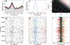Fig. 1 Illustration of the Gibbs sampling procedure applied to the binary MSP J1526-2744. A : photon phases are determined by the current timing model parameters, with probability weights indicated by the grey-scale. B: a short MCMC chain is produced over the template pulse profiles (faint black curves), given these photon phases, and the final step is chosen as the next sample for τ (solid red curve). C: the relative likelihoods as a function of phase for each Gaussian component in the template pulse profile are then used, alongside the photon weights, to determine the probabilities for assigning each photon to a single peak (or to the background). D: these assignments are performed randomly according to these probabilities, with the outcomes illustrated by the colours of photons in the panel corresponding to the relevant peak in the panel above (or the grey-scale for photons assigned to the background). E: a short MCMC chain, starting from the red square and following the blue path to the green triangle, is run targeting the marginal likelihood for the hyperparameters, illustrated by the grey-scale and red contour lines at the 1σ, 2σ, and 3σ levels. Here, a power-law timing noise model is assumed, with hyperparameters consisting of the log-amplitude log10 ATN and spectral index yTN. The final sample in the chain is chosen as the next sample for I. F : a weighted least-squares fit is performed using Gaussian likelihoods for all photons assigned to peaks in the template, constrained by the prior distribution defined by the chosen sample of I. A single sample for the timing model (green curve) is chosen from the posterior distribution that results from this fit (illustrated by the faint black lines). Here, the sinusoidal curve whose amplitude grows with time indicates a significant detection of proper motion. The photon phases in panel A are then updated by these resulting phase shifts, and the process repeats.

3 Demonstrations

In this section, we demonstrate the Gibbs sampling timing method in three representative cases: (1) timing a ‘simple’ binary millisecond pulsar without obvious TN or orbital period variations, showing that it returns posterior distributions that are consistent with those found with existing exact methods that sample the full posterior distribution; (2) simulations of millisecond pulsars with ‘red’ TN processes, which show that our method correctly estimates the amplitudes and spectral indices of these noise processes; and (3) timing of the original black-widow binary pulsar, B1957+20, which exhibits significant orbital period variability, but which is one of the pulsars that contributes most strongly to the GPTA constraints on the GWB.

3.1 PSR J1526-1744: Basic timing model example

We first demonstrate the accuracy of the Gibbs sampling results by running it on a millisecond pulsar that does not require a complicated timing model, and comparing the results to those that were obtained using the existing emcee-based method that samples from the original posterior distribution, p(θ, τ | D). For this demonstration, we used the Fermi-LAT dataset used by Burgay et al. (2024) for the binary MSP J1526−2744.

We here assume improper uniform priors on all timing model parameters, which consist of: right ascension α, declination δ and corresponding proper motions, μ_α cos δ and μ^ spin frequency f and its first derivative f; and orbital parameters A₁, T_asc, P_orb = 1/f_orb and the two Laplace-Lagrangian parameters, η and κ, parameterising eccentricity (Edwards et al. 2006). We do not include any noise components, and therefore have no hyperparameters to fit. We assume a uninformative Dirichlet distribution prior on the two template peak amplitudes, A_k, and un-pulsed component (1 − Σ_kA_k), which ensures these sum to unity. We assume uniform priors on the peak centres, p(μ_k) = I, and a Jeffreys prior for the peak widths, p(σ_k) = 1 /σ_k.

The results are shown in Figure 2. We find that the posterior distributions returned by the two sampling methods are indistinguishable from one another. This shows that the Gibbs sampling approach to marginalising over the latent variables successfully recovers the full posterior distribution.

3.2 Timing noise simulations

To test the robustness of the TN parameter estimates from the Gibbs sampling technique, we simulated and timed 200 pulsars with different levels of TN, and constructed Probability-Probability plots, PP-plots, for the hyperparameters. A PP-plot is a common statistical visualisation tool used to check for possible intrinsic biases in a recovery method for a specific parameter or set of parameters from a set of simulated datasets. The y-axis corresponds to the fractional number of times the injected value lies within the estimated credible interval indicated on the x-axis. When the recovery is unbiased, the PP-plot curve closely follows the diagonal. (See Cook et al. (2006); Talts et al. (2020); Wilk & Gnanadesikan (1968) for more details.)

The simulation method implemented here takes as input the weight distribution, template pulse profile and timing model of a real pulsar and generates new photon arrival times. For the analysis presented here, the simulated pulsars have the same weights, timing model and template of PSR J1939+2134. For each simulation, we first randomise the order of the photon probability weights. For each photon, j, we then generate a uniform random number, u_j between 0 and 1. If u_j > w′_j, where w′_j is the weight of the j-th photon in the randomised weights list, the photon is assigned to the background and its phase is drawn from a uniform distribution between 0 and 1. If u_j < w_j, the photon is assigned to the pulsar and the phase is sampled from the normalised pulse template. We now have a new weight and phase Φ′_j for each photon. We compute the difference in phase between the new phase and the phase Φ_j of the original time of arrival, according to the chosen timing model, and update the time of arrival: t′_i = t_i + (Φ′_i − Φ_i)/f₀, where f₀ is the spin frequency. In this way, we obtained a set of realistic pulsar photon observations, but where the only noise present is due to the random sampling of the phase distribution.

From here, we add additional time delays due to a TN process. Given a function that describes the power spectral density of the signal process as a function of frequency, we build the corresponding time-domain covariance matrix, and use that to define a zero-mean multivariate Gaussian distribution from which we sample a realisation of time delays. To inject the TN in the simulated data, we simply add these time delays to the simulated noise-free photon arrival times.

We simulated 200 pulsars with TN described by a smoothly broken power-law PSD:

$$S(f)=\frac{A^2}{12{\pi }^2}{\left(\frac{f_{\mathrm{c}}}{1{\mathrm{y}\mathrm{r}}^{-1}}\right)}^{-\gamma }{(1+{\left(\frac{f}{f_{\mathrm{c}}}\right)}^2)}^{-\gamma /2}{\mathrm{y}\mathrm{r}}^3,$$(38)

with dimensionless amplitude, A, cutoff frequency, f;, and spectral index, γ. The corresponding time-domain covariance function for this power spectrum is the Matérn function (Rasmussen & Williams 2005).

In our analysis, we simulated 12 years of observations and f_c was set to an arbitrarily low value of 1/(80 yr), such that the noise process is effectively a pure power-law over the frequencies spanned by the data. For each realisation, we sampled the TN amplitude and slope from the uniform priors: log₁₀ A_TN ∊ [−16, -12] and γ_TN ∊ [1,7]. TN was significantly detectable for amplitudes log₁₀(A_TN) ≳ -13 at γ ≈ 4, and at lower amplitudes for steeper spectra.

In Figure 3 we show the results for (i) the recovery of both the TN log-amplitude (solid line) and slope (dashed line) from a set of 200 simulated pulsars, and (ii) the TN log-amplitude recovery from another set of 200 pulsars whose TN slope was fixed to the simulated value of 13/3, which is the expected value for a GWB produced by a population of supermassive black hole binaries (dotted line). The results closely follow the diagonal of the plot and are always within the 3-σ region of the expected distribution for an unbiased recovery. Thus, there is no indication for intrinsic biases in the recovery of those hyperparameters and their uncertainties.

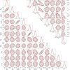Fig. 2 Comparison between the posterior samples obtained via Gibbs sampling (red) and those obtained using the existing emcee method (black), for the binary millisecond pulsar PSR J1526-2744. Template pulse profile parameters are shown in the upper right corner, while timing model parameters are shown in the lower left. There are no strong correlations between pairs of parameters across these two blocks. Contour lines are at the 1σ, 2σ, and 3σ levels.

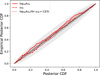Fig. 3 PP-plot for the recovery of the TN amplitude and slope, as defined in Eq. (38), from 200 simulated pulsars. We also show the case of the amplitude recovery from datasets where the slope was fixed to 13/3 (predicted value for a GWB signal). The grey areas are the 1σ and 3σ confidence intervals from the predicted distribution (black diagonal).

3.3 PSR B1957+20: Orbital period variations and timing noise modelling

The previous subsections have demonstrated that the Gibbs sampling method correctly samples the full posterior distribution, and obtains reliable estimates for noise model hyperparameters in addition to the timing model. In this section, we apply this method to one particular pulsar of interest, the original black-widow binary pulsar B1957+20 (also known as PSR J1959+2048). This pulsar is one of the fastest gamma-ray MSPs, and has the narrowest known gamma-ray pulse (in absolute terms) with a full-width at half-maximum of around 25 μs (Guillemot et al. 2012; Ajello et al. 2021). This makes it one of the most important pulsars in the GPTA, with the third lowest upper limit on the GWB in the array.

However, like many spider binaries, this binary also exhibits orbital period variations. In GPTA Paper I, this pulsar was timed using a Taylor series expansion of the orbital frequency. It was found that fixing the orbital frequency derivatives to their nominal values reduced the upper limit on the TN/GWB amplitude by a factor of two, compared to a model where they were free to vary. Furthermore, this was one of only two pulsars, both black widows, for which excess white noise components were favoured in the model. These properties motivate more careful modelling of the OPVs and TN spectrum in this system.

We performed the Gibbs sampling analysis on the dataset used in GPTA Paper I, fitting for both TN and OPVs using Fourier bases with constrained power spectra. We modelled both the OPV and GWB noise processes with broken powerlaw PSDs, as defined in Eq. (38). For the GWB, we fixed the spectral index to the predicted γ_GWB = 13/3. Since the cutoff frequency is expected to be lower than the lowest Fourier frequency for our dataset, we fixed it to the arbitrarily low value of f :,_GWB = 10⁻² yr⁻¹. To obtain an upper limit on the GWB amplitude, we placed a uniform prior on the amplitude (not the log-amplitude, which would lead to the upper limit depending on the lower bound of our prior), with A_GWB < 10⁻¹⁰.

For the OPV spectrum, we used a log-uniform prior on the amplitude −15 < log₁₀ A_OPV < -5. We found in other binaries (Clark et al. 2021; Thongmeearkom et al. 2024) that a pure power-law model for the OPV spectrum does not always provide a good fit, and so we keep f_c,OPV free, with a log-uniform prior between 1/10T_obs < f_c,OPV < 10/T_obs. For the spectral index, we adopted a uniform prior 0 < γ_OPV < 10. The results are illustrated in Figure 4, which shows the posterior distributions of the template pulse profile, the pulse and orbital phase variations and their PSDs, and in Figure 5 which shows the posterior distributions on the GWB and OPV hyperparameters. As in GPTA Paper I, we find no evidence for a GWB-like TN component, with a 95% confidence upper limit of A_GWB < 9.2 × 10⁻¹⁴.

4 Discussion

We have presented a new method for timing gamma-ray pulsars, based on a latent variable approach for tackling the mixture-model likelihood function, and a Gibbs sampling scheme to jointly estimate posterior distributions for the timing model, noise parameters and the template pulse profile. In this section, we discuss possible applications and extensions of this method.

One of the first broad applications of gamma-ray pulsar timing was the investigation of TN in young pulsars by Kerr et al. (2015). This study used a ToA-based approach, which cannot always be applied to faint pulsars. Since then, the known gamma-ray pulsar population has grown, and the duration of Fermi-LAT data has more than doubled. We used this Gibbs sampling method to time two young radio-quiet pulsars in Clark et al. (2025), finding that one had an unusual excess of TN at frequencies around 1 yr⁻¹, which could be due to magnetospheric state switching like that seen in radio pulsars by Lyne et al. (2010) and Lower et al. (2025). A study of young pulsar TN over the longer data span, across the larger gamma-ray pulsar population, and using a more sensitive timing method may yield new insights.

Another timely application is the GPTA’s attempts to constrain the GWB. In GPTA Paper I, two timing approaches were used to place limits on the amplitude of the GWB. The first used the same ToA-based approach as in Kerr et al. (2015), with a cadence of a few months. The second method, which was found to be slightly more sensitive, particularly for fainter pulsars, used the full photon likelihood of Equation (15), making a Gaussian approximation to the posterior distribution on θ that could be integrated to compute the marginal likelihood for 1. This offers equivalent sensitivity to our Gibbs sampling method, and also enables noise parameter fitting, but does not contain a marginalisation over the uncertain template pulse profile. Furthermore, this method did not provide a way to search for correlated noise between pulsars following the predicted Hellings-Downs (HD) curve.

Valtolina & van Haasteren (2025) have since developed a Fourier-domain likelihood for GWB-like inter-pulsar correlations. This method requires samples from the posterior distributions of the TN Fourier coefficients from single-pulsar analyses, with fixed noise hyperparameters, which can be obtained from our Gibbs sampler. Combining these two methods therefore allows us to obtain robust estimates for the parameters of an HD-correlated GWB signal, using an un-binned photon-by-photon approach where uncertainties in the template pulse profile and timing model parameters have been marginalised over. We explored this in Valtolina et al. (2026), where we use the Gibbs sampling scheme and Fourier-domain PTA likelihood of Valtolina & van Haasteren (2025) on the GPTA Paper I dataset, finding a ∼ 20% increase in the upper limit for A_GWB. While the updated constraint is slightly weaker, we found, using simulated gamma-ray PTA datasets produced using the same method applied here in Section 3, that our Gibbs-sampling approach including the template pulse profile marginalisation provided a more robust estimate of the GWB amplitude, compared to the ToA-based approach which tended to underestimate it.

A key motivation for the GPTA is that the gamma-ray data is insensitive to time-varying propagation effects that can bias radio ToA measurements (e.g. DM, scattering and solar-wind variations). Our Gibbs sampling method allows us to incorporate both radio and gamma-ray timing data simultaneously, by simply including the radio ToAs as additional Gaussian terms in Equation (29), and adding appropriate basis vectors accounting for DM and associated noise processes to the design matrix (with radio-frequency dependent derivatives set to zero for all gamma-ray photons). This joint radio and gamma-ray timing capability has already been demonstrated for recently discovered black-widow and redback binaries with a small number of radio ToAs (Burgay et al. 2024; Belmonte Díaz et al. 2025), but the full power of the method would be in jointly fitting radio and gamma-ray PTA data, where correlations between red noise and DM variations would be partially broken by the gamma-ray data.

In Section 3.3, we demonstrated the timing method on PSR B1957+20, a black-widow binary with significant OPVs, which provides one of the most stringent gamma-ray constraints on the GWB. For this search we allowed all timing model parameters to vary in the fit and additionally marginalised over the template pulse profile, rather than assuming a fixed pulse shape. The resulting 95% confidence upper limit of A_GWB < 9.2 × 10⁻¹⁴ is larger than the GPTA Paper I ToA-based upper limit of A_GWB < 8.2 × 10⁻¹⁴, and the GPTA Paper I photon-by-photon upper limits of A_GWB < 6.2 × 10⁻¹⁴, and A_GWB < 2.8 × 10⁻¹⁴ obtained by fixing the astrometry and orbital parameters to their best-fitting values. This may indicate that our marginalisation over template shapes and our Gaussian-process approach to fitting OPVs offer more conservative uncertainties that are less likely to be affected by over-fitting.

This method also allows us to make quantitative statements about the OPV process. The OPVs here have a fractional amplitude of ∆P_orb/P_orb ∼ 10⁻⁷, very similar to that found in earlier radio timing of this pulsar (Arzoumanian et al. 1994). Using the relations in Voisin et al. (2020b), we find that this fractional change in orbital period corresponds to a fractional change in the companion star’s gravitational quadrupole moment of around 2 × 10⁻⁵k⁻¹, where k₂ is the (unknown) apsidal motion constant. For the black-widow PSR J2051−0827, Voisin et al. (2020b) estimated a lower bound of k₂ > 10⁻³. Assuming a similar value for PSR B1957+20 implies fractional quadrupole moment changes of less than a few per cent. These values are very similar to those estimated for redback binaries (Clark et al. 2021; Thongmeearkom et al. 2024), despite the much lighter companion here.

The cutoff frequency, f_c,OPV does not have a well-constrained lower limit, meaning that both pure power-law models (i.e. with f_c,OPV ≪ 1/T_obs), and those with cutoffs around f_c,OPV ≈ 1/(6 yr) are compatible with the data. If we restrict the posterior samples to those describing power-law like models (i.e., samples with f_c,OPV < 1/T_obs) then we find spectral indices of γ ≈ 5 ± 1. We found power-law like processes in other binaries with similar spectral indices (Thongmeearkom et al. 2024; Burgay et al. 2024), close to the value of γ = 4 that would result from a random walk in the orbital period or gravitational quadrupole moment. However, other binaries have OPV spectra with significant cutoffs and/or much steeper spectra (Clark et al. 2021; Thongmeearkom et al. 2024; Belmonte Díaz et al. 2025) suggesting this property is not universal.

Corcoran et al. (2026) and Rosenthal et al. (2025) timed six radio spider binaries in globular clusters, and used a similar Gaussian-process model to measure the OPV spectra for three of these, but found significantly shallower spectra, with γ ≈ 1. We re-fit their orbital phase measurements for all six systems using a Gaussian process with a Matérn covariance function (whose PSD is the smoothly broken power-law model used here), and found that all had γ > 4, suggesting that the Lomb-Scargle method used by Corcoran et al. (2026) and Rosenthal et al. (2025) did not correctly account for spectral leakage from low frequencies (e.g. Coles et al. 2011).

So far, quantitative estimates of OPV processes such as these have mostly been applied to individual pulsars, but the Fermi LAT has now detected gamma-ray pulsations from a population of more than 50 spider binaries (Smith et al. 2023). The Gaussian process model for OPVs, and the Gibbs sampling method presented here, have made timing studies of spiders in the Fermi -LAT data tractable. A consistent treatment of this population may allow for the identification of trends between OPV parameters and other binary properties (e.g. orbital period, companion mass, etc.) that could provide valuable insight into the origin of this behaviour. Furthermore, these methods allow us to include several bright gamma-ray redback systems in the next GPTA data release, increasing its sensitivity and providing further independence from radio PTA efforts, where redbacks are usually excluded due to the detrimental effects of eclipses and their associated DM variations.

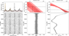Fig. 4 Results of Gibbs-sampling analysis of PSR B1957+20. Left panels show the photon phases (bottom) and integrated pulse profile (top) according to the best-fitting timing model. Faint black curves on the pulse profile plot show individual posterior samples for the template pulse profile, with the best-fitting model shown in orange. Middle panels illustrate the posterior uncertainty on the photon phases (bottom), and on the PSD of the GWB-like timing noise component that we searched for (top). The dashed black line shows the estimated white-noise level, while the red shaded regions show the 1σ and 2σ constraints on a putative power-law noise component with spectral index γ = 13/3. Black lines show the posterior uncertainties on the individual Fourier powers; no significant power is detected above the white noise level at any frequency, and so these posteriors all closely follow the priors. Right panels show the same, but for orbital phase noise, in which a steep spectrum process is detected.

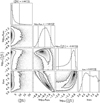Fig. 5 Posterior distribution for the GWB and OPV hyperparameters for PSR B1957+20. Contours on the 2D distributions are at the 1σ and 2σ levels, while dashed vertical lines on the 1D marginal distributions indicate the 5%, 50%, and 95% quantiles.

5 Conclusions

We have presented a new method for timing gamma-ray pulsars in the Fermi-LAT data. This method is based on transforming the fitting problem into a Gaussian process analysis through the introduction of latent variables that associate each photon to a single component of a model pulse profile, and using the technique of Gibbs sampling to marginalise over these latent variables. This technique enables us to efficiently fit complicated timing models and estimate parameters that describe red TN and stochastic OPVs, all the while accounting for uncertainties arising from the unknown intrinsic pulse profile shape.

We implemented this Gibbs sampling procedure in a python package called shoogle, which is based on the PINT pulsar timing package. We demonstrated that shoogle provides posterior distributions that are consistent with those obtained using previous methods. We also simulated 200 new realisations of the gamma-ray MSP J1939+2134 with additional TN, and found that our method provides unbiased estimates for TN parameters with robust uncertainties.

Finally, we demonstrated the new timing method on a 12-year dataset for the original black-widow binary PSR B1957+20, where we were able to obtain an upper limit on a red-spectrum GWB-like noise process of A_GWB < 9.2 × 10⁻¹⁴, somewhat larger than that obtained in GPTA Paper I, while simultaneously modelling the orbital period variations as a Gaussian process. We found that the properties of these variations are very similar to those observed in other redback and black-widow binaries.

Our new method was used alongside the work in Valtolina & van Haasteren (2025) to re-analyse the GPTA Paper I dataset and to perform a search for correlated noise produced by a stochastic gravitational wave background without having to bin the LAT data into six-month segments. This resulted in a slightly higher, but hopefully more robust, upper limit of A_GWB < 1.2 × 10⁻¹⁴ (Valtolina et al. (2026). These methods will be used to analyse the next GPTA data release, alongside additional improvements such as incorporating photon-energy-dependent pulse profile models to boost sensitivity. Furthermore, our method provides a simple route for future joint modelling of radio and gammaray pulsar observations, which may significantly improve radio PTA sensitivity by partially breaking correlations between DM variations and the GWB-induced residuals.

Acknowledgements

We are very grateful to Matthew Kerr for insightful discussions on gamma-ray pulsar timing methods, and for helpful comments on the manuscript. We also thank Xian Hou for reviewing the paper on behalf of the Fermi LAT Collaboration, and Kyle Corcoran for helpful discussion regarding their timing of globular cluster redbacks. SV acknowledges financial support from the European Research Council (ERC) starting grant ‘GIGA’ (grant agreement number: 101116134). The Fermi LAT Collaboration acknowledges generous ongoing support from a number of agencies and institutes that have supported both the development and the operation of the LAT as well as scientific data analysis. These include the National Aeronautics and Space Administration and the Department of Energy in the United States, the Commissariat à l’Energie Atomique and the Centre National de la Recherche Scientifique/Institut National de Physique Nucléaire et de Physique des Particules in France, the Agenzia Spaziale Italiana and the Istituto Nazionale di Fisica Nucleare in Italy, the Ministry of Education, Culture, Sports, Science and Technology (MEXT), High Energy Accelerator Research Organization (KEK) and Japan Aerospace Exploration Agency (JAXA) in Japan, and the K. A. Wallenberg Foundation, the Swedish Research Council and the Swedish National Space Board in Sweden. Additional support for science analysis during the operations phase is gratefully acknowledged from the Istituto Nazionale di Astrofisica in Italy and the Centre National d’Études Spatiales in France. This work performed in part under DOE Contract DE-AC02-76SF00515.

References

Appendix A Glossary

All Tables

All Figures

Fig. 1 Illustration of the Gibbs sampling procedure applied to the binary MSP J1526-2744. A : photon phases are determined by the current timing model parameters, with probability weights indicated by the grey-scale. B: a short MCMC chain is produced over the template pulse profiles (faint black curves), given these photon phases, and the final step is chosen as the next sample for τ (solid red curve). C: the relative likelihoods as a function of phase for each Gaussian component in the template pulse profile are then used, alongside the photon weights, to determine the probabilities for assigning each photon to a single peak (or to the background). D: these assignments are performed randomly according to these probabilities, with the outcomes illustrated by the colours of photons in the panel corresponding to the relevant peak in the panel above (or the grey-scale for photons assigned to the background). E: a short MCMC chain, starting from the red square and following the blue path to the green triangle, is run targeting the marginal likelihood for the hyperparameters, illustrated by the grey-scale and red contour lines at the 1σ, 2σ, and 3σ levels. Here, a power-law timing noise model is assumed, with hyperparameters consisting of the log-amplitude log10 ATN and spectral index yTN. The final sample in the chain is chosen as the next sample for I. F : a weighted least-squares fit is performed using Gaussian likelihoods for all photons assigned to peaks in the template, constrained by the prior distribution defined by the chosen sample of I. A single sample for the timing model (green curve) is chosen from the posterior distribution that results from this fit (illustrated by the faint black lines). Here, the sinusoidal curve whose amplitude grows with time indicates a significant detection of proper motion. The photon phases in panel A are then updated by these resulting phase shifts, and the process repeats.

In the text

Fig. 2 Comparison between the posterior samples obtained via Gibbs sampling (red) and those obtained using the existing emcee method (black), for the binary millisecond pulsar PSR J1526-2744. Template pulse profile parameters are shown in the upper right corner, while timing model parameters are shown in the lower left. There are no strong correlations between pairs of parameters across these two blocks. Contour lines are at the 1σ, 2σ, and 3σ levels.

In the text

	Fig. 3 PP-plot for the recovery of the TN amplitude and slope, as defined in Eq. (38), from 200 simulated pulsars. We also show the case of the amplitude recovery from datasets where the slope was fixed to 13/3 (predicted value for a GWB signal). The grey areas are the 1σ and 3σ confidence intervals from the predicted distribution (black diagonal).
In the text

Fig. 4 Results of Gibbs-sampling analysis of PSR B1957+20. Left panels show the photon phases (bottom) and integrated pulse profile (top) according to the best-fitting timing model. Faint black curves on the pulse profile plot show individual posterior samples for the template pulse profile, with the best-fitting model shown in orange. Middle panels illustrate the posterior uncertainty on the photon phases (bottom), and on the PSD of the GWB-like timing noise component that we searched for (top). The dashed black line shows the estimated white-noise level, while the red shaded regions show the 1σ and 2σ constraints on a putative power-law noise component with spectral index γ = 13/3. Black lines show the posterior uncertainties on the individual Fourier powers; no significant power is detected above the white noise level at any frequency, and so these posteriors all closely follow the priors. Right panels show the same, but for orbital phase noise, in which a steep spectrum process is detected.

In the text

	Fig. 5 Posterior distribution for the GWB and OPV hyperparameters for PSR B1957+20. Contours on the 2D distributions are at the 1σ and 2σ levels, while dashed vertical lines on the 1D marginal distributions indicate the 5%, 50%, and 95% quantiles.
In the text

References

- Abdo, A. A., Ackermann, M., Ajello, M., et al. 2009, Science, 325, 840 [Google Scholar]
- Abdo, A. A., Ajello, M., Allafort, A., et al. 2013, ApJS, 208, 17 [Google Scholar]
- Ajello, M., Atwood, W. B., Axelsson, M., et al. 2021, ApJS, 256, 12 [NASA ADS] [CrossRef] [Google Scholar]
- Allafort, A., Baldini, L., Ballet, J., et al. 2013, ApJ, 777, L2 [NASA ADS] [CrossRef] [Google Scholar]
- Allen, B., & Romano, J. D. 2025, Phys. Rev. Lett., 134, 031401 [Google Scholar]
- Applegate, J. H. 1992, ApJ, 385, 621 [Google Scholar]
- Applegate, J. H., & Patterson, J. 1987, ApJ, 322, L99 [NASA ADS] [CrossRef] [Google Scholar]
- Arzoumanian, Z., Fruchter, A. S., & Taylor, J. H. 1994, ApJ, 426, L85 [NASA ADS] [CrossRef] [Google Scholar]
- Atwood, W. B., Abdo, A. A., Ackermann, M., et al. 2009, ApJ, 697, 1071 [CrossRef] [Google Scholar]
- Balakrishnan, V., Freire, P. C. C., Ransom, S. M., et al. 2023, ApJ, 942, L35 [CrossRef] [Google Scholar]
- Belmonte Díaz, S., Thongmeearkom, T., Phosrisom, A., et al. 2025, MNRAS, 543, 3019 [Google Scholar]
- Bickel, P., Kleijn, B., & Rice, J. 2008, ApJ, 685, 384 [NASA ADS] [CrossRef] [Google Scholar]
- Bochenek, C., Ransom, S., & Demorest, P. 2015, ApJ, 813, L4 [NASA ADS] [Google Scholar]
- Bradbury, J., Frostig, R., Hawkins, P., et al. 2018, JAX: composable transformations of Python+NumPy programs [Google Scholar]
- Burgay, M., Nieder, L., Clark, C. J., et al. 2024, A&A, 691, A315 [NASA ADS] [CrossRef] [EDP Sciences] [Google Scholar]
- Cabezas, A., Corenflos, A., Lao, J., et al. 2024, arXiv e-prints [arXiv:2402.10797] [Google Scholar]
- Clark, C. J., Pletsch, H. J., Wu, J., et al. 2015, ApJ, 809, L2 [NASA ADS] [CrossRef] [Google Scholar]
- Clark, C. J., Nieder, L., Voisin, G., et al. 2021, MNRAS, 502, 915 [NASA ADS] [CrossRef] [Google Scholar]
- Clark, C. J., Di Mauro, M., Wu, J., et al. 2025, ApJ, 994, 149 [Google Scholar]
- Coles, W., Hobbs, G., Champion, D. J., Manchester, R. N., & Verbiest, J. P. W. 2011, MNRAS, 418, 561 [Google Scholar]
- Cook, S. R., Gelman, A., & Rubin, D. B. 2006, J. Computat. Graph. Statist., 15, 675 [Google Scholar]
- Corcoran, K. A., Ransom, S. M., Rosenthal, A. C., et al. 2026, ApJ, 998, 161 [Google Scholar]
- Crisostomi, M., van Haasteren, R., Meyers, P. M., & Vallisneri, M. 2025, arXiv e-prints [arXiv:2506.13866] [Google Scholar]
- Csató, L., & Opper, M. 2002, Neural Computat., 14, 641 [Google Scholar]
- Daemi, A., Kodamana, H., & Huang, B. 2019, J. Process Control, 81, 209 [Google Scholar]
- Deneva, J. S., Ray, P. S., Camilo, F., et al. 2016, ApJ, 823, 105 [Google Scholar]
- Edwards, R. T., Hobbs, G. B., & Manchester, R. N. 2006, MNRAS, 372, 1549 [Google Scholar]
- Ellis, J. A., Vallisneri, M., Taylor, S. R., & Baker, P. T. 2020, https://doi.org/10.5281/zenodo.4059815 [Google Scholar]
- Fiori, A., Razzano, M., Harding, A. K., et al. 2024, A&A, 685, A70 [NASA ADS] [CrossRef] [EDP Sciences] [Google Scholar]
- Foreman-Mackey, D., Hogg, D. W., Lang, D., & Goodman, J. 2013, PASP, 125, 306 [Google Scholar]
- Geman, S., & Geman, D. 1984, IEEE Trans. Pattern Anal. Mach. Intell., PAMI-6, 721 [Google Scholar]
- Guillemot, L., Johnson, T. J., Venter, C., et al. 2012, ApJ, 744, 33 [NASA ADS] [CrossRef] [Google Scholar]
- Gundersen, A., & Cornish, N. J. 2025, arXiv e-prints [arXiv:2510.12917] [Google Scholar]
- Hoffman, M. D., & Gelman, A. 2011, arXiv e-prints [arXiv:1111.4246] [Google Scholar]
- Iraci, F., Chalumeau, A., Tiburzi, C., et al. 2024, A&A, 692, A170 [NASA ADS] [CrossRef] [EDP Sciences] [Google Scholar]
- Kerr, M. 2011, ApJ, 732, 38 [NASA ADS] [CrossRef] [Google Scholar]
- Kerr, M., Ray, P. S., Johnston, S., Shannon, R. M., & Camilo, F. 2015, ApJ, 814, 128 [NASA ADS] [CrossRef] [Google Scholar]
- Larsen, B., Mingarelli, C. M. F., Hazboun, J. S., et al. 2024, ApJ, 972, 49 [Google Scholar]
- Lentati, L., Alexander, P., Hobson, M. P., et al. 2013, Phys. Rev. D, 87, 104021 [NASA ADS] [CrossRef] [Google Scholar]
- Lentati, L., Alexander, P., Hobson, M. P., et al. 2014, MNRAS, 437, 3004 [NASA ADS] [CrossRef] [Google Scholar]
- Lower, M. E., Karastergiou, A., Johnston, S., et al. 2025, MNRAS, 538, 3104 [Google Scholar]
- Luo, J., Ransom, S., Demorest, P., et al. 2021, ApJ, 911, 45 [NASA ADS] [CrossRef] [Google Scholar]
- Lyne, A., Hobbs, G., Kramer, M., Stairs, I., & Stappers, B. 2010, Science, 329, 408 [NASA ADS] [CrossRef] [Google Scholar]
- Neal, R. M. 2000, arXiv e-prints [arXiv:physics/0009028] [Google Scholar]
- Ng, C., Bailes, M., Bates, S. D., et al. 2014, MNRAS, 439, 1865 [NASA ADS] [CrossRef] [Google Scholar]
- Nieder, L., Clark, C. J., Bassa, C. G., et al. 2019, ApJ, 883, 42 [NASA ADS] [CrossRef] [Google Scholar]
- Nieder, L., Clark, C. J., Kandel, D., et al. 2020, ApJ, 902, L46 [NASA ADS] [CrossRef] [Google Scholar]
- Nieder, L., Kerr, M., Clark, C. J., et al. 2022, ApJ, 931, L3 [NASA ADS] [CrossRef] [Google Scholar]
- Padmanabh, P. V., Ransom, S. M., Freire, P. C. C., et al. 2024, A&A, 686, A166 [NASA ADS] [CrossRef] [EDP Sciences] [Google Scholar]
- Panin, A. G., & Sokolova, E. V. 2025, A&A, 697, A178 [NASA ADS] [CrossRef] [EDP Sciences] [Google Scholar]
- Pletsch, H. J., & Clark, C. J. 2015, ApJ, 807, 18 [Google Scholar]
- Pletsch, H. J., Guillemot, L., Allen, B., et al. 2012a, ApJ, 755, L20 [Google Scholar]
- Pletsch, H. J., Guillemot, L., Allen, B., et al. 2012b, ApJ, 744, 105 [Google Scholar]
- Rasmussen, C. E., & Williams, C. K. I. 2005, Gaussian Processes for Machine Learning (Adaptive Computation and Machine Learning) (The MIT Press) [Google Scholar]
- Ray, P. S., Kerr, M., Parent, D., et al. 2011, ApJS, 194, 17 [NASA ADS] [CrossRef] [Google Scholar]
- Ray, P. S., Ransom, S. M., Cheung, C. C., et al. 2013, ApJ, 763, L13 [NASA ADS] [CrossRef] [Google Scholar]
- Ray, P. S., Polisensky, E., Parkinson, P. S., et al. 2020, RNAAS, 4, 37 [Google Scholar]
- Ridolfi, A., Freire, P. C. C., Torne, P., et al. 2016, MNRAS, 462, 2918 [Google Scholar]
- Roberts, M. S. E. 2013, in IAU Symposium, 291, Neutron Stars and Pulsars: Challenges and Opportunities after 80 years, ed. J. van Leeuwen, 127 [Google Scholar]
- Rosenthal, A. C., Ransom, S. M., Corcoran, K. A., et al. 2025, ApJ, 982, 170 [Google Scholar]
- Seiferth, D., Chowdhary, G., Mühlegg, M., & Holzapfel, F. 2017, in 2017 American Control Conference (ACC), 3134 [Google Scholar]
- Shaifullah, G., Verbiest, J. P. W., Freire, P. C. C., et al. 2016, MNRAS, 462, 1029 [Google Scholar]
- Smith, D. A., Abdollahi, S., Ajello, M., et al. 2023, ApJ, 958, 191 [NASA ADS] [CrossRef] [Google Scholar]
- Susarla, S. C., Chalumeau, A., Tiburzi, C., et al. 2024, A&A, 692, A18 [NASA ADS] [CrossRef] [EDP Sciences] [Google Scholar]
- Susobhanan, A. 2025, ApJ, 980, 165 [Google Scholar]
- Susobhanan, A., Kaplan, D. L., Archibald, A. M., et al. 2024, ApJ, 971, 150 [Google Scholar]
- Takata, J., Wang, H. H., Lin, L. C. C., et al. 2020, ApJ, 890, 16 [NASA ADS] [CrossRef] [Google Scholar]
- Talts, S., Betancourt, M., Simpson, D., Vehtari, A., & Gelman, A. 2020, arXiv e-prints [arXiv:1804.06788] [Google Scholar]
- The Fermi-LAT Collaboration (Ajello, M., et al.) 2022, Science, 376, 521 [NASA ADS] [CrossRef] [Google Scholar]
- Thongmeearkom, T., Clark, C. J., Breton, R. P., et al. 2024, MNRAS, 530, 4676 [CrossRef] [Google Scholar]
- Valtolina, S., & van Haasteren, R. 2025, Phys. Rev. D, 112, 043046 [Google Scholar]
- Valtolina, S., Clark, C. J., van Haasteren, R., et al. 2026, Phys. Rev. D, 113, 063061 [Google Scholar]
- van Haasteren, R., & Vallisneri, M. 2014, Phys. Rev. D, 90, 104012 [NASA ADS] [CrossRef] [Google Scholar]
- van Haasteren, R., & Vallisneri, M. 2015, MNRAS, 446, 1170 [NASA ADS] [CrossRef] [Google Scholar]
- van Haasteren, R., Levin, Y., McDonald, P., & Lu, T. 2009, MNRAS, 395, 1005 [NASA ADS] [CrossRef] [Google Scholar]
- Voisin, G., Breton, R. P., & Summers, C. 2020a, MNRAS, 492, 1550 [Google Scholar]
- Voisin, G., Clark, C. J., Breton, R. P., et al. 2020b, MNRAS, 494, 4448 [Google Scholar]
- Wilk, M. B., & Gnanadesikan, R. 1968, Biometrika, 55, 1 [Google Scholar]