| Issue |
A&A
Volume 709, May 2026
|
|
|---|---|---|
| Article Number | A182 | |
| Number of page(s) | 15 | |
| Section | Astrophysical processes | |
| DOI | https://doi.org/10.1051/0004-6361/202558692 | |
| Published online | 13 May 2026 | |
A simple relation: Neutron star magnetic field strength and spectral shape at low mass accretion rates
1
Dr. Karl-Remeis-Observatory and Erlangen Centre for Astroparticle Physics, Friedrich-Alexander-Universität Erlangen-Nürnberg, Sternwartstr. 7, 96049 Bamberg, Germany
2
CRESST and Center for Space Sciences and Technology, University of Maryland, Baltimore County, 1000 Hilltop Circle, Baltimore, MD 21250, USA
3
NASA Goddard Space Flight Center, Astrophysics Science Division, Greenbelt, MD 20771, USA
4
University of Maryland, Department of Astronomy, College Park, MD 20742, USA
5
INAF-Osservatorio Astronomico di Roma, Via Frascati 33, 00078 Monte Porzio Catone (RM), Italy
★ Corresponding author: This email address is being protected from spambots. You need JavaScript enabled to view it.
Received:
19
December
2025
Accepted:
23
March
2026
Abstract
Context. The X-ray spectra of neutron stars with moderate magnetic fields (B ∼ 1012 G) in high-mass X-ray binaries (HMXBs) at low X-ray luminosities (LX ≲ 1035 erg s−1) are characterized by a double humped shape. This shape has been explained either as the radiation from a two-temperature magnetized atmosphere, where thermal radiation dominates at soft X-rays below about 10 keV, and cyclotron radiation with an imprinted cyclotron line dominates at high energies, or by the complex redistribution of primary X-rays in a structured atmosphere.
Aims. The theoretical explanations of the double humped structure predict the spectra to depend on the magnetic field. We aim to connect the model predictions with observations.
Methods. We analyzed archival NuSTAR observations of four HMXBs consisting of a neutron star and a Be star (BeXRBs), with known magnetic fields at luminosities low enough to show the characteristic double-hump spectrum. We modeled these spectra empirically and derived a relation between the energy of the intersection of the two humps and the magnetic field strength. In a second step, we tested whether this correlation is supported by fitting synthetic spectra simulated with the physically self-consistent polcap model.
Results. We find a linear correlation between the magnetic field strength and the intersection energy for the real BeXRB NuSTAR spectra and polcap-based simulated NuSTAR spectra alike.
Conclusions. The effect of the magnetic field on spectral formation results in an observable correlation between the field strength and spectral shape. This derived positive correlation between intersection energy and magnetic field strength also allowed us to roughly estimate the magnetic field strength via our proposed 2-B-12 rule. Additional observations of XRBs and dedicated modeling efforts will be necessary to determine whether this approach is valid beyond the B-field range of a few 1012–1013 G that was tested in this work.
Key words: stars: magnetic field / stars: neutron / pulsars: general / X-rays: binaries
Deceased 17 June 2025.
© The Authors 2026
 Open Access article, published by EDP Sciences, under the terms of the Creative Commons Attribution License (https://creativecommons.org/licenses/by/4.0), which permits unrestricted use, distribution, and reproduction in any medium, provided the original work is properly cited.
This article is published in open access under the Subscribe to Open model. This email address is being protected from spambots. You need JavaScript enabled to view it. to support open access publication.
1. Introduction
Magnetic fields play an important role in our understanding of the environment of magnetized neutron stars (NSs; see, e.g., Harding & Lai 2006). Neutron stars are typically found in binary systems with either a low-mass companion (low-mass X-ray binaries or LMXBs; see, e.g., Mitsuda et al. 1984) or a high-mass companion (high-mass X-ray binaries or HMXBs; see, e.g., Chaty 2011). In the latter case, the companion is typically a supergiant or Be-type massive star. In HMXBs, mass accretion from the stellar companion onto the NS (see, e.g., Ghosh & Lamb 1979) can occur via accretion disks around the NS or via strong stellar winds from the companion. The strong gravitational field of the neutron star governs the dynamics of the accreted matter at large distances. At intermediate distances, however, the neutron star’s strong magnetic field (or B-field) of 1012–1013 G affects the dynamics of the accreted material (see, e.g., Lamb et al. 1973). It modifies the radiative processes involved in reprocessing of radiation close to the neutron star surface and has a crucial effect on spectral formation (Basko & Sunyaev 1975; Araya & Harding 1999).
Magnetic fields of strongly magnetized accreting neutron stars can often be measured directly via cyclotron resonant scattering features (CRSFs), or “cyclotron lines”, in their X-ray spectra (see Staubert et al. 2019, for a review). Cyclotron resonant scattering features are formed due to the quantization of electron momenta perpendicular to the magnetic field axis. Compton scattering in optically thick media and the redistribution of photons with energies close to the energy difference between two adjacent Landau levels result in apparent absorption features with centroid energies close to this energy difference. Cyclotron lines therefore probe the magnetic field strength within the line-forming region, which is typically assumed to be close to the neutron star surface. The observed centroid energy of the CRSF, ECRSF, and the B-field strength are related via the 12-B-12 rule,
 (1)
(1)
where n corresponds to the nth harmonic feature (i.e., n = 1 corresponds to the fundamental line), z is the gravitational redshift due to the NS gravitational field (z = 0.24 for MNS = 1.4 M⊙ and RNS = 12 km), and B is the magnetic field strength in the line-forming region.
Cyclotron resonant scattering features, however, are not the only spectral signatures that can arise from electron quantization. At low mass accretion rates, ≲1016 g s−1, when the pressure of the emitted radiation is insufficient to affect the deceleration of the accretion flow (see, e.g., Basko & Sunyaev 1976; Becker et al. 2012; Mushtukov et al. 2015, for a discussion of the transition to the radiation-dominated regime), it is mainly decelerated by Coulomb collisions (see Meszaros et al. 1983; Harding et al. 1984; Miller et al. 1987, and references therein). The kinematics of the braking process in a strong magnetic field differs significantly from the non-magnetized case. Coulomb collisions can result in multiple excitations of the ambient electrons (Miller et al. 1987, 1989; Nelson et al. 1993), followed by radiative decay and the production of cyclotron photons. This nonthermal (bulk) cyclotron emission, reprocessed in the atmosphere, is thought to produce a noticeable excess in the X-ray spectra (e.g., Nelson et al. 1995; Mushtukov et al. 2021). The (Coulomb-heated) atmospheres consist of two distinct temperature zones, with significantly higher temperatures at the top than deep within the atmosphere and an outward decreasing electron density (see, e.g., Zel’dovich & Shakura 1969; Meszaros et al. 1983; Miller et al. 1989). These effects are thought to be responsible for the formation of the two-component spectra observed in Be X-ray binaries (BeXRBs) at typical luminosities of 1033–1034 erg s−1 (see, e.g., Tsygankov et al. 2019a,b; Lutovinov et al. 2021, and Fig. 1). Mushtukov et al. (2021) showed that the X-ray spectra of a two-temperature magnetized atmosphere – with distinct cold and hot regions and cyclotron emission – exhibit a characteristic double-hump shape: thermal emission dominates at soft X-rays, while reprocessed cyclotron emission, imprinted with a CRSF, appears at higher energies. In their model, nearly all the accretion energy is assumed to be converted into cyclotron emission. However, detailed kinematic calculations indicate that for magnetic fields of ∼5 × 10¹² G, the amount of electron excitations per falling proton can remain relatively low (Miller et al. 1989), potentially reducing the nonthermal cyclotron contribution. Sokolova-Lapa et al. (2021) explored an alternative scenario in which excitation plays only a minor role in spectral formation. In this case, the structure of the atmosphere is affected by strong temperature and density gradients, polarization effects, and complex redistribution during the scattering process in the vicinity of the cyclotron resonance, which still results in a two-component X-ray spectrum with distinct low- and high-energy humps. Both models, that of Mushtukov et al. (2021) and that of Sokolova-Lapa et al. (2021), have been successfully applied to describe the quiescent spectra of BeXRBs. In both models, the formation of the high-energy component is closely related to cyclotron interactions.
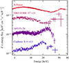 |
Fig. 1. NuSTAR X-ray spectra of BeXRBs in quiescence. The spectra are ordered by decreasing energy at which the hard X-ray-component peaks, from top to bottom. The respective rescaling factors, where required, are given next to the source names. |
In this paper we perform a systematic study of the X-ray spectra of BeXRBs at low luminosity. In Sect. 2, we model X-ray spectra of a selection of BeXRBs with an empirical model consisting of two spectral humps and show that the location of these humps depends on the surface magnetic field of the neutron stars. In Sect. 3, we then use theoretical spectral models for BeXRBs at low mass accretion rates to show that they can in principle reproduce the observed magnetic field dependency. In Sect. 4, we put our results in a physical context and discuss predictions by theoretical models.
2. X-ray spectral analysis of BeXRBs in quiescence
In this section we present our spectral analysis of nine BeXRBs. We describe our source selection in Sect. 2.1 In Sect. 2.2, we introduce semi-physical and phenomenological models that are typically utilized to describe the X-ray spectra of BeXRBs and present the empirical model utilized in this work. In Sect. 2.3 we present our spectral analysis of nine BeXRB NuSTAR spectra and use our results to investigate a potential relation between the hard spectral component and the magnetic field strength in Sect. 2.4.
2.1. Source selection
We carried out a literature study and archive search for all BeXRBs to determine whether the sources are known to enter a state of stable quiescent accretion and, if so, whether archival broadband NuSTAR observations are available. For many systems such as 2RXP J130159.6−635806, GRO J2058+42, IGR J18027-2016, RX J0440.9+4431, and SAX J2103.5+4545, we find that the systems have been observed by NuSTAR only at luminosities exceeding 1035 erg s−1 (Krivonos et al. 2015; Salganik et al. 2025; Lutovinov et al. 2017; Salganik et al. 2023; Brumback et al. 2018), and they are therefore not considered further in this work. The NuSTAR observations of MAXI J1409−619 and MXB 0656-072 indicate that the systems could exhibit X-ray emission caused by stable low-level accretion; the NuSTAR data are, however, insufficient to conduct a broadband spectral analysis with a focus on the intermediate and hard X-ray band (Ghimiray et al. 2024; Raman et al. 2023); they were therefore discarded from the sample.
In summary, we found nine BeXRBs (2SXPS J075542.5−293353 1 (Doroshenko et al. 2021), A0535+26 (Ballhausen et al. 2017; Tsygankov et al. 2019a), Cep X-4 (Vybornov et al. 2017; Sokolova-Lapa et al. 2023b), GRO J1008−57 (Lutovinov et al. 2021; Chen et al. 2021), GX 304−1 (Rouco Escorial et al. 2018; Tsygankov et al. 2019b; Sokolova-Lapa et al. 2021), IGR J21347+4737 (Gorban et al. 2022a; Ghising et al. 2023), MAXI J0655−013 (Pike et al. 2023; Rai et al. 2023), SRGA J124404.1−632232 (Doroshenko et al. 2022), and X Per (Mushtukov et al. 2023; Rodi et al. 2024; Rai et al. 2025), with NuSTAR observations at low luminosities of 1033–1034 erg s−1 that indicate stable quiescent accretion. We based our subsequent spectral analysis on the NuSTAR observations of these nine BeXRBs.
2.2. Semi-physical and phenomenological spectral models
The double humped X-ray spectra of BeXRBs at luminosities of ∼1034 erg s−1 are often described as the sum of two semi-physical models for thermal Comptonization spectra such as comptt (Titarchuk 1994). Examples of the application of such models are observations of GRO J1008−57 (Lutovinov et al. 2021), A0535+26 (Tsygankov et al. 2019a), X Per (Rai et al. 2025), and MAXI J0655−013 (Malacaria et al. 2026). While describing the spectrum of the low-energy component (LEC) with Comptonization is physically motivated, this is less clear for the case of the high-energy component (HEC), which is observed in an energy band where other effects than thermal Comptonization are expected to be at work.
Here, we model the X-ray spectra of BeXRBs in quiescence with a purely empirical model that focuses on measuring the position of the HEC without any physical interpretation. Our primary aim is to describe the spectral positions of the two humps. Since we only want to constrain the continuum shape, we only considered the X-ray spectrum up to the red wing of the HEC and disregard the fundamental CRSF and its blue wing. We modeled the LEC and the red wing of the HEC each with a power law with an exponential cut off (cutoffpl in XSPEC and ISIS). We expected our data above ∼30 keV to be poorly constrained for two reasons. First, the NuSTAR effective area significantly decreases toward high energies (see, e.g., Harrison et al. 2013, Fig. 2). Second, previous observations and their analyses as well as theoretical spectral models predict that the HEC is imprinted with a deep, wide cyclotron line (see, e.g., Tsygankov et al. 2019a; Sokolova-Lapa et al. 2021). While the line itself cannot be resolved in quiescent NuSTAR observations if ECRSF ≳ 45 keV, the absorption and spectral redistribution caused by the cyclotron interaction result in a flux decrease toward higher energies. As a result, typical NuSTAR spectra with exposure times of tens of kiloseconds do not allow us to constrain the HEC reliably, which potentially results in model degeneracies between the photon index Γ2 and the folding energy Efold, which determines the exponential rollover. We therefore decided to fix the photon index of the HEC-modeling power law component Γ2.
While models with Γ2 > 0 generally obtain favorable fit statistics, the spectral models lack physical interpretability due to the fact that in this case, the two cutoffpl components no longer model the two humps, respectively. Additionally, models where Γ2 > 0 imply the unphysical scenario that the two components overlap significantly and that the HEC contributes a few percent of the flux in the soft band. This is not expected based on our theoretical understanding of the spectral formation within inhomogeneous neutron star atmospheres (see, e.g., Sokolova-Lapa et al. 2021, Fig. 4)
A preliminary analysis of X Per showed that fixing Γ2 = −2 is a balance between obtaining a statistically satisfactory description of the data and obtaining a description where each cutoffpl component models one spectral hump, respectively. A more detailed justification is given in Sect. 4.3. From a physical point of view, the HEC-modeling component represents a Wien-like continuum in this case (see, e.g., Nagel 1981; Orlandini & Fiume 2001). In summary, the continuum model can be expressed as
![Mathematical equation: $$ \begin{aligned} F_\mathrm{ph} (E) = \underbrace{K_1 \cdot E^{-\Gamma _1} \cdot \exp \left[-\frac{E}{E_\mathrm{fold,1} }\right]}_\text{LEC}+\underbrace{K_2\cdot E^2 \cdot \exp \left[-\frac{E}{E_\mathrm{fold,2} }\right]}_\text{Wien-like} \text{ red} \text{ wing} \text{ of} \text{ the} \text{ HEC}, \end{aligned} $$](/articles/aa/full_html/2026/05/aa58692-25/aa58692-25-eq2.gif) (2)
(2)
where K1, 2 are the normalizations of the two components, Γ1 and Efold, 1 are the photon index and the folding energy of the LEC, and Efold, 2 is the characteristic energy of the Wien-like component which determines the position and slope of its exponential cut off.
In order to characterize the relative positions of the two spectral components we reparametrize Eq. (2) by introducing their intersection energy, Eint, defined as the energy at which the flux of the two cutoffpl components is equal, which replaces K2 as a model parameter. K2 is therefore given by
![Mathematical equation: $$ \begin{aligned} K_2=K_1 \times E_\mathrm{int} ^{-(\Gamma _1+2)} \times \exp \left[E_\mathrm{int} \times \left(\frac{1}{E_\mathrm{fold,2} }-\frac{1}{E_\mathrm{fold,1} }\right)\right]. \end{aligned} $$](/articles/aa/full_html/2026/05/aa58692-25/aa58692-25-eq3.gif) (3)
(3)
2.3. Spectral analysis utilizing the doublehump model
We based our spectral analysis on archival observations of nine BeXRBs at low luminosities observed with NuSTAR (Harrison et al. 2013). This mission offers the broad band X-ray coverage needed and provides a sufficiently large number of archival observations. See Table B.1 for the parameters of these observations. Where available, we also utilize contemporaneous observations or observations at a similar luminosity level with Swift/XRT (Gehrels et al. 2004; Burrows et al. 2005), XMM-Newton (Jansen et al. 2001; den Herder et al. 2001; Strüder et al. 2001; Turner et al. 2001), NICER (Gendreau et al. 2012, 2016), and Chandra (Weisskopf et al. 2000).
As the doublehump model does not account for absorption features due to cyclotron resonant scattering, it naturally cannot reproduce CRSFs. Therefore, the X-ray spectra of sources exhibiting such features are only modeled up to energies below the CRSF, that is, to 40 keV for A0535+26, 50 keV for GX 304−1, and 25 keV for Cep X-4 2. We utilized the absorption model TBabs (Wilms et al. 2000) with cross sections and abundances as given by Verner et al. (1996) and Wilms et al. (2000), respectively. A preliminary study showed that the absorption column density, NH, can be constrained for all BeXRBs considered, with the exception of Cep X-4, for which we assumed the Galactic H I column density in the direction of the source (HI4PI Collaboration 2016). Including a cross-calibration constant for each detector, fixed to unity for NuSTAR/FPMA, the model applied to each dataset is
 (4)
(4)
Our spectral fits and their residuals are shown in Fig. 2, the fit parameters are given in the lower half of Table B.1.
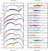 |
Fig. 2. Spectral fit of the doublehump model to quiescent X-ray spectra of nine BeXRBs. Left panel: Unfolded E × FE spectra and fit model (solid line); the dashed lines indicate the two components of the doublehump model. The spectra are separated vertically for improved perceptibility, ordered by descending intersection energy from top to bottom, and to this end have been rescaled by the factors given on the left y-axis of the left panel. The spectra have also been rescaled to match NuSTAR/FPMA according to the cross-calibration constants. Right panel: χ residuals of spectral fits for each source, respectively. The gray residuals indicate data points that were not used for spectral fitting, as they are at or above the CRSF feature, which is not part of the doublehump model and therefore excluded. The spectra have been rebinned and the NuSTAR FPMs combined for visual purposes. |
The doublehump model describes the X-ray spectra of the nine selected BeXRBs comparably well. For GRO J1008−57, IGR J21347+4737, 2SXPS J075542.5−293353, GX 304−1, SRGA J124404.1−632232 and MAXI J0655−013 the residuals are predominantly scattered around zero with some of the showing minor deviations toward higher energies, which is to be expected from both our stiff modeling of the HEC and the poor NuSTAR data constraints at high energies. For A0535+26 and Cep X-4 dips in the residuals around 40 keV and 25 keV are apparent, which are due to their well-known cyclotron lines (see, e.g., Ballhausen et al. 2017; Fürst et al. 2018), which are not modeled by the doublehump model. For X Per we see a wave-like structure at 30 keV, which is potentially also related to stiff modeling of the red wing of the HEC, i.e., fixing Γ2 = −2.
While the doublehump model is generally able to describe the X-ray spectra of the selected sources well, the question whether the sources are in the low-luminosity state as described in Sect. 1 remains. We assess this based on two criteria. First, we inspect the E × FE spectra visually and find that the spectra show strong indications of two individual components for all sources except for IGR J21347+4737, whose X-ray spectrum is noticeably flatter than of the other eight sources. For the eight other BeXRBs, the dashed lines in Fig. 2 indicate that the two model components each describe the physical component they are intended to model and intersect at intermediate energies.
As a second test, we also fit a simple cut off power law to all sources and compare its χ2 fit statistic to that of the doublehump fit; the improvement in fit statistic, Δχ2, is given in the lowest row of Table B.1. For all nine BeXRBs this simple test provides a further argument that they exhibit hard X-ray emission beyond a simple cut off power law: first, if the sources did not have statistically significant hard X-ray emission, the fit algorithm would push the normalization of the hard cutoffpl component, K2, toward 0, which in our reparametrized form implies that Eint would be pushed toward high values. Second, Δχ2 would approach 0. As both are not the case, this simple comparison to a pure cut off power law fit shows that all nine sources exhibit hard X-ray emission in excess of a cut off power law.
The intersection energies of the two spectral components are between 7–28 keV and are generally well constrained. Eint shows no correlation with X-ray luminosity. We base our following subsequent analysis on these spectral fits, with a particular focus on the intersection energy.
2.4. Relating the intersection energy to the magnetic field strength
Having obtained a satisfactory description of a small sample of X-ray spectra of BeXRBs in quiescence, we now investigate the potential relation between magnetic field strength and intersection energy. Secure CRSF detections in outburst exist for four out of the nine BeXRBs considered here, A0535+26, Cep X-4, GRO J1008−57, and GX 304−1. We estimate the cyclotron line energy based on data collected by Staubert et al. (2019, see their Fig. 9); for GRO J1008−57 we rely on data by Chen et al. (2021). The data for A0535+26 stem from Caballero et al. (2007) and Sartore et al. (2015), for Cep X-4 from Fürst et al. (2015) and for GX 304−1 from Yamamoto et al. (2011) and Malacaria et al. (2015).
For each of the four sources, we selected cyclotron line energy values measured at X-ray luminosities between 1036 erg s−1 and a few 1037 erg s−1, i.e., for a luminosity range below the highest outburst luminosities, where radiation pressure effects can significantly affect the location of the region where the line is formed. We computed their weighted average, using the inverse variance as weights, and determined the standard deviation, derived from their variance, and used them for our subsequent analysis. The data and the obtained ECRSF values are shown in Fig. 3.
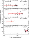 |
Fig. 3. Observed cyclotron line energy as a function of X-ray luminosity. Red data points denote the inverse-variance weighted average of the cyclotron line energy. Gray data points have been excluded from the averaging. The data for the top three panels have been collected by Staubert et al. (2019) and stem from Caballero et al. (2007), Sartore et al. (2015) and Fürst et al. (2015). The data for the bottom panel have been directly obtained from Chen et al. (2021). |
In Fig. 4, we depict the variation of the cyclotron line energy versus the measured intersection energy, for the four sources. The data suggest a positive correlation between the two quantities. The corresponding data is given in Table 1. As both Eint and ECRSF are subject to statistical and systematic uncertainties, one cannot model their relation simply by fitting a model and minimizing the χ2 statistic as it does not take the uncertainty of the independent coordinate into account. Instead, we calculated the ratio between outburst cyclotron line energy and intersection energy for each of the four data points. The uncertainty is estimated via Gaussian error propagation. From the four ratios, we calculate the weighted average with the inverse variance of the ratios as weights. We obtained
 (5)
(5)
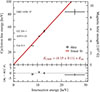 |
Fig. 4. Relation between magnetic field strength and intersection energy. Top panel: cyclotron line energies from literature versus intersection energies as obtained in this work. Black data points: sources with magnetic fields known from CRSF observations. Red line: linear regression taking uncertainties of ECRSF and Eint into account that is based on the four data points, with the relation is given in the lower right corner of the panel. Bottom panel: Residual of the best fit in units of the individual ratio uncertainty, σi. |
Outburst cyclotron line energies, intersection energies, and their ratio for the four sources with confirmed CRSFs.
One can make use of the relation between cyclotron line and magnetic field strength (see, e.g., Staubert et al. 2019, Eq. (1)) to express the magnetic field strength as a function of intersection energy as
 (6)
(6)
Further assuming a redshift of z = 0.24, which is expected for a 1.4 M⊙ neutron star with a radius of 12 km, we obtained
 (7)
(7)
For a canonical neutron star in a BeXRB system, the intersection energy in keV can therefore be roughly estimated as twice the magnetic field strength in units of 1012 G, which we designate as the 2-B-12 rule, analogous to the well-known 12-B-12 rule. In summary, we have shown that there exists a positive correlation between the surface magnetic field strength of neutron stars in BeXRBs and the intersection energy between the two spectral components present in their low-luminosity X-ray spectra.
3. Application of the doublehump model to simulated BeXRB spectra
The results presented in Sect. 2 indicate a positive correlation between magnetic field strength and intersection energy. In this section we show that such a correlation is also expected from a theoretical point of view. Specifically, from the growing number of physical spectral models for the quiescent state of BeXRBs (see, e.g., Mushtukov et al. 2021) we make use of the polar cap model (polcap hereafter) developed by Sokolova-Lapa et al. (2021). We introduce this model and its parameterization in Sect. 3.1 and show that the model indicates a relation between the hump position and the magnetic field. In Sect. 3.2 we then simulate NuSTAR observations based on this model and show that the relation between magnetic field strength and intersection energy is in qualitative agreement with our NuSTAR observations.
3.1. The polcap model
The polcap model (Sokolova-Lapa et al. 2021) is a theoretical spectral model that aims to reproduce the X-ray spectra of highly magnetized neutron stars at luminosities of 1033–1034 erg s−1. It is based on a numerical solution of the polarized radiative transfer equation, from which the resulting emergent spectrum is derived for a variety of magnetic field strengths and mass accretion rate configurations. The emergent spectra are tabulated for a range of configurations. In its current realization, the polcap model takes three input parameters:
-
the model normalization N, proportional to the ratio between the full area, onto which matter is being accreted that covers all polar caps, Aaccretion, and squared distance of the observer, D,
 (8)
(8) -
the logarithm of the area density of the mass flux accreted onto a single pole
![Mathematical equation: $$ \begin{aligned} \log \mathcal{F} _\mathrm{mass} \equiv \log \left[\left(\frac{\dot{M}}{1\,\mathrm{g} \,\mathrm{s} ^{-1}}\right)\cdot \left(\frac{A_\mathrm{cap} }{1\,\mathrm{cm} ^2}\right)^{-1}\right], \end{aligned} $$](/articles/aa/full_html/2026/05/aa58692-25/aa58692-25-eq10.gif) (9)
(9)which is the logarithm of the ratio between mass accretion rate and area of one polar cap, onto which the matter is accreted; and
-
the cyclotron energy, EcycNS, that is the energy where the cyclotron interaction cross section between photons and atmospheric electrons has its maximal value in the NS rest frame. The energy is naturally closely related to the cyclotron line energy of the observed absorption feature, which can be approximated by dividing the cyclotron energy by (1 + z) to compensate for the gravitational redshift. Where required, we convert the cyclotron energy to to the cyclotron line energy in the observer’s frame assuming a gravitational redshift of z = 0.24.
In order to demonstrate how the emergent spectrum changes with magnetic field strength, in Fig. 5 we show spectra computed with the polcap model for various magnetic field strengths (identified via the cyclotron energy in the NS frame). It is evident that the high-energy hump is shifted toward higher energies with increasing B-field strength, whereas the soft X-ray component shows a much weaker dependence on the magnetic field strength, which already suggests a positive correlation between the relative position of the two components and the magnetic field strength. Figure 5 also shows the NuSTAR effective area, which suggests that the HEC and the CRSF imprinted on it most likely cannot be resolved in typical cases where B ≳ a few 1012 G due to the rapidly decreasing effective area toward high energies.
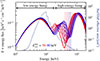 |
Fig. 5. Spectral model polcap for different magnetic field strengths. The magnetic field strengths are varied for cyclotron energies between 50–80 keV in the NS frame. The X-ray spectra are shown in the observer’s frame. The colored dashed lines indicate the cyclotron energy in the observer’s frame. The green line shows the NuSTAR effective area for a source region with 30″ diameter and 1′ off-axis angle. |
3.2. Simulations of X-ray spectra of BeXRBs at low luminosities
To study how the spectral changes with magnetic field predicted by the polcap models are reflected in observations, we simulated 100 ks NuSTAR observations of the spectra appropriate for BeXRBs located at a distance of 2 kpc and at an observed luminosity of 1034 erg s−1. The instrument response files and background spectra are taken from the 2022 NuSTAR observation of GX 304−1 (OBS ID 30701015002). The parameters of the polcap model are chosen as follows. The normalization is set such that the luminosity in the observer’s frame is 1034 erg s−1. We vary the mass flux over the whole tabulated range, that covers the whole range of values expected to prevail at low luminosities. The cyclotron energies are 50, 60, 70 and 80 keV in the NS rest frame, respectively, which covers the whole tabulated range.
We then fit the simulated spectra, rebinned to 30 counts per bin, with the doublehump model (see Fig. 6 for an example). As the doublehump model only describes the LEC and the red wing of the HEC, only data points up to 0.9 × Ecycobs are used to fit the model. The intersection energies obtained from the simulated spectra are shown as the dark green area in Fig. 7. To extrapolate toward higher magnetic field strengths than those tabulated for the polcap model (EcycNS = 80 keV, corresponding to ∼7 × 10¹² G), the left and right boundaries of the parameter space, that is the dark green area in Fig. 7, were fit with straight lines through the origin, whose slopes are mleft = 4.08 and mright = 3.52.
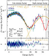 |
Fig. 6. Simulated NuSTAR spectrum based on the polcap model. Top panel: Simulated rebinned spectra in blue and teal for the two NuSTAR focal plane modules, respectively. The red line shows the polcap model, on which the simulated spectra are based. The input parameters are given in the lower left corner. Consistent with our treatment in Sect. 2, we base spectral fits only on data points sufficiently well below the CRSF energy, as the doublehump model does not account for CRSFs; data points not used spectral fitting are shown in gray. The fit doublehump model is shown in orange; its two cutoffpl components are shown as dashed orange lines. The cyclotron energy in observer’s rest frame is indicated by the black dashed line. Bottom panel: χ residuals of doublehump fit. |
3.3. Comparison between observations and theory
In the sections above we obtained relations between the relative position of the two spectral components, quantified as Eint, and the magnetic field strength in form of the cyclotron line energy from real observations and simulated spectra based on theoretical works, respectively. To compare the relations, we show the linear fit to the data points from real observations from Fig. 4 and the parameter space obtained from simulated spectra together in Fig. 7. The observation-driven relation from Sect. 2.4 and the theory-driven results both indicate a positive correlation between magnetic field strength and intersection energy. The data-driven relation is in good agreement with the left boundary of the parameter space given by the theory-driven approach.
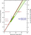 |
Fig. 7. Relation between magnetic field strength and intersection energy. Shown in red are the data points from real observations with the corresponding source names given on the left y-axis. The red line indicates the linear relation found in Sect. 2.4. The blue data points indicate the predicted magnetic field strengths for those BeXRBs without known magnetic field strength. Their names are given on the right y-axis. The solid green lines are obtained from the simulation-driven approach and resemble the left and right boundaries of the parameter space; the dashed green line show the behavior toward low B-field strengths, for which the polcap is not applicable due to spectral redistribution due to Landau excitations. The dark green area indicates the B-field range from which the green lines are obtained from; the light green area shows the extrapolation of the dark green area toward higher B-field strengths. |
Based on the data-driven linear correlation in Eqs. (5)–(7), we can also estimate the magnetic field strengths of the five BeXRBs studied in Sect. 2 for which no CRSFs have been claimed with high statistical significance, namely 2SXPS J075542.5−293353, IGR J21347+4737, MAXI J0655−013, SRGA J124404.1−632232 and X Per. The predicted values are shown in Fig. 7 as blue data points and are additionally listed in Table 2. While these values should be understood only as rough estimates of the magnetic field strength, based on a linear regression to only four data points with prior assumptions (see the discussion of applicability and limitations of the doublehump model in Sect. 4.2) they serve as testable hypotheses that are verifiable or falsifiable by deep observations of the hard X-ray band that could provide the statistics to find high-energy cyclotron lines.
Predicted magnetic field strengths and cyclotron line energies based on the observation-driven linear relation between intersection energy and cyclotron line energy and assuming z = 0.24.
4. Discussion
In this work, we have shown that the intersection energy between the two humps present in X-ray spectra of BeXRBs with luminosities of ∼1034 erg s−1 is correlated with the surface magnetic field strength inferred from CRSF observations. In this section we discuss the consequence of this result. We start in Sect. 4.1 with a discussion of the physical context. In Sect. 4.2, we discuss the applicability and limitations of the doublehump model and the linear correlation found in Sects. 2 and 3. In Sect. 4.3 we discuss and other possible tracers of the magnetic field strength in light of our findings. Given its pivotal role in recent history and its highly interesting spectrum, we discuss X Per individually in Sect. 4.4. Lastly, we outline possible next steps and give an outlook in Sect. 4.5.
4.1. Physical interpretation
Our study of real and simulated BeXRB observations at low luminosity has shown a positive correlation between the relative position of the two spectral components present in their X-ray spectra and the NS magnetic field strength. As theoretical models generally assume that the LEC depends much less on the magnetic field than the HEC (see Fig. 5 for the example of the polcap model), in the following we concentrate on the formation of the HEC.
In the model of Mushtukov et al. (2021), the HEC forms in an overheated atmosphere with an effective conversion of the kinetic energy of infalling matter to cyclotron photons. In this picture, the hump therefore consists of Comptonized cyclotron photons and is imprinted with a cyclotron (absorption) line that is due to inelastic scattering of cyclotron photons and electrons within the NS atmosphere. In this picture, the energy of the reprocessed cyclotron photons, and therefore the general position of the HEC, depends directly on the magnetic field strength.
Alternatively, Sokolova-Lapa et al. (2021) suggest that the HEC forms within the NS atmosphere, where initially ambient polarized soft X-ray photons are reprocessed in Compton interactions with infalling particles. These interactions increase the photon energy to tens of kiloelectronvolts. Cyclotron interactions that effectively remove photons with Eγ ∼ Ecyc alter the emergent spectral shape and imprint a deep absorption feature onto HEC. The cyclotron line itself is naturally related to the magnetic field strength. Therefore, the red wing of the CRSF, and, – although not observable – also its blue wing, are expected to depend on the magnetic field strength. In our empirical modeling attempt, we focus on the red wing and especially its rising flank to identify its intersection energy, which is subsequently also expected to depend on the magnetic field strength.
While these two theoretical frameworks utilize slightly different mechanisms for the formation of the HEC, both of them predict that the HEC location, and therefore also the intersection energy when the humps are modeled with the doublehump model, depends on the magnetic field. We directly demonstrated this for the physical model of Sokolova-Lapa et al. (2021) in Sect. 3.
It is noteworthy that already much earlier theoretical studies suggested that signatures of the strong magnetic field of ∼1012 G are present in the X-ray spectrum of HMXBs. Nelson et al. (1993) show that at least 10% of the accretion energy should be converted to radiation in the hard X-ray band at energies below the cyclotron line energy. They attribute this nonthermal emission to cyclotron photons, that are emitted in large numbers via the decay of electrons on higher Landau levels. In inelastic scattering, the cyclotron photons on average decrease their energy, which results in hard X-ray emission at energies below the cyclotron line energy. In a follow-up publication, Nelson et al. (1995) find that between 0.5% and 5% of the accretion luminosity is expected to be emitted as cyclotron emission between 5–20 keV. It is exactly this energy band that is crucial to determine the characteristics of the red wing of the HEC and the intersection energy of the two components. Depending on the assumed physical processes that lead to the formation of the HEC, this emission at intermediate energies could indeed be understood as the result of cyclotron emission.
4.2. The applicability of the doublehump model and our relation derived from it
The doublehump model itself is applicable to the X-ray spectra of BeXRBs with mass accretion rates low enough so that the accreted matter is not decelerated in a radiative shock, but within the NS atmosphere, such that double-humped X-ray spectra are formed. Unfortunately, it is not possible to give a simple luminosity threshold for its applicability. Instead, one needs to verify the presence of a hard X-ray component for example by applying a simpler cut off power law model; if a statistically significant excess at intermediate to high energies remains, this is an indicator that the spectrum potentially exhibits two distinct spectral components, in which case the doublehump model is applicable.
We emphasize that systems harboring rapidly rotating neutron stars, with periods on the order of a few seconds, are not expected to enter a state of low-level, stable accretion at luminosities of ∼1034 erg s−1. Rather, the rotating magnetic field is expected to inhibit accretion onto the NS (Campana et al. 2002). As a result, these objects are not expected to show a double-humped X-ray spectrum and are thought to enter a quiescent state (see, e.g., Rouco Escorial et al. 2020). Therefore, the doublehump model is not applicable to them.
The applicability of the doublehump model also depends on the magnetic field strength of the BeXRB in question. Due to the influence of Landau excitations which alter the spectral shape to a rather flat shape without two humps (see Gorban et al. 2022b, Fig. 5a) it is not valid for BeXRBs with field strengths below 2.5 × 10¹² G. In addition, as the doublehump model only describes the red wing of the HEC, it cannot model cyclotron lines and can therefore only be utilized for X-ray spectra up to the energies that are not affected by cyclotron interactions. As the cyclotron line begins to significantly alter the continuum for E ≳ 0.9 × ECRSFobs (see, e.g., Meszaros & Nagel 1985; Sokolova-Lapa et al. 2021), we use this threshold as the upper energy limit for modeling using the doublehump model.
Lastly, the spectral range of the data and the data’s level of constraint also impact the parameters of the doublehump model. For poor data the intersection energy is naturally less well constrained and is potentially correlated with the other doublehump parameters. For example, a preliminary study of MAXI J0655−013 has shown that the intersection energy decreases by 5 keV when utilizing well-constrained XMM-Newton data instead of poorly constrained Swift/XRT data along with NuSTAR data. While the value found using XMM-Newton is still within uncertainty of the Swift/XRT-derived value, this example shows that poor soft X-ray data can alter the modeling of the soft X-ray component and subsequently the intersection energy. It is therefore advisable to utilize NuSTAR in combination with highly sensitive soft X-ray instruments such as Chandra, NICER or XMM-Newton to achieve the most accurate spectral description possible.
4.3. Connecting the doublehump model and the magnetic field
In our empirical doublehump model, we have chosen to quantify the relative position of the two components via the intersection energy of the two cut off power laws utilized to describe the low-energy hump and the red wing of the high-energy hump. As described in Sect. 2.2, the reparametrization of the two cutoffpl components ensures that the components are forced to have an intersection point. This approach already constitutes a restriction of the spectral model that potentially eliminates a statistically more favorable description of the data, where the two components do not intersect.
The restriction to Γ2 = −2 for the component describing the HEC poses a further restriction for the model that is not necessarily required for those sources with high enough signal-to-noise ratio to constrain the falling flank toward the cyclotron line of the red wing sufficiently well. This is supported by directly fitting the polcap model spectra, where the HEC can be better constrained as its importance is not reduced by the rapidly declining effective area toward high energies present in real instruments. In this case we can constrain the full red wing of the HEC and generally find Γ2 < 0, which is not feasible for real or simulated NuSTAR spectra. As already touched upon in Sect. 2.2, the restriction also serves the purpose to achieve a description where each cut off power law component models each hump, respectively, instead of modeling both humps at the same time. To illustrate this, we show fits to the X-ray spectrum of X Per for a variety of fixed values of Γ2 in Fig. 8. Fits with negative Γ2 achieve the desired model description, where each cut off power law component models one spectral hump, whereas those with positive Γ2 achieve a favorable description only in a statistical sense, which nevertheless lacks physical interpretability. We therefore conducted our spectral analysis in this work with a fixed value of Γ2 = −2.
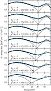 |
Fig. 8. Impact of Γ2 on spectral modeling. Each panel shows a fit to the X-ray spectrum of X Per (shown in blue and teal) with Γ2 fixed to the values given in the panels. The solid line shows the best-fit model, the dashed lines indicate the two model components, the vertical dotted lines indicate the resulting intersection energy. The χ2 statistic is given in each panel. |
While the intersection energy is arguably the most accessible parameter connecting the spectral shape and the magnetic field, as it only requires constraining the LEC and the rising flank of the HEC, other spectral parameters could in theory also be utilized. For example, the energy where the red wing of the HEC reaches its maximum value or the ratio between the maxima of the HEC and LEC should also be considered as tracers of the magnetic field. Both the position of the peak and the maximum flux value of the red wing of the HEC are inaccessible to NuSTAR at the typical magnetic field strengths considered here, B ≳ a few 1012 G. Moreover, the theoretical reasoning why the ratio between the maxima should be related to the magnetic field strength is challenging.
Other spectral parameters have already been shown to correlate with the NS magnetic field strength for HMXBs at much higher luminosities: Makishima et al. (1999) and Coburn et al. (2002) show that the cyclotron line energy is positively correlated with the spectral cut off energy. This correlation has also been found by the more recent study by Pradhan et al. (2021). Coburn et al. propose that this could indeed be a physical correlation between the B-field strength and the cut off energy. Alternatively, their positive correlation could also stem from a dependence of the cut off energy on the electron temperature, with the latter being potentially related to the magnetic field strength. The connection between Eint and magnetic field strength from this work on the other hand has a much more direct physical connection: the B-field dependence of the position of the HEC directly results in a measurable B-field dependence of the intersection energy.
4.4. The case of X Per
X Per is one of the most interesting sources touched upon in this work in many ways. First, it is the only persistent BeXRB in this work, whereas the other sources are transient sources, that are mostly only detectable during outbursts by monitors. Second, it is by far the closest source with a photo geometric distance of d ≈ 0.6 kpc (Bailer-Jones et al. 2021; Gaia Collaboration 2016, 2023). It is therefore also the source with the highest flux in our sample and its NuSTAR observation subsequently provides the highest signal-to-noise ratio. Third, X Per showcases how the scientific view of the quiescent state of BeXRBs has changed over the past 50 years. X Per was discovered by Giacconi et al. (1972) with the Uhuru satellite; its optical counterpart was identified as a Be star shortly thereafter (Moffat et al. 1973). White et al. (1976) first detected X-ray pulsations with a periodicity of 836 s. Around 20 years later, Di Salvo et al. (1998) report a 0.1–100 keV luminosity of ∼2.4 × 1034 erg s−1 based on a deep BeppoSAX observation. While they find that the soft X-ray spectrum is well-described by a cut off power law, a hard excess remains. Notably similar to the model utilized here, Di Salvo et al. describe the hard excess with a second cut off power law and theorize, motivated by Nelson et al. (1993), and Nelson et al. (1995), that the hard excess could be related to cyclotron emission. They approximate the cyclotron energy as the cut off energy of ∼65 keV, which yields a B-field strength of ∼5.6 × 10¹² G (see last paragraph of Sect. 4.3).
Shortly thereafter, Coburn et al. (2001) employ a model consisting of a blackbody and cut off power law component and report that a CRSF situated at ∼29 keV is required to obtain a satisfactory description of the RXTE data. This potential cyclotron line implies a magnetic field strength of ∼3 × 10¹² G. While the residuals of fits without the CRSF show a wave-like structure, this is only partly resolved by inclusion of the CRSF, which reduces the amplitude of the wave-like structure, but does not result in residuals statistically scattered around the zero-line (see Coburn et al. 2001, Fig. 4).
The claim of a ∼30 keV CRSF was reiterated by multiple later publications (e.g., Lutovinov et al. 2012; Rodi et al. 2024; Rai et al. 2025); however the evidence that the apparent absorption feature is in fact not caused by cyclotron resonant scattering has been growing for the past 15 years, starting with Doroshenko et al. (2012), who modeled the INTEGRAL spectrum of X Per with two Comptonizing plasma components (see Titarchuk 1994) and interpreted the observed dip at ∼30 keV as the dip between the two components and not as a cyclotron line. Based on the earlier timing analysis by Delgado-Martí et al. (2001) and the spin-down mechanism proposed by Illarionov & Kompaneets (1990), they estimated the magnetic field of X Per to be ∼1014 G, putting it within the range of magnetars (see, e.g., Olausen & Kaspi 2014). The application of the Ghosh & Lamb (1979) torque model by Yatabe et al. (2018) also yielded a value in excess of ∼1013 G. These measurements are further arguments against interpreting the feature at 30 keV as a CRSF, which would imply a field of B ∼ 3 × 10¹² G.
Moreover, the interpretation of the trough as the dip between the two spectral components has gained a much stronger theoretical foundation (Mushtukov et al. 2021; Sokolova-Lapa et al. 2021), as such dips are expected at energies of a few tens of keV. Recent IXPE observations of X Per reveal that it may be an orthogonal rotator and the results of Mushtukov et al. (2023) are generally in agreement with the theoretical studies of polarized emission at low luminosities (see, e.g., Mushtukov et al. 2021; Sokolova-Lapa et al. 2021, 2023a). While the direct confirmation of X Per’s strong magnetic field of ≳1013 G via CRSF detection above 100 keV is not feasible with the current generation of X-ray instruments, future missions with increased sensitivity in the hard X-ray band and soft Gamma-ray band may be able to achieve this goal. In this sense, X Per serves as an example that not all dips in the spectra of accreting neutron stars should automatically be interpreted as cyclotron lines.
4.5. Next steps and outlook
We have shown that the NS surface magnetic field strength is positively correlated with the intersection energy between the two spectral components of BeXRBs at low luminosities of ∼1034 erg s−1. Based on the availability of observations of sources with known B-field strength and the B-field range for which the polcap model has been tabulated for, we have investigated the relation for magnetic field strengths between a few 1012 G to approximately 1013 G, roughly covering half an order of magnitude.
To determine through observations whether this relation can be extended remains an interesting open question. This question can only be answered by obtaining BeXRB spectra at low luminosities with independently verified magnetic field strengths. Given the small number of accreting neutron stars in BeXRBs with known magnetic fields (see Staubert et al. 2019, Tables A1 and A2), extending our sample further is challenging. Observations during outbursts pose the potential to measure the magnetic field strength via CRSF identification, for example; observations during the decline of the outburst potentially allow study of the system at low mass accretion rates associated with the double-humped spectral shape. Each such pairing of measured magnetic field strength and observation during the low-luminosity state will help refine and possibly extend the validity of the linear relation probed here. All-sky surveys such as those of eROSITA (see, e.g., Predehl et al. 2021; Merloni et al. 2024) also have the potential to detect BeXRBs at low luminosities due to ever-increasing survey sensitivity.
Another interesting aspect to pursue is the pulse-phase resolved analysis at low luminosities, which could show whether the HEC changes as a function of pulse phase due to the varying viewing angle of the anisotropically emitting emission region. Analogous to the pulse-phase variability of CRSFs (see, e.g., Kreykenbohm et al. 2004; Staubert et al. 2019; Zalot et al. 2024), an investigation of the variability of the intersection energy could strengthen or weaken our results. However, exposure times well in excess of 100 ks would be required to study the phase-resolved spectra.
In parallel to these observational efforts, extensions of existing models are required to understand whether the relative position of the two components and the magnetic field strength are in fact linearly related for a larger range of B-field strengths.
Acknowledgments
We acknowledge partial funding from Deutsche Forschungsgemeinschaft under contract 414059771. This research was done under the auspices of DFG Forschungsgruppe 2290 (eRO-STEP). We acknowledge the pivotal contribution of Katja Pottschmidt to this project, the research of highly magnetized accreting neutron stars, and especially her mentoring of so many students and early-career scientists on both sides of the Atlantic. We deeply regret her untimely passing. We are committed to upholding her lasting legacy in new scientific frontiers. The authors thank Victoria Kaspi for her insight into SGR 0755−2933 and her helpful comments, Pragati Pradhan for her helpful comments, Rick Rothschild for his helpful comments on luminosity correlations, Rüdiger Staubert for providing us with cyclotron line energies that have been crucial for this work, Mihoko Yukita and the whole NuSTAR help desk for providing us with the names of observation PIs and the XMAG collaboration for productive discussions of this work. This research has made use of a collection of ISIS functions (ISISscripts) provided by ECAP/Remeis observatory and MIT (https://www.sternwarte.uni-erlangen.de/isis/), data and software provided by the High Energy Astrophysics Science Archive Research Center (HEASARC), which is a service of the Astrophysics Science Division at NASA/GSFC and data from the European Space Agency (ESA) mission Gaia (https://www.cosmos.esa.int/gaia), processed by the Gaia Data Processing and Analysis Consortium (DPAC, https://www.cosmos.esa.int/web/gaia/dpac/consortium). Funding for the DPAC has been provided by national institutions, in particular the institutions participating in the Gaia Multilateral Agreement.
References
- Araya, R. A., & Harding, A. K. 1999, ApJ, 517, 334 [NASA ADS] [CrossRef] [Google Scholar]
- Bailer-Jones, C. A. L., Rybizki, J., Fouesneau, M., Demleitner, M., & Andrae, R. 2021, AJ, 161, 147 [Google Scholar]
- Ballhausen, R., Pottschmidt, K., Fürst, F., et al. 2017, A&A, 608, A105 [NASA ADS] [CrossRef] [EDP Sciences] [Google Scholar]
- Barthelmy, S. D., D’Elia, V., Gehrels, N., et al. 2016, ATel, 8831 [Google Scholar]
- Basko, M. M., & Sunyaev, R. A. 1975, A&A, 42, 311 [NASA ADS] [Google Scholar]
- Basko, M. M., & Sunyaev, R. A. 1976, MNRAS, 175, 395 [Google Scholar]
- Becker, P. A., Klochkov, D., Schönherr, G., et al. 2012, A&A, 544, A123 [NASA ADS] [CrossRef] [EDP Sciences] [Google Scholar]
- Brumback, M. C., Hickox, R. C., Fürst, F. S., et al. 2018, ApJ, 852, 132 [Google Scholar]
- Burrows, D. N., Hill, J. E., Nousek, J. A., et al. 2005, Space Sci. Rev., 120, 165 [Google Scholar]
- Caballero, I., Kretschmar, P., Santangelo, A., et al. 2007, A&A, 465, L21 [NASA ADS] [CrossRef] [EDP Sciences] [Google Scholar]
- Campana, S., Stella, L., Israel, G. L., et al. 2002, ApJ, 580, 389 [NASA ADS] [CrossRef] [Google Scholar]
- Chaty, S. 2011, ASP Conf. Proc., 447, 29 [Google Scholar]
- Chen, X., Wang, W., Tang, Y. M., et al. 2021, ApJ, 919, 33 [CrossRef] [Google Scholar]
- Coburn, W., Heindl, W. A., Gruber, D. E., et al. 2001, ApJ, 552, 738 [NASA ADS] [CrossRef] [Google Scholar]
- Coburn, W., Heindl, W. A., Rothschild, R. E., et al. 2002, ApJ, 580, 394 [NASA ADS] [CrossRef] [Google Scholar]
- Delgado-Martí, H., Levine, A. M., Pfahl, E., & Rappaport, S. A. 2001, ApJ, 546, 455 [CrossRef] [Google Scholar]
- den Herder, J. W., Brinkman, A. C., Kahn, S. M., et al. 2001, A&A, 365, L7 [NASA ADS] [CrossRef] [EDP Sciences] [Google Scholar]
- Di Salvo, T., Burderi, L., Robba, N. R., & Guainazzi, M. 1998, ApJ, 509, 897 [NASA ADS] [CrossRef] [Google Scholar]
- Doroshenko, V., Santangelo, A., Kreykenbohm, I., & Doroshenko, R. 2012, A&A, 540, L1 [NASA ADS] [CrossRef] [EDP Sciences] [Google Scholar]
- Doroshenko, V., Santangelo, A., Tsygankov, S. S., & Ji, L. 2021, A&A, 647, A165 [NASA ADS] [CrossRef] [EDP Sciences] [Google Scholar]
- Doroshenko, V., Staubert, R., Maitra, C., et al. 2022, A&A, 661, A21 [NASA ADS] [CrossRef] [EDP Sciences] [Google Scholar]
- Finger, M. H., Cominsky, L. R., Wilson, R. B., Harmon, B. A., & Fishman, G. J. 1994, AIP Conf. Proc., 308, 459 [Google Scholar]
- Fürst, F., Pottschmidt, K., Miyasaka, H., et al. 2015, ApJ, 806, L24 [CrossRef] [Google Scholar]
- Fürst, F., Falkner, S., Marcu-Cheatham, D., et al. 2018, A&A, 620, A153 [NASA ADS] [CrossRef] [EDP Sciences] [Google Scholar]
- Gaia Collaboration. 2016, A&A, 595, A1 [NASA ADS] [CrossRef] [EDP Sciences] [Google Scholar]
- Gaia Collaboration. 2023, A&A, 674, A1 [NASA ADS] [CrossRef] [EDP Sciences] [Google Scholar]
- Gehrels, N., Chincarini, G., Giommi, P., et al. 2004, ApJ, 611, 1005 [Google Scholar]
- Gendreau, K. C., Arzoumanian, Z., & Okajima, T. 2012, in Space Telescopes and Instrumentation 2012: Ultraviolet to Gamma Ray, eds. T. Takahashi, S. S. Murray, & J.-W. A. den Herder, (SPIE), 8443, 322 [Google Scholar]
- Gendreau, K. C., Arzoumanian, Z., Adkins, P. W., et al. 2016, in Space Telescopes and Instrumentation 2016: Ultraviolet to Gamma Ray, eds. J.-W. A. den Herder, T. Takahashi, & M. Bautz, (SPIE), 9905, 420 [Google Scholar]
- Ghimiray, M., Sharma, P., & Subba, N. 2024, MNRAS, 531, 3386 [Google Scholar]
- Ghising, M., Tamang, R., Rai, B., Tobrej, M., & Paul, B. C. 2023, J. Astrophys. Astr., 44, 94 [Google Scholar]
- Ghosh, P., & Lamb, F. K. 1979, ApJ, 234, 296 [Google Scholar]
- Giacconi, R., Murray, S., Gursky, H., et al. 1972, ApJ, 178, 281 [NASA ADS] [CrossRef] [Google Scholar]
- Gorban, A. S., Molkov, S. V., Lutovinov, A. A., & Semena, A. N. 2022a, Astron. Lett., 48, 798 [Google Scholar]
- Gorban, A. S., Molkov, S. V., Tsygankov, S. S., Mushtukov, A. A., & Lutovinov, A. A. 2022b, Astron. Lett., 48, 256 [Google Scholar]
- Harding, A. K., & Lai, D. 2006, RPPh, 69, 2631 [Google Scholar]
- Harding, A. K., Meszaros, P., Kirk, J. G., & Galloway, D. J. 1984, ApJ, 278, 369 [CrossRef] [Google Scholar]
- Harrison, A., & Lynch, R. 2017, AAS Meeting #229, Id.431.04 (Grapevine, Texas: American Astronomical Society) [Google Scholar]
- Harrison, F. A., Craig, W. W., Christensen, F. E., et al. 2013, ApJ, 770, 103 [Google Scholar]
- HI4PI Collaboration (Ben Bekhti, N., et al.) 2016, A&A, 594, A116 [NASA ADS] [CrossRef] [EDP Sciences] [Google Scholar]
- Houck, J. C., & Denicola, L. A. 2000, ASP Conf. Ser., 216, 591 [Google Scholar]
- Illarionov, A. F., & Kompaneets, D. A. 1990, MNRAS, 247, 219 [NASA ADS] [Google Scholar]
- Jansen, F., Lumb, D., Altieri, B., et al. 2001, A&A, 365, L1 [NASA ADS] [CrossRef] [EDP Sciences] [Google Scholar]
- Kreykenbohm, I., Wilms, J., Coburn, W., et al. 2004, A&A, 427, 975 [NASA ADS] [CrossRef] [EDP Sciences] [Google Scholar]
- Krivonos, R. A., Tsygankov, S. S., Lutovinov, A. A., et al. 2015, ApJ, 809, 140 [NASA ADS] [CrossRef] [Google Scholar]
- Kühnel, M., Müller, S., Kreykenbohm, I., et al. 2013, A&A, 555, A95 [NASA ADS] [CrossRef] [EDP Sciences] [Google Scholar]
- Lamb, F. K., Pethick, C. J., & Pines, D. 1973, ApJ, 184, 271 [NASA ADS] [CrossRef] [Google Scholar]
- Ludlam, R. M., Grefenstette, B. W., Brumback, M. C., et al. 2022, ApJ, 934, 59 [Google Scholar]
- Lutovinov, A., Tsygankov, S., & Chernyakova, M. 2012, MNRAS, 423, 1978 [NASA ADS] [CrossRef] [Google Scholar]
- Lutovinov, A. A., Tsygankov, S. S., Postnov, K. A., et al. 2017, MNRAS, 466, 593 [Google Scholar]
- Lutovinov, A., Tsygankov, S., Molkov, S., et al. 2021, ApJ, 912, 17 [Google Scholar]
- Makishima, K., Mihara, T., Nagase, F., & Tanaka, Y. 1999, ApJ, 525, 978 [NASA ADS] [CrossRef] [Google Scholar]
- Malacaria, C., Klochkov, D., Santangelo, A., & Staubert, R. 2015, A&A, 581, A121 [NASA ADS] [CrossRef] [EDP Sciences] [Google Scholar]
- Malacaria, C., Pike, S. N., D’Aì, A., et al. 2026, A&A, 706, A321 [NASA ADS] [CrossRef] [EDP Sciences] [Google Scholar]
- Markwardt, C., Arzoumanian, Z., Gendreau, K., Hare, J., & NICER Team. 2024, in Bulletin of the American Astronomical Society, eds. E. Vishniac, & A. Muench, 56 (Washington, DC: AAS Publishing) [Google Scholar]
- McBride, V. A., Wilms, J., Kreykenbohm, I., et al. 2007, A&A, 470, 1065 [NASA ADS] [CrossRef] [EDP Sciences] [Google Scholar]
- Merloni, A., Lamer, G., Liu, T., et al. 2024, A&A, 682, A34 [NASA ADS] [CrossRef] [EDP Sciences] [Google Scholar]
- Meszaros, P., & Nagel, W. 1985, ApJ, 299, 138 [NASA ADS] [CrossRef] [Google Scholar]
- Meszaros, P., Harding, A. K., Kirk, J. G., & Galloway, D. J. 1983, ApJ, 266, L33 [Google Scholar]
- Miller, G. S., Salpeter, E. E., & Wasserman, I. 1987, ApJ, 314, 215 [Google Scholar]
- Miller, G., Wasserman, I., & Salpeter, E. E. 1989, ApJ, 346, 405 [Google Scholar]
- Mitsuda, K., Inoue, H., Koyama, K., et al. 1984, PASJ, 36, 741 [NASA ADS] [Google Scholar]
- Moffat, A. F. J., Haupt, W., & Schmidt-Kaler, T. 1973, A&A, 23, 433 [Google Scholar]
- Mroz, P., & Udalski, A. 2021, ATel, 14361 [Google Scholar]
- Mushtukov, A. A., Suleimanov, V. F., Tsygankov, S. S., & Poutanen, J. 2015, MNRAS, 447, 1847 [NASA ADS] [CrossRef] [Google Scholar]
- Mushtukov, A. A., Suleimanov, V. F., Tsygankov, S. S., & Portegies Zwart, S. 2021, MNRAS, 503, 5193 [Google Scholar]
- Mushtukov, A. A., Tsygankov, S. S., Poutanen, J., et al. 2023, MNRAS, 524, 2004 [NASA ADS] [CrossRef] [Google Scholar]
- Nagel, W. 1981, ApJ, 251, 288 [Google Scholar]
- NASA HEASARC. 2014, ASCL, 1408, 004 [Google Scholar]
- Nelson, R. W., Salpeter, E. E., & Wasserman, I. 1993, ApJ, 418, 874 [Google Scholar]
- Nelson, R. W., Wang, J. C. L., Salpeter, E. E., & Wasserman, I. 1995, ApJ, 438, L99 [Google Scholar]
- Olausen, S. A., & Kaspi, V. M. 2014, ApJS, 212, 6 [Google Scholar]
- Orlandini, M., & Fiume, D. D. 2001, AIP Conf. Proc., 599, 283 [Google Scholar]
- Pike, S. N., Sugizaki, M., van den Eijnden, J., et al. 2023, ApJ, 954, 48 [Google Scholar]
- Pradhan, P., Paul, B., Bozzo, E., Maitra, C., & Paul, B. C. 2021, MNRAS, 502, 1163 [NASA ADS] [CrossRef] [Google Scholar]
- Predehl, P., Andritschke, R., Arefiev, V., et al. 2021, A&A, 647, A1 [EDP Sciences] [Google Scholar]
- Rai, B., Tobrej, M., Ghising, M., Tamang, R., & Paul, B. C. 2023, MNRAS, 524, 1352 [Google Scholar]
- Rai, B., Tobrej, M., Ghising, M., & Paul, B. C. 2025, JHEAP, 45, 265 [Google Scholar]
- Raman, G., Varun, Pradhan, P., & Kennea, J. 2023, MNRAS, 526, 3262 [Google Scholar]
- Rodi, J., Natalucci, L., & Fiocchi, M. 2024, A&A, 689, A186 [NASA ADS] [CrossRef] [EDP Sciences] [Google Scholar]
- Rouco Escorial, A., van den Eijnden, J., & Wijnands, R. 2018, A&A, 620, L13 [NASA ADS] [CrossRef] [EDP Sciences] [Google Scholar]
- Rouco Escorial, A., Wijnands, R., van den Eijnden, J., et al. 2020, A&A, 638, A152 [NASA ADS] [CrossRef] [EDP Sciences] [Google Scholar]
- Salganik, A., Tsygankov, S. S., Doroshenko, V., et al. 2023, MNRAS, 524, 5213 [NASA ADS] [CrossRef] [Google Scholar]
- Salganik, A., Tsygankov, S. S., Chernyakova, M., Malyshev, D., & Poutanen, J. 2025, A&A, 698, A71 [NASA ADS] [CrossRef] [EDP Sciences] [Google Scholar]
- Sartore, N., Jourdain, E., & Roques, J. P. 2015, ApJ, 806, 193 [NASA ADS] [CrossRef] [Google Scholar]
- Sokolova-Lapa, E., Gornostaev, M., Wilms, J., et al. 2021, A&A, 651, A12 [NASA ADS] [CrossRef] [EDP Sciences] [Google Scholar]
- Sokolova-Lapa, E., Stierhof, J., Dauser, T., & Wilms, J. 2023a, A&A, 674, L2 [NASA ADS] [CrossRef] [EDP Sciences] [Google Scholar]
- Sokolova-Lapa, E., Zalot, N., Stierhof, J., et al. 2023b, ATel, 16171 [Google Scholar]
- Staubert, R., Trümper, J., Kendziorra, E., et al. 2019, A&A, 622, A61 [NASA ADS] [CrossRef] [EDP Sciences] [Google Scholar]
- Strüder, L., Briel, U., Dennerl, K., et al. 2001, A&A, 365, L18 [Google Scholar]
- Sugizaki, M., Yamamoto, T., Mihara, T., Nakajima, M., & Makishima, K. 2015, PASJ, 67, 73 [NASA ADS] [Google Scholar]
- Thompson, C., & Duncan, R. C. 1995, MNRAS, 275, 255 [Google Scholar]
- Titarchuk, L. 1994, ApJ, 434, 570 [NASA ADS] [CrossRef] [Google Scholar]
- Tsygankov, S. S., Doroshenko, V., Mushtukov, A. A., Lutovinov, A. A., & Poutanen, J. 2019a, MNRAS, 487, L30 [Google Scholar]
- Tsygankov, S. S., Rouco Escorial, A., Suleimanov, V. F., et al. 2019b, MNRAS, 483, L144 [NASA ADS] [CrossRef] [Google Scholar]
- Turner, M. J. L., Abbey, A., Arnaud, M., et al. 2001, A&A, 365, L27 [CrossRef] [EDP Sciences] [Google Scholar]
- Verner, D. A., Ferland, G. J., Korista, K. T., & Yakovlev, D. G. 1996, ApJ, 465, 487 [Google Scholar]
- Vybornov, V., Klochkov, D., Gornostaev, M., et al. 2017, A&A, 601, A126 [NASA ADS] [CrossRef] [EDP Sciences] [Google Scholar]
- Weisskopf, M. C., Tananbaum, H. D., Van Speybroeck, L. P., & O’Dell, S. L. 2000, Proc. SPIE, 4012, 2 [Google Scholar]
- White, N. E., Mason, K. O., Sanford, P. W., & Murdin, P. 1976, MNRAS, 176, 201 [NASA ADS] [Google Scholar]
- Wilms, J., Allen, A., & McCray, R. 2000, ApJ, 542, 914 [Google Scholar]
- Yamamoto, T., Sugizaki, M., Mihara, T., et al. 2011, PASJ, 63, S751 [Google Scholar]
- Yatabe, F., Makishima, K., Mihara, T., et al. 2018, PASJ, 70, 89 [Google Scholar]
- Zalot, N., Sokolova-Lapa, E., Stierhof, J., et al. 2024, A&A, 686, A95 [NASA ADS] [CrossRef] [EDP Sciences] [Google Scholar]
- Zel’dovich, Ya. B., & Shakura, N. I. 1969, SvA, 13, 175 [Google Scholar]
This object was initially detected and classified as a soft gamma repeater (Barthelmy et al. 2016) under the name SGR 0755−2933. Magnetars are known to exhibit bursts associated with crust fractures (Thompson & Duncan 1995). Doroshenko et al. (2021) show concrete evidence for pulsations, which were also already hinted at by Harrison & Lynch (2017). The former argue that the X-ray source observed by NuSTAR is most likely not the counterpart of the burst and is actually a BeXRB, which they refer to as 2SXPS J075542.5−293353.
For transparency, in Fig. 2 we nevertheless show the spectral fit for the full NuSTAR energy range, coloring data points that have not been included in the fit in gray.
Appendix A: Data extraction and reduction
In this section we document our data extraction procedure. All extractions are conducted with HEAsoft version 6.36 (NASA HEASARC 2014), all subsequent spectral analysis is conducted with ISIS version 1.6.2 (Houck & Denicola 2000). All spectra are rebinned based on a minimum counts per bin criterion, whose threshold value is set manually for each source and instrument depending on the count rate.
A.1. NuSTAR
NuSTAR datasets are reprocessed using NuSTAR pipeline version 0.4.12. For each focal plane module, source and background regions are chosen as circles and annuli, respectively. Both the source and background regions are centered on the point source. As the observations cover a wide range of source fluxes, the source region circle radii are chosen individually for each observation. The background region annuli radii are chosen such that they cover as much of the detector area as possible in order to constrain the background emission as precisely as possible. A potential drawback of this method is that the detector response is not uniform over the full detector area. For SRGA J124404.1−632232, we instead chose four circular regions as the background region, as the observation was significantly affected by stray light (Ludlam et al. 2022).
We extract X-ray spectra using NuSTARDAS version 2.1.5. Unless given otherwise in Sect. 2.3, we make use of the full NuSTAR energy range of 3.5–79 keV.
A.2. Chandra
Chandra data are extracted using CIAO version 4.17. The source and background regions are circular regions.
A.3. NICER
NICER/XTI data are extracted using the nicerl3 version 1.14 routines. We utilize the SCORPEON background model (Markwardt et al. 2024).
A.4. Swift
Swift/XRT data are extracted using the xrtpipeline version 0.13.7. Source and background regions are chosen as circles and annuli around the point sources, respectively.
A.5. XMM-Newton
XMM-Newton data are extracted using the Science Analysis System (SAS) version 22.1.0. Source and background regions are circular, where the source region radius depends on the source flux and the background source region is set to 60". Flaring particle background was taken into account by visual inspection of the 10–12 keV light curve; time intervals with visible spikes in count rate have been discarded. Additionally, a significant portion of the XMM-Newton observation of MAXI J0655−013 had to be discarded to to solar activity.
Appendix B: Source overview and spectral parameters
Overview of observations and spectral models utilized in this work. Upper part of the table: source and observation information. Lower part of the table: parameters of doublehump spectral fits shown in Fig. 2.
All Tables
Outburst cyclotron line energies, intersection energies, and their ratio for the four sources with confirmed CRSFs.
Predicted magnetic field strengths and cyclotron line energies based on the observation-driven linear relation between intersection energy and cyclotron line energy and assuming z = 0.24.
Overview of observations and spectral models utilized in this work. Upper part of the table: source and observation information. Lower part of the table: parameters of doublehump spectral fits shown in Fig. 2.
All Figures
|
Fig. 1. NuSTAR X-ray spectra of BeXRBs in quiescence. The spectra are ordered by decreasing energy at which the hard X-ray-component peaks, from top to bottom. The respective rescaling factors, where required, are given next to the source names. |
| In the text | |
|
Fig. 2. Spectral fit of the doublehump model to quiescent X-ray spectra of nine BeXRBs. Left panel: Unfolded E × FE spectra and fit model (solid line); the dashed lines indicate the two components of the doublehump model. The spectra are separated vertically for improved perceptibility, ordered by descending intersection energy from top to bottom, and to this end have been rescaled by the factors given on the left y-axis of the left panel. The spectra have also been rescaled to match NuSTAR/FPMA according to the cross-calibration constants. Right panel: χ residuals of spectral fits for each source, respectively. The gray residuals indicate data points that were not used for spectral fitting, as they are at or above the CRSF feature, which is not part of the doublehump model and therefore excluded. The spectra have been rebinned and the NuSTAR FPMs combined for visual purposes. |
| In the text | |
|
Fig. 3. Observed cyclotron line energy as a function of X-ray luminosity. Red data points denote the inverse-variance weighted average of the cyclotron line energy. Gray data points have been excluded from the averaging. The data for the top three panels have been collected by Staubert et al. (2019) and stem from Caballero et al. (2007), Sartore et al. (2015) and Fürst et al. (2015). The data for the bottom panel have been directly obtained from Chen et al. (2021). |
| In the text | |
|
Fig. 4. Relation between magnetic field strength and intersection energy. Top panel: cyclotron line energies from literature versus intersection energies as obtained in this work. Black data points: sources with magnetic fields known from CRSF observations. Red line: linear regression taking uncertainties of ECRSF and Eint into account that is based on the four data points, with the relation is given in the lower right corner of the panel. Bottom panel: Residual of the best fit in units of the individual ratio uncertainty, σi. |
| In the text | |
|
Fig. 5. Spectral model polcap for different magnetic field strengths. The magnetic field strengths are varied for cyclotron energies between 50–80 keV in the NS frame. The X-ray spectra are shown in the observer’s frame. The colored dashed lines indicate the cyclotron energy in the observer’s frame. The green line shows the NuSTAR effective area for a source region with 30″ diameter and 1′ off-axis angle. |
| In the text | |
|
Fig. 6. Simulated NuSTAR spectrum based on the polcap model. Top panel: Simulated rebinned spectra in blue and teal for the two NuSTAR focal plane modules, respectively. The red line shows the polcap model, on which the simulated spectra are based. The input parameters are given in the lower left corner. Consistent with our treatment in Sect. 2, we base spectral fits only on data points sufficiently well below the CRSF energy, as the doublehump model does not account for CRSFs; data points not used spectral fitting are shown in gray. The fit doublehump model is shown in orange; its two cutoffpl components are shown as dashed orange lines. The cyclotron energy in observer’s rest frame is indicated by the black dashed line. Bottom panel: χ residuals of doublehump fit. |
| In the text | |
|
Fig. 7. Relation between magnetic field strength and intersection energy. Shown in red are the data points from real observations with the corresponding source names given on the left y-axis. The red line indicates the linear relation found in Sect. 2.4. The blue data points indicate the predicted magnetic field strengths for those BeXRBs without known magnetic field strength. Their names are given on the right y-axis. The solid green lines are obtained from the simulation-driven approach and resemble the left and right boundaries of the parameter space; the dashed green line show the behavior toward low B-field strengths, for which the polcap is not applicable due to spectral redistribution due to Landau excitations. The dark green area indicates the B-field range from which the green lines are obtained from; the light green area shows the extrapolation of the dark green area toward higher B-field strengths. |
| In the text | |
|
Fig. 8. Impact of Γ2 on spectral modeling. Each panel shows a fit to the X-ray spectrum of X Per (shown in blue and teal) with Γ2 fixed to the values given in the panels. The solid line shows the best-fit model, the dashed lines indicate the two model components, the vertical dotted lines indicate the resulting intersection energy. The χ2 statistic is given in each panel. |
| In the text | |
Current usage metrics show cumulative count of Article Views (full-text article views including HTML views, PDF and ePub downloads, according to the available data) and Abstracts Views on Vision4Press platform.
Data correspond to usage on the plateform after 2015. The current usage metrics is available 48-96 hours after online publication and is updated daily on week days.
Initial download of the metrics may take a while.