| Issue |
A&A
Volume 709, May 2026
|
|
|---|---|---|
| Article Number | A192 | |
| Number of page(s) | 8 | |
| Section | Extragalactic astronomy | |
| DOI | https://doi.org/10.1051/0004-6361/202558540 | |
| Published online | 13 May 2026 | |
Spectral index evolution of the limb-brightened jet in 3C 84
1
Max-Planck-Institut für Radioastronomie, Auf dem Hügel 69, D-53121 Bonn, Germany
2
Finnish Centre for Astronomy with ESO, University of Turku, 20014 Turku, Finland
3
Aalto University Metsähovi Radio Observatory, Metsähovintie 114, FI-02540 Kylmälä, Finland
4
Center for Astrophysics | Harvard & Smithsonian, 60 Garden Street, Cambridge, Massachusetts 02138, USA
5
Dept. of Physics & Astronomy, Sejong University, Guangjin-gu, Seoul 05006, Republic of Korea
6
Department of Astrophysics, Institute for Mathematics, Astrophysics and Particle Physics (IMAPP), Radboud University, P.O. Box 9010, 6500 GL Nijmegen, The Netherlands
7
Department of Physics, Ulsan National Institute of Science and Technology, 50 UNIST-gil, Eonyang-eup, Ulju-gun, Ulsan 44919, Republic of Korea
8
Instituto de Física, Pontificia Universidad Católica de Valparaíso, Casilla 4059 Valparaíso, Chile
9
Department of Physics and Astronomy, University of Mississippi, University, Mississippi 38677, USA
10
Astronomy Department, Universidad de Concepción, Casilla 160-C, Concepción, Chile
11
Joint Institute for VLBI ERIC (JIVE), Oude Hoogeveensedijk 4, 7991 PD Dwingeloo, The Netherlands
★ Corresponding author: This email address is being protected from spambots. You need JavaScript enabled to view it.
Received:
12
December
2025
Accepted:
13
April
2026
Abstract
Relativistic jets launched by active galactic nuclei are fundamental for understanding the physics of accreting supermassive black holes and their immediate environment, but the mechanisms that drive the jet launching remain uncertain. We investigate the sub-parsec jet of 3C 84 using multi-epoch multi-frequency very long baseline interferometry (VLBI) observations with the European VLBI Network and the Very Long Baseline Array at 22 and 43 GHz. We analysed the evolution of the spectral index gradient in the core region to relate the observed structure to physical interpretations and to distinguish between competing jet-launching models. Furthermore, we examined the effect of the ambient medium and magnetic field configuration on the jet morphology and dynamics over time and explored their connection to a coinciding γ-ray flare. Our spectral analysis reveals significant changes across three epochs, indicating dynamic activity between filamentary structures on sub-parsec scales, evolving magnetic fields, and a complex interaction with the surrounding medium, all of which shape the innermost jet and might affect its high-energy emission.
Key words: instrumentation: high angular resolution / instrumentation: interferometers / galaxies: active / galaxies: jets / quasars: individual: 3C 84
© The Authors 2026
 Open Access article, published by EDP Sciences, under the terms of the Creative Commons Attribution License (https://creativecommons.org/licenses/by/4.0), which permits unrestricted use, distribution, and reproduction in any medium, provided the original work is properly cited.
This article is published in open access under the Subscribe to Open model.
Open access funding provided by Max Planck Society.
1. Introduction
Relativistic jets in active galactic nuclei (AGNs) are highly collimated and energetic outflows of plasma, emanating from the vicinity of the central engine. Until today, the exact launching process of relativistic jets remains a subject of investigation. The launching mechanism postulated by Blandford & Znajek (1977), the BZ process hereafter, suggests that rotational energy is directly extracted from the central black hole, launching a jet close to the central engine. In contrast, Blandford & Payne (1982; BP process) predicts that rotational energy is extracted from the accretion disc, powering a jet that has a wider and stratified jet base. However, these two mechanisms are not mutually exclusive and may coexist and might contribute jointly to the observed jet structure. AGN jets have been widely tested for these mechanisms, in which a more collimated jet indicates the presence of the BZ process (see Walker et al. 2018; Lu et al. 2023, for a review), while a wider jet would favour the BP mechanism (Giovannini et al. 2018; Paraschos et al. 2024b). Since these two launching models result from a substantially different magnetic field configuration and jet geometry, they can be distinguished by studying the innermost jet region of nearby AGNs. Very long baseline interferometry (VLBI) observations at centimetre and millimetre wavelengths provide a high angular resolution that is essential for probing the innermost regions of AGN jets, where jet collimation takes place (see Boccardi et al. 2021, for more details).
3C 84 is a compact radio source in the central galaxy NGC 1275 of the Perseus cluster. Its proximity at redshift z = 0.018 (Strauss et al. 1992), its brightness and jet structure make it a prime target for testing jet-launching scenarios, as well as studying the innermost sub-parsec AGN structure (Walker et al. 2000; Kam et al. 2024). Previous VLBI studies revealed a complex jet morphology in the sub-milliarcseond region: Paraschos et al. (2022b) observed a time-varying spectral index gradient in the innermost jet (2011–2020), attributed to structural variability, while Park et al. (2024) reported transverse limb-brightening gradients with inverted-edge spectra, indicating complex interactions with the ambient medium. Nagai et al. (2014), Giovannini et al. (2018), Kim et al. (2019), and Paraschos et al. (2024a) found evidence of a limb-brightened structure in total intensity and in linear polarisation, whereby the edge appears brighter than the spine. This is consistent with a stratified jet, a velocity or magnetic field gradient, or a combination of the two (for a detailed review see Blandford et al. 2019). These filamentary structures that start from the core region are collimated and elongated patterns of enhanced emission. They extend into farther downstream into the jet (Nagai et al. 2014; Giovannini et al. 2018; Punsly et al. 2021). Paraschos & Mpisketzis (2025) investigated these filaments close to the central engine using centimetre-VLBI observations and found that their morphology might arise from Kelvin-Helmholtz (K-H) instabilities, driven by interactions between the jet plasma and the ambient medium (Fuentes et al. 2023; Nikonov et al. 2023). Additionally, 3C 84 shows strong γ-ray variability (Nagai et al. 2012; Hodgson et al. 2021). Previously, the ejection of new components in 3C 84 was linked to subsequent γ-ray flares (Paraschos et al. 2022b, 2023; Hodgson et al. 2021), with a delayed flare peak, but the spatial origin of γ rays in this source is thought to be diverse in the VLBI core and the downstream jet, where the jet shows signatures of strong interaction with the interstellar medium.
We investigate a possible connection between the observed limb-brightening and the variability in the γ-ray regime by probing the innermost structures with multi-epoch, multi-frequency VLBI observations of 3C 84. In particular, we examined whether the spectral index distribution within the jet of 3C 84 also exhibits limb-brightened features similar to the electric vector position angle (EVPA) patterns observed in the linear polarisation strength of the jet (as seen in Paraschos et al. 2024a). Moreover, we imaged the sub-parsec scale region to map the spectral index gradient, which provided insights into the distinction of different jet-launching models (Paraschos et al. 2022a). Leveraging the increased sensitivity of our latest VLBI datasets, we examined temporal changes in the spectral index with high precision to identify signatures of synchrotron emission, absorption, and particle acceleration, thereby providing possible explanations for the jet morphology and its interaction with the surrounding medium. We further compared radio and γ-ray light curves to link changes in high-energy emission to structural and spectral variations, providing insights into the connection between flaring events and the jet-launching region.
This paper is structured as follows: In Sect. 2 we provide information about the observations and data reduction. Section 3 outlines the methods and presents the results. In Sect. 4 we discuss our results, and in Sect. 5 we draw conclusions of our analysis. Throughout this paper, we assume a Λ cold dark matter cosmology with H0 = 67.8 km s−1 Mpc−1, ΩΛ = 0.692, and Ωm = 0.308 (Planck Collaboration XIII 2016), so that 1 mas corresponds to 0.37 pc.
2. Observations and data reduction
3C 84 was observed by the European VLBI Network (EVN) in June 2024 and November 2021 at 22 and 43 GHz, supplemented by observations by the Very Long Baseline Array (VLBA) and the Global VLBI Alliance (GVA) in 2022 at the same frequencies. Because observational issues affected the 43 GHz data from 2021 on long baselines, we used data available from the VLBA-BU Blazar Monitoring Program (BEAM-ME and VLBA-BU-BLAZAR1). The data from observations in 2021, 2022, and 2024 were recorded in eight baseband channels for each frequency with two-bit quantisation and a sample rate of 2 Gbps for all but the Australian Long Baseline Array (LBA) in 2022 (1 Gbps). Finally, the data of 2021, 2022, and 2024 were correlated at the correlator at the Joint Institute for Very Long Baseline Interferometry European Research Infrastructure Consortium (JIVE) in Dwingeloo, Netherlands. We calibrated the data of 2021 and 2024 using the pipeline rPICARD2 (Janssen et al. 2019). We used standard VLBI fringe-fitting and calibration procedures and applied the same steps as explained in Paraschos et al. (2024a). The data of 2022 were used as published by Park et al. (2024). After the calibration, the data of 2021 and 2024 were first averaged over all IFs and then time-averaged in 30-second bins. We employed a hybrid imaging technique, iteratively combining the CLEAN deconvolution algorithm (Högbom 1974) in DIFMAP (Shepherd 1997) together with self-calibration in phase and amplitude. In order to address uncertainties in the absolute amplitudes of the visibilities, we applied a constant systematic non-closing error of 3% to the data of 2024, as presented in Event Horizon Telescope Collaboration (2019), to account for measurements with a low signal-to-noise ratio. A summary of all information about the observations and the CLEAN-maps of 3C 84 is listed in Table 1.
VLBI observations of 3C 84.
Furthermore, we incorporated γ-ray and radio flux light curves into our analysis. For the γ-ray emission, we used publicly available data by the Fermi Large Area Telescope Collaboration3 (Fermi-LAT; for a detailed description see Atwood et al. 2009; Abdollahi et al. 2023) repository and adopted a monthly cadence. The radio flux measurements at 1.3 mm were obtained from the publicly available data of 3C 84 by the Submillimeter Array (SMA4; Ho et al. 2004; Gurwell et al. 2007).
3. Methods and results
3.1. Total intensity images
The total flux at 22 GHz was scaled up to 90% of the total flux density measured of single-dish observations with the Effelsberg telescope (for a detailed procedure, see Paraschos et al. 2024a).
When we compared the peak fluxes in Stokes I between the EVN and BEAM-ME data for 2024, we noted discrepancies, which can result from differences in the amplitude calibration procedures or from instrumental or observational conditions. To correct for these offsets, we determined a scaling factor by comparing the peak fluxes of compact, unresolved features common in both datasets. Specifically, we scaled the EVN fluxes at 43 GHz by a factor of 2.0, which was calculated based on the comparison of the peak fluxes between the EVN and BU data observed on June 8, 2024. This scaling factor was then applied to the respective dataset to ensure consistent flux measurements, allowing for a reliable and quantitative comparison of the jet structure and spectral properties. The total intensity images of 2021 and 2022 have been published by Paraschos et al. (2024a) and Park et al. (2024), respectively. The Stokes I images of 3C 84 observed by the EVN in 2024 at 22 GHz and 43 GHz are shown in Fig. 1.
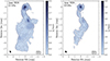 |
Fig. 1. Total intensity images of 3C 84 at 22 and 43 GHz. The total intensity is represented by the contours, using the contour levels at 0.5, 1, 2, 4, 8, 16, 32, and 64% of the peak flux (Smax, 22 GHz = 3.54 Jy/beam, Smax, 43 GHz = 5.94 Jy/beam). The black ellipse in the bottom left corner denotes the common convolving beam with a size of (0.35 × 0.16) mas at a position angle of 18° (uniform weighting), and the black dash in the bottom right corner denotes the projected distance corresponding to 4000 RS for both frequencies. The cut-off is at 4σI for 22 GHz and at 1.5σI for 43 GHz (σI, 22 GHz = 0.93 mJy, σI, 43 GHz = 4.9 mJy). |
3.2. Spectral index distribution
We defined the spectral index α as Sν ∝ ν+α, with Sν being the flux density and ν the observing frequency. In Fig. 2 we present the results of the spectral analysis of 2021, 2022, and 2024, which were generated from total intensity images at 22 and 43 GHz, convolved with the same beam size of (0.35 × 0.16) mas at a position angle of 18°. After the phase self-calibration procedure of VLBI data, the absolute position information is lost, and images at different frequencies need to be aligned manually, which was done using prominent and optically thin parts within the map (Kutkin et al. 2014). We followed the procedure as presented in Paraschos et al. (2021) and performed a 2D cross-correlation on the optically thin part of the 3C 84 jet (Croke & Gabuzda 2008; Nagai et al. 2014; Park et al. 2024), which is marked as the dashed black box in the first epoch in Fig. 2, and applied the shift in right ascension and declination to the lower frequency. For 2021, we found the best alignment of 0.06 mas and −0.02 mas in right ascension and declination, respectively. Our alignment for 2022, with shifts of 0.02 mas in right ascension and 0.0 mas in declination, agrees with the shift reported by Park et al. (2024). For 2024, we found a best alignment in right ascension and declination of 0.06 mas and −0.06 mas, respectively. To evaluate the robustness of the alignment, we varied the sizes and positions for the alignment region and tested changes in alignments using a larger circular beam (see Appendix A.1). Our results remained unaffected. We note that each pixel in the spectral index distribution map has an uncertainty of 10%.
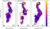 |
Fig. 2. Spectral maps of 3C 84 between 22 and 43 GHz. The total intensity is represented by the contours, using the contour levels at 1, 2, 4, 8, 16, 32, and 64% of the peak flux at 22 GHz, with a cut-off of 8σI for all epochs. The black ellipse in the bottom left corner denotes the convolving circular beam size of (0.35 × 0.16) mas at a position angle of 18° for all epochs, and the black dash in the bottom right corner denotes the projected distance corresponding to 4000 RS and 0.37 pc. The dashed box indicates the optically thin jet region that was used for the cross-correlation calculations as described in Sect. 3.2. The black arrow marks the knot deflection point, as mentioned in Sect. 3.2. |
In all three epochs, we observe an inverted and flat spectrum in the core region of 3C 84. Following the jet downstream, the spectral index gradually decreases, which was also observed in previous studies (Paraschos et al. 2021, 2022b; Park et al. 2024). In 2021 and 2022, the eastern edge of the first ∼0.5 mas of the inner jet region (region R1 and the region marked with an arrow in Fig. 2) downstream of the jet is flat and inverted. Park et al. (2024) denoted this region in 2022 as the knot deflection point. It coincides with the region in which a jet component changes its direction drastically (for more information see Park et al. 2024). Furthermore, in the first two epochs within the first ∼1.5 mas downstream from the core, we observe flattened spectra that extend as two limbs along the jet direction (regions R2 in Fig. 2). This morphology corresponds to a limb-brightened spectral index distribution, where the jet limbs exhibit flatter or inverted spectra, while the spectrum towards the confined jet edges is steeper. In 2024, the spectral index in the core region of 3C 84 is flat, while the downstream jet in 2024 is steep and shows an inverted spectrum only in the east limb in the innermost jet or parsec-scale region. To evaluate the spectral index evolution in the region of the limbs, we determined the spectral indices along slices at ∼1.2 mas and along parallel-shifted slices at ∼1.0 mas and ∼1.4 mas jet downstream, which are indicated by the dashed black lines in Fig. A.2. In the first two epochs, the limb structure is evident in the inset plot, while it is absent for the west limb in the last epoch. Therefore, we conclude that the above-mentioned limb structure observed in 2021 and 2022 is less pronounced in 2024.
3.3. Light-curve information
We used the γ-ray light curve of 3C 84 in order to investigate whether morphological and spectral changes were associated with the emission of high-energy photons. In Fig. 3 we present the radio and γ-ray light curves of 3C 84 employing publicly available data by SMA and Fermi-LAT between 2019 and 2025. Between 2019 and mid 2022, the radio and γ-ray light curves show no signs of flaring events. After 2023, the flux density in the radio regime starts to increase by a factor of ∼1.5 until the end of the available data. For the Fermi-LAT data, however, we observe a flare starting in June 2022, until it reached its maximum in March 2023 with a peak of (0.83 ± 0.03)×10−6 ph cm−2 s−1, after which the photon flux decreases. A more detailed examination of the relation of this high-energy variability to the filamentary structure and spectral index changes in the jet is given in Sect. 4.
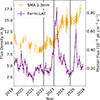 |
Fig. 3. Light curves of 3C 84between 2019 and 2025. The orange curve denotes data by SMA at 1.3 mm, the purple curve denotes monthly binned Fermi-LAT data, and the grey shaded vertical lines show the epochs of available observational VLBI data at 22 and 43 GHz. |
3.4. Magnetic field strength
To estimate the magnetic field strength, we assumed a conical jet with an optically thin spectral index α0 and equipartition between the radiating particle and the magnetic field, leading to a core shift factor of kr = 1 (Lobanov 1998; Hirotani 2005; Ricci et al. 2022). We calculated the core-position offset measure as in Hirotani (2005),
![Mathematical equation: $$ \begin{aligned} \Omega _{\rm r\nu } = 4.85 \times 10^{-9} \, \frac{\Delta r_{\mathrm{mas}} \, D_{\rm L}}{(1+z)^2} \left(\frac{\nu _1^{1/k_{\rm r}} \, \nu _2^{1/k_{\rm r}}}{\nu _2^{1/k_{\rm r}} - \nu _1^{1/k_{\rm r}}}\right) \quad \mathrm{[pc\,GHz]}, \end{aligned} $$](/articles/aa/full_html/2026/05/aa58540-25/aa58540-25-eq1.gif) (1)
(1)
with Δrmas being the core shift between frequency ν1 and ν2 in mas (ν1 < ν2), and DL is the luminosity distance in parsec. We found core-position offset measures of  pc GHz,
  pc GHz, and
  pc GHz. Further, we calculated the magnetic field in the core region of 3C 84 following Fromm et al. (2013),
![Mathematical equation: $$ \begin{aligned} B_0 \approx &\frac{2 \pi m_{\rm e}^2 c^4}{e^3} \left[\frac{e^2}{m_{\rm e} c^3} \left(\frac{\Omega _{\rm r\nu }}{r_0 \sin \theta }\right)^{k_{\rm r}}\right]^{\frac{5 - 2\alpha _0}{7 - 2\alpha _0}} \Biggl [\pi C(\alpha _0) \frac{r_0 m_{\rm e} c^2}{e^2} \frac{-2\alpha _0}{\gamma _{\min }^{2\alpha _0 + 1}}\\&\times \frac{\phi }{\sin \theta }K(\gamma , \alpha _0) \left(\frac{\delta }{1+z}\right)^{\frac{3}{2} - \alpha _0}\Biggr ]^{\frac{-2}{7-2\alpha _0}}\quad \mathrm{[G]},\nonumber \end{aligned} $$](/articles/aa/full_html/2026/05/aa58540-25/aa58540-25-eq5.gif) (2)
(2)
in which
 (3)
(3)
The coefficient C(α0) is tabulated in Hirotani (2005), r0 is the distance from the VLBI core to the jet apex and corresponds to the core shift (r02021 = 0.14 ± 0.01 mas, r02022 = 0.02 ± 0.001 mas, r02024 = 0.08 ± 0.01 mas), γmax and γmin are the maximum and minimum Lorentz factor, ϕ is the half-opening angle, θ is the jet viewing angle, and δ = [Γ(1 − β cos θ)]−1 is the Doppler factor. We adapted the parameters reported by Paraschos et al. (2021)δ ∼ 1.18 − 1.25, θ ∼ 20° −65°, ϕ ∼ 2.8° −20°, and γmax = 103 − 105 (Abdo et al. 2009) and γmin = 1. For the limit α0 → −0.5, the right-hand side of K(γ, α0) in Eq. (3) converges to 1/ln[γmax/γmin] (Hirotani 2005). Finally, the magnetic field in 2021 is B02021 ≈ (30.6 − 75.8) G, in 2022 B02022 ≈ (50.2 − 124.2) G, and in 2024 B02024 ≈ (35.0 − 86.6) G.
Furthermore, we calculated the magnetic field strength in the region of the filaments at ∼1.2 mas (corresponding to 0.44 pc) downstream from the core. At this distance, the jet remains optically thick, meaning that the relation above is still valid. We applied
 (4)
(4)
where r1.2 mas is the distance of ∼1.2 mas from the core, and b = 1. For 2021, we computed  G, in 2022
  G, and in 2024
  G. We found that the magnetic field strength in the core region and the limbs is consistent within their ranges over three years.
4. Discussion
The multi-epoch VLBI observations presented here reveal novel morphological and spectral details of the temporal evolution of limb-brightened jet structures close to the core of 3C 84 over three years, providing new constraints of its launching and collimation processes. We found a prominent inverted spectrum in the core region in 2021 and 2022, with a gradual steepening farther downstream the jet. In these epochs, the inverted spectrum at the east edge of the inner jet region coincides with the knot deflection point, suggesting free-free absorption due to a dense cold ambient medium (for a detailed description see Kino et al. 2021; Park et al. 2024). We detected a limb-brightened morphology within the first ∼1.5 mas jet downstream, which is also imprinted on the spectral index distribution as flattened spectra in 2021 and 2022 (R2 in Fig. 2). Another bright radio galaxy with a similar limb-brightened geometry is M 87, where intertwined helical threads align with a flattened spectral index (Nikonov et al. 2023). This might be caused by K-H instabilities (Lobanov et al. 2003; Hardee 2003). The observed flattened spectra in region R2 and R3 in Fig. 2 coincide with the areas of possible overlapping filaments, as seen in Paraschos & Mpisketzis (2025), who observed brightness enhancements at ∼1 mas and ∼3 mas from the core. These overlaps are a plausible explanation for the observed morphology. They further suggested that the jet shows an increased emissivity in R3, which might be due to the local decrease in the separation of the two filaments. This is an alternative approach to the overlapping filaments.
In 2024, however, the west limb of the double rail structure in the downstream jet was less pronounced (see Fig. A.2). A possible explanation for this behaviour is the rotation of filaments in the innermost jet region, as discussed in Paraschos & Mpisketzis (2025) and as seen in the animated sequence by Park et al. (2024). In 2021 and 2022, these filaments might have overlapped, inducing a brightness enhancement in the regions in which these filaments cross, which was then imprinted on the spectral index distribution as flattened spectra. In 2023, however, these overlapping filaments might have been the cause of a γ-ray flare, as shown in Fig. 3. Based on the analysis presented in Hodgson et al. (2021; and references therein), this behaviour can be interpreted within a turbulence-induced magnetic reconnection scenario, in which filamentary magnetic structures produced behind a travelling shock front interact and reconnect. As the disturbance (R3) propagates downstream, the increasing turbulence is amplified and disturbs the magnetic field as filaments. This in turn enhances the probability of reconnection events and the formation of mini-jets (e.g. Giannios et al. 2009; Shukla & Mannheim 2020). Such reconnection events can efficiently accelerate particles and produce high-energy emission on sub-parsec scales, potentially within the limb region of the jet (Hodgson et al. 2021; Giannios 2013). We therefore suggest that the γ-rays may be produced in the limbs spanning from the core to ∼2 mas downstream. As these filaments continue to rotate, the positions of the overlap shift and might not induce brightness enhancements in the latest epoch. In addition, synchrotron cooling can lead to a steepening of the spectrum downstream from the core (Nikonov et al. 2023).
The observed limb-brightening in the spectral index distribution across all epochs suggests a transverse stratification of the inner jet, consistent with a magnetically dominated flow close to the central engine. General relativistic magnetohydrodynamic (GRMHD) simulations show that this morphology is consistent with a fast-spinning black hole with magnetic field lines reaching the central engine (Takahashi et al. 2018). Moreover, the observed geometry can be associated with a magnetically arrested disc (MAD) and advection-dominated accretion flows (ADAFs; see Narayan & Yi 1995) in which spin energy is extracted from the central engine, favouring a Blandford–Znajek launching process (see Tchekhovskoy et al. 2011; Paraschos et al. 2024b, for more details). We note the limitations of this model. A standard and normal evolution (SANE) model can produce similar geometries, such as a toroidal magnetic field configuration, but the limb-brightened structure is most prominent in simulations for the MAD model (Fromm et al. 2022).
Recent general relativistic magnetohydrodynamic simulations in the parsec scale jet of M 87 showed that a fast-spinning black hole in a MAD state agrees well with the observed jet morphology (Yang et al. 2024). Similarly, this provides further support of the interpretation that the 3C 84 jet is also powered by the Blandford–Znajek mechanism. Further, we find that the magnetic field strengths overlap within their ranges over three epochs and show no high variability within three years.
Previous studies of the magnetic field strength of the jet apex in 3C 84 by Paraschos et al. (2021), Paraschos et al. (2022b) reported lower values than the estimates we presented. They differ by up to an order of magnitude, whereas the estimate by Kim et al. (2019) is of the same order of magnitude as our results. However, Nagai et al. (2017) estimated the magnetic field strength at the jet base of 3C 84 by applying a first-order approximation of a radial magnetic field configuration (B(r)∝r−2), leading to ∼104 G. Similar estimates were reported by O’Sullivan & Gabuzda (2009), who analysed multiple BL-Lac objects, leading to magnetic field strength estimates of ∼104 − 105 G. Furthermore, Kino et al. (2015) reported a magnetic field strength of 50 − 124 G at the jet base of M 87, which is similar to the computed values we presented. The magnetic field strength variability across different studies can be explained by the fact that these estimates are sensitive to model parameters (i.e. r0 and Ωrν) and to the method used to determine the field strength. They can therefore vary across multiple epochs.
Although we adopted a conical jet to calculate the magnetic field strength, we wish to emphasise the limitations of this model. The Stokes I maps in Fig. 1 indicate that on sub-parsec scales, the jet appears more confined and exhibits a morphology closer to a cylindrical shape than to a cone, but expands to a wider conical jet farther downstream (Nagai et al. 2014; Giovannini et al. 2018; Foschi et al. 2025). In addition to the conical jet model, Oh et al. (2022) also tested a parabolical jet model to estimate the black hole location in 3C 84 and concluded that the available data prevented them from reliably distinguishing between the two models. Moreover, the jet geometry cannot be uniquely determined from a qualitative evaluation of Stokes I images alone, as projection effects, Doppler boosting, and transverse stratification can produce similar apparent morphologies. Given the different assumptions adopted in these studies and the uncertainties associated with the observational determination of the models, it is therefore not yet possible to draw a strong conclusion on the most probable jet geometry on sub-parsec scales in 3C 84. We thus adopted the conical jet model as the most physically consistent model and commonly used framework for 3C 84 and to enable direct comparison with previous VLBI studies of AGN jets (Blandford & Königl 1979; Oh et al. 2022; Paraschos et al. 2022b).
5. Conclusions
We presented a detailed analysis of the innermost jet structure of 3C 84 using multi-frequency, multi-epoch VLBI observations at 22 and 43 GHz. Our results provide new constraints on the spectral index properties of the jet, with particular attention to the limb-brightened features near the core region. Our results are summarised below.
-
The spectral index distribution changed significantly over three epochs: in 2021 and 2022, the core region showed inverted spectra with limb-brightened flattened spectral structures in the first few milliarcseconds downstream of the jet; in 2024, the core spectrum was inverted, the region up to ∼1.5 mas jet downstream exhibited a steeper spectral index, and the west limb of the previously observed limb-brightened structure was significantly weaker.
-
We detected persistent limb-brightening in the sub-parsec region across all epochs, suggesting that the observed geometry was produced by a fast-spinning black hole in a MAD or ADAF state, favouring a Blandford–Znajek jet-launching scenario.
-
The limb-brightened and flat spectra in 2021 and 2022 can be explained by overlapping filaments; the non-detection of the west limb in 2024 might be linked to the rotational motion of these filaments, synchrotron cooling after a γ-ray flare, or changes in the interactions of the jet with the ambient medium.
-
The correlation between the spectral evolution, filament rotation, and the γ-ray light curve supports a scenario in which the high-energy emission originates from the limbs.
-
We measured the core shifts leading to magnetic field strengths in the range of (0.8−9.1) G in the region of the limbs.
These results show that the inner jet of 3C 84 is a highly dynamic structure in which the spectral properties, morphology, and magnetic field strength vary on timescales of a few years, likely modulated by filamentary variations and interactions between the jet and the ambient medium.
Data availability
A copy of the reduced images is available at the CDS via https://cdsarc.cds.unistra.fr/viz-bin/cat/J/A+A/709/A192
Acknowledgments
We would like to thank the anonymous referee for their constructive comments, which improved our work. We thank I. Liodakis for valuable comments and insightful discussions. We would like to thank J. Park for providing the data of 2022 and for helpful information and comments on our study. The research leading to these results has received funding from the European Union’s Horizon 2020 research and innovation program under grant agreement No 101004719 [Opticon RadioNet Pilot ORP]. The European VLBI Network is a joint facility of independent European, African, Asian, and North American radio astronomy institutes. Scientific results from data presented in this publication are derived from the following EVN project code: GP058, GP061. This study makes use of VLBA data from the VLBA-BU Blazar Monitoring Program (BEAM-ME and VLBA-BU-BLAZAR; http://www.bu.edu/blazars/BEAM-ME.html), funded by NASA through the Fermi Guest Investigator Program. J. A. H. acknowledges the support of the National Research Foundation of Korea (NRF) (NRF-2021R1C1C1009973) and that this work was supported by the National Research Foundation of Korea (NRF) grant funded by the Korea government (MSIT) RS-2025-16302968. M. M. L. was supported by the FONDECYT Iniciacón grant 11251078. J. Y. K. is supported for this research by the National Research Foundation of Korea (NRF) grant funded by the Korean government (Ministry of Science and ICT; grant no. 2022R1C1C1005255, RS-2022-NR071771) and by the Korea Astronomy and Space Science Institute under the R&D program (Project No. 2025-9-844-00) supervised by the Korea AeroSpace Administration. The Submillimeter Array is a joint project between the Smithsonian Astrophysical Observatory and the Academia Sinica Institute of Astronomy and Astrophysics and is funded by the Smithsonian Institution and the Academia Sinica. We recognize that Maunakea is a culturally important site for the indigenous Hawaiian people; we are privileged to study the cosmos from its summit. This research is based in part on observations obtained with the 100-m telescope of the MPIfR at Effelsberg, observations carried out at the IRAM 30-m telescope operated by IRAM, which is supported by INSU/CNRS (France), MPG (Germany) and IGN (Spain), observations obtained with the Yebes 40-m radio telescope at the Yebes Observatory, which is operated by the Spanish Geographic Institute (IGN, Ministerio de Transportes, Movilidad y Agenda Urbana), and observations supported by the Green Bank Observatory, which is a main facility funded by the NSF operated by the Associated Universities. We acknowledge support from the Onsala Space Observatory national infrastructure for providing facilities and observational support. The Onsala Space Observatory receives funding from the Swedish Research Council through grant no. 2017-00648. This publication makes use of data obtained at the Metsähovi Radio Observatory, operated by Aalto University. This publication acknowledges project M2FINDERS, which is funded by the European Research Council (ERC) under the European Union’s Horizon 2020 research and innovation programme (grant agreement no. 101018682).
References
- Abdo, A. A., Ackermann, M., Ajello, M., et al. 2009, ApJ, 699, 31 [Google Scholar]
- Abdollahi, S., Ajello, M., Baldini, L., et al. 2023, ApJS, 265, 31 [NASA ADS] [CrossRef] [Google Scholar]
- Atwood, W. B., Abdo, A. A., Ackermann, M., et al. 2009, ApJ, 697, 1071 [CrossRef] [Google Scholar]
- Blandford, R. D., & Königl, A. 1979, ApJ, 232, 34 [Google Scholar]
- Blandford, R. D., & Payne, D. G. 1982, MNRAS, 199, 883 [CrossRef] [Google Scholar]
- Blandford, R. D., & Znajek, R. L. 1977, MNRAS, 179, 433 [NASA ADS] [CrossRef] [Google Scholar]
- Blandford, R., Meier, D., & Readhead, A. 2019, ARA&A, 57, 467 [NASA ADS] [CrossRef] [Google Scholar]
- Boccardi, B., Perucho, M., Casadio, C., et al. 2021, A&A, 647, A67 [NASA ADS] [CrossRef] [EDP Sciences] [Google Scholar]
- Croke, S. M., & Gabuzda, D. C. 2008, MNRAS, 386, 619 [CrossRef] [Google Scholar]
- Event Horizon Telescope Collaboration (Akiyama, K., et al.) 2019, ApJ, 875, L3 [Google Scholar]
- Foschi, M., Gómez, J. L., Fuentes, A., et al. 2025, A&A, 696, A17 [NASA ADS] [CrossRef] [EDP Sciences] [Google Scholar]
- Fromm, C. M., Ros, E., Perucho, M., et al. 2013, A&A, 557, A105 [NASA ADS] [CrossRef] [EDP Sciences] [Google Scholar]
- Fromm, C. M., Cruz-Osorio, A., Mizuno, Y., et al. 2022, A&A, 660, A107 [NASA ADS] [CrossRef] [EDP Sciences] [Google Scholar]
- Fuentes, A., Gómez, J. L., Martí, J. M., et al. 2023, Nat. Astron., 7, 1359 [NASA ADS] [CrossRef] [Google Scholar]
- Giannios, D. 2013, MNRAS, 431, 355 [NASA ADS] [CrossRef] [Google Scholar]
- Giannios, D., Uzdensky, D. A., & Begelman, M. C. 2009, MNRAS, 395, L29 [NASA ADS] [CrossRef] [Google Scholar]
- Giovannini, G., Savolainen, T., Orienti, M., et al. 2018, Nat. Astron., 2, 472 [Google Scholar]
- Gurwell, M. A., Peck, A. B., Hostler, S. R., Darrah, M. R., & Katz, C. A. 2007, ASP Conf. Ser., 375, 234 [NASA ADS] [Google Scholar]
- Hardee, P. E. 2003, ApJ, 597, 798 [NASA ADS] [CrossRef] [Google Scholar]
- Hirotani, K. 2005, ApJ, 619, 73 [Google Scholar]
- Ho, P. T. P., Moran, J. M., & Lo, K. Y. 2004, ApJ, 616, L1 [Google Scholar]
- Hodgson, J. A., Rani, B., Oh, J., et al. 2021, ApJ, 914, 43 [NASA ADS] [CrossRef] [Google Scholar]
- Högbom, J. A. 1974, A&AS, 15, 417 [Google Scholar]
- Janssen, M., Goddi, C., van Bemmel, I. M., et al. 2019, A&A, 626, A75 [NASA ADS] [CrossRef] [EDP Sciences] [Google Scholar]
- Kam, M., Hodgson, J. A., Park, J., et al. 2024, ApJ, 970, 176 [NASA ADS] [Google Scholar]
- Kim, J.-Y., Krichbaum, T. P., Marscher, A. P., et al. 2019, A&A, 622, A196 [NASA ADS] [CrossRef] [EDP Sciences] [Google Scholar]
- Kim, D.-W., Janssen, M., Krichbaum, T. P., et al. 2023, A&A, 680, L3 [NASA ADS] [CrossRef] [EDP Sciences] [Google Scholar]
- Kino, M., Takahara, F., Hada, K., et al. 2015, ApJ, 803, 30 [NASA ADS] [CrossRef] [Google Scholar]
- Kino, M., Niinuma, K., Kawakatu, N., et al. 2021, ApJ, 920, L24 [CrossRef] [Google Scholar]
- Kutkin, A. M., Sokolovsky, K. V., Lisakov, M. M., et al. 2014, MNRAS, 437, 3396 [Google Scholar]
- Lobanov, A. P. 1998, A&A, 330, 79 [NASA ADS] [Google Scholar]
- Lobanov, A., Hardee, P., & Eilek, J. 2003, New Astron. Rev., 47, 629 [CrossRef] [Google Scholar]
- Lu, R.-S., Asada, K., Krichbaum, T. P., et al. 2023, Nature, 616, 686 [CrossRef] [Google Scholar]
- Nagai, H., Orienti, M., Kino, M., et al. 2012, MNRAS, 423, L122 [Google Scholar]
- Nagai, H., Haga, T., Giovannini, G., et al. 2014, ApJ, 785, 53 [Google Scholar]
- Nagai, H., Fujita, Y., Nakamura, M., et al. 2017, ApJ, 849, 52 [NASA ADS] [CrossRef] [Google Scholar]
- Narayan, R., & Yi, I. 1995, ApJ, 452, 710 [NASA ADS] [CrossRef] [Google Scholar]
- Nikonov, A. S., Kovalev, Y. Y., Kravchenko, E. V., Pashchenko, I. N., & Lobanov, A. P. 2023, MNRAS, 526, 5949 [NASA ADS] [CrossRef] [Google Scholar]
- Oh, J., Hodgson, J. A., Trippe, S., et al. 2022, MNRAS, 509, 1024 [Google Scholar]
- O’Sullivan, S. P., & Gabuzda, D. C. 2009, MNRAS, 400, 26 [Google Scholar]
- Paraschos, G. F., & Mpisketzis, V. 2025, A&A, 696, L7 [NASA ADS] [CrossRef] [EDP Sciences] [Google Scholar]
- Paraschos, G. F., Kim, J. Y., Krichbaum, T. P., & Zensus, J. A. 2021, A&A, 650, L18 [NASA ADS] [CrossRef] [EDP Sciences] [Google Scholar]
- Paraschos, G., Kim, J. Y., Krichbaum, T., et al. 2022a, European VLBI Network Mini-Symposium and Users’ Meeting 2021, 2021, 43 [Google Scholar]
- Paraschos, G. F., Krichbaum, T. P., Kim, J. Y., et al. 2022b, A&A, 665, A1 [NASA ADS] [CrossRef] [EDP Sciences] [Google Scholar]
- Paraschos, G. F., Mpisketzis, V., Kim, J.-Y., et al. 2023, A&A, 669, A32 [NASA ADS] [CrossRef] [EDP Sciences] [Google Scholar]
- Paraschos, G. F., Debbrecht, L. C., Kramer, J. A., et al. 2024a, A&A, 686, L5 [NASA ADS] [CrossRef] [EDP Sciences] [Google Scholar]
- Paraschos, G. F., Kim, J. Y., Wielgus, M., et al. 2024b, A&A, 682, L3 [NASA ADS] [CrossRef] [EDP Sciences] [Google Scholar]
- Park, J., Kino, M., Nagai, H., et al. 2024, A&A, 685, A115 [NASA ADS] [CrossRef] [EDP Sciences] [Google Scholar]
- Planck Collaboration XIII. 2016, A&A, 594, A13 [NASA ADS] [CrossRef] [EDP Sciences] [Google Scholar]
- Punsly, B., Nagai, H., Savolainen, T., & Orienti, M. 2021, ApJ, 911, 19 [Google Scholar]
- Ricci, L., Boccardi, B., Nokhrina, E., et al. 2022, A&A, 664, A166 [NASA ADS] [CrossRef] [EDP Sciences] [Google Scholar]
- Shepherd, M. C. 1997, ASP Conf. Ser., 125, 77 [Google Scholar]
- Shukla, A., & Mannheim, K. 2020, Nat. Commun., 11, 4176 [NASA ADS] [CrossRef] [Google Scholar]
- Strauss, M. A., Huchra, J. P., Davis, M., et al. 1992, ApJS, 83, 29 [Google Scholar]
- Takahashi, K., Toma, K., Kino, M., Nakamura, M., & Hada, K. 2018, ApJ, 868, 82 [NASA ADS] [CrossRef] [Google Scholar]
- Tchekhovskoy, A., Narayan, R., & McKinney, J. C. 2011, MNRAS, 418, L79 [NASA ADS] [CrossRef] [Google Scholar]
- Walker, R. C., Dhawan, V., Romney, J. D., Kellermann, K. I., & Vermeulen, R. C. 2000, ApJ, 530, 233 [Google Scholar]
- Walker, R. C., Hardee, P. E., Davies, F. B., Ly, C., & Junor, W. 2018, ApJ, 855, 128 [Google Scholar]
- Weaver, Z. R., Jorstad, S. G., Marscher, A. P., et al. 2022, ApJS, 260, 12 [NASA ADS] [CrossRef] [Google Scholar]
- Yang, H., Yuan, F., Li, H., et al. 2024, Sci. Adv., 10, eadn3544 [NASA ADS] [CrossRef] [Google Scholar]
Comparative tests demonstrate that rPICARD produces improved data calibration results than the calibration procedure performed with AIPS, as shown in Kim et al. (2023).
Appendix A: Additional information
Figure A.1 presents the same images as in Fig. 2 but with a circular convolving beam of 0.25 mas and Fig. A.2 shows the spectral index distribution along slices at ∼1.2 mas, and along parallel-shifted slices at ∼1.0 mas and ∼1.4 mas jet downstream. The discussion of these map are covered in the main text.
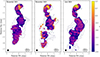 |
Fig. A.1. Spectral maps of 3C 84 between 22 and 43 GHz. The total intensity is represented by the contours, using the contour levels at 1, 2, 4, 8, 16, 32, and 64% of the peak flux at 22 GHz, with a cut-off of 8σI for all epochs. The black circle in the bottom left corner denotes the convolving, circular beam size of 0.25 mas for all epochs and the black dash in the bottom right corner denotes the projected distance corresponding to 4000 RS and 0.37 pc. |
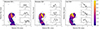 |
Fig. A.2. Similar to Fig. 2, but the insets show the spectral indices distributions along slices at ∼1.2 mas, and along parallel-shifted slices at ∼1.0 mas and ∼1.4 mas jet downstream, as indicated by the black dashed lines. The grey shaded area around the inset plot indicates the 10% uncertainty of the spectral index. |
All Tables
All Figures
|
Fig. 1. Total intensity images of 3C 84 at 22 and 43 GHz. The total intensity is represented by the contours, using the contour levels at 0.5, 1, 2, 4, 8, 16, 32, and 64% of the peak flux (Smax, 22 GHz = 3.54 Jy/beam, Smax, 43 GHz = 5.94 Jy/beam). The black ellipse in the bottom left corner denotes the common convolving beam with a size of (0.35 × 0.16) mas at a position angle of 18° (uniform weighting), and the black dash in the bottom right corner denotes the projected distance corresponding to 4000 RS for both frequencies. The cut-off is at 4σI for 22 GHz and at 1.5σI for 43 GHz (σI, 22 GHz = 0.93 mJy, σI, 43 GHz = 4.9 mJy). |
| In the text | |
|
Fig. 2. Spectral maps of 3C 84 between 22 and 43 GHz. The total intensity is represented by the contours, using the contour levels at 1, 2, 4, 8, 16, 32, and 64% of the peak flux at 22 GHz, with a cut-off of 8σI for all epochs. The black ellipse in the bottom left corner denotes the convolving circular beam size of (0.35 × 0.16) mas at a position angle of 18° for all epochs, and the black dash in the bottom right corner denotes the projected distance corresponding to 4000 RS and 0.37 pc. The dashed box indicates the optically thin jet region that was used for the cross-correlation calculations as described in Sect. 3.2. The black arrow marks the knot deflection point, as mentioned in Sect. 3.2. |
| In the text | |
|
Fig. 3. Light curves of 3C 84between 2019 and 2025. The orange curve denotes data by SMA at 1.3 mm, the purple curve denotes monthly binned Fermi-LAT data, and the grey shaded vertical lines show the epochs of available observational VLBI data at 22 and 43 GHz. |
| In the text | |
|
Fig. A.1. Spectral maps of 3C 84 between 22 and 43 GHz. The total intensity is represented by the contours, using the contour levels at 1, 2, 4, 8, 16, 32, and 64% of the peak flux at 22 GHz, with a cut-off of 8σI for all epochs. The black circle in the bottom left corner denotes the convolving, circular beam size of 0.25 mas for all epochs and the black dash in the bottom right corner denotes the projected distance corresponding to 4000 RS and 0.37 pc. |
| In the text | |
|
Fig. A.2. Similar to Fig. 2, but the insets show the spectral indices distributions along slices at ∼1.2 mas, and along parallel-shifted slices at ∼1.0 mas and ∼1.4 mas jet downstream, as indicated by the black dashed lines. The grey shaded area around the inset plot indicates the 10% uncertainty of the spectral index. |
| In the text | |
Current usage metrics show cumulative count of Article Views (full-text article views including HTML views, PDF and ePub downloads, according to the available data) and Abstracts Views on Vision4Press platform.
Data correspond to usage on the plateform after 2015. The current usage metrics is available 48-96 hours after online publication and is updated daily on week days.
Initial download of the metrics may take a while.