| Issue |
A&A
Volume 696, April 2025
|
|
|---|---|---|
| Article Number | L7 | |
| Number of page(s) | 6 | |
| Section | Letters to the Editor | |
| DOI | https://doi.org/10.1051/0004-6361/202554201 | |
| Published online | 08 April 2025 | |
Letter to the Editor
Unravelling the dynamics of cosmic vortices: Probing a Kelvin-Helmholtz instability in the jet of 3C 84
1
Max-Planck-Institut für Radioastronomie, Auf dem Hügel 69, D-53121 Bonn, Germany
2
Department of Physics, National and Kapodistrian University of Athens, Panepistimiopolis, 15783 Zografos, Greece
3
Institut für Theoretische Physik, Goethe Universität Frankfurt, Max-von-Laue-Str.1, 60438 Frankfurt am Main, Germany
⋆ Corresponding author; This email address is being protected from spambots. You need JavaScript enabled to view it.
Received:
20
February
2025
Accepted:
18
March
2025
Abstract
Understanding the creation of relativistic jets originating from active galactic nuclei (AGNs) requires a thorough understanding of the accompanying plasma instabilities. Our high-sensitivity, high-resolution, global, very-long-baseline-interferometry observations of the jet in the radio galaxy 3C 84 have enabled us to study its inner morphology. We find that its thread-like pattern can be described by a Kelvin-Helmholtz instability, consisting of four instability modes. Our model favours a jet described by a Mach number of Mj = 5.0 ± 1.7 and a sound speed of αj = 0.14 ± 0.06. On this basis, we are able to describe the internal structure of 3C 84 and tentatively connect the origin of the instability to disc accretion activity.
Key words: techniques: high angular resolution / techniques: interferometric / galaxies: active / galaxies: jets / galaxies: individual: 3C 84 (NGC 1275)
© The Authors 2025
 Open Access article, published by EDP Sciences, under the terms of the Creative Commons Attribution License (https://creativecommons.org/licenses/by/4.0), which permits unrestricted use, distribution, and reproduction in any medium, provided the original work is properly cited.
This article is published in open access under the Subscribe to Open model.
Open Access funding provided by Max Planck Society.
1. Introduction
With the increasing sensitivity of modern very-long-baseline-interferometry (VLBI) arrays, a growing number of active galactic nucleus (AGN) jets have been shown to exhibit filamentary structures. Such structures have been mostly identified in parsec-scale (pc-scale) jets (e.g. Lobanov & Zensus 2001; Hardee 2003; Perucho et al. 2012; Vega-García et al. 2019; Fuentes et al. 2023; Traianou et al. 2024; Britzen et al. 2024). One exception is the jet of M 87, where sub-pc-scale structures have been identified (e.g. Lobanov et al. 2003; Hardee & Eilek 2011; Pasetto et al. 2021; Nikonov et al. 2023). A persistent characteristic of these sources is that they exhibit edge brightening, whereby the outer sheath of the jet is brighter than the inner spine.
The radio galaxy NGC 1275, harbouring the radio source 3C 84, is another example where a double rail structure has been identified (e.g. Nagai et al. 2016; Giovannini et al. 2018; Paraschos et al. 2022; Savolainen et al. 2023). It is one of the nearest and brightest radio sources in the northern sky, making it optimally suited to investigations of the characteristics of the plasma that constitutes the jet. Its bifurcated morphology, reaching deep into the core region (e.g. Giovannini et al. 2018; Punsly et al. 2021; Paraschos et al. 2024a), is indicative of instabilities present in the plasma. Furthermore, in the sub-parsec-scale region, different velocities have been observed (e.g. Hodgson et al. 2021; Weaver et al. 2022; Paraschos et al. 2022), suggestive of Kelvin-Helmholtz (K-H) instability propagation. Furthermore, 3C 84 also exhibits variability on the time scales of a few decades (e.g. Hodgson et al. 2018; Paraschos et al. 2023), which might also be connected to the projection effects of twisting filaments.
Such filaments provide a wealth of insights into the physics governing jets. For example, by modelling the K-H instability modes (e.g. Perucho et al. 2005; Mizuno et al. 2007) or by testing current driven instability modes against simulations (CDI; e.g. Mizuno et al. 2009; McKinney & Blandford 2009), we can constrain jet propagation parameters. These include the jet’s internal Mach number, Mj, density ratio of the jet to the ambient medium, η, sound speed of the jet and the ambient medium (αj and αx respectively), and the instability propagation velocity, vw.
In this work, we have leveraged the excellent, sub-parsec-scale resolution achieved when observing 3C 84 with centimetre VLBI, to investigate the jet’s filamentary structure in the vicinity of the central engine in detail. We invoked the K-H instability (see e.g. Hardee 1984, 1986, 1987, 2000; Hardee et al. 1997) to gain analytical results for the underlying modes and to make predictions about the jet’s morphology.
This paper is structured as follows. In Sect. 2, we briefly touch upon the data reduction and discuss our results. In Sect. 3, we examine the modelling parameters of the filamentary structures of 3C 84. Finally, in Sect. 4, we summarise our conclusions. Throughout this work, we assume a Λ cold dark matter cosmology, with H0 = 67.8 kms−1 Mpc−1, ΩΛ = 0.692, and ΩM = 0.308 (Planck Collaboration XIII 2016). At a z = 0.0176 (Strauss et al. 1992), this is equivalent to a megaparsec luminosity distance of DL = 78.9 ± 2.4 Mpc and a parsec-to-milliarcsecond (pc-mas) conversion factor of ψ = 0.36 pc mas−1.
2. Observations, methods, and results
2.1. Observations
The array configuration, data correlation, and calibration, as well as the imaging were previously discussed in Paraschos et al. (2024b). In brief, 3C 84 was observed in November 2021 at 22 GHz by a global VLBI array, consisting mainly of the European VLBI Network (EVN) in conjunction with a number of additional antennas, amounting to a total of 22. The post-processing consisted of calibrating the data with the rPicard (Janssen et al. 2019) and polsolve (Martí-Vidal et al. 2021) pipelines and imaging their output using the CLEAN algorithm within the difmap software package (Shepherd et al. 1994).
While in Paraschos et al. (2024b), the focus of the analysis was on the linearly polarised signal traced by the double-thread structure mainly in the core region (see also Kramer et al. 2024); here, we investigated these threads in the total extent of the downstream jet. The first step to identify them was to convolve the image with a circular beam the size of 0.6 mas, which is approximately double the size of the nominal beam (0.17 × 0.40) mas. This step was required to blur out the finer scale structure, allowing us to robustly determine the jet ridge line1 (see e.g. Paraschos et al. 2022). Next, we fitted slices locally perpendicular to the jet axis with a bimodal function; the slices were performed on the jet image convolved with its nominal beam. The distance between each slice (step size) was 0.1 mas. Our choice of a bimodal function fit was a natural consequence of the apparent double rail morphology present in 3C 84. Finally, we differentiated between the two peaks of the fit by assigning the higher peaked flux density ones to the green thread (‘T1’) and the lower peaked flux density ones to the blue thread (‘T2’). The smoothed threads T1 and T2 are presented in Fig. 1. An alternative thread identification is discussed in Appendix A.
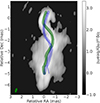 |
Fig. 1. Stokes I image of 3C 84 showcasing a filamentary morphology. The colour scale is logarithmic and the units are mJy/beam. The dark green ellipse in the lower left corner shows the convolving beam size (0.17 × 0.40) mas. Two threads are superimposed: the green (blue) one traces the filament characterised by higher (lower) flux density. Their widths correspond to the position uncertainty. The computed K-H models are shown with the continuous thin lines, matching the colours of the double helix morphology. The dotted line corresponds to a linear fit of the ridge line with the purpose of determining the position angle (PA = 4.5°) of the jet propagation. The image was turned by −4.5° to align the jet axis with the ordinate. A cutoff at ∼5 mas from the jet apex was implemented, to only include high-S/N areas in our fit. |
The two threads showcase an intertwining, helical pattern suggestive of a Kelvin-Helmholtz instability. They are most likely the result of the interplay of the plasma of the jet and the surrounding medium, spurned by an external periodic source, such as jet axis precession, accretion disc rotation, nutation, or jet wobbling (Lobanov & Zensus 2001). Such a periodicity is also identified in relativistic magneto-hydrodynamic simulations (e.g. Mizuno et al. 2015; Fuentes et al. 2018). The threads can be described by the jet internal (external medium) Mach number, Mj (Mx), and velocity, βj (βx). Finally, an auxiliary measurables is the ratio between the internal and external medium density, ηj ≡ ρj/ρx, also called the enthalpy ratio.
2.2. Methods
To fit the two threads, we assumed that they are best approximated by a sum of sinusoidal modes following a helical trajectory, which we then projected on the plane of the sky. Mathematically, this can be expressed as:
 (1)
(1)
and
 (2)
(2)
where A ∝ AiRj(z)ki is the amplitude, λ ∝ λiRj(z)ki is the wavelength, and ki is the longitudinal wavenumber, x is the distance of the jet from the apex, φ is the phase, and θj is the viewing angle to our line of sight to the jet. The amplitude (Ai) and measured wavelength (λi) are both proportional to the jet radius, Rj(x)/pc (Hardee 2000). Additionally, we assumed that jet opening half-angle, ϕj, satisfies the relation  , which ensures that our computed solutions are within linear perturbation in a cylindrical jet regime (e.g. Hardee 1986, 1987).
Determining the appropriate number of modes to fit requires a careful consideration of its impact on the goodness of fit. We chose to fit the first four modes (χ42∼1) and the resulting fits are shown with the thin blue and green lines in Fig. 1. While the green thread fit is confined within the uncertainty band, we observe a deviation of the blue band from the observed threads, particularly in regions farther from the central black hole. This behaviour arises from our model selection criterion. Adding a fifth mode marginally decreased the formal χ2 by fitting these low signal-to-noise (S/N) regions better, but it also increased the Akaike information criterion (AIC) value by a factor of ∼1.3. As a result, this indicates that such an increase in the model’s complexity was not justified. Similarly, employing only three modes did not result in an adequate fit, indicated by the result of χ32 = 3.
For each mode of the fit, we then calculated the corresponding resonant K-H mode wavelength λn, m*, given by
 (3)
(3)
The parameters (n, m), appearing in the above Eq. (3) are the azimuthal wave number and its order, respectively. For relativistic jets, the first three azimuthal numbers are expected to be most influential (e.g. Hardee 2000; Mizuno et al. 2007). They correspond to the pinch (n = 0), helical (n = 1), and elliptical (n = 2) instability, respectively. Their order, on the other hand, controls whether the perturbation is manifested in the surface (m = 0) or body (m > 0) of the jet. We note that since λ* depends only on the physical characteristics of the jet, its value should not differ per mode (see e.g. Lobanov et al. 2003).
Furthermore, when comparing the modelled wavelengths (λnm*) to all the measured ones (λi) in order to identify each mode, we tolerated a discrepancy, ϵλi, of up to 25% between λnm* and λi per mode. This discrepancy was defined as:
![Mathematical equation: $$ \begin{aligned} \epsilon _{\lambda _{\rm i}} \equiv 100\cdot \dfrac{\left\Vert\lambda ^*_{\rm nm}- \lambda _{i}\right\Vert}{\lambda ^*_{\rm nm}}\ [\%]. \end{aligned} $$](/articles/aa/full_html/2025/04/aa54201-25/aa54201-25-eq5.gif) (4)
(4)
Finally, we used a Markov chain Monte Carlo approach to sample the parameters of each mode, estimating their distribution and uncertainties, and selecting the most probable mode (i.e. the peak of the distribution). All the parameters and their respective values of this section are listed in the top panel of Table 1.
Model input (top) and output (bottom) parameters.
2.3. Results
The pc-scale, helical jet structure of 3C 84, consisting of two threads, T1 and T2, is optimally approximated by the combination of four modes: a helical surface (Hs) and body (Hb1) mode and an elliptical surface (Es) and body (Eb1) mode. The resulting fit parameters are shown in Table 2. We find that the surface modes exhibit longer wavelengths than the body modes, in line with theoretical expectations (e.g. Hardee 2013). Their amplitudes also follow the same trend.
K-H modelled parameters for T1 and T2.
Determining the measurables, Mx, Mj, as well as the jet pattern speed, βw, sound speed (αj), and ambient medium sound speed (αx) requires a relation between them and the measured K-H modes. Such a relation exists between the resonant wavelength, λ* (see also Vega-García et al. 2019), and Mx, which is given by:
 (5)
(5)
Here, βw is given by:
 (6)
(6)
where we identified the apparent pattern velocity,  , with that of component ‘C3’ (Nagai et al. 2014). On the other hand, Mj is given by:
 (7)
(7)
and its relativistic counterpart, ℳj ≡ ΓjMj. Finally, the aforementioned sound speeds can then be calculated via the relation:
![Mathematical equation: $$ \begin{aligned} \alpha _{\rm [j,\ x]} = \beta _{\rm j}/M_{\rm [j,\ x]}. \end{aligned} $$](/articles/aa/full_html/2025/04/aa54201-25/aa54201-25-eq10.gif) (8)
(8)
In this framework, the derived jet values based on our instability analysis are listed in the bottom part of Table 1.
3. Discussion
3.1. Modelled jet characteristics
Our analysis in this work presents a self-consistent picture of the internal jet structure. A strong indication in favour of our model is the fact that we found the measured and predicted wavelengths to agree within the error budget. The associated Mj, x values are moderate with Mx > Mj, indicating that the jet’s density is lower than that of its surrounding interstellar medium. This is consistent with the reported internal ( ) and external (
 ) density values for 3C 84. Specifically, Kim et al. (2019) reported a result of
  , whereas a number of estimates exist for
  (e.g. Fujita & Nagai 2017; Nagai et al. 2017; Park et al. 2024). Furthermore, the sound speeds of the internal and external medium are consistent with a light, electron-positron plasma pair (Lobanov & Zensus 2001). Interestingly, a VLBI-independent approach by Paraschos et al. (2023) using variability light curves came to the same conclusion about the 3C 84 jet’s particle composition. The low value of αx points to a sub-relativistic ambient medium. Finally, the two threads also naturally explain the prominent limb brightening of 3C 84 as a manifestation of the K-H instability.
3.2. Brightness enhancements
Numerous jets across different spatial scales are characterised by moving components and the trajectories have been traced for years (e.g. Weaver et al. 2022). Theories have been put forth to explain them; for example, they have been attributed to Doppler boosting due to geometric effects or shocks propagating through the bulk jet flow (see e.g. Liodakis et al. 2020; Paraschos 2025). However, their exact nature remains elusive.
The sub-pc scale jet in 3C 84 is similarly characterised by such emission features in its downstream region. In Fig. 1 we can identify one such brightness enhancement in the south-west of the core, at a distance of ∼2 mas. Interestingly, this area coincides with an overlap of the two threads. As discussed in Nikonov et al. (2023) for the M 87 jet, these crossing K-H threads could also provide a natural explanation for these regions of enhanced emission. The authors also identified a spectral index flattening in the area where the crossing occurs. A spectral index map (22–43 GHz) of 3C 84, characterised by similar resolution to this work, was presented in Park et al. (2024), based on observations taken a year later. Intriguingly, the spectral index appears flatter in that area as well2, while also being brighter than the rest of the approaching jet. In combination with our work, this result provides further evidence that overlapping K-H threads are a plausible mechanism behind the brightness enhancements in jets in the optically thin regime.
3.3. Driving mechanism
Connecting the predicted longest unstable wavelengths, λn, m1, to an external driving mechanism requires knowledge about the mechanism’s driving period. Furthermore, the body modes will be attenuated at the longest unstable wavelength, λn, m1, such that:
 (9)
(9)
Here, λpred; n, m* is the predicted resonant wavelength per K-H mode. On the other hand, body modes are characterised by the absence of such a longest unstable wavelength; thus, they can theoretically have arbitrarily long wavelengths (Lobanov & Zensus 2001). The λpred; n, m* values are shown in Table 3.
Predicted K-H mode resonant and longest unstable wavelengths.
A number of different periodicity values have been identified in 3C 84, based on different measurables, which differ by orders of magnitude. For example, Britzen et al. (2019) identified a periodicity of the order of 40–100 years, based on radio light-curves. Similarly, Dominik et al. (2021) provided a periodicity estimate of up to 30 years, based on the movement of the jet internal position angle. On the other hand, X-ray observations of the same source are suggestive of time scales of the order of tens of millions of years Dunn et al. (2006). Using the predicted λpred; n, m* value from our K-H analysis, we can calculate a combination of the periodicity, Tp, and the longest unstable wavelength, λ1, which satisfies the constraint imposed by Eq. (9). This is achieved by using the relation which links Tp to λ1 (see Lobanov & Zensus 2001) and is given by:
 (10)
(10)
Here, δj is the jet Doppler factor, such that δj ≡ (Γj(1 − βj sin θj))−1. We find that in order to satisfy Eq. (9), a periodicity of Tp = 30 ± 10 years is required, resulting in the predictions for λn, m1 shown in Table 3. Our computed periodicity is more consistent with the first two literature values (see Britzen et al. 2019; Dominik et al. 2021), which are associated with jet precession. Finally, we compared our computed periodicity to the structural changes of the 3C 84 jet, as shown in Kam et al. (2024). Those authors displayed the spatial evolution of the jet structure over a 12 year time span, which roughly equals half of Tp. Based on our prediction, we would expect that the sinusoidal nature of the overall jet structure, imposed by the helical surface mode, has shifted the jet direction by half a wavelength. Intriguingly, this behaviour is exactly mirrored in images published in the work of Kam et al. (2024). The inner jet starts out in 2010 moving in south-eastwardly direction and begins moving south-westwards by 2022. Consequently, we predict that after another ∼Tp/2, the inner jet will again be directed in the south-eastwardly direction.
Furthermore, we contrast our result to the analysis of the blazar 3C 345, presented in Lobanov & Roland (2005). These authors calculated the characteristic time scales for accretion disc activity in a binary system, such as thermal processes in the accretion disc (∼10 years), the rotational (∼200 years) and precession (∼2500 years) period of the accretion disc, and the orbital (∼500 years) period. Their estimation of that source’s black hole mass (M•3C 345 ∼ 1.4 × 10⁹ M⊙) is similar to that of the 3C 84 system (M•3C 84 ∼ 2 × 10⁹ M⊙; Giovannini et al. 2018), allowing for a direct comparison. In this case, our estimate for Tp is more aligned with the effects attributed to the disc’s activity.
4. Conclusions
In this work, we present an exploration of jet morphology of 3C 84 via K-H instability modelling. Our analysis can be summarised as follows:
-
We modelled the sub-pc jet structure of 3C 84 by fitting a bimodal function to slices drawn transversely to the bulk jet flow.
-
By categorising each of the two modelled peaks based on their respective amplitudes, we were able to retrieve an intertwining, helical morphology.
-
We found that a Kelvin-Helmholtz instability can adequately describe this morphology; the corresponding Mach numbers and sound speeds for the internal (external) medium are Mj = 5.0 ± 1.7, αj = 0.14 ± 0.06 (Mx = 9.8 ± 3.2, αx = 0.07 ± 0.02).
-
These values are indicative of a low-density electron-positron pair plasma flow, surrounded by a sub-relativistic ambient medium.
-
The timescales associated with these values favour the assumption that the underlying periodic driving mechanism is connected to processes related to disc accretion.
In summary, we have shown that high-sensitivity, high-fidelity images of nearby jetted-AGNs can be utilised to explore the interplay between outflows and instabilities. Future facilities, such as the next generation Very Large Array and the Square Kilometre Array, will offer even more advancements in sensitivity and enable us to increase the number of jets to further improve such analyses.
Here, we define the ridge line as the main jet axis.
We note, however, that in Paraschos et al. (2021) the spectral index appears more homogeneous in that area, which can be explained by source variability over longer timescales.
Acknowledgments
We would like to thank the anonymous referee for the beneficial comments. We would also like to thank I. Liodakis, A. Lobanov, A. Nikonov, and T. Savolainen for the fruitful discussions, which improved this manuscript greatly. This research is supported by the European Research Council advanced grant “M2FINDERS - Mapping Magnetic Fields with INterferometry Down to Event hoRizon Scales” (Grant No. 101018682). The European VLBI Network is a joint facility of independent European, African, Asian, and North American radio astronomy institutes. Scientific results from data presented in this publication are derived from the following EVN project code: GP058. This research has made use of the NASA/IPAC Extragalactic Database (NED), which is operated by the Jet Propulsion Laboratory, California Institute of Technology, under contract with the National Aeronautics and Space Administration. This research has also made use of NASA’s Astrophysics Data System Bibliographic Services. Finally, this research made use of the following python packages: numpy (Harris et al. 2020), scipy (Virtanen et al. 2020), matplotlib (Hunter 2007), astropy (Astropy Collaboration 2013, 2018) and Uncertainties: a Python package for calculations with uncertainties.
References
- Astropy Collaboration (Robitaille, T. P., et al.) 2013, A&A, 558, A33 [NASA ADS] [CrossRef] [EDP Sciences] [Google Scholar]
- Astropy Collaboration (Price-Whelan, A. M., et al.) 2018, AJ, 156, 123 [Google Scholar]
- Bateman, G. 1978, MHD instabilities (Cambridge, Mass.: MIT Press), 270 [Google Scholar]
- Begelman, M. C. 1998, ApJ, 493, 291 [NASA ADS] [CrossRef] [Google Scholar]
- Bodo, G., Mamatsashvili, G., Rossi, P., & Mignone, A. 2013, MNRAS, 434, 3030 [Google Scholar]
- Britzen, S., Fendt, C., Zajaček, M., et al. 2019, Galaxies, 7, 72 [NASA ADS] [CrossRef] [Google Scholar]
- Britzen, S., Kovačević, A. B., Zajaček, M., et al. 2024, MNRAS, 535, 2742 [NASA ADS] [CrossRef] [Google Scholar]
- Dominik, R. M., Linhoff, L., Elsässer, D., & Rhode, W. 2021, MNRAS, 503, 5448 [CrossRef] [Google Scholar]
- Dunn, R. J. H., Fabian, A. C., & Sanders, J. S. 2006, MNRAS, 366, 758 [NASA ADS] [CrossRef] [Google Scholar]
- Fuentes, A., Gómez, J. L., Martí, J. M., & Perucho, M. 2018, ApJ, 860, 121 [Google Scholar]
- Fuentes, A., Gómez, J. L., Martí, J. M., et al. 2023, Nat. Astron., 7, 1359 [NASA ADS] [CrossRef] [Google Scholar]
- Fujita, Y., & Nagai, H. 2017, MNRAS, 465, L94 [Google Scholar]
- Giovannini, G., Savolainen, T., Orienti, M., et al. 2018, Nat. Astron., 2, 472 [Google Scholar]
- Hardee, P. E. 1984, ApJ, 287, 523 [NASA ADS] [CrossRef] [Google Scholar]
- Hardee, P. E. 1986, ApJ, 303, 111 [NASA ADS] [CrossRef] [Google Scholar]
- Hardee, P. E. 1987, ApJ, 313, 607 [Google Scholar]
- Hardee, P. E. 2000, ApJ, 533, 176 [Google Scholar]
- Hardee, P. E. 2003, ApJ, 597, 798 [NASA ADS] [CrossRef] [Google Scholar]
- Hardee, P. E. 2013, in European Physical Journal Web of Conferences, 61, 02001 [NASA ADS] [CrossRef] [EDP Sciences] [Google Scholar]
- Hardee, P. E., & Eilek, J. A. 2011, ApJ, 735, 61 [NASA ADS] [CrossRef] [Google Scholar]
- Hardee, P. E., Clarke, D. A., & Rosen, A. 1997, ApJ, 485, 533 [Google Scholar]
- Harris, C. R., Millman, K. J., van der Walt, S. J., et al. 2020, Nature, 585, 357 [NASA ADS] [CrossRef] [Google Scholar]
- Hodgson, J. A., Rani, B., Lee, S.-S., et al. 2018, MNRAS, 475, 368 [NASA ADS] [CrossRef] [Google Scholar]
- Hodgson, J. A., Rani, B., Oh, J., et al. 2021, ApJ, 914, 43 [NASA ADS] [CrossRef] [Google Scholar]
- Hunter, J. D. 2007, Comput. Sci. Eng., 9, 90 [NASA ADS] [CrossRef] [Google Scholar]
- Janssen, M., Goddi, C., van Bemmel, I. M., et al. 2019, A&A, 626, A75 [NASA ADS] [CrossRef] [EDP Sciences] [Google Scholar]
- Kam, M., Hodgson, J. A., Park, J., et al. 2024, ApJ, 970, 176 [NASA ADS] [Google Scholar]
- Kim, J. Y., Krichbaum, T. P., Marscher, A. P., et al. 2019, A&A, 622, A196 [NASA ADS] [CrossRef] [EDP Sciences] [Google Scholar]
- Kramer, J. A., MacDonald, N. R., Paraschos, G. F., & Ricci, L. 2024, A&A, 691, A14 [NASA ADS] [CrossRef] [EDP Sciences] [Google Scholar]
- Liodakis, I., Blinov, D., Jorstad, S. G., et al. 2020, ApJ, 902, 61 [NASA ADS] [CrossRef] [Google Scholar]
- Lobanov, A. P., & Roland, J. 2005, A&A, 431, 831 [NASA ADS] [CrossRef] [EDP Sciences] [Google Scholar]
- Lobanov, A. P., & Zensus, J. A. 2001, Science, 294, 128 [Google Scholar]
- Lobanov, A., Hardee, P., & Eilek, J. 2003, New Astron. Rev., 47, 629 [CrossRef] [Google Scholar]
- Martí-Vidal, I., Mus, A., Janssen, M., de Vicente, P., & González, J. 2021, A&A, 646, A52 [NASA ADS] [CrossRef] [EDP Sciences] [Google Scholar]
- McKinney, J. C., & Blandford, R. D. 2009, MNRAS, 394, L126 [Google Scholar]
- Mizuno, Y., Hardee, P., & Nishikawa, K.-I. 2007, ApJ, 662, 835 [Google Scholar]
- Mizuno, Y., Lyubarsky, Y., Nishikawa, K.-I., & Hardee, P. E. 2009, ApJ, 700, 684 [NASA ADS] [CrossRef] [Google Scholar]
- Mizuno, Y., Gómez, J. L., Nishikawa, K.-I., et al. 2015, ApJ, 809, 38 [Google Scholar]
- Nagai, H., Haga, T., Giovannini, G., et al. 2014, ApJ, 785, 53 [Google Scholar]
- Nagai, H., Chida, H., Kino, M., et al. 2016, Astron. Nachr., 337, 69 [NASA ADS] [CrossRef] [Google Scholar]
- Nagai, H., Fujita, Y., Nakamura, M., et al. 2017, ApJ, 849, 52 [NASA ADS] [CrossRef] [Google Scholar]
- Nikonov, A. S., Kovalev, Y. Y., Kravchenko, E. V., Pashchenko, I. N., & Lobanov, A. P. 2023, MNRAS, 526, 5949 [NASA ADS] [CrossRef] [Google Scholar]
- Oh, J., Hodgson, J. A., Trippe, S., et al. 2022, MNRAS, 509, 1024 [Google Scholar]
- Paraschos, G. F. 2025, A&A, 695, L3 [NASA ADS] [CrossRef] [EDP Sciences] [Google Scholar]
- Paraschos, G. F., Kim, J. Y., Krichbaum, T. P., & Zensus, J. A. 2021, A&A, 650, L18 [NASA ADS] [CrossRef] [EDP Sciences] [Google Scholar]
- Paraschos, G. F., Krichbaum, T. P., Kim, J. Y., et al. 2022, A&A, 665, A1 [NASA ADS] [CrossRef] [EDP Sciences] [Google Scholar]
- Paraschos, G. F., Mpisketzis, V., Kim, J. Y., et al. 2023, A&A, 669, A32 [NASA ADS] [CrossRef] [EDP Sciences] [Google Scholar]
- Paraschos, G. F., Kim, J. Y., Wielgus, M., et al. 2024a, A&A, 682, L3 [NASA ADS] [CrossRef] [EDP Sciences] [Google Scholar]
- Paraschos, G. F., Debbrecht, L. C., Kramer, J. A., et al. 2024b, A&A, 686, L5 [NASA ADS] [CrossRef] [EDP Sciences] [Google Scholar]
- Park, J., Kino, M., Nagai, H., et al. 2024, A&A, 685, A115 [NASA ADS] [CrossRef] [EDP Sciences] [Google Scholar]
- Pasetto, A., Carrasco-González, C., Gómez, J. L., et al. 2021, ApJ, 923, L5 [NASA ADS] [CrossRef] [Google Scholar]
- Perucho, M., Martí, J. M., & Hanasz, M. 2005, A&A, 443, 863 [NASA ADS] [CrossRef] [EDP Sciences] [Google Scholar]
- Perucho, M., Kovalev, Y. Y., Lobanov, A. P., Hardee, P. E., & Agudo, I. 2012, ApJ, 749, 55 [Google Scholar]
- Planck Collaboration XIII. 2016, A&A, 594, A13 [NASA ADS] [CrossRef] [EDP Sciences] [Google Scholar]
- Punsly, B., Nagai, H., Savolainen, T., & Orienti, M. 2021, ApJ, 911, 19 [Google Scholar]
- Savolainen, T., Giovannini, G., Kovalev, Y. Y., et al. 2023, A&A, 676, A114 [NASA ADS] [CrossRef] [EDP Sciences] [Google Scholar]
- Shepherd, M. C., Pearson, T. J., & Taylor, G. B. 1994, in Bulletin of the American Astronomical Society, 26, 987 [Google Scholar]
- Strauss, M. A., Huchra, J. P., Davis, M., et al. 1992, ApJS, 83, 29 [Google Scholar]
- Traianou, E., Krichbaum, T. P., Gómez, J. L., et al. 2024, A&A, 682, A154 [NASA ADS] [CrossRef] [EDP Sciences] [Google Scholar]
- Vega-García, L., Perucho, M., & Lobanov, A. P. 2019, A&A, 627, A79 [NASA ADS] [CrossRef] [EDP Sciences] [Google Scholar]
- Virtanen, P., Gommers, R., Oliphant, T. E., et al. 2020, Nat. Methods, 17, 261 [Google Scholar]
- Weaver, Z. R., Jorstad, S. G., Marscher, A. P., et al. 2022, ApJS, 260, 12 [NASA ADS] [CrossRef] [Google Scholar]
Appendix A: Alternative thread identification
An alternative method of distinguishing between threads is by assigning each fitted Gaussian peak to an ‘east’ and ‘west’ thread, based on their position. By definition, there is then no overlap between the two filaments and, thus, no helical structure is present, which is the main characteristic of a K-H instability. The morphology is shown in Fig. A.1 and the results of the K-H model fit are displayed in Table A.1. In this case, modelling this morphology with four modes produces a significantly worse fit, as also indicated by the χ2 values (χamp2∼1 versus χalt2∼2). Thus, higher body modes are required to describe the threads, which are less likely to be present in the flow. Alternatively, this might be an indication that the K-H description is not well-suited for the thread identification described in this section. Nevertheless, we note with interest, that the predictions for the alternative model identifications, shown in Table A.2 are consistent with the ones of the amplitude identification, described in the main text. This is further indication, that the derived jet parameters describe robustly the outflow in 3C 84.
Modelled parameters for alternative T1 and T2 identification
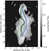 |
Fig. A.1. Stokes I image of 3C 84 showcasing an alternative filamentary morphology identification. The setup is the same as described in Fig. 1. |
Appendix B: Current driven instability
While K-H instabilities have been shown to be able to survive throughout the acceleration and collimation zone and in a highly magnetised regime (see e.g. Nikonov et al. 2023), it is worthwhile to also consider the effect of a CDI (kink instability) on the 3C 84 jet. For such an instability to form, the Kruskal-Shafranov criterion (Bateman 1978) must be satisfied in the ideal magneto-hydrodynamic limit. Specifically, the toroidal component of the magnetic field (Bϕ) must dominate the poloidal (Bp) one, such that:
 (B.1)
(B.1)
where L is the length of the jet. For L ∼ 6 mas in our case and since Bϕ > Bp (Paraschos et al. 2024b), the q < 1 condition is satisfied. Therefore, a CDI could potentially grow in the conditions identified in the 3C 84 jet. At this point it is important to note that, as highlighted in Begelman (1998), current-driven instabilities tend to lead to jet disruption and magnetic reconnection rather than simple wave-like patterns. 3C 84, however, is known for harbouring an ordered magnetic field (Paraschos et al. 2024a) and is also exhibiting such wave-like patterns, as shown in this work.
Overall, there is no simple analytic approach to reliably evaluate the evolution or observational impact of a CDI scenario (Begelman 1998; Bodo et al. 2013). To fully evaluate the growth and potential observational signatures of CDIs, numerical simulations are required – an analysis that lies beyond the scope of this work and will be addressed in a future study.
Alternative identification model predictions
All Tables
All Figures
|
Fig. 1. Stokes I image of 3C 84 showcasing a filamentary morphology. The colour scale is logarithmic and the units are mJy/beam. The dark green ellipse in the lower left corner shows the convolving beam size (0.17 × 0.40) mas. Two threads are superimposed: the green (blue) one traces the filament characterised by higher (lower) flux density. Their widths correspond to the position uncertainty. The computed K-H models are shown with the continuous thin lines, matching the colours of the double helix morphology. The dotted line corresponds to a linear fit of the ridge line with the purpose of determining the position angle (PA = 4.5°) of the jet propagation. The image was turned by −4.5° to align the jet axis with the ordinate. A cutoff at ∼5 mas from the jet apex was implemented, to only include high-S/N areas in our fit. |
| In the text | |
|
Fig. A.1. Stokes I image of 3C 84 showcasing an alternative filamentary morphology identification. The setup is the same as described in Fig. 1. |
| In the text | |
Current usage metrics show cumulative count of Article Views (full-text article views including HTML views, PDF and ePub downloads, according to the available data) and Abstracts Views on Vision4Press platform.
Data correspond to usage on the plateform after 2015. The current usage metrics is available 48-96 hours after online publication and is updated daily on week days.
Initial download of the metrics may take a while.