| Issue |
A&A
Volume 709, May 2026
|
|
|---|---|---|
| Article Number | A9 | |
| Number of page(s) | 10 | |
| Section | Extragalactic astronomy | |
| DOI | https://doi.org/10.1051/0004-6361/202558028 | |
| Published online | 30 April 2026 | |
Gas accretion versus black-hole-merger-driven growth modes of supermassive black holes and implications for the little red dots
1
Istituto Nazionale di Astrofisica (INAF) – Osservatorio Astronomico di Trieste (OATs), Via G.B. Tiepolo 11, I-34143 Trieste, Italy
2
Centro de Ciências Naturais e Humanas – Universidade Federal do ABC, Av. dos Estados 5001 Santo André – SP, 09210-580, Brazil
3
Núcleo de Astrofísica – Universidade Cidade de São Paulo, Rua Galvão Bueno 868 São Paulo – SP, 01506-000, Brazil
4
Instituto de Astronomia, Geofísica e Ciências Atmosféricas – Universidade de São Paulo (IAG-USP), Rua do Matão 1226 São Paulo, 05508-090, Brazil
★ Corresponding author: This email address is being protected from spambots. You need JavaScript enabled to view it.
Received:
7
November
2025
Accepted:
16
February
2026
Abstract
We investigated the growth of central supermassive black holes (SMBHs) in galaxies, with the aim of distinguishing between gas accretion and black-hole (BH) merger-driven growth modes. We performed cosmological hydrodynamical simulations of (50 Mpc)3 comoving volumes, and analyzed how the BH feedback parameters affect the coevolution between SMBHs and their host galaxies. Starting as 105 M⊙ seeds, we find that the BHs initially grow via BH mergers to ∼107 M⊙. Gas accretion onto the BHs is low soon after seeding, and then the accretion rate increases with time and reaches the Eddington rate after 7 − 9 Gyr. The BHs then undergo very fast growth via efficient gas accretion over a time period of 600 − 700 Myr; during this period the BH mass increases 102 − 103 times, causing their predominant growth from 107 M⊙ to (109 − 1010) M⊙. Taking into account the cosmological gas inflows and outflows, SMBHs do not grow to more than 1010 M⊙ by z = 0, which is because of gas depletion from galaxy centers driven by BH feedback. In terms of the coevolution of SMBHs and their host galaxies along the MBH − M★ relation, we find that they initially lie below the relation at earlier epochs and thereby move upward toward the relation. We made some physical implications about the growth of high-z little red dots recently observed by the JWST: the normal-mass SMBHs had predominantly undergone BH-merger-driven evolution, whereas the overmassive BHs underwent periods of Eddington-limited or super-Eddington bursts of gas accretion.
Key words: black hole physics / hydrodynamics / methods: numerical / galaxies: formation / quasars: supermassive black holes
© The Authors 2026
 Open Access article, published by EDP Sciences, under the terms of the Creative Commons Attribution License (https://creativecommons.org/licenses/by/4.0), which permits unrestricted use, distribution, and reproduction in any medium, provided the original work is properly cited.
This article is published in open access under the Subscribe to Open model. This email address is being protected from spambots. You need JavaScript enabled to view it. to support open access publication.
1. Introduction
Supermassive black holes (SMBHs) exist at the centers of active galactic nuclei (AGNs), which liberate enormous amounts of feedback energy powered by the accretion of matter (e.g., Rees 1984; Urry & Padovani 1995). AGNs are widely observed via multi-wavelength observations, starting from the local Universe up to 13.2 Gyr ago (e.g., Fan et al. 2023; Natarajan et al. 2024). SMBHs that had already grown to masses of ≥109 M⊙ were observed in luminous quasars at z ∼ 6, when the Universe was less than 1 Gyr old (e.g., Willott et al. 2003; Yang et al. 2023).
How the SMBHs in AGNs grew to billions of solar masses remains not fully explained, despite progress in our understanding of the SMBH accretion and feedback on the environment (e.g., Alexander et al. 2025). Especially at early epochs, it is difficult to understand how they formed over such short timescales, and there are open issues with various plausible scenarios (e.g., Dijkstra et al. 2008; Inayoshi & Omukai 2012; Matsumoto et al. 2015). Some of the possible mechanisms are: the growth from stellar-mass black holes (BHs) by rapidly enhanced super-Eddington accretion, the formation of direct-collapse massive 105 M⊙ BH seeds soon after the Big Bang (e.g., Volonteri & Rees 2005), or via mergers of intermediate-mass black holes (IMBHs; e.g., Barai & de Gouveia Dal Pino 2019).
Adding to the population of early SMBHs, recent James Webb Space Telescope (JWST) observations revealed 107 − 108 M⊙ BHs at z ∼ 8 − 12 (e.g., Kokorev et al. 2023; Kocevski et al. 2025; Bhatt et al. 2024; Scholtz et al. 2025). Some of these first SMBHs are overmassive in their host galaxy with respect to the z = 0 SMBH-to-stellar mass correlation (e.g., Goulding et al. 2023; Maiolino et al. 2024; Wu et al. 2025). At the same time, a population of normal-mass central SMBHs (with the mean SMBH-to-stellar mass ratio of ∼0.1%, consistent with the local relation) have been detected in z ∼ 3 − 6 AGNs (e.g., Li et al. 2025; Geris et al. 2026) observed by the JWST.
The formation channels of these “normal-mass” and overmassive SMBHs, in terms heavy seeds or super-Eddington accretion onto lighter stellar-mass seeds, have not been identified yet (e.g. Jeon et al. 2025). The very existence of such normal SMBHs together with the overmassive population, imply that there might be diverse pathways for SMBH formation.
Using Sloan Digital Sky Survey and Subaru data, Li et al. (2021) found no significant evolution of the MBH − M★ relation of quasars from z = 0.8 − 0.2, and it remains consistent with the local relation. Graham et al. (2025) argue that the MBH/M★ correlation followed by a population of galaxies (including the JWST-detected high-z little red dots) is dependent on galaxy morphology. Also using JWST observations, Juodžbalis et al. (2026) detected low-luminosity AGNs at z = 1.5 − 9, accreting at likely sub-Eddington ratios, hosted in low-mass (M★ ∼ 108 M⊙) galaxies; where the SMBHs are overmassive relative to the local [MBH − M★] relation, while consistent with the local [MBH − σ★] relation.
Numerical simulations have advanced in parallel to understand these SMBH evolution. Concordance galaxy formation models based on cold dark-matter cosmology widely invoke AGN feedback as a crucial ingredient to self-regulating galaxy and SMBH growth. This has been studied in numerical hydrodynamical simulations (e.g., Di Matteo et al. 2005; Ostriker et al. 2010; Barai et al. 2011; Khandai et al. 2015; Dubois et al. 2016) and semi-analytical models (e.g., Kauffmann & Haehnelt 2000; Somerville et al. 2008; Fontanot et al. 2020).
Related to the goals of our study, Habouzit et al. (2022) showed that the Illustris, TNG100, TNG300, Horizon-AGN, EAGLE, and SIMBA cosmological simulations do not agree on whether BHs at z > 4 are overmassive or undermassive with respect to the MBH − M★ scaling relation at z = 0. Haidar et al. (2022) investigated AGN populations in the Illustris, TNG, Horizon-AGN, EAGLE, and SIMBA simulations compared with current observational constraints in low-mass galaxies, finding that some simulations produce BHs that are too massive. Using (18 Mpc)3 simulations, Kho et al. (2025) found that different BH seeding models lead to different normalizations of the MBH − σ relation. Kho et al. (2025) also found that the BH growth is merger-dominated in low-mass ( ≤ 109 M⊙) galaxies and accretion-dominated in high-mass ( ≥ 109 M⊙) galaxies; this directly influences the MBH − σ evolution.
In our study, we investigated the growth of central SMBHs versus that of their host galaxies by performing (50 Mpc)3 cosmological hydrodynamical simulations, aiming to distinguish between gas accretion versus BH-merger-driven growth modes. We probed the SMBH–galaxy coevolution, in particular that of the BH mass–stellar mass correlation. We also shed light on the growth modes of the overmassive versus normal-mass SMBHs in high-z little red dots recently observed by the JWST.
2. Methodology
We performed (50 Mpc)3 cosmological hydrodynamical simulations using a modified version of the code GADGET-3 (Springel 2005). The code uses the Tree particle-mesh and smoothed particle hydrodynamics methods. The baryonic physical processes occurring in the multiphase interstellar medium, on scales unresolved in cosmological simulations, is modeled using spatially averaged properties describing the medium on scales that are resolved, as described in Sects. 2.1 and 2.2. Our different simulation runs are outlined in Sect. 2.3.
2.1. Cooling, star formation, and SN feedback
We implemented radiative cooling and heating in our work, including metal-line cooling (Wiersma et al. 2009). In this model, net cooling rates are computed via element-by-element by the tracking of 11 atomic species: H, He, C, Ca, O, N, Ne, Mg, S, Si, and Fe. A spatially uniform, time-dependent photoionizing background radiation is considered from the cosmic microwave background and the Haardt & Madau (2001) model for the ultraviolet/X-ray background. The gas is assumed to be dust free, optically thin, and in photoionization equilibrium. Contributions from the 11 elements are interpolated as a function of density, temperature and redshift from tables that were precomputed using the public photoionization code CLOUDY (last described by Ferland et al. 1998).
Star formation (SF) is adopted following the multiphase effective sub-resolution model of Springel & Hernquist (2003). Gas particles with densities above a limiting threshold, ρSF = 0.13 cm−3 (in units of number density of hydrogen atoms), represent cold and hot phase regions of the interstellar medium. Stellar evolution and chemical enrichment are computed for the 11 elements (Tornatore et al. 2007). Each star particle is treated as a simple stellar population. Given a stellar initial mass function, the mass of the simple stellar population is varied in time following the death of stars, and accounting for stellar mass losses. A fixed stellar initial mass function (Chabrier 2003) is included, in the mass range (0.1 − 100) M⊙. Stars within a mass interval of [8 − 40] M⊙ first become supernovae (SNe) before turning into stellar-mass BHs at the end of their lives, while stars of mass > 40 M⊙ are allowed to directly end in BHs without contributing to gas enrichment.
Feedback from SNe is incorporated in the kinetic form, assuming a mass ejection rate, ṀSN, proportional to the star formation rate (SFR, or Ṁ★):
 (1)
(1)
The mass-loading factor of SN wind is taken as η = 2 (e.g., Tornatore et al. 2007; Barai et al. 2013; Melioli et al. 2013), following observations revealing that SN-driven outflow rates are comparable to or higher than the SFRs of galaxies (e.g., Martin 1999; Bouché et al. 2012). The SN wind’s kinetic power is a fixed fraction, χ, of the SN internal energy rate:
 (2)
(2)
Here, vSN is the SN wind velocity, and ϵSN is the average energy released by SNe for each M⊙ star formed under the instantaneous recycling approximation. For our adopted Chabrier (2003) power-law initial mass function, ϵSN = 1.1 × 1049 erg  . Combining the above expressions, vSN can be rewritten as vSN = (2χϵSN/η)1/2. Following a series of studies (e.g., Tornatore et al. 2007; Tescari et al. 2011; Barai et al. 2013), and unlike Springel & Hernquist (2003), we chose vSN as a free parameter. We adopted a constant-velocity outflow with an SN wind velocity of vSN = 350 km/s (as was done in, e.g., Tornatore et al. 2007; Barai et al. 2015, and Biffi et al. 2016).
2.2. BH accretion and feedback
We identified galaxies in our simulations by executing a friends-of-friends (FOF) group finder at time intervals of a multiplicative factor 1.4 of the cosmological scale factor a, or anext/aprev = 1.4. Massive galaxies (i) with a total halo mass higher than 1010 M⊙, (ii) with a stellar mass higher than 5 × 10⁷ M⊙, (iii) with gas mass equal or larger than 10% of stellar mass, and (iv) not containing a BH yet, were selected. A BH of initial mass MBH = 105 M⊙ was seeded at the center of each such massive galaxy.
Gas was considered to accrete onto a BH according to the Bondi–Hoyle–Lyttleton accretion rate (ṀBondi: Hoyle & Lyttleton 1939; Bondi 1952):
 (3)
(3)
where G is the gravitational constant, cs is the sound speed, ρ is the gas density, and v is the velocity of the BH relative to the gas. The Bondi accretion numerical boost factor (e.g., Springel et al. 2005; Johansson et al. 2008; Dubois et al. 2013) was set as αB = 1. Furthermore, accretion was limited to the Eddington mass-accretion rate (ṀEdd): ṀBH = min (ṀBondi, ṀEdd). The Eddington mass-accretion rate can be obtained from the Eddington luminosity via the usual expression,
 (4)
(4)
where mp is the mass of a proton, c is the speed of light, and σT is the Thomson scattering cross-section for an electron.
Feedback energy was distributed in the surrounding gas according to
 (5)
(5)
Here, ϵr is the radiative efficiency and ϵf is the feedback efficiency. We adopted ϵr = 0.1, which assumes radiatively efficient accretion onto a Schwarzschild BH (Shakura & Sunyaev 1973).
Kinetic BH feedback was included (Barai et al. 2014, 2016), whereby the neighboring gas is pushed outward with a velocity of vw and mass-outflow rate of Ṁw. Using the conservation of energy,  , and Eq. (5), the BH kinetic feedback mass-outflow rate can be written as
 (6)
(6)
We used the values ϵf = 0.05 and vw = 5000 km/s.
The BH kinetic-feedback energy was distributed to the gas within a distance of hBH from the BH. A bicone volume was defined around the BH with a slant height of hBH and half-opening angle of 45°. The bicone-axis direction was randomly assigned during BH seeding and remained fixed thereafter for each BH. The total gas mass within the bicone  was computed. A probability was calculated for the i-th gas particle inside the bicone, in a time step of Δt:
 (7)
(7)
where Ṁw is the mass-outflow rate obtained from Eq. (6). A random number, xi, uniformly distributed in the interval [0, 1], was drawn. If xi < pi, the gas particle was imparted a velocity boost via AGN wind, such that
 (8)
(8)
Here, vold and vnew are the old and new velocities of the gas particle. The AGN wind direction,  was considered radially outward from the BH.
We did not incorporate any scheme for BH repositioning or pinning. Thus contrary to Barai et al. (2018), each BH was not repositioned at each time step to the location of the minimum gravitational potential of its host galaxy.
When galaxies merge during hierarchical structure assembly, their hosted central BHs merge as well. In the numerical algorithm, two BH particles were allowed to merge to form a single BH when the distance between them was smaller than the smoothing length of either one and their relative velocity was below the local sound speed (e.g., Sijacki et al. 2007; Di Matteo et al. 2012). The final merged BH was considered to have a mass equal to the sum of the BH masses and a velocity along the center of mass of the initial two merging BHs. To impart kinetic-feedback energy, the merged BH retained the bicone axis direction of the more massive initial BH.
2.3. Simulations
We performed cosmological hydrodynamical simulations of (50 Mpc)3 comoving volumes. Our standard resolution is eight simulations using 2563 dark matter and 2563 gas particles in the initial condition. The dark-matter particle mass is mDM = 2.47 × 10⁸ M⊙, and the gas particle mass is mgas = 4.61 × 10⁷ M⊙. The gravitational softening length was set as Lsoft = 3.3 kpc comoving. The MUSIC1 software (Hahn & Abel 2011) was used to generate the initial condition at z = 100. The concordance flat Λ cold dark matter cosmological model was used, with the density parameters: ΩM, 0 = 0.3089, ΩΛ, 0 = 0.6911, ΩB, 0 = 0.0486, H0 = 67.74 km s−1 Mpc−1 (Ade et al. 2016, results XIII). Starting from z = 100, the boxes were subsequently evolved up to z = 0, with periodic boundary conditions.
We executed a series of simulations, with characteristics listed in Table 1. All the runs incorporated metal cooling, chemical enrichment, and SF. The first run, SFonly, had no SN feedback nor BHs. SN feedback was additionally included in the second and subsequent runs, while the remaining runs also included BHs. The runs are listed below.
-
SN: No BH present. This is a control simulation in which only cooling, SF, chemical evolution and SNe feedback were implemented.
-
BHsXeYvZ: With BH accretion and feedback. The symbols X, Y, and Z indicate the parameters being varied between the simulations in the following way: MBHseed = 10X M⊙; BH feedback efficiency, ϵf = Y; and BH kinetic-feedback kick velocity, vw = Z × 1000 km/s.
Simulation runs and parameter values changed in each case.
Halos were identified by executing a FOF group finder on the fly within our simulations. Galaxies were tracked using the subhalo finder SubFind, which associates substructures with FOF halos. The location of the gravitational potential minimum of the dark-matter subhalo was considered as the center of each galaxy. The halo mass (Mhalo) of a galaxy and its virial radius in comoving coordinates (R200) are related such that R200 encloses a density 200 times the mean comoving matter density of the Universe:
 (9)
(9)
where ρcrit = 3H02/(8πG) is the present critical density. The galaxy stellar mass was considered as the mass of all star particles inside the subhalos obtained by the subhalo finder SubFind.
3. Results and discussion
3.1. MBH versus M★ relation buildup with cosmic time
The cosmic buildup of the BH mass, MBH, versus stellar mass, M★, of our simulated galaxies is shown in Fig. 1. Six epochs of our standard run, BHs5e0.1v5, are plotted (which gives the best fit to the observational Marconi & Hunt (2003)z = 0 correlation), one each at z = 5, 3, 2, 1, 0.5, 0. Observational data are overplotted as the black lines, indicating the BH mass versus stellar bulge mass relationships at different epochs. Local galaxies (z = 0) are represented by the solid line, MBH/M★ = 0.002 (Marconi & Hunt 2003), as well as from Reines & Volonteri (2015) as the dotted line and from McConnell & Ma (2013) as the dashed line. The ratio is observed to be steeper at high-z. Bright z ∼ 6 quasars, observed in the far-IR and CO, lie along the dash-dotted line: median MBH/M★ = 0.022 (Wang et al. 2010).
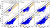 |
Fig. 1. Cosmic buildup of BH mass versus stellar mass of our simulated galaxies, denoted by the blue circles, in run BHs5e0.1v5, each panel indicating one redshift: z = 5, 3, 2, 1, 0.5, 0. The black lines mark the observed BH mass versus galaxy stellar mass relation for local galaxies, showing correlation with the bulge mass as solid (Marconi & Hunt 2003), dashed (McConnell & Ma 2013), and dotted (Reines & Volonteri 2015) lines. The relation for quasars at z ∼ 6 (Wang et al. 2010) is shown as the dash-dotted line. |
We find that the slope of the [MBH − M★] correlation remains almost constant in our simulations, and there is an intercept evolution with cosmic time. Noting that the observational relation by Reines & Volonteri (2015) lies somewhat lower than that by Marconi & Hunt (2003) and McConnell & Ma (2013), our simulated galaxies are found to follow these different relations at distinct redshifts. At earlier epochs z = 5 − 3, the BHs more closely follow the Reines & Volonteri (2015) correlation; at z = 2 − 1, the BHs are in between the two relations; while at current epochs z = 0 they lie more on the Marconi & Hunt (2003) and McConnell & Ma (2013) correlations.
3.2. Mass growth of the SMBHs: Merger-driven versus accretion-driven regimes
In our simulations, the first BHs were seeded at z ∼ 9. Generally, in such cosmological simulations, the redshift of the seeding of BHs is a quantity dependent on the box size and numerical resolution. For our standard resolution runs, z = 8.5 − 9 is the first cosmic epoch during which a massive halo reaches Mhalo = 1010 M⊙; and a BH of 105 M⊙ was seeded at its center. More BHs were seeded at later epochs following the prescription described in Sect. 2.2.
We find that none of the first seeds (BHs that are seeded at z ∼ 9) grow to become one of the most massive BHs at z = 0. The BHs that become the most massive are actually seeded at later epochs: z ∼ 2 − 5. This is because of the different BH growth modes, as described next.
The growth with redshift of some of the massive BHs in our BHs5e0.1v5 run are plotted in Fig. 2. Each BH started from an initial seed of MBH = 105 M⊙. The subsequent mass growth is due to a merger with other BHs (revealed as vertical rises in MBH) and gas accretion (visualized as the positive-sloped regions of the MBH versus z curve).
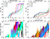 |
Fig. 2. Growth with redshift of BH mass (top row) and Eddington accretion ratio = ṀBH/ṀEdd (bottom row) of some of the massive BHs in our standard simulation BHs5e0.1v5. Left column: six most massive SMBHs with the final mass MBH(z = 0) > 109 M⊙. Right column: six IMBHs of MBH(z = 0) = (107 − 108) M⊙. |
We quantified the driving mechanism of the mass growth of the BHs using a limiting Eddington accretion ratio of 0.1. If ṀBH/ṀEdd ≥ 0.1, it was considered an accretion-driven mass-growth regime; while ṀBH/ṀEdd < 0.1 was considered part of a merger-driven growth regime. The results of these two growth regimes are plotted in Fig. 3.
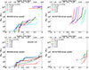 |
Fig. 3. Growth of BH mass due to mergers or accretion of the same BHs as plotted in Fig. 2: the six most massive BHs (top row) and six IMBHs (bottom row) from our standard simulation BHs5e0.1v5. Left column: merger-driven mass-growth regime. Right column: accretion-driven mass-growth regime; the two regimes are distinguished with a limiting Eddington accretion ratio = 0.1, as described in Sect. 3.2. |
We find that the initial growth from 105 M⊙ seeds to ∼107 M⊙ occurs predominantly via BH mergers (left two panels of Fig. 3). Our result is consistent with other cosmological simulations (Bhowmick et al. 2024, 2025), which found that the growth of BHs of mass (105 − 107) M⊙ at z ≥ 4 is merger driven, with a relatively small contribution from gas accretion.
We find that for the BHs that become supermassive with mass ≥109 M⊙, their final growth occurs over a period of 600 − 700 Myr dominated by efficient gas accretion (top-right panel of Fig. 3). This period corresponds to an Eddington-limited accretion, where the Eddington ratio = 1 (bottom-left panel of Fig. 2). The BH mass increases by a factor 102 − 103, which increases their masses from 107 M⊙ to (109 − 1010) M⊙ in this short time period of 600 − 700 Myr. The trend we obtained that gas accretion becomes the dominant growth mode for more massive BHs is consistent with other cosmological simulations (Bhowmick et al. 2024; Kho et al. 2025), where the relative contribution from gas accretion increases for more massive BHs and at lower redshifts.
In our simulations, after the Eddington-limited accretion period, the SMBHs have a flat mass evolution with redshift (top-left panel of Fig. 3); i.e., they stop growing up to z = 0. We speculate that such a final growth halt happens because of gas depletion from galaxy centers.
The cosmic epoch of the rapid efficient gas accretion is seen to vary depending on the SMBH, as can be seen in the top-right panel of Fig. 3. The red curve grows from MBH = 7 × 10⁶ M⊙ at z = 0.4 to MBH = 6 × 10⁹ M⊙ at z ∼ 0.3 and has a passive evolution thereafter. The cyan curve grows from MBH = 4 × 10⁶ M⊙ at z = 0.1 to MBH = 5 × 10⁹ M⊙ at z = 0.05. The consistent feature among all the BHs is that the final growth inevitably happens within a time period of 600 − 700 Myr (as described in the previous paragraph). We argue the physical reason behind such BH growth behavior is the influence of gas supply to the host galaxy center and subsequent efficient gas accretion onto the BH, leading to gas depletion within 700 Myr.
The right column of Fig. 2 and the bottom row of Fig. 3 present six IMBHs, those that reached MBH(z = 0) = (107 − 108) M⊙ at the present epoch. We find that their growth happened primarily via BH mergers (indicated by vertical rises of MBH). Their accretion ratio remains sub-Eddington. At z < 0.05, some of them (blue, green, red, and orange curves) reach an Eddington ratio = 1 for 100 − 200 Myr, but this soon becomes sub-Eddington because of gas depletion.
3.2.1. Implications for the little red dots
We can apply our numerical simulation results of SMBH growth to the z > 4 little red dots recently observed by the JWST (e.g., Labbé et al. 2023; Killi et al. 2024; Matthee et al. 2024). Little red dots are sources with a compact morphology and red optical color; they present a V-shaped spectral energy distribution and spectroscopic broad Balmer emission lines. The observed emission of the little red dots likely consists of an AGN component (e.g., Greene et al. 2024; Xiao et al. 2025) with BH mass in the range of MBH = 106 − 108 M⊙ and/or a compact starburst (e.g., Pérez-González et al. 2024; Williams et al. 2024).
With the AGN source interpretation, the little red dots represent low-luminosity AGNs (e.g., Ma et al. 2025), which are often obscured by dust (e.g., Fujimoto et al. 2022; Akins et al. 2023) in the early Universe. These high-z faint AGNs represent a surprisingly abundant population at z > 5, with a volume number density ∼100 times the extrapolated quasar UV luminosity function (e.g., Matthee et al. 2024; Lin et al. 2024). As a fraction of the galaxy population, Harikane et al. (2023) found that ∼5% of galaxies at z = 4 − 7 are type-1 AGNs with broad lines, which is thus a higher fraction than z ∼ 0 galaxies with similar luminosities.
The host-galaxy stellar masses of the little red dots can be inferred from observations. Considering the [MBH − M★] correlation, the high-z BHs, those hosted by the little red dots, lie above the local correlation. This implies a quickened and efficient BH growth at early epochs in sources being observed as little red dots (Harikane et al. 2023). Interpreting with our numerical simulation results on the growth modes of the BHs presented Sect. 3.2: the high-z BH growth observed in studies such as Harikane et al. (2023) must have been dominated by efficient gas accretion close to the Eddington limit.
Our implication of the little red dots assumes the AGN source interpretation. These JWST-detected early SMBHs at z ∼ 4 − 12 comprise some BHs that are overmassive (e.g., Goulding et al. 2023; Wu et al. 2025) in their host galaxy, as well as some normal-mass SMBHs (e.g., Li et al. 2025; Geris et al. 2026) with respect to the local [MBH − M★] correlation. Applying our results to these high-z AGNs in little red dots, we assert that the normal-mass SMBHs had predominantly undergone BH-merger-driven evolution, whereas the overmassive BHs underwent periods of Eddington-limited or super-Eddington bursts of efficient gas accretion. The high nuclear gas density in the galaxies forming in the early Universe lead to vigorous gas accretion onto BHs turning them overmassive. These trends also imply that the [MBH − M★] relation becomes more defined (i.e., with a smaller scatter) at lower redshifts.
3.3. Cosmic evolution along the [MBH − M★] diagram
The right panels of Fig. 4 show the evolution track with cosmic time of the BH mass versus host galaxy stellar mass of the six most massive BHs (top row) and six IMBHs (bottom row); these are same BHs that are plotted in Fig. 2. The corresponding redshift evolution of the host galaxy’s stellar mass of each BH is shown in the left panels of Fig. 4. We can visualize (top-left panel) that each SMBH mostly stays in the same host galaxy, whose stellar mass, MStellar, builds up with time steadily. At a few epochs the host galaxy undergoes merger(s) to form a larger galaxy, when the MStellar increases sharply. There can be occasions when the BH migrates to a less massive host galaxy for a short period of time, which happens with bh6 (the cyan curve) at z ∼ 1.8.
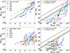 |
Fig. 4. Left column: Buildup with redshift of the stellar mass of the host galaxy of the six most massive BHs (top row) and six IMBHs (bottom row); the same BHs that were plotted in Fig. 2, distinguished by the plotting colors. Right column: Redshift track or the evolution with cosmic time of the BH mass versus host galaxy stellar mass of the BHs. The observed BH mass versus galaxy stellar mass relation of local galaxies (Marconi & Hunt 2003) is shown as the dashed black line and z = 6 quasars (Wang et al. 2010) are shown as the solid black line. |
The temporary migration of a BH from a more massive host galaxy to a less massive galaxy happens much more frequently with the IMBHs (bottom-left panel); bh8, bh9, bh10, and bh12 demonstrate such migration signatures when the stellar mass decreases abruptly for some time. Such host migration happens more frequently for the IMBHs as compared to the SMBHs because of a greater influence of dynamical forces in the lower-mass IMBHs.
In the right panels of Fig. 4, each track starts at a point in the bottom left that corresponds to an epoch when the BH was seeded, at z ∼ 3 − 5; and it evolves up to the top right point, which corresponds to z = 0. At the time of their seeding the BHs start below the observed [MBH − M★] correlation, and they slowly evolve to the z = 0 correlation first, and some BHs overshoot it eventually continuing toward the z = 6 correlation. The SMBHs displayed in the top-right panel of Fig. 4 have reached, or overshooted, the observed correlation at z = 0. While the IMBHs (bottom-right panel) still lies below the observed correlation.
3.4. Environment of the SMBHs
The evolution of the gas environment around an assembling massive BH is plotted in Fig. 5. It displays gas overdensity (i.e., the ratio between the gas density and the cosmological mean baryon density of the Universe) in our simulation BHs5e0.1v5 at six epochs: z = 3, 2, 1, 0.5, 0.2, and 0. The BH that would become most massive in this run at z = 0 is backtracked, and each panel shows a projected (2000 h−1 kpc)3 comoving volume around the location of this BH. The black circle is the virial radius R200 (defined in Eq. (9)) of the host galaxy of the back-tracked BH, the red circles depict the R200 of the galaxies with the mass range Mhalo > 1012 M⊙, and the blue circles show the R200 of (1011 < Mhalo < 1012) M⊙ galaxies. The spatial locations of all the BHs inside the plotted region can be visualized with the red cross symbols, with the symbol size proportional to BH mass.
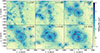 |
Fig. 5. Gas overdensity in our standard simulation BHs5e0.1v5 at six cosmic epochs z = 3, 2, 1, 0.5, 0.2, 0. The BH that would become most massive at z = 0 is backtracked, and each panel shows a projected (2000 h−1 kpc)3 comoving volume around the location of this BH. The red cross symbols indicate the positions of all the BHs inside the plotted region, where the symbol size is proportional to BH mass. The black circle is the virial radius, R200, of the host galaxy of the backtracked BH, the red circles depict the R200 of galaxies with the mass range Mhalo > 1012 M⊙, and the blue circles show the R200 of (1011 < Mhalo < 1012) M⊙ galaxies. |
In the top panels of Fig. 5, we can see the cosmological large-scale-structure megaparsec-scale filaments, consisting of dense (blue and dark-blue regions) gas. The galaxies (blue and red circles) lie along the filaments, or at the high-density intersections of the filaments, and finally in the galaxy cluster region which formed at z = 0. The clustering of halos is visible in all the panels; at z = 3, 2, 1 the halos are in the process of formation along cosmological large-scale-structure filaments, while at z = 0.5, 0.2 the halos formed an overdense protocluster region at the center of the plotted volume, which evolved to a dense galaxy cluster region at z = 0. Thus in this simulation, the most-massive BH of MBH(z = 0) = 2 × 10¹⁰ M⊙ lies at the center of a galaxy cluster.
3.5. Influence of AGN feedback model parameters
The BH mass versus galaxy stellar mass correlation obtained in seven of our simulations at the current epoch z = 0 is presented in Fig. 6. We find a relatively large scatter in the [MBH − M★] correlation of our simulated galaxies, which is comparable to the scatter found in observations (e.g., Reines & Volonteri 2015). Our standard simulation BHs5e0.1v5 with MBHseed = 105 M⊙, ϵf = 0.1, and vw = 5000 km/s is able to reproduce the observational (Marconi & Hunt 2003) z = 0 correlation well.
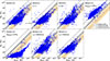 |
Fig. 6. BH mass versus stellar mass of the galaxies obtained in our simulations, at the current epoch z = 0, each panel displaying one distinct run. We indicate the observed BH mass versus galaxy stellar mass relation for local galaxies showing the correlation with the bulge mass as the solid (Marconi & Hunt 2003), dashed (McConnell & Ma 2013), and dotted (Reines & Volonteri 2015) black lines; we show z ∼ 6 quasars (Wang et al. 2010) as the dash-dotted black line. |
Among the relevant BH sub-grid model parameter variations, the largest impact is seen with the BH seed mass. With a higher MBHseed = 106 M⊙ (run BHs6e0.1v5), the resulting BHs are too massive and overshoot the local relation. On seeding with a lower seed mass of MBHseed = 104 M⊙ (run BHs4e0.1v5), the resulting BHs do not grow enough and remain below the local one. There is a relatively lower impact of the BH feedback efficiency and feedback kick velocity. With ϵf = 1 (run BHs5e1v5) and with vw = 1000 km/s (run BHs5e0.1v1), the BHs lie slightly below the local [MBH − M★] correlation. With ϵf = 0 (run BHs5e0v5) and with vw = 10 000 km/s (run BHs5e0.1v10), the BHs lie slightly above the z = 0 local relation.
It is worthwhile to note that the simulation with ϵf = 0 (run BHs5e0v5) is one with no BH feedback because the efficiency (viz. Eq. (5)) was set to zero, as a test case. From the top row in the third panel of Fig. 6, we thus see that even with no BH feedback some kind of [MBH − M★] correlation is generated in the simulation.
3.6. Star formation rate
We computed the star formation rate density (SFRD; in M⊙ yr−1 Mpc−3) by summing over all the SF occurring in each simulation box at a time and dividing it by the time-step interval and the box volume. The global SFRD as a function of redshift is presented in Fig. 7 for eight of our simulations. Observational data limits are shown for comparison; they were taken from Cucciati et al. (2012), and the compilations therein originally from Pérez-González et al. (2005), Schiminovich et al. (2005), Bouwens et al. (2009), Reddy & Steidel (2009), Rodighiero et al. (2010), van der Burg et al. (2010), and Bouwens et al. (2012). The SFRD from these observations continues to grow from early cosmic epochs at z < 10 and has a peak around z ∼ 2 − 3.
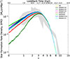 |
Fig. 7. SFRD integrated over the whole simulation volume as a function of redshift, with the different simulation runs labeled by the colors and line styles. The gray shaded region denotes a combination of observational SFRD data range from Cucciati et al. (2012), and the compilations therein originally from Pérez-González et al. (2005), Schiminovich et al. (2005), Bouwens et al. (2009), Reddy & Steidel (2009), Rodighiero et al. (2010), van der Burg et al. (2010), and Bouwens et al. (2012). |
In our simulations, we find that the SFRD rises with time from early epochs z ∼ 10 and reaches a maximum SFRD in the form of a wide peak at z ∼ 2 − 3, and the SFRD decreases at z < 3; this overall trend is consistent with the observations. Star formation occurs inside galaxies, where cosmic large-scale-structure gas inflows and cools. The presence of a central SMBH helps to quench SF, because a fraction of gas is ejected out and/or heated by BH feedback, and a small fraction might be accreted onto the BH.
We considered the SN run (yellow curve) without BHs as the baseline, and we compared other simulations with it to estimate the impact of BH feedback. Note that in the BHs5e0v5 run (light green curve), no BH feedback was implemented, or ϵf = 0; here, the SF remains the same as in the SN run. However, the growth of BHs by gas accretion and mergers is present in the simulation BHs5e0v5. As the SFRD in runs SN and BHs5e0v5 remains the same, we conclude that gas removal by accretion onto BHs plays only a very minor role in suppressing SF, and the major role is played by BH-feedback-induced removal and heating of gas.
We find that the physical processes of BH accretion and feedback cause a quenching of the SFRD compared to the SN case (yellow curve in Fig. 7) at cosmic epochs of z ≤ 4. The reduction of SFRD factors at z = 0 for the different simulations range from 1.3 to 15 times.
To explore the galaxy main sequence, we plot the SFR (in M⊙/yr) versus stellar mass (M★) of all the galaxies within six of our simulations in Fig. 8, at the epochs z ∼ 5 and z ∼ 2. We also show observational data from Salmon et al. (2015) of star-forming galaxies at z = 4, 5, and 6: the best-fit relation of SFR versus M★, as written in their Eq. (6), with parameters given in their Table 4; and observations from Santini et al. (2017) in different redshift bins within z = 1.3 − 6: the data points are taken from their Table 1.
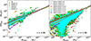 |
Fig. 8. SFR versus stellar mass of the galaxies in our simulations at the epoch z ∼ 5 (left) and z ∼ 2 (right). The filled circles are our simulation results and the plotting colors distinguish results from different runs. The observational results of SFR versus stellar mass relation are indicated for star-forming galaxies at z = 4, 5, 6 (Salmon et al. 2015) as solid lines and galaxies in different redshift bins within z = 1.3 − 6 (Santini et al. 2017) as dashed lines with square plotting symbols. |
We find that our simulated galaxies are consistent with the [SFR–M★] relations showing the observational main sequence of star-forming galaxies. There is, however, a large scatter in our SFR versus M★ correlation.
4. Conclusions and summary
How the central SMBHs grew to billions of solar masses and produced the varied populations of AGNs that we observe is not fully known. Especially at early epochs, luminous z ∼ 6 quasars are observed to host 109 M⊙ SMBHs when the Universe was < 1 Gyr old. It is challenging to understand how they formed over such short timescales, with various possible theories: growth from stellar mass seed BHs by rapidly enhanced super-Eddington accretion, formation of direct-collapse heavy 105 M⊙ BH seeds soon after the Big Bang, or via mergers of IMBHs.
Adding to the population of early SMBHs, recent JWST observations detected many SMBHs at z ∼ 4 − 12 that are overmassive in their host galaxy, as well as some SMBHs that are normal-mass with respect to the local MBH − M★ correlation. The exact formation channels of these diverse populations of normal-mass and overmassive SMBHs are unknown.
We investigated the growth of SMBHs versus host galaxies, as well as their feedback, by performing cosmological hydrodynamical simulations. Using a modified version of the smoothed particle hydrodynamics code GADGET-3, we simulated (50 Mpc)3 comoving volumes, with a mass resolution of 4.61 × 10⁷ M⊙ for gas particles, from z = 100 up to z = 0. The simulations include the sub-resolution physics of radiative cooling, SF, stellar evolution, chemical enrichment, SNe feedback, AGN accretion, and feedback. We probed the BH-galaxy co-evolution in terms of the BH mass–stellar mass correlation.
We executed a series of simulations: two of them are control cases; one with SF-only and one also including SNe feedback; the other runs included BHs as well. We explored different parameter variations of the BH sub-resolution models: MBHseed = (104, 105, 106) M⊙, ϵf = 0, 0.1, 1, the outflow velocity for BH kinetic feedback: vw = 1000, 5000, 10 000 km/s.
Based on our simulations, in our study we find the following:
-
The initial growth from 105 M⊙ seeds to ∼107 M⊙ BHs occurs predominantly via BH mergers.
-
Gas accretion onto the BHs is initially low, with highly sub-Eddington accretion rates (ṀBH/ṀEdd <; 0.001). ṀBH increases with time and reaches the Eddington rate after 7 − 9 Gyr. The BHs then undergo very fast growth via Eddington-limited (or Eddington ratio = 1) gas accretion. Within a period of 600 − 700 Myr, the BHs grow from 107 M⊙ to (109 − 1010) M⊙.
-
SMBHs (those reaching 109 − 1010 M⊙ at z = 0) have had their predominant growth over a period of 600 − 700 Myr via strong gas accretion. During this period, the BH mass increases by a factor 102 − 103. We argue that such BH growth behavior results from the influence of gas supply to the host galaxy center, and subsequent efficient gas accretion onto the BH; which leads to central gas depletion within 700 Myr.
-
After the Eddington-limited gas accretion growth to ∼109 − 1010 M⊙, the SMBHs stop growing and maintain the same mass up to z = 0. This final growth halt happens because of gas depletion from galaxy centers.
-
The most-massive population of BHs have grown to MBH ∼ 1010 M⊙ at z = 0. BHs do not grow to more than 1010 M⊙, because of gas removal by AGN-feedback-driven self-regulation. Some BHs may have reached this maximum mass 2 or 3 Gyr ago.
-
Applying our results to the JWST-detected high-z little red dots, we argue that the normal-mass SMBHs had predominantly undergone BH-merger-driven evolution, whereas the overmassive BHs underwent periods of Eddington-limited or super-Eddington bursts of gas accretion.
-
Our simulations probe galaxies with a stellar mass of M★ = (108 − 1012) M⊙. The SFRD (M⊙ yr−1 Mpc−3) versus redshift evolution, as well as the main sequence of the SFR–stellar mass relation of these galaxies, are consistent with observations. Star formation is quenched at z = 3 − 0, and the SFRD is reduced by factors 1.3 − 15.
-
Gas removal by accretion onto BHs plays only a very minor role in suppressing SF, and the major role is played by BH-feedback-induced removal and/or heating of gas.
We deduce that supermassive 109 − 1010 M⊙ BHs have had their predominant growth over a period of 600 − 700 Myr via efficient gas accretion, from the gas supply to the host galaxy center, when the BH mass increases 102 − 103 times. BH mergers play a minor role compared to gas accretion for SMBH growth. SMBHs do not grow to more than 1010 M⊙, because of gas depletion from galaxy centers driven by AGN feedback.
Acknowledgments
P.B. is most grateful to Volker Springel and Klaus Dolag for allowing to use the GADGET-3 code. The simulations were performed at the supercomputing cluster GAPAE of IAG-USP. P.B. acknowledges useful discussions with Giuseppe Murante, Matteo Viel, Luca Tornatore, Stefano Borgani, Gian Luigi Granato, Pierluigi Monaco, Simona Gallerani, and Andrea Ferrara. The work has been supported by the Brazilian funding Agency FAPESP (grants 2016/01355-5 and 2016/22183-8); and the Italian Ministry of University and Research (MUR) Missione 4 “Istruzione e Ricerca” – Componente C2, Investimento 1.1 Fondo per il Programma Nazionale di Ricerca e Progetti di Rilevante Interesse Nazionale (PRIN), the PRIN 2022 PNRR grant under the National Recovery and Resilience Plan (PNRR): project P2022ZLW4T “Next-generation computing and data technologies to probe the cosmic metal content” (ref. P. Barai).
References
- Ade, P. A., Aghanim, N., Arnaud, M., et al. 2016, A&A, 594, A13 [NASA ADS] [CrossRef] [EDP Sciences] [Google Scholar]
- Akins, H. B., Casey, C. M., Allen, N., et al. 2023, ApJ, 956, 61 [NASA ADS] [CrossRef] [Google Scholar]
- Alexander, D. M., Hickox, R. C., Aird, J., et al. 2025, New Astron. Rev., 101, 101733 [Google Scholar]
- Barai, P., & de Gouveia Dal Pino, E. M. 2019, MNRAS, 487, 5549 [NASA ADS] [CrossRef] [Google Scholar]
- Barai, P., Martel, H., & Germain, J. 2011, ApJ, 727, 54 [Google Scholar]
- Barai, P., Viel, M., Borgani, S., et al. 2013, MNRAS, 430, 3213 [Google Scholar]
- Barai, P., Viel, M., Murante, G., et al. 2014, MNRAS, 437, 1456 [NASA ADS] [CrossRef] [Google Scholar]
- Barai, P., Monaco, P., Murante, G., et al. 2015, MNRAS, 447, 266 [Google Scholar]
- Barai, P., Murante, G., Borgani, S., et al. 2016, MNRAS, 461, 1548 [NASA ADS] [CrossRef] [Google Scholar]
- Barai, P., Gallerani, S., Pallottini, A., et al. 2018, MNRAS, 473, 4003 [NASA ADS] [CrossRef] [Google Scholar]
- Bhatt, M., Gallerani, S., Ferrara, A., et al. 2024, A&A, 686, A141 [NASA ADS] [CrossRef] [EDP Sciences] [Google Scholar]
- Bhowmick, A. K., Blecha, L., Torrey, P., et al. 2024, MNRAS, 533, 1907 [Google Scholar]
- Bhowmick, A. K., Blecha, L., Kelley, L. Z., et al. 2025, ApJ, 991, 81 [Google Scholar]
- Biffi, V., Borgani, S., Murante, G., et al. 2016, ApJ, 827, 112 [NASA ADS] [CrossRef] [Google Scholar]
- Bondi, H. 1952, MNRAS, 112, 195 [Google Scholar]
- Bouché, N., Hohensee, W., Vargas, R., et al. 2012, MNRAS, 426, 801 [CrossRef] [Google Scholar]
- Bouwens, R., Illingworth, G., Franx, M., et al. 2009, ApJ, 705, 936 [Google Scholar]
- Bouwens, R. J., Illingworth, G., Oesch, P., et al. 2012, ApJ, 754, 83 [Google Scholar]
- Chabrier, G. 2003, PASP, 115, 763 [Google Scholar]
- Cucciati, O., Tresse, L., Ilbert, O., et al. 2012, A&A, 539, A31 [NASA ADS] [CrossRef] [EDP Sciences] [Google Scholar]
- Di Matteo, T., Springel, V., & Hernquist, L. 2005, Nature, 433, 604 [NASA ADS] [CrossRef] [Google Scholar]
- Di Matteo, T., Khandai, N., DeGraf, C., et al. 2012, ApJ, 745, L29 [NASA ADS] [CrossRef] [Google Scholar]
- Dijkstra, M., Haiman, Z., Mesinger, A., et al. 2008, MNRAS, 391, 1961 [NASA ADS] [CrossRef] [Google Scholar]
- Dubois, Y., Pichon, C., Devriendt, J., et al. 2013, MNRAS, 428, 2885 [NASA ADS] [CrossRef] [Google Scholar]
- Dubois, Y., Peirani, S., Pichon, C., et al. 2016, MNRAS, 463, 3948 [Google Scholar]
- Fan, X., Bañados, E., & Simcoe, R. A. 2023, ARA&A, 61, 373 [NASA ADS] [CrossRef] [Google Scholar]
- Ferland, G., Korista, K., Verner, D., et al. 1998, PASP, 110, 761 [NASA ADS] [CrossRef] [Google Scholar]
- Fontanot, F., De Lucia, G., Hirschmann, M., et al. 2020, MNRAS, 496, 3943 [CrossRef] [Google Scholar]
- Fujimoto, S., Brammer, G. B., Watson, D., et al. 2022, Nature, 604, 261 [NASA ADS] [CrossRef] [Google Scholar]
- Geris, S., Maiolino, R., Isobe, Y., et al. 2026, MNRAS, 545, staf1979 [Google Scholar]
- Goulding, A. D., Greene, J. E., Setton, D. J., et al. 2023, ApJ, 955, L24 [NASA ADS] [CrossRef] [Google Scholar]
- Graham, A. W., Chilingarian, I., Nguyen, D. D., et al. 2025, PASA, 42 [Google Scholar]
- Greene, J. E., Labbe, I., Goulding, A. D., et al. 2024, ApJ, 964, 39 [CrossRef] [Google Scholar]
- Haardt, F., & Madau, P. 2001, in Clusters of Galaxies and the High Redshift Universe Observed in X-rays, eds. D. M. Neumann, & J. T. V. Tran, 64 [Google Scholar]
- Habouzit, M., Onoue, M., Bañados, E., et al. 2022, MNRAS, 511, 3751 [NASA ADS] [CrossRef] [Google Scholar]
- Hahn, O., & Abel, T. 2011, MNRAS, 415, 2101 [Google Scholar]
- Haidar, H., Habouzit, M., Volonteri, M., et al. 2022, MNRAS, 514, 4912 [NASA ADS] [CrossRef] [Google Scholar]
- Harikane, Y., Zhang, Y., Nakajima, K., et al. 2023, ApJ, 959, 39 [NASA ADS] [CrossRef] [Google Scholar]
- Hoyle, F., & Lyttleton, R. A. 1939, Proc. Camb. Phil. Soc., 35, 405 [NASA ADS] [CrossRef] [Google Scholar]
- Inayoshi, K., & Omukai, K. 2012, MNRAS, 422, 2539 [Google Scholar]
- Jeon, J., Liu, B., Taylor, A. J., et al. 2025, ApJ, 988, 110 [Google Scholar]
- Johansson, P. H., Naab, T., & Burkert, A. 2008, ApJ, 690, 802 [Google Scholar]
- Juodžbalis, I., Maiolino, R., Baker, W. M., et al. 2026, MNRAS, 546, stag086 [Google Scholar]
- Kauffmann, G., & Haehnelt, M. 2000, MNRAS, 311, 576 [Google Scholar]
- Khandai, N., Di Matteo, T., Croft, R., et al. 2015, MNRAS, 450, 1349 [NASA ADS] [CrossRef] [Google Scholar]
- Kho, J., Bhowmick, A. K., Torrey, P., et al. 2025, ApJ, 994, 172 [Google Scholar]
- Killi, M., Watson, D., Brammer, G., et al. 2024, A&A, 691, A52 [NASA ADS] [CrossRef] [EDP Sciences] [Google Scholar]
- Kocevski, D. D., Finkelstein, S. L., Barro, G., et al. 2025, ApJ, 986, 126 [Google Scholar]
- Kokorev, V., Fujimoto, S., Labbe, I., et al. 2023, ApJ, 957, L7 [NASA ADS] [CrossRef] [Google Scholar]
- Labbé, I., van Dokkum, P., Nelson, E., et al. 2023, Nature, 616, 266 [CrossRef] [Google Scholar]
- Li, J., Silverman, J. D., Ding, X., et al. 2021, ApJ, 922, 142 [NASA ADS] [CrossRef] [Google Scholar]
- Li, J., Shen, Y., & Zhuang, M. Y. 2025, ArXiv e-prints [arXiv:2502.05048] [Google Scholar]
- Lin, X., Wang, F., Fan, X., et al. 2024, ApJ, 974, 147 [NASA ADS] [CrossRef] [Google Scholar]
- Ma, Y., Greene, J. E., Volonteri, M., et al. 2025, ApJ, submitted [arXiv:2509.02662] [Google Scholar]
- Maiolino, R., Scholtz, J., Curtis-Lake, E., et al. 2024, A&A, 691, A145 [NASA ADS] [CrossRef] [EDP Sciences] [Google Scholar]
- Marconi, A., & Hunt, L. K. 2003, ApJ, 589, L21 [Google Scholar]
- Martin, C. L. 1999, ApJ, 513, 156 [NASA ADS] [CrossRef] [Google Scholar]
- Matsumoto, T., Nakauchi, D., Ioka, K., et al. 2015, ApJ, 810, 64 [Google Scholar]
- Matthee, J., Naidu, R. P., Brammer, G., et al. 2024, ApJ, 963, 129 [NASA ADS] [CrossRef] [Google Scholar]
- McConnell, N. J., & Ma, C.-P. 2013, ApJ, 764, 184 [Google Scholar]
- Melioli, C., de Gouveia Dal Pino, E., & Geraissate, F. 2013, MNRAS, 430, 3235 [NASA ADS] [CrossRef] [Google Scholar]
- Natarajan, P., Pacucci, F., Ricarte, A., et al. 2024, ApJ, 960, L1 [NASA ADS] [CrossRef] [Google Scholar]
- Ostriker, J. P., Choi, E., Ciotti, L., et al. 2010, ApJ, 722, 642 [NASA ADS] [CrossRef] [Google Scholar]
- Pérez-González, P. G., Rieke, G. H., Egami, E., et al. 2005, ApJ, 630, 82 [Google Scholar]
- Pérez-González, P. G., Barro, G., Rieke, G. H., et al. 2024, ApJ, 968, 4 [CrossRef] [Google Scholar]
- Reddy, N. A., & Steidel, C. C. 2009, ApJ, 692, 778 [Google Scholar]
- Rees, M. J. 1984, ARA&A, 22, 471 [Google Scholar]
- Reines, A. E., & Volonteri, M. 2015, ApJ, 813, 82 [NASA ADS] [CrossRef] [Google Scholar]
- Rodighiero, G., Vaccari, M., Franceschini, A., et al. 2010, A&A, 515, A8 [NASA ADS] [CrossRef] [EDP Sciences] [Google Scholar]
- Salmon, B., Papovich, C., Finkelstein, S. L., et al. 2015, ApJ, 799, 183 [NASA ADS] [CrossRef] [Google Scholar]
- Santini, P., Fontana, A., Castellano, M., et al. 2017, ApJ, 847, 76 [NASA ADS] [CrossRef] [Google Scholar]
- Schiminovich, D., Ilbert, O., Arnouts, S., et al. 2005, ApJ, 619, L47 [Google Scholar]
- Scholtz, J., Maiolino, R., D’Eugenio, F., et al. 2025, A&A, 697, A175 [NASA ADS] [CrossRef] [EDP Sciences] [Google Scholar]
- Shakura, N. I., & Sunyaev, R. A. 1973, A&A, 24, 337 [NASA ADS] [Google Scholar]
- Sijacki, D., Springel, V., Di Matteo, T., & Hernquist, L. 2007, MNRAS, 380, 877 [NASA ADS] [CrossRef] [Google Scholar]
- Somerville, R. S., Hopkins, P. F., Cox, T. J., et al. 2008, MNRAS, 391, 481 [NASA ADS] [CrossRef] [Google Scholar]
- Springel, V. 2005, MNRAS, 364, 1105 [Google Scholar]
- Springel, V., & Hernquist, L. 2003, MNRAS, 339, 289 [Google Scholar]
- Springel, V., Di Matteo, T., & Hernquist, L. 2005, MNRAS, 361, 776 [Google Scholar]
- Tescari, E., Viel, M., D’Odorico, V., et al. 2011, MNRAS, 411, 826 [NASA ADS] [CrossRef] [Google Scholar]
- Tornatore, L., Borgani, S., Dolag, K., & Matteucci, F. 2007, MNRAS, 382, 1050 [Google Scholar]
- Urry, C. M., & Padovani, P. 1995, PASP, 107, 803 [NASA ADS] [CrossRef] [Google Scholar]
- van der Burg, R. F., Hildebrandt, H., & Erben, T. 2010, A&A, 523, A74 [NASA ADS] [CrossRef] [EDP Sciences] [Google Scholar]
- Volonteri, M., & Rees, M. J. 2005, ApJ, 633, 624 [NASA ADS] [CrossRef] [Google Scholar]
- Wang, R., Carilli, C. L., Neri, R., et al. 2010, ApJ, 714, 699 [Google Scholar]
- Wiersma, R. P., Schaye, J., & Smith, B. D. 2009, MNRAS, 393, 99 [NASA ADS] [CrossRef] [Google Scholar]
- Williams, C. C., Alberts, S., Ji, Z., et al. 2024, ApJ, 968, 34 [NASA ADS] [CrossRef] [Google Scholar]
- Willott, C. J., McLure, R. J., & Jarvis, M. J. 2003, ApJ, 587, L15 [NASA ADS] [CrossRef] [Google Scholar]
- Wu, Y., Wang, T., Liu, D., et al. 2025, ArXiv e-prints [arXiv:2506.14896] [Google Scholar]
- Xiao, M., Oesch, P. A., Bing, L., et al. 2025, A&A, 700, A231 [NASA ADS] [CrossRef] [EDP Sciences] [Google Scholar]
- Yang, J., Fan, X., Gupta, A., et al. 2023, ApJS, 269, 27 [NASA ADS] [CrossRef] [Google Scholar]
MUSIC - Multi-scale Initial Conditions for Cosmological Simulations: https://bitbucket.org/ohahn/music
All Tables
All Figures
|
Fig. 1. Cosmic buildup of BH mass versus stellar mass of our simulated galaxies, denoted by the blue circles, in run BHs5e0.1v5, each panel indicating one redshift: z = 5, 3, 2, 1, 0.5, 0. The black lines mark the observed BH mass versus galaxy stellar mass relation for local galaxies, showing correlation with the bulge mass as solid (Marconi & Hunt 2003), dashed (McConnell & Ma 2013), and dotted (Reines & Volonteri 2015) lines. The relation for quasars at z ∼ 6 (Wang et al. 2010) is shown as the dash-dotted line. |
| In the text | |
|
Fig. 2. Growth with redshift of BH mass (top row) and Eddington accretion ratio = ṀBH/ṀEdd (bottom row) of some of the massive BHs in our standard simulation BHs5e0.1v5. Left column: six most massive SMBHs with the final mass MBH(z = 0) > 109 M⊙. Right column: six IMBHs of MBH(z = 0) = (107 − 108) M⊙. |
| In the text | |
|
Fig. 3. Growth of BH mass due to mergers or accretion of the same BHs as plotted in Fig. 2: the six most massive BHs (top row) and six IMBHs (bottom row) from our standard simulation BHs5e0.1v5. Left column: merger-driven mass-growth regime. Right column: accretion-driven mass-growth regime; the two regimes are distinguished with a limiting Eddington accretion ratio = 0.1, as described in Sect. 3.2. |
| In the text | |
|
Fig. 4. Left column: Buildup with redshift of the stellar mass of the host galaxy of the six most massive BHs (top row) and six IMBHs (bottom row); the same BHs that were plotted in Fig. 2, distinguished by the plotting colors. Right column: Redshift track or the evolution with cosmic time of the BH mass versus host galaxy stellar mass of the BHs. The observed BH mass versus galaxy stellar mass relation of local galaxies (Marconi & Hunt 2003) is shown as the dashed black line and z = 6 quasars (Wang et al. 2010) are shown as the solid black line. |
| In the text | |
|
Fig. 5. Gas overdensity in our standard simulation BHs5e0.1v5 at six cosmic epochs z = 3, 2, 1, 0.5, 0.2, 0. The BH that would become most massive at z = 0 is backtracked, and each panel shows a projected (2000 h−1 kpc)3 comoving volume around the location of this BH. The red cross symbols indicate the positions of all the BHs inside the plotted region, where the symbol size is proportional to BH mass. The black circle is the virial radius, R200, of the host galaxy of the backtracked BH, the red circles depict the R200 of galaxies with the mass range Mhalo > 1012 M⊙, and the blue circles show the R200 of (1011 < Mhalo < 1012) M⊙ galaxies. |
| In the text | |
|
Fig. 6. BH mass versus stellar mass of the galaxies obtained in our simulations, at the current epoch z = 0, each panel displaying one distinct run. We indicate the observed BH mass versus galaxy stellar mass relation for local galaxies showing the correlation with the bulge mass as the solid (Marconi & Hunt 2003), dashed (McConnell & Ma 2013), and dotted (Reines & Volonteri 2015) black lines; we show z ∼ 6 quasars (Wang et al. 2010) as the dash-dotted black line. |
| In the text | |
|
Fig. 7. SFRD integrated over the whole simulation volume as a function of redshift, with the different simulation runs labeled by the colors and line styles. The gray shaded region denotes a combination of observational SFRD data range from Cucciati et al. (2012), and the compilations therein originally from Pérez-González et al. (2005), Schiminovich et al. (2005), Bouwens et al. (2009), Reddy & Steidel (2009), Rodighiero et al. (2010), van der Burg et al. (2010), and Bouwens et al. (2012). |
| In the text | |
|
Fig. 8. SFR versus stellar mass of the galaxies in our simulations at the epoch z ∼ 5 (left) and z ∼ 2 (right). The filled circles are our simulation results and the plotting colors distinguish results from different runs. The observational results of SFR versus stellar mass relation are indicated for star-forming galaxies at z = 4, 5, 6 (Salmon et al. 2015) as solid lines and galaxies in different redshift bins within z = 1.3 − 6 (Santini et al. 2017) as dashed lines with square plotting symbols. |
| In the text | |
Current usage metrics show cumulative count of Article Views (full-text article views including HTML views, PDF and ePub downloads, according to the available data) and Abstracts Views on Vision4Press platform.
Data correspond to usage on the plateform after 2015. The current usage metrics is available 48-96 hours after online publication and is updated daily on week days.
Initial download of the metrics may take a while.