© The Authors 2026

1. Introduction

Coronal mass ejections (CMEs) are dramatic outcomes of magnetic energy release in the Sun and other cool stars. These ejections involve eruptions of dense, magnetised material into the outer corona and stellar wind (Webb & Howard 2012; Benz 2017). Statistical studies indicate that large solar flares (X-class, ≥10³¹ erg in 1 − 8 Å soft X-rays) are accompanied by CMEs in more than 90% of cases and that CME mass and kinetic energy correlate with the flare’s X-ray fluence (i.e. total radiated energy; see Lamy et al. 2019; Gopalswamy et al. 2024).

Stars with high magnetic activity levels are predicted to produce numerous CMEs, as observed on the Sun. However, while flare rates and energies in young stars and later spectral types (i.e. M-dwarfs) can be orders of magnitude higher than solar values (see Kowalski 2024), CME events associated with these flares have not been observed as frequently as anticipated (Leitzinger & Odert 2022). Multi-wavelength observing programmes report numerous non-detections of CMEs on very active flare stars, and the few known stellar CME candidates, many of which consist of detections of filament eruptions rather than CMEs directly, often show a significant kinetic energy deficit compared to solar events (see Moschou et al. 2019; Argiroffi et al. 2019; Veronig et al. 2021; Namekata et al. 2021). These discrepancies have raised important questions about the mechanisms that govern CME formation and escape in active cool stars.

The seminal study by Drake et al. (2013, 2016) analysed the consequences of extrapolating the solar flare-CME relations to the stellar regime. They found conflicting predictions regarding the mass and energy losses associated with CME activity for very active stars. The authors suggested that a sufficiently strong large-scale magnetic field could confine CMEs unless their energy exceeded the escaping threshold. This idea was motivated by solar observations, where confined eruptions are studied in the context of flare-rich, CME-poor active regions (e.g. Sun et al. 2015; Liu et al. 2016).

Numerical simulations have proven to be critical to our understanding of this problem. Alvarado-Gómez et al. (2018) used 3D magnetohydrodynamic (MHD) models to demonstrate that large-scale magnetic fields can suppress the ejection of solar magnetic flux ropes (MFR), even when the released magnetic energy is comparable to extremely powerful solar flares. They also find that the overlying field drastically reduces the escaping CME speeds, and consequently their kinetic energies, compared to solar extrapolations. However, the mass involved in the simulated events approximately follows the solar flare-CME relationship scaled to the stellar regime. Furthermore, state-of-the-art simulations indicate that eruptive events on M-dwarfs, whose magnetic field strength and topology may largely deviate from solar values (see Kochukhov 2021), can produce a more varied coronal response than typically seen on the Sun (Alvarado-Gómez et al. 2019). Their atmospheric reactions include flare-like brightenings at ionising wavelengths (EUV and X-rays), enhanced activity manifested as upflows and downflows, and dimming in specific high-energy bands, among other phenomena (see Alvarado-Gómez et al. 2022).

In addition to its interaction with the large-scale overlying field, previous studies show that the relative position of the MFR within that field can also play a crucial role in solar CME dynamics. A flux rope embedded in a strong magnetic environment is more likely to remain confined than in a weaker one. This confinement occurs because the surrounding magnetic field lines can reorganise the flux-rope magnetic field to prevent the plasma from escaping into space, with the efficiency of this interaction also depending on the magnetic helicity (Pariat et al. 2023). However, this depends not only on the amount of magnetic flux that the flux rope must cross (Sahade et al. 2022), but also on its own magnetic flux (Cécere et al. 2025, hereafter C25), which in turn is influenced by the position of the flux rope within the surrounding magnetic structure.

Beyond the aspects previously discussed, even when a stellar CME is successfully ejected, its detectability remains a significant challenge. Emission signals from distant stellar CMEs are inherently weak and can be easily obscured by other activity phenomena, instrumental limitations (Leitzinger & Odert 2022), or even physical considerations (Mullan & Paudel 2019; Alvarado-Gómez et al. 2020). Spectroscopic observations, commonly used to detect stellar CMEs, often suffer from projection effects, insufficient resolution, or low signal-to-noise ratios that hinder definitive detections (Xu et al. 2025).

The interplay between the magnetic field strength, the position and mass of the flux rope, and the properties of the surrounding magnetic environment is fundamental to understanding CME dynamics. In the solar case, our proximity enables detailed observations of CME initiation and low-coronal evolution, providing strong constraints on the physical processes that govern successful eruption or failure through confinement or erosion. The Sun therefore offers a well-constrained reference framework for studying the dynamical regimes of magnetic flux ropes.

Motivated by this context, we used numerical simulations to investigate how different CME outcomes would manifest if the Sun were observed as a distant star. Many of the parameters controlling CME evolution are difficult to isolate in fully time-dependent global simulations; thus, a controlled setup enables systematic exploration of how intrinsic flux-rope properties and external magnetic conditions influence the eruption outcome.

Because solar observations allow the coronal response to be traced at low heights and across multiple temperature diagnostics, they provide a benchmark for interpreting stellar observations. In particular, if future EUV facilities are capable of observing Sun-like stars, the plasma response at different temperatures, measured through EUV light curves, may provide a means to distinguish between distinct dynamical regimes of CME precursors.

Although we adopt solar values for the relevant physical parameters, the present study is not restricted to the Sun itself. The solar case serves as a physically grounded reference from which to assess how CME precursor dynamics might be identified observationally in Sun-like stars, where direct spatially resolved diagnostics are not available.

Section 2 presents the model used to simulate the evolution of the MFR. In Section 3, we discuss the results, focusing on the dynamical behaviour and the analysis of synthetic light curves. Finally, Section 4 outlines the main conclusions of the study.

2. Model

To investigate the evolution of an MFR (the source of the CME), we numerically solved the 2.5 D ideal MHD equations under the influence of gravity (see Eqs. (A.1)–(A.4)), using solar values for all relevant physical parameters. The MFR is embedded in a large-scale background magnetic field, in this case a helmet streamer (HS). This overlying strapping field in our model is not intended to realistically represent the entire global stellar field, but rather a localised, dipolar-like structure anchored in the photosphere. We performed the simulations in a Cartesian domain that spans from [ − 1.07, 1.07] R_⊙ in the horizontal direction to [1.00, 5.28] R_⊙ in height. We implemented the computational grid with adaptive mesh refinement, reaching a maximum resolution of approximately [0.3 × 0.3] Mm². Within this numerical setup, which represents an approximation of the large-scale spherical topology, we focused on capturing the intrinsic dynamics of the MFR under the influence of the surrounding ambient magnetic field in a domain defined by x = [ − 0.75, 0.75] R_⊙ and y = [1.0, 2.5] R_⊙ (Sahade et al. 2023).

We performed all simulations using version 4 of the FLASH code (Fryxell et al. 2000), using the unsplit staggered mesh solver. At the lateral boundaries, we imposed outflow conditions on the thermodynamic variables and linearly extrapolated the magnetic fields to preserve the initial force-free state. We treated the upper boundary with hydrostatic conditions and fixed the lower boundary using a line-tied setup.

2.1. Magnetic field configurations

We based the MFR structure on the catastrophe model proposed by Forbes (1990), which provides a framework for producing an unstable magnetic configuration capable of erupting. In this configuration, the MFR is already present at the beginning of the simulation and includes a line current j₀ (Eq. (A.7)) and an azimuthal current of intensity j₁ (Eq. (A.8)) located at height h₀ = 37.5 Mm. The mirror image of the line current, together with an underlying magnetic dipole, contributes to form the flux rope environment (see Eqs. (A.5)). We defined the resulting magnetic field of the MFR by the expressions provided in Eqs. (A.5), and (A.9).

To represent the large-scale background magnetic field, we adopted an HS magnetic configuration that is symmetric with respect to the y-axis. It is defined by a potential magnetic field throughout the domain, except along the current sheet (Hu 2001), and is characterised by a field strength of B₀ (see Eq. (A.10)). We obtained the total magnetic field by combining both magnetic fields (Eqs. (A.11)).

2.2. Thermodynamic variables

To model a stratified solar atmosphere, we implement a multilayer setup, as described in Eqs. (A.12) and (A.13). The chromospheric layer extends from y = 1 to y = h_ch = 4.75 Mm, maintaining a constant temperature T_ch = 10⁴ K. Above this, the transition region rises to the base of the corona at y = h_c = 6.63 Mm, where the temperature increases linearly until it reaches the coronal value of T_c = 1 MK and a number density of n_c = 3 × 10⁹ cm⁻³.

Assuming a static, current-free atmosphere in hydrostatic equilibrium, the initial gas pressure distribution follows Eq. (A.12). We initially set the MFR at a specified coronal temperature and estimated its internal pressure using an approximate equilibrium solution (see Eq. (A.14)). We derived the resulting plasma densities from the equation of state provided in Eq. (A.15).

2.3. Initial configurations

We carried out a set of numerical simulations in which we systematically varied the magnetic field, MFR position, its weight, and the surrounding magnetic environment to analyse their effect on the MFR dynamics.

Following a similar approach to Cécere et al. (2025), we created several scenarios (see Table 1) where, under a fixed background magnetic field (B₀ = 0.63 G, corresponding to ∼1 − 2 G at coronal base), we first varied the initial position of an MFR at a temperature of 1 MK. The initial pressure equilibrium implies a density enhancement of ∼30 times the coronal median values. We considered MFRs located at positions x_MFR = ( − 0.35, −0.27, 0.00) R_⊙, referred to as the reference cases: C1, C2, and C3, respectively (see Fig. 1). These scenarios result in two different dynamical outcomes. In case C1, the MFR successfully ascends above 2 R_⊙ and continues to move upward until the simulation ends. We denote this case ESC, escaping. In cases C2 and C3, the MFRs do not rise, mainly due to erosion by the surrounding environment. We denote these cases ERO, eroded. The figure also shows the trajectories of these cases as white lines. During its rise, the MFR in case C1 reaches ∼2.5 R_⊙ at t ∼ 69 min. In contrast, the MFRs in cases C2 and C3 are completely destroyed by erosion at t ∼ 175 min and t ∼ 50 min, respectively.

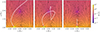Fig. 1. Magnetic configuration at initial times for cases C1, C2, and C3. The magnitude of the magnetic field is shown in colour. Magnetic field lines are represented in black, and the MFR trajectory in white. The final times of the trajectories are t ∼ 69 min, t ∼ 175 min, and t ∼ 50 min, respectively.

Based on these contrasting behaviours, we explored how evolution changes when the temperature of the MFR (T_MFR) is varied, making the MFR colder (case ${\mathrm{C}}_T^{-}$) or hotter (case ${\mathrm{C}}_T^{+}$). This temperature change affects the MFR’s weight through gas pressure equilibrium. The centres of colder MFRs are heavier (∼10 times), whereas hotter ones are lighter (∼10 times) than in the correspondent reference case C.

Next, we examined how the dynamics of the reference cases change when the background magnetic field is varied (cases ${\mathrm{C}1}_{B_{\mathrm{BKG}}}^{+}$ and ${\mathrm{C}2}_{B_{\mathrm{BKG}}}^{-}$), to evaluate the influence of the surrounding magnetic environment on the ascension process. For ${\mathrm{C}1}_{B_{\mathrm{BKG}}}^{+}$, the values of the magnetic field at the coronal base are between ∼2 − 4 G, while for ${\mathrm{C}2}_{B_{\mathrm{BKG}}}^{-}$, the values are between ∼0.5 − 1 G.

Additionally, we analysed whether changing the MFR’s own magnetic field strength alters its dynamics (case ${\mathrm{C}2}_{B_{\mathrm{MFR}}}^{+}$). To achieve an ejection, we increased the current values from (j₀, j₁) = (−126, −106) statA cm⁻² to (j₀, j₁) = (−136, −119) statA cm⁻². This adjustment increased the central magnetic field strength of the MFR from B_MFR = 38 G to B_MFR = 43 G, thereby enhancing the force acting on it. This change significantly affects the magnetic energy, given its quadratic dependence on the magnetic field.

3. Results and discussion

To identify configurations that lead to an escaping MFR, we analysed the dynamics and described the energy and the light curves of the mean flux, comparing the different cases.

3.1. Dynamic behaviour analysis

The reference cases C1, C2, and C3 were designed to analyse how the initial position of the MFR influences its dynamic. The results show distinct behaviours: in cases C2 and C3, the MFR fails to rise, as its proximity to the central region results in stronger overlying magnetic fields, which provide a greater counteracting action against its upward motion. As evolution progresses, magnetic reconnection develops locally on the MFR surface, dispersing the B_z component and the MFR material along adjacent field lines, ultimately eroding the B_ϕ component (similar to cases 5 and 4 in C25). In contrast, in case C1, although reconnection also occurs at the MFR surface when antiparallel field lines interact, the structure of the MFR remains coherent throughout its ascent (similar to case 6, also described in C25).

To explore the impact of temperature, and consequently the mass loading of the MFR, we varied its initial temperature. We analysed the initial energy content of the MFR in each case to assess the resulting energy balance. For this, we assumed a typical MFR volume of approximately 10²⁸ cm³, corresponding to a cylindrical structure with a radius of 3.75 Mm and a length of 400 Mm. In Table 2 we show the values of the magnetic ($E_{\mathrm{mag}}=\frac{B^2}{8\pi }$), thermal ($E_{\mathrm{th}}=\frac{p}{\gamma -1}$), and gravitational (E_g = ρ g y) energies, expressed per unit of this volume.

In the hotter cases, the dynamics remain similar to the reference cases: ${\mathrm{C}1}_T^{+}$ still successfully ascends, whereas C2_T⁺ and C3_T⁺ still fail to rise (see Table 1). This indicates that a modest reduction in gravitational energy alone is not sufficient to alter the outcome (see Table 2).

However, in the colder cases, ${\mathrm{C}1}_T^{-}$, and ${\mathrm{C}2}_T^{-}$, where the MFRs are heavier due to the reduced temperature, both systems fail to ascend. In these cases, the MFR collapses towards the solar surface (COL, in Table 1), triggered by gravitational and magnetic influence.

In the hotter cases, even though E_g is an order of magnitude smaller than E_mag, a successful ascent only occurs when the MFR is initially located near the HS foot. However, in the colder cases, where E_g becomes comparable to E_mag, the MFR fails to erupt regardless of its position.

Following the previous analysis, we now investigate how the ascent of the MFR is affected by varying both the background magnetic field and that of the MFR itself. This includes cases ${\mathrm{C}1}_{B_{\mathrm{BKG}}}^{+}$, ${\mathrm{C}2}_{B_{\mathrm{BKG}}}^{-}$, and ${\mathrm{C}2}_{B_{\mathrm{MFR}}}^{+}$.

We began by focusing on the successful case C1 and analysed its behaviour when the background magnetic field doubles (${\mathrm{C}1}_{B_{\mathrm{BKG}}}^{+}$). Under this stronger background, the MFR fails to ascend and disintegrates during its evolution. Conversely, in the previously unsuccessful case C2, if the background field is reduced to 0.5 G (${\mathrm{C}2}_{B_{\mathrm{BKG}}}^{-}$), the MFR’s magnetic flux becomes strong enough to overcome the confinement, enabling a successful ascent through the strapping field (see Table 1).

Next, we kept the background magnetic field unchanged and increased the magnetic flux of the MFR in case C2, which previously failed to ascend. We find that the enhanced magnetic flux (${\mathrm{C}2}_{B_{\mathrm{MFR}}}^{+}$) allows the MFR to better resist erosion while rising through the strapping field, resulting in a successful ascent.

Both phenomena are closely related to the parameter q_MFR/MC defined in C25, which characterises the ratio between the poloidal magnetic flux of the MFR and the strapping flux of the surrounding magnetic field. A higher q_MFR/MC value implies that the MFR has a stronger capacity to overcome the overlying magnetic tension. When we increase the MFR flux, the system reaches a critical q_MFR/MC value that allows the structure to resist magnetic erosion and ascend successfully.

Similarly, when we reduce the background field, the strapping flux becomes weaker, increasing q_MFR/MC to a level that allows the MFR to rise, despite previous failed under stronger confinement. Conversely, when we double the background magnetic field in the previously successful case, the increased strapping field reduces q_MFR/MC, leading the MFR to fail to ascend and to disintegrate.

These results reinforce the idea that both the internal properties of the MFR and the characteristics of the surrounding coronal environment critically affect the ascent process.

3.2. Light curve analysis

Considering that the simulated evolution of the MFR occurs in the plane of the sky of a Sun-like star, in this section we analyse the light curves of the integrated fluxes at different EUV wavelengths (304, 171, and 94 Å ), as observed by the Atmospheric Imaging Assembly (AIA; Lemen et al. 2012) on board the Solar Dynamics Observatory (SDO; Pesnell et al. 2012).

We examined the behaviour in three distinct groups: escaping cases ($\mathrm{C}1,{\mathrm{C}1}_T^{+},{\mathrm{C}2}_{B_{\mathrm{MFR}}}^{+},{\mathrm{C}2}_{B_{\mathrm{BKG}}}^{-}$), eroded cases ($\mathrm{C}2,\mathrm{C}3,{\mathrm{C}2}_T^{+},{\mathrm{C}3}_T^{+},{\mathrm{C}3}_T^{-},{\mathrm{C}1}_{B_{\mathrm{BKG}}}^{+}$), and collapsed cases (${\mathrm{C}1}_T^{-},{\mathrm{C}2}_T^{-}$). We selected cases C1, C2, and ${\mathrm{C}2}_T^{-}$ as representatives of each group, respectively. Since all channels exhibit similar behaviour, Fig. 2 shows the evolution of the synthetic 304 Å images for each representative case in separate rows.

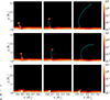Fig. 2. Synthetic 304 Å images showing the temporal evolution of cases C1 (first row), C2 (second row), and C2T− (third row) at times 13 min (first column), 22 min (second column) and 56 min (third column). The MFR trajectory is superimposed in cyan. Associated movies in 304 and 171 Å are available online.

The initial values of the synthesised EUV images of the flux ropes differ between these cases. In cases C1 and C2, where the MFR temperature is initially 1 MK, the flux rope appears brighter than the coronal background in all three channels. Meanwhile, in case C2_T⁻, where the MFR temperature is 0.1 MK, the flux rope appears darker in the hotter EUV channels (94 and 171 Å).

For each group, we present the light curves in Fig. 3. These were obtained by computing the difference between the integrated flux of case C within the simulated domain (F_C(t)) and the background flux without the flux rope (F_BKG(t)) over time.

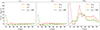Fig. 3. Integrated fluxes for representative cases of successful escape (C1), eroded (C2) and collapsed (${\mathrm{C}2}_T^{-}$) MFRs.

Cases C1 and C2 exhibit similar behaviour. Initially, both cases show an enhancement relative to the background because the MFR temperature is the same as that of its surroundings but with a higher density, which makes it brighter at the beginning. As the MFR rises and either is ejected or becomes eroded, the emission decreases and remains low because its interaction with the surrounding plasma occurs at increasing heights where the coronal density drops, which prevents the formation of pronounced emission peaks (see the evolution of these cases in the upper and middle panels of Fig. 2). Although case C2 shows a slight increase in 304 Å, this enhancement is not significant.

In contrast, case C2_T⁻ presents a different behaviour. At the initial time, the coolest channel shows a significant enhancement with respect to the background, since under the initial conditions the MFR temperature lies near the peak of the AIA response function and its density is one order of magnitude higher than that of the MFRs in cases C1 and C2. In contrast, in the hotter channels, the MFR temperature remains below the peak of the corresponding AIA response functions. Subsequently, the emission in the 304 Å channel decreases. However, when the MFR begins to fall back towards the chromosphere from 12 min onwards, it interacts with the low corona and the upper chromosphere, producing an enhancement in the emission at this wavelength (see the bottom panel of Fig. 2 and its corresponding animation). We observe a similar effect in the hotter 171 Å channel and also in 94 Å; however, in the latter case the amplitude is two orders of magnitude smaller.

Another notable feature is that the sharp increase in 304 Å emission begins at ∼12 min, when the MFR falls back and interacts with the low corona. In the hotter channels, this increase occurs later, at 25 min, when the MFR impacts the upper chromosphere (see the animation of 171 Å).

While the initial conditions set the evolution of the MFR, the observed emission is ultimately governed by the flux rope dynamics and its interaction with the surroundings.

3.3. Velocity analysis

We now consider the evolution of the velocity for different cases representing escape of the MFR (C1), confinement in the form of erosion (C2) or collapse (${\mathrm{C}2}_T^{-}$). For this, we performed two complementary calculations. First, we calculated the vertical velocity of the plasma (v_y) in our entire simulation box (see Fig. 4). This calculation allows us to evaluate the response of the velocity structure of the MFR and the corona as the events develop. The upper left and middle panels of the figure show that the behaviour of a successful and an eroded CME (respectively) is initially similar. However, as they evolve (corresponding bottom panels), they diverge: the MFR and the surroundings exhibit a net upward velocity in the former case and a net downward motion in the latter. In contrast, the case in which the MFR collapses (right upper and bottom panels) exhibits a small displacement of the plasma. This suggests that if the CME’s direction of motion aligns with the line of sight or is at an angle that allows for a meaningful plasma Doppler velocity measurement, it is possible to discriminate between the two first scenarios.

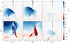Fig. 4. Plasma vertical velocity (vy) for the simulated cases, comparing a successful CME (C1, left), eroded CME (C2, middle), and collapsed CME (C2T−, right). Upper panels: Snapshots taken at a fixed time (t = 19 min). Bottom panels: Instances that maximise the contrast in the integrated bulk velocity of the MFR for each case (C1: t = 50 min, C2: t = 75 min, and C2T−: t = 25 min; see Fig. 5). In all panels, the heliospheric current sheet formed along the x = 0 position is visible at heights above y = 2 R⊙.

To estimate how much MFR motion contributes to the Doppler effect, we computed the average vertical velocity inside the MFR (${\overline{v}}_y$), weighted by the normalised area (A): ${\widehat{v}}_y(t)={\overline{v}}_y(t)A(t)/A(0)$ (see Fig. 5). The area is defined as that enclosed by closed magnetic field lines. We calculated the values of the MFR centre velocity, v_y, MFR, for all cases. The escape case is distinguishable from the eroded and collapsed (failed) cases by its behaviour. The escape curve ${\widehat{v}}_y(t)$ has larger value at all times than the failed ones. In contrast to the failed cases, where the curves tend to zero at the final stages, the escape curve ends with a non-vanishing value. The escape curve reaches a much larger altitude than the failed ones, which end at lower heights. The velocity curves v_y, MFR show that the escape case has large values throughout the evolution, the collapsed case has relatively small velocity values at all times, and the eroded case corresponds to the MFR that rebounds at relatively small altitudes.

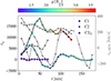Fig. 5. Left vertical axis: Evolution of the average vertical velocity inside the MFR, weighted by normalised area ${\widehat{v}}_y$ (black lines). Squares, circles, and diamonds represent cases C1, C2, and ${\mathrm{C}2}_T^{-}$, respectively. Symbol colours indicate the height of the MFR centre. Right vertical axis: MFR centre velocity values vy, MFR (grey lines).

4. Conclusions

In this study, we investigated how the likelihood of CME escape depends not only on the strength of the large-scale magnetic field, but also on local conditions, including the position of the MFR relative to the legs of the overlying HS, its mass (or equivalently, its temperature), and its internal magnetic field strength.

To this end, we adopted an MFR catastrophe model, a configuration that has not yet been applied in global stellar simulations, where the Gibson & Low (1998) and Titov & Démoulin (1999) models are typically used. This choice is significant, as it shows that our results remain qualitatively consistent even when using a different numerical code and a different MFR model. With this approach, we investigated a range of scenarios in which the MFR either successfully erupts or fails to rise. Among the failed cases, we identify two distinct behaviours. The first involves MFR disintegration through magnetic reconnection during its evolution, which causes the structure to lose its identity as its plasma merges into the surrounding medium. The second occurs when the MFR, unable to sustain its ascent, collapses under its own weight and falls back to the chromosphere –a behaviour characteristic of “heavy” MFRs (those with relatively low temperatures). This leads to a threefold classification: MFRs that escape successfully, those that are confined by erosion, and those that fail by collapse.

We also analysed how changes in the magnetic field affect the dynamics. By varying the magnetic flux of the MFR –that is, increasing or decreasing the axial and poloidal current densities – the Lorentz force correspondingly strengthens or weakens, which enhances or reduces the MFR’s ability to ascend, respectively.

Conversely, when considering a weaker or stronger background magnetic field, the confinement provided by the strapping field decreases or increases, respectively. Hence, a lower or higher strength of the large-scale magnetic field implies a higher or lower capability of the MFR to rise. Thus, as shown by Cécere et al. (2025), the relation between the MFR’s poloidal magnetic flux and the strapping flux of the surrounding magnetic field serves as a quantitative measure of the MFR’s likelihood of ejection.

This indicates that Sun-like stars with stronger magnetic fields do not necessarily experience more frequent ejections because the initial magnetic flux of the MFR plays a crucial role. Additionally, we suggest that the ejection also depends on factors such as the mass of the MFR and its position relative to the large-scale magnetic structure.

Inspired by Alvarado-Gómez et al. (2019), we analysed how these MFR evolutions would appear in the EUV for Sun-like stars. We find that the light curve fluxes exhibit a peak in emission only in cases where the ascent fails by collapse. From a photometric observation standpoint, we can only clearly distinguish the cases in which collapse occurs. Thus, photometric measurements alone do not allow us to differentiate whether the MFR disintegrates or successfully ascends. Detectable observational signatures are generated only when the MFR impacts the chromosphere.

We also conducted Doppler shift estimations to determine whether these measurements could serve as discriminators between MFR disintegration and successful ascension events. Our analysis suggests that if the CME’s direction of motion aligns with the line of sight or is at an angle that allows for a meaningful Doppler velocity measurement, it is possible to discriminate between the escape case and the eroded one.

Our restricted and qualitative parametric study suggests the following:

1. Stronger global background magnetic fields lead to more confining magnetic cages, which can prevent or even erode the MFR before it escapes.

2. Whether a flux rope is eroded or falls back depends primarily on the balance between magnetic and gravitational energy.

3. Photometrically, successfully ejected CMEs do not exhibit prominent EUV emission peaks.

4. When considering narrow-band EUV filters, collapsed events may be misidentified as flares in observations.

5. Doppler analysis could eventually allow us to discern between an escape scenario and an eroded one.

These results indicate that in Sun-like stars, the same conditions that increase magnetic energy also enhance magnetic confinement effects, potentially suppressing CME escape and altering their observational signatures.

A more extensive parameter study, involving a significantly larger number of simulations, would provide a stronger basis for the conclusions and help assess the sensitivity of the results to variations in the input parameters. Such a systematic exploration is part of our planned future work.

Data availability

Movies associated to Fig. 2 are available at https://www.aanda.org

Acknowledgments

MC and AC are members of the Carrera del Investigador Científico (CONICET). They acknowledge support from the DynaSun project, which has received funding under the Horizon Europe programme of the European Union, grant agreement no. 101131534. Views and opinions expressed are however those of the author only and do not necessarily reflect those of the European Union and therefore the European Union cannot be held responsible for them. Further support was provided by SeCyT under grant number 33820230100116CB. Also, we thank the Centro de Cómputo de Alto Desempeño (UNC), where the simulations were performed. The software used in this work was developed in part by the DOE NNSA- and DOE Office of Science-supported Flash Center for Computational Science at the University of Chicago and the University of Rochester. The authors thank the referee for all the suggestions and comments, which have constructively helped to improve and strengthen the manuscript.

References

Appendix A: Model

A.1. Ideal MHD equations

The ideal MHD equations for a stratified medium, in CGS units and in conservative form, are:

$$\begin{array}{c}\hfill \frac{\partial \rho }{\partial t}+\mathrm{\nabla }·(\rho \mathit{v})=0,\end{array}$$(A.1)

$$\begin{array}{c}\hfill \frac{\partial (\rho \mathit{v})}{\partial t}+\mathrm{\nabla }·(\rho \mathit{v}\mathit{v}-\frac{1}{4\pi }\mathit{B}\mathit{B})+\mathrm{\nabla }p+\mathrm{\nabla }\left(\frac{B^2}{8\pi }\right)=\rho \mathit{g},\end{array}$$(A.2)

$$\begin{array}{c}\hfill \frac{\partial E}{\partial t}+\mathrm{\nabla }·[(E+p+\frac{B^2}{8\pi })\mathit{v}-\frac{1}{4\pi }\left(\mathit{v}·\mathit{B}\right)\mathit{B}]=\rho \mathit{g}·\mathit{v},\end{array}$$(A.3)

$$\begin{array}{c}\hfill \frac{\partial \mathit{B}}{\partial t}+\mathrm{\nabla }·(\mathit{v}\mathit{B}-\mathit{B}\mathit{v})=\mathit{0},\end{array}$$(A.4)

where ρ denotes the plasma density, v the velocity, B the magnetic field, p the gas pressure, and g the gravitational acceleration. The total energy per unit volume, E, is defined as

$$\begin{array}{c}\hfill E=\rho ϵ+\frac{1}{2}\rho v^2+\frac{B^2}{8\pi },\end{array}$$

with ϵ being the specific internal energy. In this formulation, the current density is given by $\mathit{j}=\frac{c}{4\pi }\mathrm{\nabla }\times \mathit{B}$ (with c being the speed of light), and the solenoidal condition $\mathrm{\nabla }·\mathit{B}=0$ holds for the magnetic field. We assume the plasma is fully ionised hydrogen obeying the ideal gas law, p = ρRT/μ = (γ − 1)ρϵ, where, R is the gas constant, T is the temperature, μ is the molar mass, and γ is the specific heat ratio, taken as 5/3.

A.2. Magnetic field configuration

The initial out-of-equilibrium magnetic configuration for the MFR is given by:

$$\begin{array}{cc}\hfill B_{x,\mathrm{MFR}}=& B_{\varphi }(R_{-})\frac{(y-h_0)}{R_{-}}-B_{\varphi }(R_{+})\frac{(y+h_0)}{R_{+}}\hfill \\ \hfill & -Md{B}_{\varphi }(r+\frac{\mathrm{\Delta }}{2})(r+\frac{\mathrm{\Delta }}{2})\frac{{(x-x_{\mathrm{MFR}})}^2-{(y+d)}^2}{R_d^4},\hfill \\ \hfill B_{y,\mathrm{MFR}}=& -B_{\varphi }(R_{-})\frac{x-x_{\mathrm{MFR}}}{R_{-}}+B_{\varphi }(R_{+})\frac{x-x_{\mathrm{MFR}}}{R_{+}}\hfill \\ \hfill & -Md{B}_{\varphi }(r+\frac{\mathrm{\Delta }}{2})(r+\frac{\mathrm{\Delta }}{2})\frac{2(x-x_{\mathrm{MFR}})(y+d)}{R_d^4},\hfill \\ \hfill B_{z,\mathrm{MFR}}=& B_{\text{z}}(R_{-}).\hfill \end{array}$$(A.5)

Here, h₀ denotes the initial height of the MFR, x_MFR its position along the x-axis, and M the strength of the line dipole located at a depth d. The radius of the current-carrying wire is r, and Δ represents the thickness of the transition layer between the wire and the surrounding medium. The distances measured from different reference points are defined as follows: $R_{-}=\sqrt{{(x-x_{\mathrm{MFR}})}^2+{(y-h_0)}^2}$ (current), $R_{+}=\sqrt{{(x-x_{\mathrm{MFR}})}^2+{(y+h_0)}^2}$ (image current), and $R_d=\sqrt{{(x-x_{\mathrm{MFR}})}^2+{(y+d)}^2}$ (dipole). Finally, B_ϕ denotes the poloidal magnetic field generated by the current density in the wire:

$$\begin{array}{c}\hfill B_{\varphi }(R)=\{\begin{array}{cc}{\displaystyle -\frac{2\pi }{c}{j}_{0}R,}\hfill & 0\le R<r-\frac{\mathrm{\Delta }}{2},\hfill \\ {\displaystyle -\frac{2\pi j_0}{\mathit{cR}}(\frac{1}{2}{(r-\frac{\mathrm{\Delta }}{2})}^2-{\left(\frac{\mathrm{\Delta }}{\pi }\right)}^2+}\hfill \\ \frac{R^2}{2}+\frac{\mathrm{\Delta }R}{\pi }sin\left[\frac{\pi }{\mathrm{\Delta }}(R-r+\frac{\mathrm{\Delta }}{2})\right]+\hfill \\ {\left(\frac{\mathrm{\Delta }}{\pi }\right)}^{2}cos\left[\frac{\pi }{\mathrm{\Delta }}(R-r+\frac{\mathrm{\Delta }}{2})\right])\hfill & r-\frac{\mathrm{\Delta }}{2}\le R<r+\frac{\mathrm{\Delta }}{2},\hfill \\ {\displaystyle -\frac{2\pi j_0}{\mathit{cR}}[r^2+{\left(\frac{\mathrm{\Delta }}{2}\right)}^2-2{\left(\frac{\mathrm{\Delta }}{\pi }\right)}^2],}\hfill & R\ge r+\frac{\mathrm{\Delta }}{2},\hfill \end{array}\end{array}$$(A.6)

and

$$\begin{array}{c}\hfill j_z(R)=\{\begin{array}{c}\hfill \begin{array}{cccc}& j_0\hfill & \hfill & 0\le R<r-\frac{\mathrm{\Delta }}{2}\\ \hfill & \frac{j_0}{2}\{cos\left[\frac{\pi }{\mathrm{\Delta }}(R-r+\frac{\mathrm{\Delta }}{2})\right]+1\}\hfill & \hfill & r-\frac{\mathrm{\Delta }}{2}\le R<r+\frac{\mathrm{\Delta }}{2}\\ \hfill & 0\hfill & \hfill & \mathrm{R}\ge r+\frac{\mathrm{\Delta }}{2},\end{array}\end{array}\end{array}$$(A.7)

respectively.

$$\begin{array}{cc}\hfill j_{\varphi }(R)=j_{1}R{\left[\sqrt{{(r-\frac{\mathrm{\Delta }}{2})}^2-R^2}\right]}^{-1}& 0\le R<r-\frac{\mathrm{\Delta }}{2}\hfill \end{array}$$(A.8)

$$\begin{array}{cc}\hfill B_{\mathrm{z}}(R)=\frac{4\pi j_1}{c}\sqrt{{(r-\frac{\mathrm{\Delta }}{2})}^2-R^2}& 0\le R<r-\frac{\mathrm{\Delta }}{2},\hfill \end{array}$$(A.9)

where j₁ is the intensity of the current density.

As the background configuration, we select an HS magnetic field with x- and y-components.

$$\begin{array}{c}\hfill B_{x,\mathrm{HS}}-i{B}_{y,\mathrm{HS}}=B_0\frac{{(\omega +i{y}_N)}^{1/2}\omega -i{y}_N{)}^{1/2}}{F(a,b,y_N)}ln\left(\frac{{\omega }^2-a^2}{{\omega }^2-b^2}\right)\end{array}$$(A.10)

with B₀ the strength of the magnetic field, ω = x + i y, a ∼ 0.26 R_⊙, b ∼ 0.79 R_⊙, y_N = 1.9 R_⊙, and

$$\begin{array}{c}\hfill \begin{array}{cc}\hfill F(a,b,y_N)=& \frac{1}{2(b-a)}[b{(b^2+y_N^2)}^{1/2}-a{(a^2+y_N^2)}^{1/2}\hfill \\ \hfill & +y_N^{2}ln\left(\frac{b+{(b^2+y_N^2)}^{1/2}}{a+{(a^2+y_N^2)}^{1/2}}\right)].\hfill \end{array}\end{array}$$

The total magnetic field results from the combination of both magnetic structures:

$$\begin{array}{cc}\hfill B_x& =B_{x,\mathrm{MFR}}+B_{x,\mathrm{HS}},\hfill \\ \hfill B_y& =B_{y,\mathrm{MFR}}+B_{y,\mathrm{HS}},\hfill \\ \hfill B_z& =B_{z,\mathrm{MFR}}.\hfill \end{array}$$(A.11)

A.3. Thermodynamic variables

For a stratified solar atmosphere, the pressure profile is defined as:

$$\begin{array}{c}\hfill p(y)=\{\begin{array}{c}\hfill \begin{array}{cccc}& p_{\mathrm{ch}}exp\left[\frac{\alpha }{T_{\mathrm{ch}}}(\frac{1}{h_{\mathrm{ch}}+R_{\odot }}-\frac{1}{y+R_{\odot }})\right]\hfill & \hfill & 0\le y<h_{\mathrm{ch}}\\ \hfill & p_{\mathrm{ch}}exp[-{\displaystyle {\int }_{h_{\mathrm{ch}}}^y}\frac{\alpha }{T(y^{\prime })}{(R_{\odot }+y^{\prime })}^{-2}d{y}^{\prime }]\hfill & \hfill & h_{\mathrm{ch}}\le y<h_{\mathrm{c}}\\ \hfill & n_{\mathrm{c}}{k}_B{T}_{\mathrm{c}}exp\left[\frac{\alpha }{T_{\mathrm{c}}}(\frac{1}{y+R_{\odot }}-\frac{1}{h_{\mathrm{c}}+R_{\odot }})\right]\hfill & \hfill & h_{\mathrm{c}}\le y,\end{array}\end{array}\end{array}$$(A.12)

where the gravitational acceleration is defined as $\mathit{g}=-\frac{G{M}_{\odot }}{{(y+R_{\odot })}^2}{\mathit{e}}_y$, with G denoting the gravitational constant, M_⊙ the solar mass, and R_⊙ the solar radius, and $\alpha =\frac{G{M}_{\odot }\mu }{R_{\mathrm{gas}}}$. Also,

$$\begin{array}{c}\hfill p_{\mathrm{ch}}=n_{\mathrm{c}}{k}_B{T}_{\mathrm{c}}exp\left[{\displaystyle {\int }_{h_{\mathrm{ch}}}^{h_{\mathrm{c}}}}\frac{\alpha }{T(y^{\prime })}{(R_{\odot }+y^{\prime })}^{-2}d{y}^{\prime }\right],\end{array}$$(A.13)

where n_c is the number density at height y = h_c.

The initial internal pressure of the MFR is derived from an approximate equilibrium solution:

$$\begin{array}{cc}\hfill p_{\mathrm{MFR}}(x,y)=p(y)& +\frac{1}{c}{\displaystyle {\int }_R^{r+\frac{\mathrm{\Delta }}{2}}}{B}_{\varphi }(R^{\prime })j_z(R^{\prime })d{R}^{\prime }\hfill \\ \hfill & -\frac{1}{c}{\displaystyle {\int }_R^{r+\frac{\mathrm{\Delta }}{2}}}{B}_{\text{z}}(R^{\prime })j_{\varphi }(R^{\prime })d{R}^{\prime }.\hfill \end{array}$$(A.14)

The resulting plasma densities are determined based on the adopted equation of state, i.e.:

$$\begin{array}{c}\hfill {\rho }_{\mathrm{MFR}}=\frac{p_{\mathrm{MFR}}\mu }{RT(y)}.\end{array}$$(A.15)

All Tables

All Figures

	Fig. 1. Magnetic configuration at initial times for cases C1, C2, and C3. The magnitude of the magnetic field is shown in colour. Magnetic field lines are represented in black, and the MFR trajectory in white. The final times of the trajectories are t ∼ 69 min, t ∼ 175 min, and t ∼ 50 min, respectively.
In the text

	Fig. 2. Synthetic 304 Å images showing the temporal evolution of cases C1 (first row), C2 (second row), and C2T− (third row) at times 13 min (first column), 22 min (second column) and 56 min (third column). The MFR trajectory is superimposed in cyan. Associated movies in 304 and 171 Å are available online.
In the text

	Fig. 3. Integrated fluxes for representative cases of successful escape (C1), eroded (C2) and collapsed (${\mathrm{C}2}_T^{-}$) MFRs.
In the text

Fig. 4. Plasma vertical velocity (vy) for the simulated cases, comparing a successful CME (C1, left), eroded CME (C2, middle), and collapsed CME (C2T−, right). Upper panels: Snapshots taken at a fixed time (t = 19 min). Bottom panels: Instances that maximise the contrast in the integrated bulk velocity of the MFR for each case (C1: t = 50 min, C2: t = 75 min, and C2T−: t = 25 min; see Fig. 5). In all panels, the heliospheric current sheet formed along the x = 0 position is visible at heights above y = 2 R⊙.

In the text

	Fig. 5. Left vertical axis: Evolution of the average vertical velocity inside the MFR, weighted by normalised area ${\widehat{v}}_y$ (black lines). Squares, circles, and diamonds represent cases C1, C2, and ${\mathrm{C}2}_T^{-}$, respectively. Symbol colours indicate the height of the MFR centre. Right vertical axis: MFR centre velocity values vy, MFR (grey lines).
In the text

References

- Alvarado-Gómez, J. D., Drake, J. J., Cohen, O., Moschou, S. P., & Garraffo, C. 2018, ApJ, 862, 93 [Google Scholar]
- Alvarado-Gómez, J. D., Drake, J. J., Moschou, S. P., et al. 2019, ApJ, 884, L13 [CrossRef] [Google Scholar]
- Alvarado-Gómez, J. D., Drake, J. J., Fraschetti, F., et al. 2020, ApJ, 895, 47 [Google Scholar]
- Alvarado-Gómez, J. D., Drake, J. J., Cohen, O., et al. 2022, Astron. Nachr., 343, e10100 [Google Scholar]
- Argiroffi, C., Reale, F., Drake, J. J., et al. 2019, Nat. Astron., 3, 742 [NASA ADS] [CrossRef] [Google Scholar]
- Benz, A. O. 2017, Liv. Rev. Sol. Phys., 14, 2 [Google Scholar]
- Cécere, M., Wyper, P. F., Krause, G., Sahade, A., & Rice, O. E. K. 2025, A&A, 697, A155 [NASA ADS] [CrossRef] [EDP Sciences] [Google Scholar]
- Drake, J. J., Cohen, O., Yashiro, S., & Gopalswamy, N. 2013, ApJ, 764, 170 [NASA ADS] [CrossRef] [Google Scholar]
- Drake, J. J., Cohen, O., Garraffo, C., & Kashyap, V. 2016, IAU Symp., 320, 196 [NASA ADS] [Google Scholar]
- Forbes, T. G. 1990, J. Geophys. Res., 95, 11919 [NASA ADS] [CrossRef] [Google Scholar]
- Fryxell, B., Olson, K., Ricker, P., et al. 2000, ApJS, 131, 273 [Google Scholar]
- Gibson, S. E., & Low, B. C. 1998, ApJ, 493, 460 [NASA ADS] [CrossRef] [Google Scholar]
- Gopalswamy, N., Michałek, G., Yashiro, S., et al. 2024, ArXiv e-prints [arXiv:2407.04165] [Google Scholar]
- Hu, Y. Q. 2001, Sol. Phys., 200, 115 [Google Scholar]
- Kochukhov, O. 2021, A&ARv, 29, 1 [Google Scholar]
- Kowalski, A. F. 2024, Liv. Rev. Sol. Phys., 21, 1 [NASA ADS] [CrossRef] [Google Scholar]
- Lamy, P. L., Floyd, O., Boclet, B., et al. 2019, Space Sci. Rev., 215, 39 [CrossRef] [Google Scholar]
- Leitzinger, M., & Odert, P. 2022, Serb. Astron. J., 205, 1 [NASA ADS] [CrossRef] [Google Scholar]
- Lemen, J. R., Title, A. M., Akin, D. J., et al. 2012, Sol. Phys., 275, 17 [Google Scholar]
- Liu, L., Wang, Y., Wang, J., et al. 2016, ApJ, 826, 119 [NASA ADS] [CrossRef] [Google Scholar]
- Moschou, S.-P., Drake, J. J., Cohen, O., et al. 2019, ApJ, 877, 105 [NASA ADS] [CrossRef] [Google Scholar]
- Mullan, D. J., & Paudel, R. R. 2019, ApJ, 873, 1 [NASA ADS] [CrossRef] [Google Scholar]
- Namekata, K., Maehara, H., Honda, S., et al. 2021, Nat. Astron., 6, 241 [Google Scholar]
- Pariat, E., Wyper, P. F., & Linan, L. 2023, A&A, 669, A33 [NASA ADS] [CrossRef] [EDP Sciences] [Google Scholar]
- Pesnell, W. D., Thompson, B. J., & Chamberlin, P. C. 2012, Sol. Phys., 275, 3 [Google Scholar]
- Sahade, A., Cécere, M., Sieyra, M. V., et al. 2022, A&A, 662, A113 [NASA ADS] [CrossRef] [EDP Sciences] [Google Scholar]
- Sahade, A., Vourlidas, A., Balmaceda, L. A., & Cécere, M. 2023, ApJ, 953, 150 [Google Scholar]
- Sun, X., Bobra, M. G., Hoeksema, J. T., et al. 2015, ApJ, 804, L28 [Google Scholar]
- Titov, V. S., & Démoulin, P. 1999, A&A, 351, 707 [NASA ADS] [Google Scholar]
- Veronig, A. M., Odert, P., Leitzinger, M., et al. 2021, Nat. Astron., 5, 697 [NASA ADS] [CrossRef] [Google Scholar]
- Webb, D. F., & Howard, T. A. 2012, Liv. Rev. Sol. Phys., 9, 3 [Google Scholar]
- Xu, Y., Tian, H., Alvarado-Gómez, J. D., Drake, J. J., & Guerrero, G. 2025, ApJ, 985, 219 [Google Scholar]