| Issue |
A&A
Volume 697, May 2025
|
|
|---|---|---|
| Article Number | A155 | |
| Number of page(s) | 10 | |
| Section | The Sun and the Heliosphere | |
| DOI | https://doi.org/10.1051/0004-6361/202450239 | |
| Published online | 14 May 2025 | |
Helmet streamer influence on the evolution of magnetic flux ropes
1
Instituto de Astronomía Teórica y Experimental, CONICET-UNC, Córdoba, Argentina
2
Observatorio Astronómico de Córdoba, UNC, Córdoba, Argentina
3
Department of Mathematical Sciences, Durham University, Durham DH1 3LE, UK
4
Instituto de Estudios Avanzados en Ingeniería y Tecnología, CONICET-UNC, Córdoba, Argentina
5
NASA Goddard Space Flight Center, Greenbelt, MD 20771, USA
⋆ Corresponding author: mariana.cecere@unc.edu.ar
Received:
4
April
2024
Accepted:
20
March
2025
Context. Solar eruptions play a major role in space weather. Understanding the physical mechanisms that influence their evolution is essential for improving future predictions about the geo-effectiveness of an event. Helmet streamers (HSs) are present in the solar corona during both periods of minimum and maximum solar activity. This magnetic structure features a current sheet of low magnetic energy, towards which coronal mass ejection events tend to deflect. However, there is also a closed magnetic field region underlying this current sheet where eruptions are often confined. This makes it an interesting structure to study, as the inherent complexity of the structure hinders the predictability of the eruption.
Aims. The aim of this study is to investigate the influence of the HS on the evolution and potential confinement of a magnetic flux rope (MFR). We explore magnetic configurations involving the MFR and HS that are more likely to allow the MFR to rise through the overlying magnetic field, with the ultimate goal of establishing simple parameters that can help predict the conditions under which an MFR can ascend or remain confined.
Methods. Through 2.5D magnetohydrodynamic numerical simulations, we emulated the dynamics of MFRs in the presence of an HS. We analysed the dynamics of different magnetic field configurations, paying special attention to the mechanisms that facilitate the ascent or confinement of the MFR.
Results. We find that the null point reconnection mechanism plays a fundamental role in the dynamics of the MFR. Depending on the initial configuration, null point reconnection can either confine the ascent by disrupting the MFR or facilitate its rise by reducing the strapping flux above it. We also identify a critical value in the relationship between the magnetic flux that the MFR must traverse during its ascent and its own magnetic flux. We find that if the strapping flux above the MFR is less than two-thirds of its own poloidal flux, the MFR is able to ascend.
Conclusions. In our simulations, null point reconnection plays a major role in facilitating the ascent of the MFR. A key factor in predicting whether the MFR will rise is the initial ratio between its poloidal flux and the strapping magnetic flux above it.
Key words: magnetohydrodynamics (MHD) / methods: numerical / Sun: coronal mass ejections (CMEs) / Sun: magnetic fields
© The Authors 2025
 Open Access article, published by EDP Sciences, under the terms of the Creative Commons Attribution License (https://creativecommons.org/licenses/by/4.0), which permits unrestricted use, distribution, and reproduction in any medium, provided the original work is properly cited.
This article is published in open access under the Subscribe to Open model. Subscribe to A&A to support open access publication.
1. Introduction
Coronal mass ejections (CMEs) play a crucial role in space weather forecasting, and predicting their occurrence requires understanding not only the trajectories but also the likelihood of an event. In this context, several studies have analysed the physical nature of magnetic flux rope (MFR) eruptions through the study of magnetic fluxes. For example, Zhang et al. (2020) demonstrate that an increase in magnetic flux, primarily axial, within the MFR drives the rope to evolve towards a critical condition, eventually triggering its eruption at a certain threshold. On the other hand, using the catastrophe model, Forbes (2000) showed that while ejection is related to an increase in magnetic flux, a decrease can also lead to ejection (Zhuang et al. 2018).
Other studies emphasise the crucial role of the ambient environment in determining ejection outcomes. In the context of flux rope eruptions, Rice & Yeates (2023) show that there exists a clear threshold in ratios between the magnetic flux in a flux rope and various quantities influenced by the strength of the background field, above which an eruption is very likely. They also tested the predictability of these eruptions against measures such as the eruptivity index (Pariat et al. 2017), finding that the large peaks originally observed in the eruptivity index prior to eruptions were due to the orientation of the ambient magnetic field. In the context of pseudo-streamer eruptions, Talpeanu et al. (2022) demonstrate that neighbouring magnetic structures can decelerate the eruption through magnetic reconnection, creating overlapping arcs that increase confinement. Moreover, this interchange (open-closed) reconnection leads to the opening of a considerable fraction of the MFR flux, partially altering the MFR’s path and affecting the CME deflection (Ben-Nun et al. 2023).
Masson et al. (2013) demonstrated that, in a null point configuration beneath a helmet streamer (HS), when the amount of overlying closed flux is small compared to the erupting flux, such as when a coronal hole is near the eruption, interchange reconnection is likely. Conversely, if the amount of overlying closed flux is large, interchange reconnection becomes highly unlikely. Similar findings were reported in Sahade et al. (2022), who simulated an eruption occurring inside a pseudo-streamer structure. This study revealed that significant overlying magnetic cage (MC) flux quantities act as a preventive factor, hindering an eruption. Similarly, Karpen et al. (2024) report on an observed confined eruption within a pseudo-streamer, comparing it to a 3D simulation, also finding that significant overlying flux plays an important role.
The goal of this paper is to analyse the evolution of MFR fluxes through their interaction with the surrounding magnetic field fluxes. While this study focuses on understanding the factors that influence the ascent and confinement of MFRs, the ultimate objective is to contribute to future efforts in predicting their potential eruptivity. We assumed an unstable MFR superimposed with an HS structure (Sect. 2). Null point reconnection can play either a stabilising or a destabilising role in the evolution depending upon the configuration. We show that in some cases the flux rope is destroyed or reaches a new equilibrium. In these stable cases, there is significant overlying flux that also acts to suppress the eruption (Sect. 3). We demonstrate that overlying flux erosion by null point reconnection plays a key role in achieving a successful ascent (in the manner of Masson et al. 2013), with the caveat that there is no solar wind in our simulation. However, the direction of this reconnection is key, and the opposite scenario of the flux rope tunnelling deeper into the closed field can also occur. We discuss our results and outline our conclusions in Sect. 4.
2. Model
To study the evolution of an MFR embedded in an HS background, we numerically solved the 2.5D ideal magnetohydrodynamic equations, taking a stratified atmosphere into account. The equations in their Cartesian conservative form with CGS units are expressed as follows:
![$$ \begin{aligned} \frac{\partial E}{\partial t} + \nabla \cdot \left[\left(E + p + \frac{B^2}{8\pi }\right)\boldsymbol{v} -\frac{1}{4\pi } \left(\boldsymbol{v\cdot B}\right)\boldsymbol{B}\right] = \rho \boldsymbol{g}\cdot \boldsymbol{v} , \end{aligned} $$](/articles/aa/full_html/2025/05/aa50239-24/aa50239-24-eq3.gif)
where ρ represents the plasma density, p the gas pressure, v the velocity, B the magnetic field, and g the acceleration due to gravity. E is the total energy (per unit volume), given by
where ϵ is the internal energy. In this system, the current density is  (with c being the speed of light) and the magnetic field must satisfy the divergence-free condition ∇ ⋅ B = 0. We considered a fully ionised hydrogen plasma as the medium, where the perfect gas law applies: p = ρRT/μ = (γ − 1)ρϵ. Here, R represents the gas constant, T is the plasma temperature, μ stands for molar mass, and γ is the specific heat ratio, equal to 5/3.
We performed simulations using the FLASH code (Fryxell et al. 2000), specifically the fourth version, which is equipped with the un-split staggered mesh solver. This solver employs a second-order directionally un-split scheme with a monotonic upstream-centered scheme for conservation laws-type reconstruction and a constrained-transport method to satisfy the divergence-free condition of the magnetic field (Lee & Deane 2009). We used an atmosphere that includes a thin chromosphere to avoid cavitation effects brought on by the rapid expansion of the flux ropes in our simulations. As a consequence of the presence of the chromosphere, a strong stratification is produced at the base of the atmosphere. In this region the thermodynamic variables change by two orders of magnitude over a relatively short distance, which is covered by a few grid cells even when the maximum refinement level is used. This condition together with the need to perform long time simulations cause MUSCL methods with conventional reconstruction schemes to fail due to the emergence of spurious momentum fluxes in the gravity direction that artificially perturb the background hydrostatic equilibrium. For this reason, we implemented the well-balanced scheme proposed by Krause (2019), which uses a hydrostatic reconstruction scheme to ensure the numerical equilibrium for constant and linear temperature distributions in equilibrium atmospheres. Regarding the boundary conditions, we proceeded as follows: at the lateral boundaries, we applied an outflow condition for thermodynamic variables and a linear extrapolation for the magnetic fields to maintain the initial force-free configuration. For the upper and lower boundaries, we implemented a hydrostatic condition with constant temperature extrapolation (Krause 2019), and at the lower boundary, we also adopted a line-tied condition. Neglecting magnetic resistivity, we opted for the ideal magnetohydrodynamic equations, capitalising on the numerical diffusion in the simulations for the required dissipation, as detailed in Krause et al. (2018). The simulation’s highest resolution corresponds to cells of approximately [0.8 × 0.8] Mm2 within a physical domain of [ − 2000, 2000] Mm × [0, 8000] Mm, where the pressure and temperature gradients satisfied the refinement criterion. This simplification significantly diminished computational costs.
2.1. Magnetic field configurations
We adopted the catastrophe model by Forbes (1990) as the fundamental structure for the MFR in the simulation. In this scenario, an out-of-equilibrium magnetic configuration leading to the ascent of a MFR is established when a current-carrying wire, its image, and a magnetic dipole are present. We also introduced a current distribution solely in the ϕ direction within the MFR to generate a helical magnetic field and lower the equilibrium gas pressure. This allows us to express the magnetic field of the MFR as follows:
Here, h0 represents the initial height of the MFR, xMFR its position in x-axis, M is the strength of the line dipole at depth d, r is the radius of the current wire, Δ denotes the thickness of the transition layer between the current wire and the exterior. Additionally,  and
and  correspond to the distances measured from distinct reference points, specifically the image (+) and current (−) wire for R±, and the dipole for Rd. Also, in terms of j0, the current density of the current wire, the ϕ-component of the magnetic field is
![$$ \begin{aligned} B_\phi {(R)}\!=\! \left\{ \begin{array}{rl} \begin{alignedat}{2}&\tfrac{2\pi }{c}j_0R&\,&0\le R < r-\frac{\Delta }{2}\\&\tfrac{2\pi j_0}{cR}\left\{ \tfrac{1}{2}\left(r-\tfrac{\Delta }{2}\right)^2-\left(\tfrac{\Delta }{\pi }\right)^2 +\right. \\&\tfrac{R^2}{2}+\tfrac{\Delta R}{\pi }\text{ sin}\left[\tfrac{\pi }{\Delta }\left(R-r+\tfrac{\Delta }{2}\right)\right]+ \qquad&\,&r-\frac{\Delta }{2}\!\le \!R\! < r+\frac{\Delta }{2} \\&\left.\!\!\!\left(\tfrac{\Delta }{\pi }\right)^2\cos \left[\tfrac{\pi }{\Delta }\left(R-r+\tfrac{\Delta }{2}\right)\right]\right\} \\&\tfrac{2\pi j_0}{cR}\left[r^2+\left(\tfrac{\Delta }{2}\right)^2-2\left(\tfrac{\Delta }{\pi }\right)^2\right]&\,&r+\frac{\Delta }{2} \le R\,. \end{alignedat} \end{array} \right. \end{aligned} $$](/articles/aa/full_html/2025/05/aa50239-24/aa50239-24-eq10.gif)
Finally, the z-component of the magnetic field and its current distribution, jϕ, inside the MFR (null otherwise) are described by
![$$ \begin{aligned} j_\phi (R)&= j_1R\left[\sqrt{\left(r-\tfrac{\Delta }{2}\right)^2-R^2}\right]^{-1} 0\le R < r-\frac{\Delta }{2} ,\end{aligned} $$](/articles/aa/full_html/2025/05/aa50239-24/aa50239-24-eq12.gif)
where j1 is a current density. To create a non-equilibrium configuration for the MFR, we selected the following parameters: h0 = 100 Mm, M = 5, d = 0 Mm, r = 10 Mm, Δ = 1 Mm, j0 = 40 statA cm−2, and j1 = 33.6 statA cm−2.
To this MFR configuration, we added the HS magnetic structure, which we assumed to be symmetrical relative to the y-axis, with a neutral point at (0, yN). Below the neutral point there is a closed arcade and open fields at the flanks with a neutral electric current sheet that stretches along the y-axis from y = yN to infinity. The magnetic field is potential everywhere except on the current sheet (Hu 2001):

where B0 is the strength of the magnetic field, ω = x + i y, a = 0.5 × 10³ Mm, b = 1.5 × 10³ Mm, yN = 1.75 × 10³ Mm, and
![$$ \begin{aligned} F(a,b,y_N)&= \frac{1}{2(b-a)}\left[b(b^2+y_N^2)^{1/2} - a(a^2+y_N^2)^{1/2} \right. \nonumber \\&\left. + y_N^2 \ln {\left(\frac{b+(b^2+y_N^2)^{1/2}}{a+(a^2+y_N^2)^{1/2}}\right)}\right]. \end{aligned} $$](/articles/aa/full_html/2025/05/aa50239-24/aa50239-24-eq14.gif)
Then, we obtained the total magnetic field as follows:
It is worth noting that the combination of the two structures does not guarantee the ascent of the MFR, as the HS field can influence its initial dynamics and potentially confine the structure, preventing the ascent.
2.2. Thermodynamic variables
We simulated a stratified atmosphere by using a multi-layer structure (Mei et al. 2012). The chromosphere extends from y = 0 to y = hch = 10 Mm with a uniform temperature Tch = 104 K. Above this region, the transition zone spans up to the base of the corona (y = hc = 15 Mm), where the temperature increases linearly to Tc = 106 K, representing the constant temperature of the corona.
We considered the atmosphere to be in hydrostatic equilibrium and current-free. The gas pressure distribution is
![$$ \begin{aligned} {\textstyle p(y)=\!} \left\{ \begin{array}{rl} \begin{alignedat}{2}&{\textstyle \!\!p_\mathrm{ch} \exp {\! \left[\frac{\alpha }{T_\mathrm{ch} }\left(\frac{1}{h_\mathrm{ch} +R_{\odot }}-\frac{1}{y+R_{\odot }}\right)\right]}}&\,&0\le y < h_\mathrm{ch} \\&{\textstyle \! \!p_\mathrm{ch} \exp {\!\left[-\int _{h_\mathrm{ch} }^{y}\frac{\alpha }{T{\scriptstyle (y^{\prime })}}(R_{\odot }+y^{\prime })^{-2} dy^{\prime }\right]}} \quad&\,&h_\mathrm{ch} \le y < h_\mathrm{c} \\&{\textstyle \! \!\frac{k_B}{N_Am_i}T_\mathrm{c} n_\mathrm{c} \exp {\!\left[-\frac{\alpha }{T_\mathrm{c} }\left(\frac{1}{h_\mathrm{c} +R_{\odot }}-\frac{1}{y+R_{\odot }}\right)\right]}}&\,&h_\mathrm{c} \le y , \end{alignedat} \end{array} \right. \end{aligned} $$](/articles/aa/full_html/2025/05/aa50239-24/aa50239-24-eq16.gif)
where  , G is the gravitational constant, M⊙ is the solar mass, R⊙ is the solar radius, and,
![$$ \begin{aligned} {\textstyle p_\mathrm{ch} (y)=\frac{k_B}{N_Am_i}T_\mathrm{c} n_\mathrm{c} \exp {\left[\int _{h_\mathrm{ch} }^{h_\mathrm{c} }\frac{\alpha }{T(y^{\prime })}(R_{\odot }+y^{\prime })^{-2} dy^{\prime }\right]}} , \end{aligned} $$](/articles/aa/full_html/2025/05/aa50239-24/aa50239-24-eq18.gif)
where nc = 3 × 108 cm−3 is the number density at height y = hc,  , and NA is the Avogadro number. With these values, we guarantee that β < 1 in the majority of the volume for all simulations, except at the HS apex where the field strength is zero.
Initially, the temperature within the MFR is equal to that of the corona. Its internal pressure is obtained by proposing a solution close to equilibrium:
The associated plasma densities are obtained from the adopted equation of state:

2.3. Initial configurations
To analyse the evolution of the MFR, we created several scenarios (see Table 1) in which its position (xMFR) is changed along the HS base. Additionally, we modified the environmental magnetic strength through the parameter B0. The HS field contains a null point of magnetic energy at the interface between open and closed fluxes, specifically at the base of the current sheet. The interplay between the MFR and HS fields induces the emergence of a secondary null point, arising from the mutual flux cancellation of these structures. The location of the secondary null point varies based on the position of the MFR, consequently altering the dynamic behaviour of the eruption, as elaborated in the next section. This can be seen in Fig. 1, which shows the initial magnetic configuration (black lines) and the trajectories of the MFR (white lines). In this figure, dark colours represent the regions of low magnetic energy.
Magnetic fluxes of the different cases.
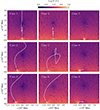 |
Fig. 1. Magnetic configuration at the initial times for the cases. In colour, we plot the magnitude of the magnetic field. The projections of the magnetic field lines into the xy-plane are represented with black lines, and the trajectories of the MFR with white lines. |
Also, considering the results obtained by Sahade et al. (2022), we calculated the magnetic flux of the MFR and its strapping field. Those closed field lines of the HS that overlie the MFR constitute the strapping field (blue lines displayed in case 5 in Fig. 2). These lines form a MC that constrain the MFR (represented by a closed light green line in Fig. 2) eruption. Given the symmetry axis, we calculated the poloidal magnetic flux per unit length, for both the MFR and the MC, using
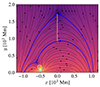 |
Fig. 2. Magnetic flux calculation. The black lines represent the projection of the magnetic field lines into the xy-plane magnetic field lines. The blue lines delineate the MC, and the light green ring symbolises the MFR. To ascertain the magnetic flux, integration is performed along the vertical yellow lines. |
For simplicity, we defined γ over a line of x = c, where c is a constant. Consequently, B⊥ = Bx and ds = dy. For the calculation of the MFR flux (ϕBp, MFR), c is determined by the x−position of its centre and y limits of γ are defined by the height of the MFR centre and the last closed field line belonging to the MFR (vertical yellow line centred in the MFR shown in Fig. 2). To calculate the MC flux, ϕBp, MC, we chose c and y limits of γ are defined by the height of the first and last closed magnetic field lines, tied to the chromosphere, located above the MFR (in Fig. 2, the vertical yellow line located at x = 0).
3. Results
3.1. Topology and dynamic behaviour
Below we group the cases according to their reconnection dynamics. We define successful ascent cases as those in which the MFR rises beyond the top of the HS and maintains an upward trajectory until the end of the simulation. The unsuccessful ascent cases can be further split into failed ascents where the ascent starts but then stalls and confined ascents where the ascent does not begin to start with.
3.1.1. Cases 1 and 4
In these cases, the MFR is centred inside the HS (xMFR = 0) and the MFR polarity is inverted compared to the HS polarity. The combination of MFR and HS magnetic fields creates a secondary null point above the MFR (see Fig. 1). However, the background HS field strength differs by a factor of two (Table 1) between the cases.
Case 1 with the weaker HS field is a successful ascent (see the evolution in the animated version). Figure 3 displays the evolution of the current jz and the z component of the magnetic field. Initially, as the MFR rises, the null point collapses into a current sheet that becomes stretched around the flux rope (see the second column). The change in connectivity as a result of reconnection within this current layer is shown schematically in Fig. 4. Reconnection in this current sheet acts to reduce the overlying strapping field: the outer magnetic field of the MFR (the blue line in the left panel) reconnects with the overlying magnetic field of the MC (black line), which is converted into a new magnetic field line below the MFR (the new green line in the right panel). In effect, the reconnection ahead of the MFR allows it to ‘tunnel’ through the strapping field at the expense of loosing outer layers of poloidal magnetic flux in the process.
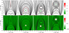 |
Fig. 3. Upper panel: Evolution of the current jz (in units of 10−10 G cm−1) for case 1. Bottom panel: Evolution of Bz (in units of G) within the MFR. The initial time is depicted in the first panel, t = 5000 s in second panel, t = 16 000 s in third panel, and t = 17 000 s in the last panel. The black lines represent the projection of the magnetic field lines into the xy-plane. An associated movie is available online. |
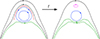 |
Fig. 4. Diagram illustrating the magnetic reconnection occurring in cases 1 and 4. Black lines represent the magnetic field lines of the MC, blue lines the magnetic field lines of the MFR, green lines the arcade below the MFR, and the pink line the magnetic island formed. The red line highlights the current sheet region between the MFR and the MC. |
This reconnection is similar to that of the magnetic breakout model (Antiochos et al. 1999) for CME eruptions. However, the reconnection in our model differs from classic breakout reconnection in some key ways. Firstly, in the breakout model, the initial null point is a feature of a quadra-polar surface magnetic flux distribution, whereas here we have a background flux distribution that is bipolar. Secondly, in the breakout model the presence of the four flux regions in the background magnetic field means that strapping field is reconnected into two adjacent ‘lobe’ flux systems. This facilitates the eruption purely by reducing the overall downward magnetic tension on the flux rope channel. Here the strapping field is moved behind the flux rope, reducing the magnetic tension in the same manner but also adding additional magnetic pressure and tension behind the flux rope, which further drives it upwards. However, in the breakout model, a flare current layer also forms behind the flux rope, which our model lacks. Reconnection in the flare current layer increases the magnetic flux of the flux rope, aiding in the eruption. Nevertheless, despite the differences, there are still clear similarities between the evolution we see in our simulation and previous breakout simulations, which will be discussed further below. We also note that Titov et al. (2022) identified similar breakout-like reconnection in a bipolar magnetic configuration, referring to it as ‘breakthrough’ reconnection. However, their configuration also contained a flare current layer so is again not quite the same as the reconnection dynamics in these simulations. For simplicity we refer to the reconnection in our simulations as ‘null point’ reconnection, but will highlight the similarities to previous breakout simulations where appropriate.
Returning to the evolution in case 1, not long after the onset of reconnection in the current sheet ahead of the MFR, a magnetic island forms and quickly grows to become comparable in size to the MFR itself (Fig. 3 central panels). The field configuration is also shown schematically in Fig. 4. The large size that the island grows to is an artefact of the symmetry of our system (see e.g. MacNeice et al. 2004). The formation of the island inhibits the initial rise of the flux rope, which then experiences a bounce-back before eventually ascending (Fig. 3, right panels).
Case 4 has a similar initial evolution, but with much less initial expansion of the MFR due to the stronger HS field. In this case the ascent fails when the stronger strapping field absorbs the initial rise of the MFR, which sets up an oscillation of the MFR beneath the apex of the HS (see the trajectory in Fig. 1). Also, the null point reconnection erodes not just the outer flux surfaces of the MFR, but continues all the way to its core. Eventually, the MFR is destroyed entirely (see evolution of jz in upper panels of Fig. A.1, and in the animated version). A by-product of this is that the axial flux of the flux rope becomes spread out along closed loops within the HS (bottom panels of Fig. A.1). Again, there are parallels with previous work on jets and confined eruptions invoking breakout reconnection where in those cases the breakout reconnection proceeds until it reaches the core of the erupting flux rope channel, transferring its twist to adjacent flux systems (e.g. DeVore & Antiochos 2008; Doyle et al. 2019).
3.1.2. Cases 2, 3, 5, and 6
In all these cases the MFR’s initial position is shifted to the left. Again the MFR has a magnetic polarity that is opposite to that of the HS but now the null point is initially present above and to the left of the MFR (Fig. 1). The MFR in cases 3 and 6 is placed further to the left than in cases 2 and 5, and within each pairing two HS field strengths are considered (see Table 1 for details).
In all cases the MFR initially rises towards the null point, deflecting the eruption towards the left flank of the HS before being redirected back towards the apex of the HS (see the trajectories in Fig. 1). As in the previous cases, the expansion of the MFR collapses the null point into a current sheet, inducing reconnection. The flux transfer induced by this reconnection is shown schematically in Fig. 5. Due to the asymmetry of the system, when islands form in the current layer they are quickly ejected so do not grow to sizes large enough to affect the overall ascent. Cases 2, 3, and 6 are successful ascent and follow a similar evolution (see the animated versions). Figure A.2 shows the evolution of case 6 as an example (see also the animated version). The induced reconnection tunnels the MFR towards the open flux, discussed further in Sect. 3.2, reducing the overall strapping flux and ultimately allowing the MFR to continue on its upward trajectory when it reaches the apex of the HS (Fig. A.2, right panels).
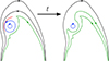 |
Fig. 5. Diagram illustrating later magnetic reconnection occurring in cases 2, 3, 5, and 6. Black lines represent the magnetic field lines of the MC, blue lines the magnetic field lines of the MFR, and green lines the arcade below the MFR. The red line highlights the current sheet region between the MFR and the MC. |
By contrast, the ascent in case 5 fails. In this case, as in case 4, the stronger overlying field absorbs the initial rise of the MFR, redirecting it downwards where it then bounces back and forth within the HS. Eventually, the null point reconnection reaches the core of the MFR, spreading its axial field component along the HS field (see Fig. A.3 and its animated version).
3.1.3. Cases 7, 8, and 9
In these cases, the MFR has the same polarity as the HS magnetic field. In case 7, where the MFR is positioned directly below the apex of the HS, the symmetry of the system leads to two null points, one on each side of the MFR on the lower boundary. In cases 8 and 9 where the MFR is displaced to the left, a single null point initially resides below and to the right of it (Fig. 1). No ascent occurs in these cases, and the MFRs remain confined to near their initial position (see the animated versions). The evolution in case 9 is shown in Fig. A.4 as an example. The MFR first expands and moves to the right, before relaxing to a new equilibrium.
3.2. Analysis of magnetic fluxes versus ascent behaviour
In this section we analyse the losses and ratios of the magnetic fluxes per unit length of the MFR and the MC. This analysis will help quantify the ascent behaviour of the different systems.
In Table 1 we also show the poloidal (in-plane) magnetic fluxes per unit length (ϕBp) calculated for the MC and MFR at t = 0 (calculated as described in Sect. 2.3; see also Fig. 2). The change in time (ϕBp(t)−ϕBp(0)) throughout each simulation of both quantities is shown in Fig. 6. It can be seen that both the MC and MFR lose poloidal magnetic flux per unit length over time, with the losses being lower in the MC compared to the MFR. This is due to the competing effects of the reconnection occurring in the system. For cases where the null point is above the MFR initially, the null point reconnection induced by the motion of the MFR reduces the flux of the MFR and MC equally. The reconnected MC flux is transferred behind the MFR as it tunnels upwards. However, at the same time reconnection in the HS current sheet adds some flux to the MC. For cases 1–6, we show a significant decrease in the flux of the MC, indicating that despite this contribution, the null point reconnection plays a predominant role in reducing the flux in the MC. For cases where the null point is below the flux rope axis, the reconnection tunnels the flux rope laterally, and deeper into the closed field, adding flux to the MC from the MFR in addition to the flux added by the HS current sheet reconnection.
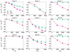 |
Fig. 6. Evolution of the magnetic flux per unit length difference relative to its initial value for both the MC (green lines) and the MFR (pink lines). |
To analyse the evolution of magnetic flux per unit length in both the MC and MFR over time, Fig. 7 shows the absolute values of the ratios of the poloidal magnetic fluxes per unit length between a time ‘t’ with respect to an initial time ‘0’ for the MC ( ) and for the MFR (
 ). From here, we observe that the trend of flux decay continues over time, both for the MC (
 ) and the MFR (
 ) in all cases. However, we note that for successful and unsuccessful ascent cases, these decays differ. Unsuccessful ascent cases (cases 4, 5, 7, 8, and 9) show that the decay of the MC flux is smaller than that of the MFR. The opposite is observed for successful ascent cases.
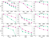 |
Fig. 7. Evolution of magnetic flux per unit length decay rate for the MC (green lines) and MFR (pink lines) over time. |
The key difference between the successful and unsuccessful ascent (failed and confined) cases that helps explain this is the initial poloidal flux within the MFR (see Table 1). In the successful ascent cases the poloidal flux of the flux rope is a relatively high fraction of the MC flux, leading to a larger relative drop in MC flux than MFR flux as it tunnels outwards.
This can be seen more clearly when the fluxes of the MFR and MC are compared with time. Figure 8 shows the ratio between the magnetic flux per unit length of the MFR and the MC (qMFR/MC = ϕBp, MFR(t)/ϕBp, MC(t)) over time. Once again, there are distinct differences in behaviour between unsuccessful and successful ascent cases. In unsuccessful ascent cases, the ratios decrease with time indicating a relative increase in the strapping flux of the MC, while the successful ascent cases exhibit an ascending trend. This is indicative of a relative drop in the strapping flux of the MC relative to the flux of the flux rope. This is also a typical feature of breakout-type eruptions (e.g. Antiochos et al. 1999) and indicates that in a similar manner the null point reconnection in our simulations is playing a key role in facilitating these successful ascent through the reduction of the overlying flux. The transition from unsuccessful to successful ascent occurs around qMFR/MC ∼ 1.5. With the successful ascent cases having qMFR/MC ≳ 1.5 throughout their evolution.
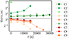 |
Fig. 8. Evolution of the ratio between the MFR and MC magnetic flux per unit length over time. Green represents successful ascent cases and red unsuccessful cases. The dashed black line marks the threshold of 1.5. |
4. Conclusions
We have considered the influence of the HS topology on the ascent behaviour and deflection of MFR eruptions. The limited parameter study performed was broad enough to include both stable and unstable cases and with differing levels of asymmetry in the flux rope location.
To analyse the ascent behaviour, as mentioned in Sect. 2.1, we selected a non-equilibrium configuration for the MFR immersed in an HS background. This setup results in an early deceleration of the MFR, with the interaction of the flux rope with its surroundings being the focus of our study. Although this model cannot fully reproduce the initial onset of the ejection (the slow-to-fast rise phase), we define a successful ascent as the MFR reaching beyond 2.5 R⊙, which remains a reasonable and consistent threshold within the framework of our analysis.
Regarding the flux rope deflection, our findings confirm previous results, showing that the MFR is deflected towards regions with weaker magnetic fields, guided by the topology of the magnetic field lines (e.g. Wang et al. 2023; Ben-Nun et al. 2023; Sahade et al. 2023). In the HS topology, this region corresponds to the heliospheric current sheet. In cases where a null point was initially present above the flux rope, the null point also served as a low magnetic field region that the flux rope deflected towards. As shown in, for example, case 3, the combination of the two features can lead to a change in the deflection direction that results in a curved path for the flux rope during the eruption. A comparable behaviour was noted in Yang et al. (2018). A filament positioned adjacent to a heliospheric streamer initially underwent a northward eruption and subsequently deflected southwards towards the magnetic minimum in the streamer configuration. However, we note that our simulations are 2.5D and this pre-supposes that 3D effects such as twist transfer along field lines, which can also lead to deflections, do not occur (Wyper et al. 2021).
Null point reconnection can play either a stabilising or destabilising role in the ascent depending on the configuration. Reconnection occurred in our simulations when the null point was initially above the inserted flux rope, which then rapidly collapsed into a current layer once the simulation was underway. The reconnection in this layer acts to erode the outer poloidal flux of the flux rope while also reducing the strapping flux of the MC. When the strapping flux of the MC is sufficiently great, the initial ascent of the MFR stalls and the MFR then oscillates in position while the reconnection erodes the flux of the flux rope until it is destroyed (cases 4 and 5).
However, in other instances (cases 1, 2, 3, and 6) the reconnection acted to enable the ascent. In such cases the poloidal flux of the flux rope was initially large enough that the erosion of poloidal flux did not reach the core of the flux rope, destroying it as in the cases with failed ascents. Instead, the flux rope core maintained its coherence as the null point reconnection tunnelled it through the strapping flux. In the asymmetric cases (2, 3, and 6) this brought it closer to the open-closed boundary and ultimately into the open field in a manner similar to that shown by Masson et al. (2013) for a breakout-type eruption. When the configuration was symmetric, the reconnection simply reduced the overlying flux enough that the flux rope became unstable (case 1). Finally, in the absence of reconnection, when the null point is initially beneath or adjacent to the inserted flux rope (cases 7, 8, and 9) we find that the flux rope motion is rapidly stabilised.
At this point, it is appropriate to mention that the symmetry of the system in certain simulations, such as case 1, can lead to the generation of an artificially large island ahead of the flux rope. These islands likely hinder the ascent by suppressing the null point or breakout reconnection. However, the fact that the flux rope still rises despite this suppression suggests that it is particularly unstable. We also note that such large islands have been seen in previous studies (e.g. MacNeice et al. 2004).
As noted in previous work (e.g. Amari et al. 2018; Sahade et al. 2022), we also find that the magnetic flux of the MC plays a crucial role in the ascent process. This occurs both through the bodily confinement of the flux rope and by dictating the extent of the reconnection dynamics. Analysing magnetic fluxes within the system and their evolution in time, we find a strong correlation between the ascent occurrence and the ratio of the magnetic fluxes in the MFR and MC. Although it does not directly predict the eruptive nature of the MFR, this ratio provides valuable insights into its evolution and the conditions influencing its behaviour. We have identified a critical value of this ratio that serves as a distinguishing factor for ascent outcomes. Specifically, when the poloidal flux of the MFR is greater than 1.5 times the strapping flux of the MC (qMFR/MC > 1.5), an ascent is triggered. However, we note that our simulations lacked a solar wind, which would be expected to open high-lying magnetic field lines and thus aid the ascent. Therefore, the qMFR/MC threshold we have identified for HSs is likely an upper bound.
Another consequence of the absence of solar wind emulation is the unbalanced reconnection in the heliospheric current sheet. As mentioned in Sect. 3.2, magnetic field lines reconnect at the apex of the HS, contributing to the flux of the strapping field. Were a solar wind included, this addition of magnetic flux would be balanced on average by the re-opening of a closed field pulled out by the solar wind (e.g. Higginson et al. 2017). Nonetheless, our results indicate that the flux contribution from this reconnection to the MC is negligible over the time frame of the eruptions we investigated. In all cases, the null point reconnection plays a dominant role, and the strapping flux consistently decreases.
It is important to note that the threshold for flux ratios depends implicitly on the position of the null point. The time evolution captures this dynamic, as the cases with the null point below or adjacent to the MFR have a ratio that decreases over time. We can conclude that while knowledge of the null point’s position is crucial, it is not sufficient. The flux ratio must also exceed the threshold. For future work, configurations should be considered in which the null point is below an MFR that is unstable to ascent to see if the flux ratio remains robust in those cases. However, this falls outside the current scope of our study, which focuses on cases dominated by reconnection above or adjacent to the flux rope.
In the future it would be interesting to consider how this threshold could be extended to three dimensions, or how it relates to other thresholds for ascent behaviour based on the magnetic configurations that have been identified in other studies (e.g. Rice & Yeates 2022). Regardless of the specifics, what is clear is that to understand flux rope ascents and be able to reliably predict whether an eruption will be successful, it is crucial to account for not only the properties of the flux rope, but also how it interacts with its magnetic surroundings.
Data availability
Movies associated to Figs. 3, A1–A.4 are available at https://www.aanda.org
Acknowledgments
MC and GK are members of the Carrera del Investigador Científico (CONICET). MC knowledges support from the DynaSun project, which has received funding under the Horizon Europe programme of the European Union, grant agreement no. 101131534. Views and opinions expressed are however those of the author only and do not necessarily reflect those of the European Union and therefore the European Union cannot be held responsible for them. PFW was supported by STFC (UK) consortium grant ST/W00108X/1 and a Leverhulme Trust project grant. AS was supported by an appointment to the NASA Postdoctoral Program at the NASA Goddard Space Flight Center, administered by Oak Ridge Associated Universities under contract with NASA. MC, GK and AS acknowledge support from CONICET under grant PIP number 11220200103150CO. OEKR was supported by a UKRI/STFC PhD studentship. We thank Anthony Yeates and Silvina Guidoni for useful discussions. MC also acknowledges the hospitality of the Department of Mathematical Sciences were part of this work was carried out. Also, we thank the Centro de Cómputo de Alto Desempeño (UNC), where the simulations were performed. The software used in this work was developed in part by the DOE NNSA- and DOE Office of Science-supported Flash Center for Computational Science at the University of Chicago and the University of Rochester.
References
- Amari, T., Canou, A., Aly, J.-J., Delyon, F., & Alauzet, F. 2018, Nature, 554, 211 [NASA ADS] [CrossRef] [Google Scholar]
- Antiochos, S. K., DeVore, C. R., & Klimchuk, J. A. 1999, ApJ, 510, 485 [Google Scholar]
- Ben-Nun, M., Török, T., Palmerio, E., et al. 2023, ApJ, 957, 74 [Google Scholar]
- DeVore, C. R., & Antiochos, S. K. 2008, ApJ, 680, 740 [NASA ADS] [CrossRef] [Google Scholar]
- Doyle, L., Wyper, P. F., Scullion, E., et al. 2019, ApJ, 887, 246 [Google Scholar]
- Forbes, T. G. 1990, J. Geophys. Res., 95, 11919 [NASA ADS] [CrossRef] [Google Scholar]
- Forbes, T. G. 2000, J. Geophys. Res., 105, 23153 [Google Scholar]
- Fryxell, B., Olson, K., Ricker, P., et al. 2000, ApJS, 131, 273 [Google Scholar]
- Higginson, A. K., Antiochos, S. K., DeVore, C. R., Wyper, P. F., & Zurbuchen, T. H. 2017, ApJ, 837, 113 [Google Scholar]
- Hu, Y. Q. 2001, Sol. Phys., 200, 115 [Google Scholar]
- Karpen, J., Kumar, P., Wyper, P., DeVore, C. R., & Antiochos, S. 2024, ApJ, 966, 27 [Google Scholar]
- Krause, G. 2019, A&A, 631, A68 [NASA ADS] [CrossRef] [EDP Sciences] [Google Scholar]
- Krause, G., Cécere, M., Zurbriggen, E., et al. 2018, MNRAS, 474, 770 [Google Scholar]
- Lee, D., & Deane, A. E. 2009, J. Comput. Phys., 228, 952 [NASA ADS] [CrossRef] [Google Scholar]
- MacNeice, P., Antiochos, S. K., Phillips, A., et al. 2004, ApJ, 614, 1028 [NASA ADS] [CrossRef] [Google Scholar]
- Masson, S., Antiochos, S. K., & DeVore, C. R. 2013, ApJ, 771, 82 [NASA ADS] [CrossRef] [Google Scholar]
- Mei, Z., Shen, C., Wu, N., et al. 2012, MNRAS, 425, 2824 [NASA ADS] [CrossRef] [Google Scholar]
- Pariat, E., Leake, J. E., Valori, G., et al. 2017, A&A, 601, A125 [CrossRef] [EDP Sciences] [Google Scholar]
- Rice, O. E. K., & Yeates, A. R. 2022, Front. Astron. Space Sci., 9, 849135 [NASA ADS] [CrossRef] [Google Scholar]
- Rice, O. E. K., & Yeates, A. R. 2023, ApJ, 955, 114 [Google Scholar]
- Sahade, A., Cécere, M., Sieyra, M. V., et al. 2022, A&A, 662, A113 [NASA ADS] [CrossRef] [EDP Sciences] [Google Scholar]
- Sahade, A., Vourlidas, A., Balmaceda, L. A., & Cécere, M. 2023, ApJ, 953, 150 [Google Scholar]
- Talpeanu, D. C., Poedts, S., D’Huys, E., Mierla, M., & Richardson, I. G. 2022, A&A, 663, A32 [NASA ADS] [CrossRef] [EDP Sciences] [Google Scholar]
- Titov, V. S., Downs, C., Török, T., & Linker, J. A. 2022, ApJ, 936, 121 [Google Scholar]
- Wang, J., Liu, S., & Luo, B. 2023, Adv. Space Res., 72, 5263 [Google Scholar]
- Wyper, P. F., Antiochos, S. K., DeVore, C. R., et al. 2021, ApJ, 909, 54 [NASA ADS] [CrossRef] [Google Scholar]
- Yang, J., Dai, J., Chen, H., Li, H., & Jiang, Y. 2018, ApJ, 862, 86 [CrossRef] [Google Scholar]
- Zhang, Q., Wang, Y., Liu, R., et al. 2020, ApJ, 898, L12 [Google Scholar]
- Zhuang, B., Hu, Y., Wang, Y., et al. 2018, J. Geophys. Res. (Space Phys.), 123, 2513 [Google Scholar]
Appendix A: Figures of the evolution of selected cases
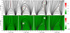 |
Fig. A.2. Similar to Fig. 3 but for case 6. The initial time is displayed in the first panel, t = 5000 s in second panel, t = 10000 s in third panel, and t = 15000 s in the last panel. An associated movie is available online. |
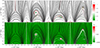 |
Fig. A.3. Similar to Fig. 3 but for case 5. The initial time is displayed in the first panel, t = 5000 s in second panel, t = 15000 s in third panel, and t = 24000 s in the last panel. An associated movie is available online. |
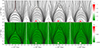 |
Fig. A.4. Similar to Fig. 3 but for case 9. The initial time is displayed in the first panel, t = 5000 s in second panel, t = 10000 s in third panel, and t = 25000 s in the last panel. An associated movie is available online. |
All Tables
All Figures
|
Fig. 1. Magnetic configuration at the initial times for the cases. In colour, we plot the magnitude of the magnetic field. The projections of the magnetic field lines into the xy-plane are represented with black lines, and the trajectories of the MFR with white lines. |
| In the text | |
|
Fig. 2. Magnetic flux calculation. The black lines represent the projection of the magnetic field lines into the xy-plane magnetic field lines. The blue lines delineate the MC, and the light green ring symbolises the MFR. To ascertain the magnetic flux, integration is performed along the vertical yellow lines. |
| In the text | |
|
Fig. 3. Upper panel: Evolution of the current jz (in units of 10−10 G cm−1) for case 1. Bottom panel: Evolution of Bz (in units of G) within the MFR. The initial time is depicted in the first panel, t = 5000 s in second panel, t = 16 000 s in third panel, and t = 17 000 s in the last panel. The black lines represent the projection of the magnetic field lines into the xy-plane. An associated movie is available online. |
| In the text | |
|
Fig. 4. Diagram illustrating the magnetic reconnection occurring in cases 1 and 4. Black lines represent the magnetic field lines of the MC, blue lines the magnetic field lines of the MFR, green lines the arcade below the MFR, and the pink line the magnetic island formed. The red line highlights the current sheet region between the MFR and the MC. |
| In the text | |
|
Fig. 5. Diagram illustrating later magnetic reconnection occurring in cases 2, 3, 5, and 6. Black lines represent the magnetic field lines of the MC, blue lines the magnetic field lines of the MFR, and green lines the arcade below the MFR. The red line highlights the current sheet region between the MFR and the MC. |
| In the text | |
|
Fig. 6. Evolution of the magnetic flux per unit length difference relative to its initial value for both the MC (green lines) and the MFR (pink lines). |
| In the text | |
|
Fig. 7. Evolution of magnetic flux per unit length decay rate for the MC (green lines) and MFR (pink lines) over time. |
| In the text | |
|
Fig. 8. Evolution of the ratio between the MFR and MC magnetic flux per unit length over time. Green represents successful ascent cases and red unsuccessful cases. The dashed black line marks the threshold of 1.5. |
| In the text | |
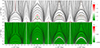 |
Fig. A.1. Same as Fig. 3 but for case 4. An associated movie is available online. |
| In the text | |
|
Fig. A.2. Similar to Fig. 3 but for case 6. The initial time is displayed in the first panel, t = 5000 s in second panel, t = 10000 s in third panel, and t = 15000 s in the last panel. An associated movie is available online. |
| In the text | |
|
Fig. A.3. Similar to Fig. 3 but for case 5. The initial time is displayed in the first panel, t = 5000 s in second panel, t = 15000 s in third panel, and t = 24000 s in the last panel. An associated movie is available online. |
| In the text | |
|
Fig. A.4. Similar to Fig. 3 but for case 9. The initial time is displayed in the first panel, t = 5000 s in second panel, t = 10000 s in third panel, and t = 25000 s in the last panel. An associated movie is available online. |
| In the text | |
Current usage metrics show cumulative count of Article Views (full-text article views including HTML views, PDF and ePub downloads, according to the available data) and Abstracts Views on Vision4Press platform.
Data correspond to usage on the plateform after 2015. The current usage metrics is available 48-96 hours after online publication and is updated daily on week days.
Initial download of the metrics may take a while.