| Issue |
A&A
Volume 709, May 2026
|
|
|---|---|---|
| Article Number | A96 | |
| Number of page(s) | 10 | |
| Section | Interstellar and circumstellar matter | |
| DOI | https://doi.org/10.1051/0004-6361/202557676 | |
| Published online | 05 May 2026 | |
Search for long-term variability of HESS J1745-290
1
University of Southern Denmark,
Denmark
2
Astronomy & Astrophysics Section, School of Cosmic Physics, Dublin Institute for Advanced Studies, DIAS Dunsink Observatory,
Dublin
D15 XR2R,
Ireland
3
Max-Planck-Institut für Kernphysik,
PO Box 103980,
69029
Heidelberg,
Germany
4
University of Namibia, Department of Physics,
Private Bag 13301,
Windhoek
10005,
Namibia
5
Centre for Space Research, North-West University,
Potchefstroom
2520,
South Africa
6
Institut für Physik und Astronomie, Universität Potsdam,
Karl-Liebknecht-Strasse 24/25,
14476
Potsdam,
Germany
7
Deutsches Elektronen-Synchrotron DESY,
Platanenallee 6,
15738
Zeuthen,
Germany
8
Institut für Physik, Humboldt-Universität zu Berlin,
Newtonstr. 15,
12489
Berlin,
Germany
9
LUX, Observatoire de Paris, Université PSL, CNRS, Sorbonne Université,
5 Pl. Jules Janssen,
92190
Meudon,
France
10
Sorbonne Université, CNRS/IN2P3, Laboratoire de Physique Nucléaire, et de Hautes Energies, LPNHE,
4 place Jussieu,
75005
Paris,
France
11
IRFU, CEA, Université Paris-Saclay,
91191
Gif-sur-Yvette,
France
12
Friedrich-Alexander-Universität Erlangen-Nürnberg, Erlangen Centre for Astroparticle Physics,
Nikolaus-Fiebiger-Str. 2,
91058
Erlangen,
Germany
13
Université Paris Cité, CNRS, Astroparticule et Cosmologie,
75013
Paris,
France
14
School of Physics, University of the Witwatersrand,
1 Jan Smuts Avenue, Braamfontein,
Johannesburg
2050,
South Africa
15
School of Physical Sciences and Centre for Astrophysics & Relativity, Dublin City University,
Glasnevin,
Dublin
D09 W6Y4,
Ireland
16
University of Oxford, Department of Physics,
Denys Wilkinson Building, Keble Road,
Oxford
OX1 3RH,
UK
17
Laboratoire Leprince-Ringuet, École Polytechnique, CNRS, Institut Polytechnique de Paris,
91128
Palaiseau,
France
18
Aix Marseille Université, CNRS/IN2P3, CPPM,
Marseille,
France
19
Laboratoire Univers et Particules de Montpellier, Université Montpellier,
CNRS/IN2P3, CC 72, Place Eugène Bataillon,
34095
Montpellier Cedex 5,
France
20
Université Bordeaux, CNRS, LP2I Bordeaux, UMR 5797,
33170
Gradignan,
France
21
School of Science, Western Sydney University,
Locked Bag 1797,
Penrith South DC,
NSW 2751,
Australia
22
Landessternwarte, Universität Heidelberg,
Königstuhl,
69117
Heidelberg,
Germany
23
Institut für Astronomie und Astrophysik, Universität Tübingen,
Sand 1,
72076
Tübingen,
Germany
24
Universität Innsbruck, Institut für Astro- und Teilchenphysik,
Technikerstraße 25,
6020
Innsbruck,
Austria
25
Universität Hamburg, Institut für Experimentalphysik,
Luruper Chaussee 149,
22761
Hamburg,
Germany
26
Obserwatorium Astronomiczne, Uniwersytet Jagielloński,
ul. Orla 171,
30-244
Kraków,
Poland
27
Nicolaus Copernicus Astronomical Center, Polish Academy of Sciences,
ul. Bartycka 18,
00-716
Warsaw,
Poland
28
Instytut Fizyki Jacadrowej PAN,
ul. Radzikowskiego 152, ul. Radzikowskiego 152,
31-342
Kraków,
Poland
29
GRAPPA, Anton Pannekoek Institute for Astronomy, University of Amsterdam,
Science Park 904,
1098 XH
Amsterdam,
The Netherlands
30
School of Physical Sciences, University of Adelaide,
Adelaide
5005,
Australia
31
Yerevan Physics Institute,
2 Alikhanian Brothers St.,
0036
Yerevan,
Armenia
32
Department of Physics, Konan University,
8-9-1 Okamoto, Higashinada, Kobe,
Hyogo
658-8501,
Japan
33
Kapteyn Astronomical Institute, University of Groningen,
Landleven 12,
9747 AD
Groningen,
The Netherlands
★ Corresponding author: This email address is being protected from spambots. You need JavaScript enabled to view it.
Received:
13
October
2025
Accepted:
14
February
2026
Abstract
At the center of our Galaxy lies the bright γ-ray point-like source HESS J1745-290, which is compatible in position with Sgr A⋆, although an association between the two remains uncertain. Using data obtained between 2004 and 2019 with the High Energy Stereoscopic System (H.E.S.S.) on the Galactic center region, we studied the variability of HESS J1745-290 over 353 hours of observations collected over 16 years, representing the largest dataset gathered yet on this region at TeV energies. We performed a 3D maximum-likelihood analysis of the central source and the diffuse γ-ray emission in the Galactic center region. This analysis allowed us to extract the spectral and morphological intrinsic behavior of the two components. By performing this analysis on an annual basis, we derived the light curve of HESS J1745-290 and the diffuse emission over the past 16 years. The 3D maximum-likelihood analysis method allowed us to separate the central source from the overlapping diffuse emission, enabling a recalibration of the former by the latter and alleviating some of the systematic effects. We find no long-term or yearly variability. We also provide an estimate of the sensitivity of H.E.S.S. to variation of this specific source over 16 years. We rule out any yearly γ-ray flux variation of this source larger than 30%, as well as any linear flux variation exceeding 30% over this time period.
Key words: Galaxy: center / gamma rays: general / gamma rays: ISM
© The Authors 2026
 Open Access article, published by EDP Sciences, under the terms of the Creative Commons Attribution License (https://creativecommons.org/licenses/by/4.0), which permits unrestricted use, distribution, and reproduction in any medium, provided the original work is properly cited.
This article is published in open access under the Subscribe to Open model. This email address is being protected from spambots. You need JavaScript enabled to view it. to support open access publication.
1 Introduction
The Galactic center (GC) is a prime observation region for very high energy (VHE) γ rays. Various observatories, including the High Energy Stereoscopic System (H.E.S.S.) (Aharonian et al. 2004, 2006a, 2008, 2009; Acero et al. 2010), the Major Atmospheric Gamma-ray Imaging Cherenkov Telescope (MAGIC) (Albert et al. 2006; MAGIC Collaboration 2020), and the Very Energetic Radiation Imaging Telescope Array System (VERI-TAS) (Archer et al. 2014, 2016; Adams et al. 2021) have detected the point-like source HESS J1745-290. This source is centered at the Galactic coordinates l = 359.944◦, b = −0.046◦, with a 13 arcsec uncertainty and an upper bound on its extension of about 1.2 arcmin (Acero et al. 2010).
Although HESS J1745-290 is the most prominent feature of the region, H.E.S.S. has also identified diffuse emission extending over 200 pc along the inner Galactic plane(Aharonian et al. 2006b; H.E.S.S. Collaboration 2018). This diffuse emission most likely indicates a high density of cosmic rays in the central region of the Galaxy (H.E.S.S. Collaboration 2016), which interact with the central molecular zone (CMZ) to produce γ rays via proton-proton interaction and neutral pion decay.
Despite numerous studies, the physical origin of HESS J1745-290 remains an open question. Potential sources such as the supernova remnant Sgr A East have been ruled out based on their extension and positional incompatibility with the source (Acero et al. 2010). The pulsar wind nebula (PWN) candidate G359.95-0.04 remains a plausible counterpart, as it is compatible in both position and energetics with the source (Wang et al. 2006; Hinton & Aharonian 2007). However, the estimated magnetic field in the vicinity of GC might be too large for this scenario to be plausible (Kistler 2015). The super-massive black hole (SMBH) at the center of our Galaxy, Sgr A⋆, is therefore a plausible origin of the γ-ray source, as it is fully compatible in position and its accretion flow provides a site of particle acceleration.
Across the electromagnetic spectrum, Sgr A⋆ shows high and rapid variability, with the highest flux variations observed in the X-ray and infrared (IR) domain (see overviews Genzel et al. 2010; Witzel et al. 2021). X-ray observatories have observed regular flares that last a few hours and occur daily. These events have varying intensities that can reach up to two orders of magnitude above the quiescent level (for Chandra, see Baganoff et al. 2001; Neilsen et al. 2015; for Swift, see Andrés et al. 2022). In the IR domain, the emission of Sgr A⋆ shows high variability (Genzel et al. 2003); however, additional individual flaring events have recently been identified in the NIR range, with amplitudes reaching a factor of two on timescales of ∼20 minutes (Do et al. 2019; GRAVITY Collaboration 2020).
The link between IR and X-ray flares is not completely straightforward, as X-ray flares are usually accompanied by a flare-type event in IR (Eckart et al. 2004), but the reverse is not always true. The emission mechanism behind these flares is generally interpreted as lepton-based synchrotron and/or Compton-scattering emission occurring in the inner accretion flow, relatively close to the SMBH (from a few Schwarzschild radii, RS , up to ∼102 RS ) (Yuan et al. 2003; Dodds-Eden et al. 2010; Ponti et al. 2017; GRAVITY Collaboration 2021).
The high-energy particles that produce the γ-ray signal can be accelerated close to the SMBH, but they can also escape the accretion flow and interact farther in the surrounding medium, depending on the particle transport conditions and the matter distribution. For instance, Liu et al. (2006) proposed that protons are accelerated by stochastic processes within the inner 20 RS and escape and scatter in the inner few parsecs to produce the TeV emission. As noted by Ballantyne et al. (2007) and Linden et al. (2012) , the most plausible target for producing γ rays is the circumnuclear disk (CND) (Christopher et al. 2005), a 1.5 pc radius ring-like structure of dense molecular matter surrounding Sgr A⋆. Depending on the assumed particle transport hypotheses, the GC VHE source could therefore reflect the history of particle acceleration in the vicinity of the SMBH over shorter or longer timescales and remain stable on timescales of years or more (Ballantyne et al. 2011; Chernyakova et al. 2011; Guo et al. 2013). The long-term variability of HESS J1745-290 is therefore a key observable to determine its nature and possibly constrain the particle acceleration processes in Sgr A⋆. Whipple first studied the variability of the GC at VHE between 2000 and 2004 (Kosack et al. 2004) and showed that the source’s flux was consistent with being constant. Another study in 2009 (Aharonian et al. 2009) used the first three years of H.E.S.S. data (2004–2006) to search for variability on 28-minute timescales, hour-long flares, and quasi-periodic oscillations (QPOs), but detected no significant signals. More recent studies by MAGIC (Ahnen et al. 2017) and VERITAS (Archer et al. 2014; Adams et al. 2021), corroborate this apparent stability over daily to monthly timescales. In addition, attempts to detect counterparts of X-ray flares with H.E.S.S. have so far been unsuccessful (see Aharonian et al. (2008) for the joint H.E.S.S.-Chandra observation campaign in 2006).
In this work, we investigate the potential variability of HESS J1745-290 over timescales of years. We take advantage of the large H.E.S.S. observation database to measure the yearly evolution of the VHE flux over the 16-year period from 2004 to 2019, driven by the parsec-scale γ-ray emission implied by models.
After describing how we selected and processed the 16 years of H.E.S.S. data on the GC (Section 2), we present our methodology in two parts. First, we describe the spectro-morphological analysis of HESS J1745-290 and its surroundings (Section 3), then the study of time variability of HESS J1745-290 (Section 4). In Section 5, we reassess the sensitivity of the H.E.S.S. survey to several theoretical time variation models. Finally, in Section 6, we discuss the significance of these results in the context of existing knowledge of Sgr A⋆ variability across the electromagnetic spectrum.
2 Data reduction
The H.E.S.S. array consists of five imaging atmospheric cherenkov telescopes (IACTs), located in Namibia, and has been observing the southern hemisphere sky at VHE since 2003. Observations by H.E.S.S. have monitored the GC ever since (albeit not in a uniform manner, as shown in the next section), making it one of the most frequently observed regions of the TeV sky.
2.1 Data selection and processing
In this study, we considered all H.E.S.S. data available for the GC region between 2004 and 2019. To ensure a homogeneous and robust long-term variability analysis, we restricted our dataset to Galactic center observations acquired before 2020, prior to important changes in the exposure pattern and the upgrade of the camera and data-acquisition systems. We chose observation “runs” (uninterrupted observation segments of typically 28 minutes) pointing within 1.8 degrees of the position of Sgr A⋆. We set the maximum zenith angle to 50 degrees and used only runs involving all four 12 m-diameter medium-size telescopes (CT1–4), which have been operational since 2003. This selection results in a total of 768 runs and 353 hours of observation time after standard quality cuts (Khelifi et al. 2015). Table 1 summarizes the observation properties per year.
We used a list of γ-ray candidates obtained from the HAP-fr analysis pipeline (Khelifi et al. 2015) which reconstructs event showers based on the Hillas reconstruction (Hillas 1985) and discriminates between γ rays and hadronic events with the multivariate analysis (MVA) technique (Becherini et al. 2012). Using a configuration optimized for Galactic sources (i.e., weak, extended, and hard sources) allowed us to include data down to 300 GeV. We then exported the output of the data processing to a FITS format developed by Deil et al. (2017), which includes the list of γ-ray candidates, the instrument response functions (IRFs) (effective area, energy dispersion, exposure live time, and point spread function), as well as a residual hadronic background model. Next, we used Gammapy (Donath et al. 2023), an open source Python library, to perform the high-level analysis, produce spectra and light curves, and perform simulations to assess systematic uncertainties.
We thoroughly cross-checked all results presented in this work using data analyzed by an alternative analysis pipeline: the HAP standard ImPACT method (Ohm et al. 2009; Parsons & Hinton 2014), and applying the same criteria for run selection, the same spatial offset requirement, and the same method to determine the energy thresholds. We performed high-level analysis on each dataset using the same Gammapy-based procedure.
Observation summary by year.
2.2 Data cube creation
The next step of the analysis consisted of converting the list of candidates for γ-rays into a data cube, i.e., a 3D array counting events by direction (two spatial dimensions) and by energy (one dimension). This data cube comes with the IRFs and the background model. The technique of fitting both spatial and spectral components simultaneously is hereafter referred to as the 3D analysis. In our analysis, we projected γ-ray candidates into a binned data cube over a spatial region of 4◦ × 3◦, centered on the GC, with pixels of size 0.02◦ × 0.02◦. We rejected events with offsets above 1.8◦ from the center of the camera to avoid poorly reconstructed γ events. We divided the energy binning of the data cube into 25 logarithmic bins, covering 300 GeV to 50 TeV. For each run, we applied a safe energy threshold at the energy where the effective area drops to 10% of its maximum value. Similarly to the procedure followed by Abdalla et al. (2021), we imposed an additional energy threshold during the analysis, limiting the study to energy ranges where the background model (see Section 2.3) adequately describes the cosmic-ray background (Mohrmann et al. 2019). This procedure results in most runs having a threshold around 400 GeV. We produced a data cube for each observation and then stacked them into a global data cube for each year, which involved weighted averaging over the IRFs to obtain a single set of IRFs for each final dataset.
2.3 Background template creation
To account for the background in the 3D analysis, we evaluated the background level in every bin of the data cube. We derived the background model by projecting observations taken at high Galactic latitudes into a multidimensional table as a function of observation conditions, while masking known γ-ray sources. To obtain a background model prediction for each run, we applied a multivariable interpolation based on observation conditions. This process is described in detail in Mohrmann et al. (2019) and Abdalla et al. (2021). The resulting run-wise background model is a function of the measured energy and the reconstructed position in the field of view. Because of the large normalization uncertainties (see, e.g., Mohrmann et al. 2019), we normalized run-wise models on each observation data cube, excluding γ-ray bright regions, following the field-of-view method described in Berge et al. (2007). We set an exclusion region extending over 3◦ in longitude and 1◦ in latitude, centered on the GC, as well as a disk-shaped region of 0.7◦ radius masking HESS J1745-303. We then applied this procedure to each observation and stacked the resulting templates. To account for possible systematic uncertainties in the template normalization, we included it as a nuisance parameter when fitting a sky model to the observed data.
3 Total dataset spectro-morphological analysis
Deriving a long-term light curve of the point source HESS J1745-290 requires describing both HESS J1745-290 and the diffuse ridge emission that covers the central few degrees, simultaneously and independently, as well as other compact sources such as G0.9 + 0.1 (Aharonian et al. 2005) or HESS J1746-285 (H.E.S.S. Collaboration 2018). Standard 1D spectral analysis methods cannot differentiate between two superimposed sources, which complicates studies of the GC region. The 3D analysis allowed us to fit a spectro-morphological model to a data cube. Its ability to separate different physical components has already been demonstrated in VHE (Abdalla et al. 2021) (H. E. S. S. Collaboration 2023). We used here the binned version of the 3D analysis as implemented in Gammapy and validated by previous studies (Mohrmann et al. 2019). This method estimates physical model parameters by comparing the cube of measured counts in space and energy with the model prediction, convolved with the IRFs, and including a model of the residual hadronic emission. We performed this comparison by maximizing a likelihood function using the “Cash” statistic (Cash 1979).
3.1 Source model description
We assume that the spatial parameters and most spectral parameters (except all normalizations) in our model do not vary with time. We first performed a spectro-morphological fit on the complete dataset. The model includes HESS J1745-290, the diffuse emission (DE), and two point sources: G 0.9+0.1 and HESS J1746-285. The base source model hypotheses are similar to those of the H.E.S.S. diffuse emission study (H.E.S.S. Collaboration 2018). We use a spectral description for HESS J1745-290 and the DE as in H.E.S.S. Collaboration (2016): a power-law with exponential cutoff for the point source, and a simple power-law for the DE. The spectra of G 0.9+0.1 and HESS J1746-285 follow power laws, as described in H.E.S.S. Collaboration (2018). A detailed spectral description of the DE is beyond the scope of this article. Our spatial description uses a spatial template similar to that in H.E.S.S. Collaboration (2018), based on a 2D distribution of cosmic rays and a velocity-integrated map of the CS emission in the CMZ (Tsuboi et al. 1999) for the DE and including a 2D template of the large-scale unresolved Galactic emission. We refit spectral parameters, source positions, and morphological template parameters to accurately reproduce the extra data collected and the new 3D description.
3.2 Model fitting and spectral extraction
We left all spectral parameters of HESS J1745-290 and the DE free (normalization, spectral index, and cut-off energy, when applicable), as well as the position of the point source. The fitted spectral parameters for HESS J1745-290 are  , Γ = (1.94 ± 0.03stat ± 0.10syst), and
  . We evaluated systematic errors in the spectral parameters of HESS J1745-290, using Monte Carlo simulations performed with Gammapy. These simulations included the uncertainties on the IRFs and background modeling, since they are often considered the dominant contributors. These are linked to variations in the atmospheric conditions, the presence of broken pixels in the camera, and the uncertainty in the absolute calibration of the telescopes (Aharonian et al. 2006). Taking systematic errors into account, the derived spectrum is compatible with previous H.E.S.S. estimates for the HESS J1745-290 spectrum (H.E.S.S. Collaboration 2016), as well as the latest MAGIC (MAGIC Collaboration 2020) and VERITAS (Adams et al. 2021) measurements. However, it is important to remember that these previous measurements were not intrinsic spectra, as they also incorporated the contribution of the DE within a region of 0.1◦ around Sgr A⋆, and therefore cannot be expected to produce parameters identical to our measurement.
4 Variability study
4.1 General method
To measure the evolution of the flux of HESS J1745-290 over 16 years of monitoring, we constructed 3D datasets of the region on a yearly time scale. Table 1 lists the resulting total exposure per yearly dataset. We then refit each dataset using the model previously applied in the 3D analysis of the total dataset (see Section 3). In this process, we fixed all parameters from the total dataset-fit , except for the fluxes of HESS J1745-290 and the DE, for which we left the normalizations free to vary. In this temporal analysis, we faced the challenge of fitting the model across a heterogeneous set of datasets. Some years have extensive hours of observation, while others have very limited data. Additionally, observation conditions vary from year to year, leading to changes in the energy threshold over time. To ensure that the flux measurements for DE and HESS J1745-290 were comparable across all years, we reduced the energy interval used in the model fit to 650 GeV–50 TeV. This reduction in the energy range ensured consistency, allowing us to compare spectra more reliably across all datasets. We then constructed light curves using yearly flux measurements computed over the 1–10 TeV energy range.
By leaving the normalization of the DE free during the fit, we expected to see some variations of its flux (see results Section 4.2). An important part of these variations originates from statistical fluctuations, which was accounted for by the statistical error bars, but residual fluctuations associated with systematic uncertainties remain. Indeed, the degradation and modifications of the instrument over time, as well as changing weather conditions, can influence annual monitoring. Hence, even after correcting for the varying optical efficiency, the IRFs of observations performed under different instrumental conditions are likely to contain residual systematic errors, which can lead to unstable measurements of the flux of a steady source. Consequently, to study the variability of HESS J1745-290, time-dependent systematic effects must be taken into account. A simple way to alleviate time-dependent systematic effects is to correct the time-dependent IRF uncertainties using another source in the field of view that is expected to be non-variable. As its flux is comparable to that of the GC source and because it must be constant over the 16 years covered, the DE is a good candidate for the recalibration source. The recalibration process implicitly uses the DE fluctuations as a yearly estimate of the instrumental deviation to correct the HESS J1745-290 light curve. For each year, we applied the following correction to the source of interest HESS J1745-290:

where FGC and FDE the fluxes of HESS J1745-290 and the DE measured at a given time,  is the reference flux of the DE (weighted average), and FGC,recal is the recalibrated flux of HESS J1745-290. This is equivalent to studying the relative flux of HESS J1745-290 with respect to the DE.
This process implies an increase in the statistical fluctuations of the corrected HESS J1745-290 light curve, but it ensures that the light curve is corrected for any residual underestimated instrumental drift over time.
4.2 Results
The light curves presented in Figure 1 (top and middle panels) show the evolution of the flux of HESS J1745-290 and the DE, integrated between 1 and 10 TeV and sampled annually from 2004 and 2019. The error bars represent statistical uncertainties derived from the fitting of the spectral amplitudes of both components (HESS J1745-290 and the DE), while all other parameters are fixed. We see large variations in the flux uncertainties, reflecting the large differences in observation time from year to year. The two light curves are broadly distributed around a constrained mean value of 1.7 ± 0.03 × 10⁻¹² cm−2 s−1 for HESS J1745-290 (raw) and 3.54 ± 0.08 × 10⁻¹² cm−2 s−1 for the DE. The difference in the uncertainty values of the two emissions is a logical consequence of the widespread nature of the DE, which implies greater uncertainty in the measurement of its flux. The light curve for HESS J1745-290 is broadly distributed around its mean value but shows some deviations beyond the statistical error, notably in the years 2005, 2016, and 2018. Although the DE light curve is globally consistent with a constant-flux model, year-to-year deviations exceeding the statistical uncertainties are observed. As the source is not expected to vary on yearly timescales, these deviations are likely due to residual systematic uncertainties, which need to be taken into account. We note that the flux for the year 2017 is not constraining for this dataset due to its low number of observation hours. We show the recalibrated light curve of HESS J1745-290, using the procedure described in Section 4.1, at the bottom of Figure 1. The errors are wider and the mean value is now estimated at 1.66 ± 0.05 × 10⁻¹² cm−2 s−1. Whereas the raw light curve of HESS J1745-290 shows possible deviations from the mean value, particularly in 2005, the recalibrated light curve is fully consistent with a constant flux (see reduced-χ2 values in Table 2). From the light curve shown in the bottom panel of Figure 1, we conclude that a model in which the flux is constant is consistent with the observations (see the “Constant” model in Table 2). None of the time-varying models that we tested provides a better description of the data. Indeed, a linear-varying model (a simple linear evolution of the flux between 2004 and 2019; “Linear” in Table 2) did not improve the quality of the fit significantly. To test for a possible discrepancy between data obtained before and after the passage of the G2 object, as observed by XMM-Newton with the bright X-ray flare rate in Ponti et al. (2015) (see discussion in Section 6.1), we attempted to fit fluxes before and after the end of 2013 qseparately, using a constant value for each period (“Constant-by-era” in Table 2); this model does not improve the fit over the constant model (see Table 2 for numerical results).
Finally, we investigated the possibility of energy-dependent time variability. Some models of the VHE emission from Sgr A⋆ suggest that a time-varying hadronic process could result in a variable emission with energy-dependent timescales (Ballantyne et al. 2011). We investigated this in two ways. First, we performed a time-resolved 3D analysis in which the spectral indices and the normalizations of the DE and HESS J1745-290 models were left free to vary. The cut-off energy of HESS J1745-290 was kept constant because it is strongly correlated with the spectral index. Applying the same analysis did not reveal any significant variation of any parameters over the years (see Appendix A). Second, we performed the previous time-resolved analysis (with only normalizations free to vary) on different energy ranges. The resulting light curves did not show any variation, and neither did several other tests, such as the hardness-ratio test, doubling timescales (Roy et al. 2023), and the fractional variability (Schleicher et al. 2019).
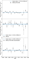 |
Fig. 1 Light curves of HESS J1745-290 and DE. Black markers indicate fitted fluxes for each calendar year. Vertical error bars show the statistical error on the fitted flux for that year. Horizontal error bars indicate the span of the observations within each year. The blue line represents the statistical mean of the light curve, with flux uncertainties accounted for, and the band represents the uncertainty on this value. Top: Raw HESS J1745-290 light curve. Middle: DE light curve. Bottom: Recalibrated HESS J1745-290 light curve. |
5 Sensitivity to time variations
5.1 General method
Our analysis indicates that the flux of HESS J1745-290 shows no significant variability. Here, we assess whether our dataset is sensitive to several theoretical scenarios that produce a time-dependent signal. A sensitivity study of this kind allows us to quantitatively rule out theoretical scenarios of source variability. For a variable source, this method can provide insight into the intrinsic behavior driving its variability.
To test the detectability of a given scenario, we simulated data cubes based on a theoretical source model (one for each year, depending on the time evolution scenario) using the simulation feature of Gammapy. We generated model predictions by convolving the models with the IRFs, and the resulting predicted counts were sampled assuming Poisson statistics to produce simulated observations that include noise. By repeating this sampling and model-fitting procedure several hundred times and averaging, we tested whether the measured result was compatible with the model within the uncertainties of the fitted model parameters.
In the following subsections, we describe tests of two types of theoretical variation: a one-off variation over a year relative to a constant flux value, and a linear negative variation over 16 years, as predicted by the model of Guo et al. (2013).
5.2 Overall sensitivity to yearly variations
The first test uses a constant hypothesis for the flux of HESS J1745-290. Its aim is to find the range of variation within which we cannot distinguish variation from statistical noise of a constant flux (for a 95% confidence interval of sensitivity, corrected for the 16 trials). Thus, even without evidence for the variation of HESS J1745-290, we can estimate the minimum variation rate that we can expect to detect, given our data and instrument. In practice, we used one dataset for each year, all with the same model;we simulated the data cubes 500 times, and then fit our previous 3D model onto the simulated maps, with only the normalizations free to vary. We obtained a Gaussian distribution of simulated HESS J1745-290 fluxes for each year, which we used to extract the 95% confidence range of fluctuations of the multi-year flux (then corrected for the number of trials). Figure 2 displays these results. The smallest of these ranges provides a lower bound on the sensitivity to deviations from a constant solution over this period. From our study, this minimal sensitivity is estimated to be around 27% (see Figure 2). This indicates that, given the time span of the H.E.S.S. observations of HESS J1745-290, we cannot expect to detect any significant flux variation smaller than 27% in a given year, even during the most sensitive year.
Tested evolution scenarios with corresponding χ2/degrees of freedom.
5.3 Sensitivity to particle injection from century-old Sgr A⋆ flares
Here we test an alternative scenario: a steady phenomenon as the origin of a linear temporal variation of the flux of HESS J1745-290. Motivated by the models of Chernyakova et al. (2011) and Guo et al. (2013) (see the discussion in 6.3), we tested the hypothesis that the TeV flux of HESS J1745-290 decreases linearly due to the evolution of a particle population injected during the massive, century-old flares of Sgr A⋆. To test the detectability of a linear temporal variation of HESS J1745-290’s flux, we simulated light curves to determine above which slope they display a significant linear variation of the γ-ray flux compared to a constant flux scenario. As before, we simulated the yearly datasets assuming different time-varying models to generate approximately 10 000 simulated light curves for each scenario. We tested linear decreases in flux of 0, 10, 20, 30, or 40% over 16 years. For each light curve, we tested the compatibility of a linear scenario and a constant scenario using a χ2 test. If the difference in χ2 exceeded (>3σ), the linear model provides a significantly better fit than the constant model, which we interpreted as a significantly detected variation. At the statistical level, we assessed how often a specific theoretical variation scenario produces a light curve with significant variation. We assumed that if a scenario produced a significantly observed variation in more than 68% of the simulations, it would have caused a significant variation within the H.E.S.S. dataset.
Figure 3 illustrates the results. The top panel shows the distribution of fitted linear variations for the five theoretical intrinsic linear flux decreases. We distinguish between “observed” light curves for which the linear model is preferred and those in which it is not. On average, the simulated variations follow the theoretical value (blue distributions, centered on the dashed black lines). However, if one considers only the detected variations, we see a bias toward higher values (the orange distributions are not centered on the dashed lines). This is due to a threshold below which H.E.S.S. cannot detect a 16-year linear variation. The bias decreases for larger theoretical variations (roughly over 40%). Hence, this confirms that, given the sensitivity of the H.E.S.S. dataset, any detected variability is associated with a real variation in the source flux. The bottom panel of Figure 3 quantifies the percentage of detected variations among the trials, as illustrated in the top panel. It shows, given a theoretical variation of the HESS J1745-290 source, the percentage of light curves that exhibit a significant linear decrease. The detection limit corresponds to a decrease of –28% (corresponding to –1.75% of the flux decrease per year), which rules out any larger flux variation over the last 16 years. This analysis confirms that testing a variation hypothesis over the entire period, rather than a single year, enables the detection of much smaller year-to-year variations. In the next section, we discuss the implications of these results for various emission scenarios.
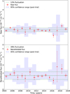 |
Fig. 2 Post-trial 95% confidence ranges of HESS J1745-290 flux per year (blue) when simulations assume a constant flux (solid green line). Top: raw source measurements. Bottom: recalibrated flux. The ranges are corrected for the number of trials. Data points from the analysis are shown in red in both panels. |
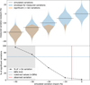 |
Fig. 3 Top: results of the simulated linearly varying source. Each violin plot shows the distribution of detectable variations over 16 years for each simulated intrinsic variation (from 0 to –40%; a dashed black line indicates that the mean of this distribution equals the simulated value). The full distribution is shown in blue, and the distribution of detected variations that are significantly preferred to a constant solution is shown in orange. Bottom: percentage of simulated light curves exhibiting a significant linear variation over 16 years compared to a constant flux model, as a function of simulated source flux linear variation. This percentage increases with the amplitude of the variation, reaching 68% (dashed blue line) for a simulated linear variation of –28% (corresponding to a flux decrease of –1.75% per year over 16 years). The shaded region represents values of simulated linear variations that induce a detectable variation (at the 3σ confidence level) with a probability greater than 68%. The best-fit linear variation actually observed on the data (though not significantly) is shown by the red line. |
6 Discussion
Particles accelerated in the inner accretion flow are expected to escape and propagate in the ISM surrounding Sgr A⋆, particularly within the 1.5-pc radius CND. Flux variations in the γ-ray emission are therefore modulated by the γ-ray production timescale, which depends on particle transport and matter distribution. Variability of HESS J1745-290 could therefore occur on timescales of months and years following a possible change in particle injection.
6.1 Yearly variation as a result of a transient event
The sudden change in particle injection and acceleration in the accretion flow could result from transient phenomena near Sgr A⋆, which would imply a rapid modification of the SMBH accretion rate. For instance, the model of Cuadra et al. (2015) shows how objects falling into the accretion flow can alter the luminosity of Sgr A⋆. In 2013–2014, an object known as G2 passed its pericenter around Sgr A⋆ (Witzel et al. 2014). The passage of this G2 object was quickly proposed as a potential trigger for such a phenomenon, as observed by Murchikova & Witzel (2021), and has motivated searches for visible counterparts of the SMBH activity. Notably, Chandra and XMM-Newton have detected a change in the bright X-ray flare rate since 2013 (Ponti et al. 2015; Mossoux & Grosso 2017; Mossoux et al. 2020). Although X-ray flares continue at a regular pace, the proportion of brighter flares has increased since that time. Although the overall X-ray flare has remained constant over two decades, (Mossoux et al. 2020) find that the rate of the brightest X-ray flares increased by a factor of 2.5 after mid-2014, suggesting a change in the activity of Sgr A⋆. However, the link between this evolution of Sgr A⋆’s X-ray activity and the G2 passage is doubtful, since the G2 object appears to be only one of many similar objects orbiting close to Sgr A⋆ around that time, and thus its influence on the SMBH was likely much smaller than initially suspected (Bouffard et al. 2019). However, analyses of X-ray flares monitored by Swift (Andrés et al. 2022) have also shown a higher activity of Sgr A⋆ in 2006–2007 and 2017– 2019 compared to 2008–2012, although Swift could not monitor the GC between 2013 and 2016 due to a nearby transient X-ray source. Assuming that matter fell towards Sgr A⋆ and altered the accretion flow, and assuming that the particle acceleration rate is proportional to the accretion rate, the TeV emission of the GC could be affected on comparable timescales, provided the radiation timescale is small. We tested the presence of any such significant variation in TeV luminosity before and after 2013 on an annual baseline, but we did not see any indication that the TeV emission seen by H.E.S.S. was altered around or after this year at this magnitude. However, we note that the overall fluence of the bright flares they considered (a few 1040 erg in a year) is small compared to the total fluence of Sgr A⋆ over a comparable period. Furthermore, the TeV emission may include contributions from both the inner accretion flow of Sgr A⋆ and the surrounding medium due to escaping particles, implying that even sudden and large variations in the accretion rate, directly traced by X-ray flares, could be significantly diluted and contribute only modestly to the measured TeV flux.
6.2 Long-term evolution of the accretion rate
We now consider the possibility that a long-term change in the injection and acceleration regime in the accretion disk of Sgr A⋆ could have occurred over the last decades, gradually affecting the amplitude of the TeV emission over the last 16 years. Testing these aspects is particularly interesting because while small short-term variations are limited by the H.E.S.S. sensitivity, extending the monitoring time of the GC over several years allows stronger constraints on long-term variations. Recently, a study of sub-millimeter data involving multiple instruments and their surveys of Sgr A⋆ over 20 years (Murchikova & Witzel 2021), found the variability of the mean flux to be approximately ±10% of the 14-year average (2005–2019). More recently, a 20% increase was measured in 2019 compared to the previous epoch (2015–2017) (GRAVITY Collaboration 2020; Boyce et al. 2022; Weldon et al. 2023). In this study, the averaged submillimeter fluxes are associated with a population of thermal electrons and are expected to vary together with the mean accretion rate of Sgr A⋆ (Yuan & Narayan 2014). Although we cannot yet place a constraining limit on this level of variation, our analysis excludes the possibility of a specific increase of flux in 2019 greater than 27%.
6.3 Remnants of major past bursts of Sgr A⋆
There are also indications that Sgr A⋆ itself was considerably more active in the recent past. The evolution of a large population of accelerated particles injected during the massive, century-old flares of Sgr A⋆ (Chuard et al. 2018) could also cause a long-term variation of the TeV emission, as suggested by Chernyakova et al. (2011) and Guo et al. (2013). X-ray surveys of nearby clouds in the central molecular zone show temporal brightness variations, particularly in the Fe Kα line, which have been explained as echoes of several moderately distant and very bright events (Clavel et al. 2013; Churazov et al. 2017; Chuard et al. 2018). This increase was interpreted as a considerable increase in X-ray activity at the GC (105 times the current luminosity) about one to two hundred years ago. Several authors have proposed that this implies that a large number of cosmic rays were accelerated at that time and have since been diffusing away from Sgr A⋆ into the ISM (Chernyakova et al. 2011; Guo et al. 2013). In this case, the resulting VHE γ-ray emission should decrease with time on a timescale dependent on the diffusion model, but likely on the order of decades or longer. As the initially accelerated CRs diffuse away into the ISM, their density near Sgr A⋆ decreases as ∼t−3/2 after a certain amount of time2. If most of the VHE γ rays result from the interaction of the CRs with the circumnuclear ring (as suggested by Linden et al. (2012)), then the resulting TeV emission should be roughly proportional to the CR density in the central few parsecs around the SMBH, following F(t) = F0t−3/2, where t is the time elapsed since the powerful flare, and F0 is the reference flux. The ratio between the flux at times t1 < t2 is then  . According to Churazov et al. (2017) and Chuard et al. (2018), a flaring event approximately 100–200 years ago can explain the X-ray echoes detected across the CMZ. For our window of observation, ∆t = 16 years, and assuming a powerful injection 100 years ago (from 2004), the relative decrease in TeV flux over the 16 years should be on the order of 20%. If we instead consider a 200-year-old flare, this relative decrease drops to 11%. According to our results, H.E.S.S. is not yet sensitive to such a resulting decrease in TeV flux over the last 16-years.
7 Conclusion
In this work, we analyze the data collected by H.E.S.S. on HESS J1745-290 between 2004 and 2019, making it the longest data set on this region at TeV energies. This work represents the first application of spectro-morphological analysis to H.E.S.S. observations of the Galactic center region. The updated spectrum of HESS J1745-290 is compatible with the spectrum previously published in (H.E.S.S. Collaboration 2016). We searched for variability in the flux of HESS J1745-290 flux on a yearly basis. We considered the variability of the central source with respect to the DE by recalibrating the yearly flux of HESS J1745-290 with the DE flux. We adopted this procedure to mitigate any residual time dependent systematic effects which could affect a 16-year-long survey.
As a result, this new study of the GC with H.E.S.S. finds that the central source HESS J1745-290 appears to be stable during this period, corroborating the recent findings of MAGIC (Ahnen et al. 2017) and VERITAS (Adams et al. 2021). A sensitivity study shows that our observations rule out year-to-year luminosity variations larger than 27% and linear decays larger than 28%, over the whole time range. Our constraints on a hypothetical variability of the central source show that the sensitivity of the instrument to a flux variation (i.e., its capability to detect a flux variation given a certain level of systematics) is not sufficient to rule out a number of time-evolution scenarios for the source. Hence, future monitoring of the Galactic center by CTA, with its enhanced sensitivity and improved control of systematics, should help to better constrain HESS J1745-290’s temporal behavior.
References
- Abdalla, H., Aharonian, F., Ait Benkhali, F., et al. 2021, A&A, 653, A152 [NASA ADS] [CrossRef] [EDP Sciences] [Google Scholar]
- Acero, F., Aharonian, F., Akhperjanian, A. G., et al. 2010, MNRAS, 402, 1877 [NASA ADS] [CrossRef] [Google Scholar]
- Adams, C. B., Benbow, W., Brill, A., et al. 2021, ApJ, 913, 115 [NASA ADS] [CrossRef] [Google Scholar]
- Aharonian, F., Akhperjanian, A. G., Aye, K. M., et al. 2004, A&A, 425, L13 [NASA ADS] [CrossRef] [EDP Sciences] [Google Scholar]
- Aharonian, F., Akhperjanian, A. G., Aye, K. M., et al. 2005, A&A, 432, L25 [NASA ADS] [CrossRef] [EDP Sciences] [Google Scholar]
- Aharonian, F., Akhperjanian, A. G., Bazer-Bachi, A. R., et al. 2006a, Phys. Rev. Lett., 97, 221102 [NASA ADS] [CrossRef] [Google Scholar]
- Aharonian, F., Akhperjanian, A. G., Bazer-Bachi, A. R., et al. 2006b, Nature, 439, 695 [Google Scholar]
- Aharonian, F., Akhperjanian, A. G., Bazer-Bachi, A. R., et al. 2006, A&A, 457, 899 [NASA ADS] [CrossRef] [EDP Sciences] [Google Scholar]
- Aharonian, F., Akhperjanian, A. G., Barres de Almeida, U., et al. 2008, A&A, 492, L25 [NASA ADS] [CrossRef] [EDP Sciences] [Google Scholar]
- Aharonian, F., Akhperjanian, A. G., Anton, G., et al. 2009, A&A, 503, 817 [NASA ADS] [CrossRef] [EDP Sciences] [Google Scholar]
- Ahnen, M. L., Ansoldi, S., Antonelli, L. A., et al. 2017, A&A, 601, A33 [CrossRef] [EDP Sciences] [Google Scholar]
- Albert, J., Aliu, E., Anderhub, H., et al. 2006, ApJ, 638, L101 [NASA ADS] [CrossRef] [Google Scholar]
- Andrés, A., van den Eijnden, J., Degenaar, N., et al. 2022, MNRAS, 510, 2851 [CrossRef] [Google Scholar]
- Archer, A., Barnacka, A., Beilicke, M., et al. 2014, ApJ, 790, 149 [Google Scholar]
- Archer, A., Benbow, W., Bird, R., et al. 2016, ApJ, 821, 129 [Google Scholar]
- Baganoff, F. K., Bautz, M. W., Brandt, W. N., et al. 2001, Nature, 413, 45 [Google Scholar]
- Ballantyne, D. R., Melia, F., Liu, S., & Crocker, R. M. 2007, ApJ, 657, L13 [Google Scholar]
- Ballantyne, D. R., Schumann, M., & Ford, B. 2011, MNRAS, 410, 1521 [NASA ADS] [Google Scholar]
- Becherini, Y., Punch, M., & H. E. S. S. Collaboration 2012, in American Institute of Physics Conference Series, 1505, High Energy Gamma-Ray Astronomy: 5th International Meeting on High Energy Gamma-Ray Astronomy, eds. F. A. Aharonian, W. Hofmann, & F. M. Rieger, 741 [NASA ADS] [Google Scholar]
- Berge, D., Funk, S., & Hinton, J. 2007, A&A, 466, 1219 [CrossRef] [EDP Sciences] [Google Scholar]
- Bouffard, É., Haggard, D., Nowak, M. A., et al. 2019, ApJ, 884, 148 [NASA ADS] [CrossRef] [Google Scholar]
- Boyce, H., Haggard, D., Witzel, G., et al. 2022, ApJ, 931, 7 [NASA ADS] [CrossRef] [Google Scholar]
- Cash, W. 1979, ApJ, 228, 939 [Google Scholar]
- Chalme-Calvet, R., de Naurois, M., & Tavernet, J. P. 2014, arXiv e-prints [arXiv:1403.4550] [Google Scholar]
- Chernyakova, M., Malyshev, D., Aharonian, F. A., Crocker, R. M., & Jones, D. I. 2011, ApJ, 726, 60 [NASA ADS] [CrossRef] [Google Scholar]
- Christopher, M. H., Scoville, N. Z., Stolovy, S. R., & Yun, M. S. 2005, ApJ, 622, 346 [Google Scholar]
- Chuard, D., Terrier, R., Goldwurm, A., et al. 2018, A&A, 610, A34 [NASA ADS] [CrossRef] [EDP Sciences] [Google Scholar]
- Churazov, E., Khabibullin, I., Sunyaev, R., & Ponti, G. 2017, MNRAS, 465, 45 [Google Scholar]
- Clavel, M., Terrier, R., Goldwurm, A., et al. 2013, A&A, 558, A32 [NASA ADS] [CrossRef] [EDP Sciences] [Google Scholar]
- Cuadra, J., Nayakshin, S., & Wang, Q. D. 2015, MNRAS, 450, 277 [CrossRef] [Google Scholar]
- Deil, C., Boisson, C., Kosack, K., et al. 2017, in American Institute of Physics Conference Series, 1792, 6th International Symposium on High Energy Gamma-Ray Astronomy, 070006 [Google Scholar]
- Do, T., Witzel, G., Gautam, A. K., et al. 2019, ApJ, 882, L27 [NASA ADS] [CrossRef] [Google Scholar]
- Dodds-Eden, K., Sharma, P., Quataert, E., et al. 2010, ApJ, 725, 450 [NASA ADS] [CrossRef] [Google Scholar]
- Donath, A., Terrier, R., Remy, Q., et al. 2023, A&A, 678, A157 [NASA ADS] [CrossRef] [EDP Sciences] [Google Scholar]
- Eckart, A., Baganoff, F. K., Morris, M., et al. 2004, A&A, 427, 1 [NASA ADS] [CrossRef] [EDP Sciences] [Google Scholar]
- Genzel, R., Schödel, R., Ott, T., et al. 2003, Nature, 425, 934 [NASA ADS] [CrossRef] [Google Scholar]
- Genzel, R., Eisenhauer, F., & Gillessen, S. 2010, Rev. Mod. Phys., 82, 3121 [Google Scholar]
- GRAVITY Collaboration (Abuter, R., et al.) 2020, A&A, 638, A2 [NASA ADS] [CrossRef] [EDP Sciences] [Google Scholar]
- GRAVITY Collaboration (Abuter, R., et al.) 2021, A&A, 654, A22 [NASA ADS] [CrossRef] [EDP Sciences] [Google Scholar]
- Guo, Y.-Q., Yuan, Q., Liu, C., & Li, A.-F. 2013, J. Phys. G Nucl. Phys., 40, 065201 [Google Scholar]
- H.E.S.S. Collaboration (Abramowski, A., et al.) 2016, Nature, 531, 476 [Google Scholar]
- H.E.S.S. Collaboration (Abdalla, H., et al.) 2018, A&A, 612, A9 [NASA ADS] [CrossRef] [EDP Sciences] [Google Scholar]
- H. E. S. S. Collaboration (Aharonian, F., et al.) 2023, A&A, 672, A103 [NASA ADS] [CrossRef] [EDP Sciences] [Google Scholar]
- Hillas, A. M. 1985, in International Cosmic Ray Conference, 3, 19th International Cosmic Ray Conference (ICRC19), 445 [NASA ADS] [Google Scholar]
- Hinton, J. A., & Aharonian, F. A. 2007, ApJ, 657, 302 [NASA ADS] [CrossRef] [Google Scholar]
- Khelifi, B., Djannati-Ataï, A., Jouvin, L., et al. 2015, in International Cosmic Ray Conference, 34, 34th International Cosmic Ray Conference (ICRC2015), 837 [Google Scholar]
- Kistler, M. D. 2015, arXiv e-prints [arXiv:1511.01159] [Google Scholar]
- Kosack, K., Badran, H. M., Bond, I. H., et al. 2004, ApJ, 608, L97 [CrossRef] [Google Scholar]
- Linden, T., Lovegrove, E., & Profumo, S. 2012, ApJ, 753, 41 [Google Scholar]
- Liu, S., Melia, F., Petrosian, V., & Fatuzzo, M. 2006, ApJ, 647, 1099 [Google Scholar]
- MAGIC Collaboration (Acciari, V. A., et al.) 2020, A&A, 642, A190 [NASA ADS] [CrossRef] [EDP Sciences] [Google Scholar]
- Mohrmann, L., Specovius, A., Tiziani, D., et al. 2019, A&A, 632, A72 [NASA ADS] [CrossRef] [EDP Sciences] [Google Scholar]
- Mossoux, E., & Grosso, N. 2017, A&A, 604, A85 [NASA ADS] [CrossRef] [EDP Sciences] [Google Scholar]
- Mossoux, E., Finociety, B., Beckers, J. M., & Vincent, F. H. 2020, A&A, 636, A25 [NASA ADS] [CrossRef] [EDP Sciences] [Google Scholar]
- Murchikova, L., & Witzel, G. 2021, ApJ, 920, L7 [NASA ADS] [CrossRef] [Google Scholar]
- Neilsen, J., Markoff, S., Nowak, M. A., et al. 2015, ApJ, 799, 199 [NASA ADS] [CrossRef] [Google Scholar]
- Ohm, S., van Eldik, C., & Egberts, K. 2009, Astropart. Phys., 31, 383 [NASA ADS] [CrossRef] [Google Scholar]
- Parsons, R. D., & Hinton, J. A. 2014, Astropart. Phys., 56, 26 [Google Scholar]
- Ponti, G., De Marco, B., Morris, M. R., et al. 2015, MNRAS, 454, 1525 [NASA ADS] [CrossRef] [Google Scholar]
- Ponti, G., George, E., Scaringi, S., et al. 2017, MNRAS, 468, 2447 [NASA ADS] [CrossRef] [Google Scholar]
- Roy, A., Gupta, A. C., Chitnis, V. R., et al. 2023, ApJS, 265, 14 [NASA ADS] [CrossRef] [Google Scholar]
- Schleicher, B., Arbet-Engels, A., Baack, D., et al. 2019, Galaxies, 7, 62 [NASA ADS] [CrossRef] [Google Scholar]
- Tsuboi, M., Handa, T., & Ukita, N. 1999, ApJS, 120, 1 [Google Scholar]
- Wang, Q. D., Lu, F. J., & Gotthelf, E. V. 2006, MNRAS, 367, 937 [NASA ADS] [CrossRef] [Google Scholar]
- Weldon, G. C., Do, T., Witzel, G., et al. 2023, ApJ, 954, L33 [NASA ADS] [CrossRef] [Google Scholar]
- Witzel, G., Ghez, A. M., Morris, M. R., et al. 2014, ApJ, 796, L8 [NASA ADS] [CrossRef] [Google Scholar]
- Witzel, G., Martinez, G., Willner, S. P., et al. 2021, ApJ, 917, 73 [NASA ADS] [CrossRef] [Google Scholar]
- Yuan, F., & Narayan, R. 2014, ARA&A, 52, 529 [Google Scholar]
- Yuan, F., Quataert, E., & Narayan, R. 2003, ApJ, 598, 301 [Google Scholar]
This optical efficiency is derived from the observation of muon events with H.E.S.S.. Comparing this measurement to the expected amount of Cherenkov light detected provides an estimate of the optical throughput of the instrument (between 0 and 1)(Chalme-Calvet et al. 2014).
The TeV flux should initially rise as the injected protons propagate through the ISM to cover the dense clouds and then decrease with the local density of CR.
Appendix A Yearly energy fluxes of HESS J1745-290
Recalibrated yearly energy fluxes of HESS J1745-290.
Appendix B Spectral index variation
We investigated the possibility of energy-dependent time variability of HESS J1745-290. We performed a time-resolved 3D analysis where spectral indices as well as normalizations of the DE and HESS J1745-290 are left free to vary during the fit procedure, whereas the cut-off energy of HESS J1745-290 spectrum is kept constant. We can see on figure B.1, that it did not result in any significant variation.
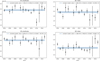 |
Fig. B.1 Evolution of the spectral index and normalization over time when left free to vary. Top: evolution of (left) the amplitude normalization and (right) spectral index of HESS J1745-290 with time. Bottom: evolution of (left) the amplitude normalization and (right) spectral index of the DE with time. In each panel, the blue line shows the best-fit constant value with its associated uncertainty. The corresponding χ2/d.o.f. values are indicated, showing that in all cases the parameters are compatible with being constant. |
All Tables
All Figures
|
Fig. 1 Light curves of HESS J1745-290 and DE. Black markers indicate fitted fluxes for each calendar year. Vertical error bars show the statistical error on the fitted flux for that year. Horizontal error bars indicate the span of the observations within each year. The blue line represents the statistical mean of the light curve, with flux uncertainties accounted for, and the band represents the uncertainty on this value. Top: Raw HESS J1745-290 light curve. Middle: DE light curve. Bottom: Recalibrated HESS J1745-290 light curve. |
| In the text | |
|
Fig. 2 Post-trial 95% confidence ranges of HESS J1745-290 flux per year (blue) when simulations assume a constant flux (solid green line). Top: raw source measurements. Bottom: recalibrated flux. The ranges are corrected for the number of trials. Data points from the analysis are shown in red in both panels. |
| In the text | |
|
Fig. 3 Top: results of the simulated linearly varying source. Each violin plot shows the distribution of detectable variations over 16 years for each simulated intrinsic variation (from 0 to –40%; a dashed black line indicates that the mean of this distribution equals the simulated value). The full distribution is shown in blue, and the distribution of detected variations that are significantly preferred to a constant solution is shown in orange. Bottom: percentage of simulated light curves exhibiting a significant linear variation over 16 years compared to a constant flux model, as a function of simulated source flux linear variation. This percentage increases with the amplitude of the variation, reaching 68% (dashed blue line) for a simulated linear variation of –28% (corresponding to a flux decrease of –1.75% per year over 16 years). The shaded region represents values of simulated linear variations that induce a detectable variation (at the 3σ confidence level) with a probability greater than 68%. The best-fit linear variation actually observed on the data (though not significantly) is shown by the red line. |
| In the text | |
|
Fig. B.1 Evolution of the spectral index and normalization over time when left free to vary. Top: evolution of (left) the amplitude normalization and (right) spectral index of HESS J1745-290 with time. Bottom: evolution of (left) the amplitude normalization and (right) spectral index of the DE with time. In each panel, the blue line shows the best-fit constant value with its associated uncertainty. The corresponding χ2/d.o.f. values are indicated, showing that in all cases the parameters are compatible with being constant. |
| In the text | |
Current usage metrics show cumulative count of Article Views (full-text article views including HTML views, PDF and ePub downloads, according to the available data) and Abstracts Views on Vision4Press platform.
Data correspond to usage on the plateform after 2015. The current usage metrics is available 48-96 hours after online publication and is updated daily on week days.
Initial download of the metrics may take a while.