| Issue |
A&A
Volume 709, May 2026
|
|
|---|---|---|
| Article Number | A225 | |
| Number of page(s) | 8 | |
| Section | Astrophysical processes | |
| DOI | https://doi.org/10.1051/0004-6361/202556929 | |
| Published online | 19 May 2026 | |
A study of the diffusion mechanism in pulsar wind nebulae: Application to HESS J1420–607
1
College of Science, Yunnan Agricultural University, Kunming 650201, PR China
2
Department of Physics, Yuxi Normal University, Yuxi 653100, PR China
3
Department of Astronomy, Key Laboratory of Astroparticle Physics of Yunnan Province, Yunnan University, Kunming 650091, PR China
★ Corresponding authors: This email address is being protected from spambots. You need JavaScript enabled to view it.
; This email address is being protected from spambots. You need JavaScript enabled to view it.
Received:
21
August
2025
Accepted:
25
March
2026
Abstract
Aims. Recent studies have demonstrated the existence of slow diffusion phenomena in pulsar wind nebulae (PWNe), where the diffusion coefficient of particles is significantly smaller than the value considered to be the average in the Galaxy. We explored the particle slow diffusion mechanism in the frame of a time-dependent spatially uniform model that incorporates both particle advection and diffusion.
Methods. Based on the turbulence theory, we considered the gyroresonant interactions between the particles and turbulent waves, which enabled us to determine the diffusion coefficients of particles within nebulae via the turbulent scale and magnetic field components (ordered magnetic field and turbulent magnetic field). Meanwhile, by considering injection, advection, adiabatic loss, and radiative loss of particles, the multiband nonthermal emission from a PWN was produced by the relativistic leptons through synchrotron radiation and inverse Compton process.
Results. The diffusion coefficient increases with the turbulent scale, whereas it decreases with the turbulent-to-ordered magnetic field strength ratio. Meanwhile, effects of the turbulent scale and magnetic field components on spectral energy distributions (SEDs) were analyzed. This model was applied to HESS J1420−607, and the observed spectral energy distribution of photon emission was reproduced well. The results suggest that (1) the particle cooling processes are dominated by adiabatic loss in lower-energy bands, and synchrotron loss dominate for the higher-energy particles, and (2) the advection is the most prominent process to particle transport within this nebula, and the diffusion only plays a role in the high-energy band. More importantly, our model estimates the current diffusion coefficient at an electron energy of 1 TeV 5.69 × 1026 cm2 s−1, and the slow diffusion mechanism may arise from the small-scale turbulence and a relatively strong turbulent magnetic field in HESS J1420−607.
Key words: radiation mechanisms: non-thermal / pulsars: general / stars: winds / outflows
© The Authors 2026
 Open Access article, published by EDP Sciences, under the terms of the Creative Commons Attribution License (https://creativecommons.org/licenses/by/4.0), which permits unrestricted use, distribution, and reproduction in any medium, provided the original work is properly cited.
This article is published in open access under the Subscribe to Open model. This email address is being protected from spambots. You need JavaScript enabled to view it. to support open access publication.
1. Introduction
Pulsar wind nebulae (PWNe) are outflows of relativistic particles powered by the center rotational pulsar, and they generally emit photons from radio to gamma-ray energies (Kennel & Coroniti 1984; Gaensler & Slane 2006). In particular, the Fermi-Large Area Telescope (LAT), the H.E.S.S. Galactic Plane Survey (HGPS), and the Large High Altitude Air Shower Observatory (LHAASO) detected many PWNe in the very high-energy (VHE) and ultra-high-energy (UHE) gamma-ray bands (e.g., The Fermi-LAT Collaboration 2025; H.E.S.S. Collaboration 2018a; Cao et al. 2021a,b, 2024). Numerous observations reveal that PWNe are strong candidates for Galactic PeVatrons. Detecting the broadband spectral energy distributions (SEDs) of Galactic sources is critical to investigating the nonthermal radiation properties of particles within PWNe.
It is generally believed that the radio and X-ray emission from PWNe are produced by the synchrotron radiation, and the γ-rays are generated by the inverse Compton (IC) scattering processes of the relativistic electrons (e.g., Kennel & Coroniti 1984; Zhang et al. 2008; Fang & Zhang 2010; Tanaka & Takahara 2010; Bucciantini et al. 2011; Martín et al. 2012; Torres et al. 2014; Lu et al. 2017; van Rensburg et al. 2018; Zhu et al. 2018, 2021; Lu et al. 2023b). The γ-ray emission also appears to be produced by the decay of neutral pions in the proton-proton interaction of energetic nucleons with the ambient interstellar medium (Atoyan & Aharonian 1996; Zhang & Yang 2009; Liu & Wang 2021; Nie et al. 2022; Peng et al. 2022). Theoretically, these relativistic particles are injected at the termination shock and then transported away from the center of the nebula. However, the transport mechanism and origin of these particles are still debated.
In the transport view, the particle transport mainly includes convection and diffusion processes (e.g., Vorster & Moraal 2013; Van Etten & Romani 2011; Tang & Chevalier 2012; Porth et al. 2016; Lu et al. 2017; Zhu et al. 2021, 2023; Martin et al. 2024). The importance of the particle advection process within PWNe has been described in some previous studies (Rees & Gunn 1974; Kennel & Coroniti 1984). However, the particle advection form is still highly debated for PWNe. On the other hand, the diffusion process was first proposed within PWNe (Gratton 1972; Wilson & Shakeshaft 1972). The diffusion coefficient of particles within PWNe is generally believed to be dependent on the structure of the magnetic field and the energy of the particles (Lerche & Schlickeiser 1981; Caballero-Lopez et al. 2004). Numerous theoretical studies have also shown that the particle diffusion mainly originates from turbulent processes, and means that the turbulence is certainly crucial for exploring the particle transport within PWNe (e.g., Bucciantini et al. 2011; Porth et al. 2014, 2016; Lu et al. 2023b, 2024). Moreover, some observational evidence of turbulence in PWNe have been recently presented (e.g., Shibata et al. 2003; Bucciantini et al. 2023; Mizuno et al. 2023; Deng et al. 2024). However, the nature of the turbulence magnetic fields is still unknown.
Furthermore, to explain the observed nonthermal radiation properties within PWNe, a significantly small diffusion coefficient is needed (e.g., Yüksel et al. 2009; Lu et al. 2017; Abeysekara et al. 2017; Zhu et al. 2021, 2023). To date, the origin of such a slow diffusion zone is still unclear. For example, López-Coto & Giacinti (2018) have shown that a small turbulence scale may produce the slow diffusion coefficient; Evoli et al. (2018) suggested the self-generated turbulence caused by relativistic electrons flow restricting the diffusion of relativistic electrons; and Fang et al. (2019) considered the constraint of diffusion from the strong turbulence generated by the shock wave of the parent supernova remnant.
Currently, these multiband nonthermal radiative property studies are mainly divided into two categories: the spatially uniform model and the spatially dependent model. In the spatially uniform model, the nebula is assumed to be filled with relativistic particles with an averaged distribution, and the magnetic field, particle radiation and transport processes are homogeneous throughout the region (e.g., Atoyan & Aharonian 1996; Zhang et al. 2008; Zhang & Yang 2009; Fang & Zhang 2010; Tanaka & Takahara 2010; Meyer et al. 2010; Bucciantini et al. 2011; Martín et al. 2012; Torres et al. 2014; Liu & Wang 2021; Zhu et al. 2021; Nie et al. 2022; Lu et al. 2023b; Martin et al. 2024). In contrast, these physical processes and parameters vary spatially in the spatially dependent model (e.g., Kennel & Coroniti 1984; Van Etten & Romani 2011; Vorster & Moraal 2013; Porth et al. 2016; Lu et al. 2017; van Rensburg et al. 2018; Peng et al. 2022). Although the spatially uniform model is an over-simplification, it has been and is still being widely used.
With motivation from both the slow diffusion found in observations and theoretical predictions of turbulent diffusion. In this paper, we use a time-dependent spatially uniform model with particle advection and diffusion to investigate the effects of particle turbulent on multiband nonthermal radiative properties of pulsar wind nebulae. The rest of the paper is organized as follows. In Sect. 2 the details of the model are described. The model application results on the nebula are presented in Sect. 3. Finally, our summary and discussion are presented in Sect. 4.
2. Model description
We assume that the energy of PWN is injected from the pulsar within the nebula. In addition, the evolution of the spin-down luminosity is given by (Pacini & Salvati 1973; Gaensler & Slane 2006)
 (1)
(1)
where L0 is the initial luminosity, and τ0 is the initial spin-down timescale. Most measured values for the braking index n have been found between 2 and 3 (Gaensler & Slane 2006; Ou et al. 2016), but typically n = 3 is assumed in this work. This would indicate a pure magnetic dipole radiation on the pulsar’s surface. The initial spin-down timescale, τ0, is given by
 (2)
(2)
where τc is the characteristic age of the pulsar,
 (3)
(3)
where P and Ṗ are the period and period derivative of pulsar. In addition, the current spin-down luminosity, L(tage), can be calculated by
 (4)
(4)
where I is the moment of inertia of the pulsar, which is adopted to be 1045 g cm2 in this paper. We note that the tage is the age of the PWN. If t = tage and n are given, the L0 and τ0 can be obtained.
In general, the spin-down luminosity L(t) is injected into PWN, and distributed between particles of energy and the magnetic field energy (Rees & Gunn 1974; Kennel & Coroniti 1984; Gaensler & Slane 2006; Gelfand et al. 2009). In this paper, as in Tanaka & Ishizaki (2024), the injection term is modified by involving a particle perturbation process. Thus, the energy injection rate is given by
 (5)
(5)
where ηB + ηe + ηT = 1. Here Ėe(t) = ηeL(t) represents the injection rate of particle energy, ĖB(t) = ηBL(t) represents the injection rate of ordered magnetic field, and ĖT(t) = ηTL(t) represents the injection rate of turbulent component energy. Compared with the previous model, we have introduced the turbulent components, which are continuously supplied from the central pulsar.
Assuming spherical symmetry, the evolution of the particles within PWNe can be described as (Zhu et al. 2021, 2023)
![Mathematical equation: $$ \begin{aligned} \frac{\partial N(E,t)}{\partial t}= \frac{\partial }{\partial E} \left[\dot{E} N(E,t)\right] + \frac{N(E,t)}{\tau _{\rm con}(E,t)} + \frac{N(E,t)}{\tau _{\rm diff}(E,t)} + Q(E,t), \end{aligned} $$](/articles/aa/full_html/2026/05/aa56929-25/aa56929-25-eq6.gif) (6)
(6)
where Ė is the total energy loss of the particle, τcon is the advection timescale of particle, τdiff is the diffusion timescale of particle, and Q(E, t) is the injection term.
For the total energy loss Ė, it includes the adiabatic loss Ėad, synchrotron radiation loss Ėsyn, and inverse Compton scattering loss ĖIC. Thus, the total energy-loss Ė is written as
 (7)
(7)
where the adiabatic loss Ėad is given by (Tanaka & Takahara 2010)
 (8)
(8)
where VPWN is the expansion velocity, RPWN is the radius of nebula, and Ee is electron energy. Then the synchrotron cooling Ėsyn is given by (Rybicki & Lightman 1979)
 (9)
(9)
where σT is the Thomson cross section, and  is the total magnetic field energy density, i.e., the ordered magnetic field plus turbulent magnetic field energy density. Lastly, the inverse Compton cooling ĖIC is given by (Blumenthal & Gould 1970)
 (10)
(10)
where h is the Planck constant, νi and νf are respectively the initial and final frequencies of the scattered photons, H is the Heaviside step function, and n(νi) is the distribution of target photon fields. The function f(q, Γ) can be expressed as
 (11)
(11)
with Γ = 4hνi(Ee/mec2)/mec2 and q = hνf/Γ(Ee − hνf).
It is generally believed that the particle transport includes advection and diffusion processes. For the advection process, the advection velocity form is still unclear. According to PWN, the magnetohydrodynamic (MHD) simulations find that the radial velocity profile depends on the ratio of electromagnetic to particle energy, σ (Kennel & Coroniti 1984). When σ = 1, the velocity remains almost independent of r. When σ = 0.01, the velocity falls off as V(r)∝r−2. Therefore, in the current theoretical studies, it is usually assumed that V(r)∝r−γ, where 0 ≤ γ ≤ 2 (Schöck et al. 2010; Van Etten & Romani 2011; Holler et al. 2012; H.E.S.S. Collaboration 2019; Principe et al. 2020; Park et al. 2023; Collins et al. 2024). In our model, the nebular plasma is assumed to be a good conductor, and the ideal MHD equations are applied to describe the PWN wind, with the result that the magnetic field is frozen into the outflowing plasma. Thus, Ohm’s law becomes
 (12)
(12)
and combining Eq. (12) with Faraday’s law we obtain
 (13)
(13)
Meanwhile, similarly to Kennel & Coroniti (1984), Lu et al. (2017), Lu et al. (2023a), Zhu et al. (2023), Kundu et al. (2024), and Martin et al. (2024), we assumed that the temporal change of the B field is slow enough that we can set ∂B/∂t ≃ 0. Thus, an ideal MHD limit, VBr = constant, is obtained. As mentioned in Sect. 1, the magnetic field within the nebula is homogeneous for the spatially uniform model, and the advection velocity is assumed to be equal to the expansion velocity VPWN of the nebula at the outer boundary. Thus, the advection velocity can be approximated as (e.g., Zhu et al. 2021)
![Mathematical equation: $$ \begin{aligned} V(r) = V_{\rm PWN}(t) \left[\frac{R_{\rm PWN}(t)}{r}\right]. \end{aligned} $$](/articles/aa/full_html/2026/05/aa56929-25/aa56929-25-eq15.gif) (14)
(14)
Then the advection timescale of particles τcon is described as (Vorster & Moraal 2013)
 (15)
(15)
where Rts(t) is the radius of termination shock. Combining Eqs. (14) and (15), τcon is written as
 (16)
(16)
where τad = Ee/Ėad(Ee,t) is the adiabatic loss timescale.
On the other hand, the nature of the particle diffusion strongly depends on the distribution of the turbulent waves within the nebula, and a power-law form of spectral density of turbulent waves is assumed in the model (e.g., Miller et al. 1996; Elmegreen & Scalo 2004)
 (17)
(17)
where k and δ are the wave number and diffusion index. It was claimed that the diffusion index of 0.3 ≤ δ ≤ 0.6 could match CR observations in the Milky Way remarkably well (Strong et al. 2007; Trotta et al. 2011; Hopkins et al. 2022). The value of power law index δ depends on the property of turbulence in ambient medium, and the different values represent different diffusion forms, for example δ = 1/3 describes Kolmogorov-type turbulence (e.g., Kolmogorov 1941), and δ = 1/2 the Kraichnan-type turbulence (e.g., Kraichnan 1965). In this paper, motivated by the previous studies (e.g., Abeysekara et al. 2017; Tang & Piran 2019; Zhu et al. 2021, 2023), the particle diffusion is assumed as the typical Kolmogorov diffusion, i.e., δ = 1/3.
It is generally assumed that the turbulence is composed of Alfvén waves, its kinetic energy and magnetic energy of turbulent fluid would be equal (e.g., ωδB(k) = 0.5ω(k); Zhou & Matthaeus 1990; Miller & Roberts 1995). According to the conservation of energy, the normalization constant ω0 for the injection spectrum is determined by
 (18)
(18)
where uδB = δB2/8π is the energy density of the turbulent magnetic field, kmin is the minimum wavenumber of the injection turbulence waves, and kmax is the maximum wavenumber of the injection turbulence waves. Combining Eqs. (17) and (18) can be rewritten as
 (19)
(19)
and then, by integrating Eq. (19), the normalization constant ω0 is described as
 (20)
(20)
Here we note that the minimum and maximum turbulence wave number are related to the maximum and minimum scale of the turbulence Lmax and Lmin via kmin = 2π/Lmax and kmax = 2π/Lmin, respectively. Meanwhile, Lmin ≪ Lmax, which results in kmax ≫ kmin, and thus the spectral density of the turbulence waves is described by
 (21)
(21)
According to Harari et al. (2002), for a power-law magnetic power spectrum the turbulent correlation scale is evaluated as
 (22)
(22)
which gives Lc ≃ Lmax/5 in the case of a Kolmogorov-type turbulence. Here we note that the turbulent maximum scale Lmax cannot exceed the size of the nebula RPWN, while the turbulent correlation scale Lc should not be smaller than the gyro-radius of the particle in our model. For convenience, we assumed Lmax = κRPWN resulting in Lc ≃ 0.2κRPWN. It should be noted that the coherence length Lc is not sufficiently long within PWNe here. As a result, particles traverse multiple magnetic coherence lengths, leading to the overall turbulence becoming isotropic.
For the an arbitrary turbulence level, the diffusion coefficient is determined by the approximate equation (e.g., Skilling 1971; Ptuskin & Zirakashvili 2003, 2005)
 (23)
(23)
where  is the gyro-radius of electrons and ζ(kres) = kresω(kres)/(uB + uδB) is the ratio of the turbulence energy density at scale rg = 2π/kres to the average total magnetic energy density. Consistent with previous some studies, the average magnetic field strength is defined as the square root of the sum of the squares of the ordered and turbulent magnetic fields
  (e.g., Casse et al. 2001; Giacinti et al. 2018; Reichherzer et al. 2020). Thus, the coefficient is rewritten as
 (24)
(24)
Subsequently, the diffusion timescale of particles τdiff is described by (e.g., Parker 1965)
 (25)
(25)
Turbulence is composed of Alfvén waves, and so the kinetic energy and its magnetic energy of turbulent fluid would be equal. Thus, an indirect parameter  is introduced. For simplicity and consistency, the evolution of turbulent magnetic field and kinetic energy to be similar to that of Gelfand et al. (2009) for the ordered magnetic field term. Therefore, according to the conservation of energy, the ordered magnetic field and turbulent magnetic field in the nebula B(t), δB are calculated by
 (26)
(26)
The last term on the right-hand side of Eq. (6) is Q(E, t), which is usually assumed as a broken power law,
 (27)
(27)
where Q0(t) is a time-dependent normalization coefficient, Eb is the energy break, α1 and α2 are low- and high-energy spectral indices, respectively. Lastly, Emax is the maximum energy of the injected electrons and positrons. The time-dependent normalization coefficient Q0(t) can be estimated by
 (28)
(28)
Similarly to Gelfand et al. (2009), the dynamical properties can be self-consistently studied for the PWN. As mentioned in Gelfand et al. (2009), the large-scale evolution of a composite SNR depends on the mechanical energy of the explosion Esn, the density of the ambient medium ρISM, the mass of the supernova ejecta Mej, and the spin-down power of the pulsar L(t). The evolution of the SNR radius RSNR(t), the reverse shock radius Rrs(t), the PWN radius RPWN(t), and the termination shock radius Rts(t) of the system can be calculated. The calculation process here is the same as in Gelfand et al. (2009, for details, see their Sect. 2.2).
3. Model application
To calculate the SED of nonthermal photons, the particle spectra at the current time (N(E,t)) is obtained by solving the evolution equation of particles (Eq. (6)), and then the SEDs of nonthermal photons are calculated through synchrotron radiation and IC scattering of particles inside PWNe. It is emphasized that the average magnetic field, i.e.,  is applied during the radiation process.
3.1. Effects of turbulence scale and magnetic field components on the SEDs
As demonstrated in Eq. (24), the diffusion coefficient of a particle increases with the turbulent scale, whereas it decreases with the turbulent-to-ordered magnetic field ratio. It is generally suggested that the particle diffusion process has significantly modified the spectral energy distributions (SEDs) within PWNe (e.g., Zhu et al. 2021; Lu et al. 2023b, 2024). Therefore, the effects of the turbulence scale and magnetic field components on the SEDs of the PWN are researched here. We used the model parameters of the benchmark as follows: the pulsar and ejecta parameters are the same as those of HESS J1420−607 (whose values are listed in Table 1), and the adopted parameters are Eb = 1.0 × 10⁵ MeV, α1 = 1.5, and α2 = 2.5, and the maximum energy of particles, Emax = 1.0 PeV. Using the model described in Sect. 2, the corresponding SEDs are obtained through synchrotron radiation and the IC scattering of relativistic electrons and positrons. We note that the four soft photon fields are involved in the inverse Compton scattering: the cosmic microwave background (CMB), the galactic far-infrared (FIR) background, the near-infrared (NIR), and synchrotron radiation photon (SSC) fields. The related energy density and temperature are the same as those of HESS J1420−607 (for details, see below).
Values of physical parameters used for HESS J1420−607.
To study the effects of the particle turbulence scale on spectral energy distributions (SEDs), we assume the magnetic fraction ηB = 0.1 and the turbulence fraction ηT = 0.1, thereby excluding the influence of magnetic field components. We note that these two values imply the ratio  . As illustrated in the left panel of Fig. 1, the SEDs for different scales are calculated. Here, the different colored lines correspond to SEDs with varying ratios of injection scale to PWN radius. To ensure that the turbulent correlation scale cannot exceed the size of the nebula, and should not be smaller than the gyroradius of the maximum particle energy considered, we assumed the range of the ratio 0.01 < κ < 1.0. The results indicate that the SEDs of PWNe exhibit a strong dependence on the particle turbulence scale. Across all energy bands, the flux decreases with increasing κ. The main reason is that a large value of κ indicates a large diffusion coefficient (for details, see Eq. (24)), and fast diffusion leads to faster particle escape from the nebula.
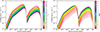 |
Fig. 1. Spectral energy distributions of the PWN. The different colored lines correspond to the SEDs for different values of κ (left panel) and δB/B (right panel). |
In addition, the effects of the magnetic field components (which include the turbulent magnetic field and ordered magnetic field) on the SEDs are also investigated. We note that the turbulent magnetic field and ordered magnetic field are mainly governed through ηB and ηT in the model. Meanwhile, to avoid the influence of injected particles and turbulence scale, we assumed that ηB + ηT = 0.2 and κ = 0.1. As demonstrated in Eq. (24), the diffusion coefficient decreases with the increase in the ratio of the turbulent magnetic field to the ordered magnetic field δB/B, while the increasing trend progressively weakens. As shown in the right panel of Fig. 1, the effects of the weak turbulent magnetic field (ηT = 0.004 and ηB = 0.196, corresponding ratio δB/B = 0.1) to relatively strong turbulent magnetic field (ηT = 0.189 and ηB = 0.011, corresponding ratio δB/B = 3.0) on the resulting nonthermal emission are investigated. The results show that the SEDs of PWNe depend on the ratio δB/B, and all the flux increases with increasing δB/B.
3.2. Application to HESS J1420–607
We now apply the model to pulsar wind nebulae HESS J1420−607, which is also known as K3 PWN. It is a TeV emission source detected in the HESS Galactic Plane survey (Manchester et al. 2005; H.E.S.S. Collaboration 2018b). Numerous observational studies have identified as originating from the PWN powered by PSR J1420−6048, which exhibits a spin period of P = 68.18 ms, a period derivative of Ṗ = 8.32 × 10⁻¹⁴ s s−1, a characteristic age τc ∼ 13 kyr, and a current spin-down luminosity of L(tage) = 1.04 × 1037 erg s−1 (D’Amico et al. 2001; Ng et al. 2005; Aharonian et al. 2006; Weltevrede et al. 2010). In addition, based on a dispersion measure model to estimate the distance of the pulsar d = 5.6 kpc (Ng et al. 2005; Weltevrede et al. 2010). For the age of the system, Park et al. (2023) assumed the age of Tage = 9000 yr based on the ratio of the γ-ray to X-ray flux (for details, see Kargaltsev et al. 2013). Consequently, using Eqs. (2) and (1), the initial spin-down timescale τ0 = 3.99 kyr and the initial luminosity L0 = 1.10 × 1038 erg s−1 are estimated.
To study the nonthermal radiative properties by spectral energy distribution (SED) of HESS J1420−607, we collected the multiband nonthermal observational data. The radio data are from Roberts et al. (1999) and Van Etten & Romani (2010), the X-ray data are from Van Etten & Romani (2010), the GeV Fermi-LAT data are from Tian et al. (2023), and the TeV data are from Aharonian et al. (2006). We note that Park et al. (2023) regarded the radio measurements of Van Etten & Romani (2010) and Roberts et al. (1999) as upper and lower limits, respectively. We also take these values as the lower and upper limit, respectively. Furthermore, the X-ray images have revealed the angular radius θX − ray ∼ 3.0′, which implied the corresponding radius RX − ray ∼ 4.9 pc for the distance of 5.6 kpc (Van Etten & Romani 2010). The Fermi-LAT measured the size of the PWN θGeV ∼ 0.12°, the corresponding radius RGeV ∼ 11.7 pc (Ackermann et al. 2017; Tian et al. 2023). In addition, the H.E.S.S. observations show the angular radius θTeV ∼ 0.08° and the corresponding radius RTeV ∼ 7.9 pc (H.E.S.S. Collaboration 2018a,b).
We applied the model to reproduce the multiwavelength SED of HESS J1420−607, and the results show the observed nonthermal spectrum can be well reproduced through synchrotron radiation and IC scattering of relativistic electrons and positrons. In our calculation, the target photons consist of three components: the cosmic microwave background (CMB) photons, the galactic near-infrared (NIR) photons, and far-infrared (FIR) photons. The energy densities of far-infrared (FIR) photons UIR = 3.0 eV cm−3 and the corresponding temperatures TIR = 10 K are applied. The galactic near-infrared (NIR) photons UNIR = 2.0 eV cm−3 and the corresponding temperatures TNIR = 3500 K (Van Etten & Romani 2010) are also used in the calculation. It should be noted that the UIR value we used is higher than the Galactic average dust emission. In fact, the target photon energy densities are generally higher than the values obtained from the GALPROP code based on the position of the source in the Galaxy (Torres et al. 2014). To reproduce the observed SEDs, the values of pulsar and SN parameters are generally measured or assumed. As in some previous studies (Zhu et al. 2023, 2024), the low-energy spectral index α1, high-energy index α2, energy break Eb, magnetic fraction ηB, turbulence field fraction ηT, ratio of the turbulence maximum scale to PWN radius κ, and maximum energy of particles Emax are considered as fitted parameters. In the fitting process, the Levenberg-Marquardt (LM) method of the χ2 minimization fitting procedure (Press et al. 1992) is used to obtain the best-fitting values and their uncertainties. These values and the reduced χ2 values are also reported in Table 1. We note that, given the limited quality of the observational data, some fitted parameter uncertainties are large. As shown in Table 1, α1 = 1.54, α2 = 2.71, Eb = 2.09 × 10⁶ MeV, ηB = 0.015, ηT = 0.319, κ = 0.031, and Emax = 0.54 PeV; these fitting results are similar to those values previously obtained in typical PWNe (Torres et al. 2014; Zhu et al. 2018, 2023).
The results of the SED calculated and the corresponding timescales considered are shown in Fig. 2. The left panel of Fig. 2 shows that the multiband data are reproduced well by synchrotron and IC emission of relativistic electrons and positrons. The right panel of Fig. 2 shows that the effects of the cooling mechanisms are dominated by adiabatic loss for Ee < 1.2 × 10⁷ MeV, the IC scattering losses dominate over the synchrotron loss and adiabatic loss for 1.2 × 10⁷ < Ee < 1.3 × 10⁸ MeV, and the synchrotron loss dominates over the adiabatic loss and IC scattering losses for Ee > 1.3 × 10⁸ MeV. On the other hand, particle transport dominated by advection for Ee < 2.9 × 10⁷ MeV, and the effect of diffusion increases with the increase of energy. Lastly, the diffusion becomes the dominant process for Ee > 2.9 × 10⁷ MeV. In fact, previous studies found that advection-dominated transport of particles for low-energy bands, and the diffusion becomes the dominant process for high-energy bands within some PWNe (Zhu et al. 2021; Lu et al. 2023a; Zhu et al. 2023).
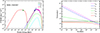 |
Fig. 2. Left panel: Comparison of calculated multiband SEDs with the observed data for HESS J1420−607. The dark cyan and purple data points display radio measurements from Roberts et al. (1999) and Van Etten & Romani (2010). The olive points show X-ray measurements (Van Etten & Romani 2010), the blue and magenta points respectively represent the Fermi-LAT data (Tian et al. 2023) and H.E.S.S. measurements (Aharonian et al. 2006). The black dashed line represents synchrotron SED; the blue, green, and dark yellow dashed lines represent the SEDs of inverse Compton scatterings with the IR, CMB, and starlight, respectively. Right panel: Different cooling and propagation timescales at the current time. The solid back, magenta, blue, green, dark yellow, and red lines represent the adiabatic loss timescale, synchrotron cooling timescale, inverse Compton cooling timescale, diffusion timescale, advection timescale, and total timescale, respectively. |
In addition, our multiband nonthermal emission modeling indicated that particles are accelerated to ∼0.6 PeV energy, which implies the HESS J1420−607 is a Galactic PeVatron candidate. Meanwhile, the radius of 11.8 pc was obtained, which is consistent with the PWN-measured size in the GeV-band (Ackermann et al. 2017; Tian et al. 2023). We further found the ordered magnetic field strength B = 2.25 μG, the turbulent magnetic field strength B = 7.41 μG, and the ratio δB/B ∼ 3.3. These values reveal that turbulence magnetic field within HESS J1420−607 is relatively strong. Additionally, in our model calculation, the ratio of injection scale to PWN radius is κ = 0.031. It implies the turbulence correlation scale Lc ≃ 0.073 pc. Compared with the typical gyro-radius of particles,  , which implies the maximum gyro-radius rg, max ≃ 0.07 pc, the turbulence correlation scale Lc is larger than the gyro-radius of particle. In fact, the coherence length Lc is significantly smaller than the typical coherence length of the interstellar magnetic field, lc, which lies in the range ∼1−200 pc (Haverkorn et al. 2008; Cho & Ryu 2009; Chepurnov & Lazarian 2010; Beck et al. 2016).
We also obtained the current diffusion coefficient ∼5.69 × 1026 cm2 s−1 at the electron energy of 1 TeV. The result is consistent with previous studies, i.e., the slow-diffusion mechanism may exist within PWNe (Lu et al. 2017; Abeysekara et al. 2017; Zhu et al. 2021, 2023). To date, the open question is the possible physical origin of such a slow diffusion mechanism. A possibility suggested in some previous studies is that some pulsars can be located in regions with a much higher turbulence level than the average ISM (e.g., Fang et al. 2019; Vieu & Reville 2023). Another possible explanation is that a small turbulence scale may produce the slow diffusion (López-Coto & Giacinti 2018; Amato & Recchia 2024). In our model, as presented in Eq. (24), we considered that the slow diffusion mechanism may originate from both small-scale turbulence and relatively strong turbulence magnetic field distribution.
4. Conclusion and discussions
In recent years, some studies have found that turbulence process can play a major role for investigating the diffusion of particle within PWNe (Bucciantini et al. 2011; Porth et al. 2014, 2016; Lu et al. 2023b, 2024). Furthermore, some studies suggest that PWNe may have a strong turbulent magnetic field (Porth et al. 2014, 2016; Lyutikov et al. 2019; Luo et al. 2020; Bucciantini et al. 2023). In this paper, for the first time, a spectral evolution model involving the turbulence-induced particle diffusion, advection, and cooling processes is presented. When compared to previous models (e.g., Zhang et al. 2008; Bucciantini et al. 2011; Martín et al. 2012; Torres et al. 2014; Zhu et al. 2018, 2021; Fiori et al. 2022), this model enabled us to understand the mechanism of particle diffusion within nebulae.
Based on the turbulence theories, as shown in Eq. (24), the diffusion coefficient of a particle within the nebula was determined by the turbulence scale and magnetic field components (ordered magnetic field and turbulent magnetic field). Furthermore, the effects of the turbulence scale and the turbulent-to-ordered magnetic field strength ratio on the SEDs were analyzed in the frame of the model. Our results show that the multiband SED decreases with increasing turbulence scale. On the other hands, for the effects of the turbulent-to-ordered magnetic field strength ratio, the multiband SED increases with the increase of ratio δB/B.
The model was applied to HESS J1420−607, and the SEDs of the PWN can be well explained. The particle cooling, transport and turbulence properties were investigated. Our main results are summarized as follows:
1. The multiband nonthermal emission modeling indicate that particles are accelerated to ∼0.6 PeV energy, which suggests that HESS J1420−607 is a Galactic PeVatron candidate. Based on the model, the ordered magnetic field B ∼ 2.25 μG and turbulent magnetic field δB ∼ 7.41 μG are obtained. These values indicate the presence of a relatively strong turbulent magnetic field within HESS J1420−607.
2. For the effect of different particle mechanisms within a nebula, as shown in the right panel of Fig. 2, our result shows that the adiabatic loss dominates over the synchrotron and inverse Compton losses in the low-energy band, and the synchrotron loss dominates over adiabatic loss and inverse Compton losses in the high-energy band. On the other hand, the advection dominates the particle transport process in the low-energy band, whereas the advection and diffusion codominate in the high-energy band.
3. Using the model, we obtained the current diffusion coefficient 5.69 × 1026 cm2 s−1 at the electron energy of 1 TeV. Compared with the cosmic-ray diffusion, the diffusion mechanisms is slow. As shown in Eq. (24), the suppression of the diffusion mechanism may arise from both small-scale turbulence and relatively strong turbulent magnetic field.
Acknowledgments
We thank the anonymous referee for the very constructive comments. This work is partially supported by the National Natural Science Foundation of China (NSFC) under grant 12363007, Yunnan Fundamental Research Projects (grant No. 202501AT070152), and Xingdian Talent Support Program of Yunnan Province. L.Z. is partially supported by NSFC under grant 12233006. F.W.L. is partially supported by NSFC under grant 12363006.
References
- Abeysekara, A. U., Albert, A., Alfaro, R., et al. 2017, Science, 358, 911 [NASA ADS] [CrossRef] [Google Scholar]
- Ackermann, M., Ajello, M., Baldini, L., et al. 2017, ApJ, 843, 139 [Google Scholar]
- Aharonian, F., Akhperjanian, A. G., Bazer-Bachi, A. R., et al. 2006, A&A, 456, 245 [NASA ADS] [CrossRef] [EDP Sciences] [Google Scholar]
- Amato, E., & Recchia, S. 2024, La Rivista del Nuovo Cimento, 47, 399 [Google Scholar]
- Atoyan, A. M., & Aharonian, F. A. 1996, MNRAS, 278, 525 [NASA ADS] [Google Scholar]
- Beck, M. C., Beck, A. M., Beck, R., et al. 2016, JCAP, 2016, 056 [CrossRef] [Google Scholar]
- Blumenthal, G. R., & Gould, R. J. 1970, Rev. Mod. Phys., 42, 237 [Google Scholar]
- Bucciantini, N., Arons, J., & Amato, E. 2011, MNRAS, 410, 381 [NASA ADS] [CrossRef] [Google Scholar]
- Bucciantini, N., Ferrazzoli, R., Bachetti, M., et al. 2023, Nat. Astron., 7, 602 [NASA ADS] [CrossRef] [Google Scholar]
- Caballero-Lopez, R. A., Moraal, H., McCracken, K. G., & McDonald, F. B. 2004, J. Geophys. Res.: Space Phys., 109, A12102 [NASA ADS] [Google Scholar]
- Cao, Z., Aharonian, F., An, Q., et al. 2021a, Nature, 594, 33 [NASA ADS] [CrossRef] [Google Scholar]
- Cao, Z., Aharonian, F., An, Q., et al. 2021b, Science, 373, 425 [Google Scholar]
- Cao, Z., Aharonian, F., An, Q., et al. 2024, ApJS, 271, 25 [NASA ADS] [CrossRef] [Google Scholar]
- Casse, F., Lemoine, M., & Pelletier, G. 2001, Phys. Rev. D, 65, 023002 [NASA ADS] [CrossRef] [Google Scholar]
- Chepurnov, A., & Lazarian, A. 2010, ApJ, 710, 853 [NASA ADS] [CrossRef] [Google Scholar]
- Cho, J., & Ryu, D. 2009, ApJ, 705, L90 [Google Scholar]
- Collins, T., Rowell, G., Einecke, S., et al. 2024, MNRAS, 528, 2749 [CrossRef] [Google Scholar]
- D’Amico, N., Kaspi, V. M., Manchester, R. N., et al. 2001, ApJ, 552, L45 [Google Scholar]
- Deng, W., Xie, F., & Liu, K. 2024, ApJ, 975, 224 [Google Scholar]
- Elmegreen, B. G., & Scalo, J. 2004, ARA&A, 42, 211 [Google Scholar]
- Evoli, C., Linden, T., & Morlino, G. 2018, Phys. Rev. D, 98, 063017 [NASA ADS] [CrossRef] [Google Scholar]
- Fang, J., & Zhang, L. 2010, A&A, 515, A20 [NASA ADS] [CrossRef] [EDP Sciences] [Google Scholar]
- Fang, K., Bi, X.-J., & Yin, P.-F. 2019, MNRAS, 488, 4074 [NASA ADS] [CrossRef] [Google Scholar]
- Fiori, M., Olmi, B., Amato, E., et al. 2022, MNRAS, 511, 1439 [NASA ADS] [CrossRef] [Google Scholar]
- Gaensler, B. M., & Slane, P. O. 2006, ARA&A, 44, 17 [Google Scholar]
- Gelfand, J. D., Slane, P. O., & Zhang, W. 2009, ApJ, 703, 2051 [NASA ADS] [CrossRef] [Google Scholar]
- Giacinti, G., Kachelrieß, M., & Semikoz, D. V. 2018, JCAP, 07, 051 [Google Scholar]
- Gratton, L. 1972, Ap&SS, 16, 81 [NASA ADS] [CrossRef] [Google Scholar]
- H.E.S.S. Collaboration 2018a, A&A, 612, A2 [NASA ADS] [CrossRef] [EDP Sciences] [Google Scholar]
- H.E.S.S. Collaboration 2018b, A&A, 612, A1 [NASA ADS] [CrossRef] [EDP Sciences] [Google Scholar]
- H.E.S.S. Collaboration (Abdalla, H., et al.) 2019, A&A, 621, A116 [NASA ADS] [CrossRef] [EDP Sciences] [Google Scholar]
- Harari, D., Mollerach, S., Roulet, E., & Sánchez, F. 2002, J. High Energy Phys., 2002, 045 [Google Scholar]
- Haverkorn, M., Brown, J. C., Gaensler, B. M., & McClure-Griffiths, N. M. 2008, ApJ, 680, 362 [Google Scholar]
- Holler, M., Schöck, F. M., Eger, P., et al. 2012, A&A, 539, A24 [NASA ADS] [CrossRef] [EDP Sciences] [Google Scholar]
- Hopkins, P. F., Butsky, I. S., Panopoulou, G. V., et al. 2022, MNRAS, 516, 3470 [NASA ADS] [CrossRef] [Google Scholar]
- Kargaltsev, O., Rangelov, B., & Pavlov, G. 2013, The Universe Evolution: Astrophysical and Nuclear Aspects (Hauppauge: NOVA Science Publishers), 359 [Google Scholar]
- Kennel, C. F., & Coroniti, F. V. 1984, ApJ, 283, 694 [CrossRef] [Google Scholar]
- Kolmogorov, A. N. 1941, Doklady Akademii Nauk SSSR, 30, 301 [Google Scholar]
- Kraichnan, R. H. 1965, Phys. Fluids, 8, 1385 [Google Scholar]
- Kundu, A., Joshi, J. C., Venter, C., et al. 2024, MNRAS, 535, 2415 [Google Scholar]
- Lerche, I., & Schlickeiser, R. 1981, ApJS, 47, 33 [NASA ADS] [CrossRef] [Google Scholar]
- Liu, R.-Y., & Wang, X.-Y. 2021, ApJ, 922, 211 [NASA ADS] [CrossRef] [Google Scholar]
- López-Coto, R., & Giacinti, G. 2018, MNRAS, 479, 4526 [CrossRef] [Google Scholar]
- Lu, F.-W., Gao, Q.-G., & Zhang, L. 2017, ApJ, 834, 43 [Google Scholar]
- Lu, F.-W., Zhu, B.-T., Hu, W., & Zhang, L. 2023a, MNRAS, 518, 3949 [Google Scholar]
- Lu, F.-W., Zhu, B.-T., Hu, W., & Zhang, L. 2023b, ApJ, 953, 116 [NASA ADS] [CrossRef] [Google Scholar]
- Lu, F.-W., Zhu, B.-T., Hu, W., & Zhang, L. 2024, ApJ, 977, 240 [Google Scholar]
- Luo, Y., Lyutikov, M., Temim, T., & Comisso, L. 2020, ApJ, 896, 147 [NASA ADS] [CrossRef] [Google Scholar]
- Lyutikov, M., Temim, T., Komissarov, S., et al. 2019, MNRAS, 489, 2403 [NASA ADS] [CrossRef] [Google Scholar]
- Manchester, R. N., Hobbs, G. B., Teoh, A., & Hobbs, M. 2005, AJ, 129, 1993 [Google Scholar]
- Martín, J., Torres, D. F., & Rea, N. 2012, MNRAS, 427, 415 [NASA ADS] [CrossRef] [Google Scholar]
- Martin, P., de Guillebon, L., Collard, E., et al. 2024, A&A, 690, A116 [NASA ADS] [CrossRef] [EDP Sciences] [Google Scholar]
- Meyer, M., Horns, D., & Zechlin, H.-S. 2010, A&A, 523, A2 [NASA ADS] [CrossRef] [EDP Sciences] [Google Scholar]
- Miller, J. A., & Roberts, D. A. 1995, ApJ, 452, 912 [NASA ADS] [CrossRef] [Google Scholar]
- Miller, J. A., Larosa, T. N., & Moore, R. L. 1996, ApJ, 461, 445 [NASA ADS] [CrossRef] [Google Scholar]
- Mizuno, T., Ohno, H., Watanabe, E., et al. 2023, PASJ, 75, 1298 [Google Scholar]
- Ng, C. Y., Roberts, M. S. E., & Romani, R. W. 2005, ApJ, 627, 904 [Google Scholar]
- Nie, L., Liu, Y., Jiang, Z., & Geng, X. 2022, ApJ, 924, 42 [NASA ADS] [CrossRef] [Google Scholar]
- Ou, Z. W., Tong, H., Kou, F. F., & Ding, G. Q. 2016, MNRAS, 457, 3922 [Google Scholar]
- Pacini, F., & Salvati, M. 1973, ApJ, 186, 249 [NASA ADS] [CrossRef] [Google Scholar]
- Park, J., Kim, C., Woo, J., et al. 2023, ApJ, 945, 33 [Google Scholar]
- Parker, E. N. 1965, Planet. Space Sci., 13, 9 [Google Scholar]
- Peng, Q.-Y., Bao, B.-W., Lu, F.-W., & Zhang, L. 2022, ApJ, 926, 7 [NASA ADS] [CrossRef] [Google Scholar]
- Porth, O., Komissarov, S. S., & Keppens, R. 2014, MNRAS, 438, 278 [Google Scholar]
- Porth, O., Vorster, M. J., Lyutikov, M., & Engelbrecht, N. E. 2016, MNRAS, 460, 4135 [NASA ADS] [CrossRef] [Google Scholar]
- Press, W. H., Teukolsky, S. A., Vetterling, W. T., & Flannery, B. P. 1992, Numerical Recipes in C. The Art of Scientific Computing (Cambridge: Cambridge University Press) [Google Scholar]
- Principe, G., Mitchell, A. M. W., Caroff, S., et al. 2020, A&A, 640, A76 [NASA ADS] [CrossRef] [EDP Sciences] [Google Scholar]
- Ptuskin, V. S., & Zirakashvili, V. N. 2003, A&A, 403, 1 [NASA ADS] [CrossRef] [EDP Sciences] [Google Scholar]
- Ptuskin, V. S., & Zirakashvili, V. N. 2005, A&A, 429, 755 [NASA ADS] [CrossRef] [EDP Sciences] [Google Scholar]
- Rees, M. J., & Gunn, J. E. 1974, MNRAS, 167, 1 [CrossRef] [Google Scholar]
- Reichherzer, P., Becker Tjus, J., Zweibel, E. G., Merten, L., & Pueschel, M. J. 2020, MNRAS, 498, 5051 [NASA ADS] [CrossRef] [Google Scholar]
- Roberts, M. S. E., Romani, R. W., Johnston, S., & Green, A. J. 1999, ApJ, 515, 712 [Google Scholar]
- Rybicki, G. B., & Lightman, A. P. 1979, Radiative Processes in Astrophysics (New York: Wiley) [Google Scholar]
- Schöck, F. M., Büsching, I., de Jager, O. C., Eger, P., & Vorster, M. J. 2010, A&A, 515, A109 [NASA ADS] [CrossRef] [EDP Sciences] [Google Scholar]
- Shibata, S., Tomatsuri, H., Shimanuki, M., Saito, K., & Mori, K. 2003, MNRAS, 346, 841 [CrossRef] [Google Scholar]
- Skilling, J. 1971, ApJ, 170, 265 [NASA ADS] [CrossRef] [Google Scholar]
- Strong, A. W., Moskalenko, I. V., & Ptuskin, V. S. 2007, Annu. Rev. Nucl. Part. Sci., 57, 285 [NASA ADS] [CrossRef] [Google Scholar]
- Tanaka, S. J., & Ishizaki, W. 2024, Prog. Theor. Exp. Phys., 5, 053E03 [Google Scholar]
- Tanaka, S. J., & Takahara, F. 2010, ApJ, 715, 1248 [NASA ADS] [CrossRef] [Google Scholar]
- Tang, X., & Chevalier, R. A. 2012, ApJ, 752, 83 [NASA ADS] [CrossRef] [Google Scholar]
- Tang, X., & Piran, T. 2019, MNRAS, 484, 3491 [CrossRef] [Google Scholar]
- The Fermi-LAT Collaboration 2025, ApJ, 989, 110 [Google Scholar]
- Tian, S., Zhou, L., Gong, Y., et al. 2023, PASP, 135, 074503 [Google Scholar]
- Torres, D. F., Cillis, A., Martín, J., & de Oña Wilhelmi, E. 2014, J. High Energy Astrophys., 1, 31 [NASA ADS] [Google Scholar]
- Trotta, R., Jóhannesson, G., Moskalenko, I. V., et al. 2011, ApJ, 729, 106 [NASA ADS] [CrossRef] [Google Scholar]
- Van Etten, A., & Romani, R. W. 2010, ApJ, 711, 1168 [Google Scholar]
- Van Etten, A., & Romani, R. W. 2011, ApJ, 742, 62 [NASA ADS] [CrossRef] [Google Scholar]
- van Rensburg, C., Krüger, P. P., & Venter, C. 2018, MNRAS, 477, 3853 [NASA ADS] [CrossRef] [Google Scholar]
- Vieu, T., & Reville, B. 2023, MNRAS, 519, 136 [Google Scholar]
- Vorster, M. J., & Moraal, H. 2013, ApJ, 765, 30 [NASA ADS] [CrossRef] [Google Scholar]
- Weltevrede, P., Abdo, A. A., Ackermann, M., et al. 2010, ApJ, 708, 1426 [Google Scholar]
- Wilson, A. S., & Shakeshaft, J. R. 1972, MNRAS, 160, 355 [Google Scholar]
- Yüksel, H., Kistler, M. D., & Stanev, T. 2009, Phys. Rev. Lett., 103, 051101 [Google Scholar]
- Zhang, L., & Yang, X. C. 2009, ApJ, 699, L153 [Google Scholar]
- Zhang, L., Chen, S. B., & Fang, J. 2008, ApJ, 676, 1216 [NASA ADS] [Google Scholar]
- Zhou, Y., & Matthaeus, W. H. 1990, J. Geophys. Res., 95, 14881 [NASA ADS] [CrossRef] [Google Scholar]
- Zhu, B. T., Zhang, L., & Fang, J. 2018, A&A, 609, A110 [NASA ADS] [CrossRef] [EDP Sciences] [Google Scholar]
- Zhu, B. T., Lu, F. W., Zhou, B., & Zhang, L. 2021, A&A, 655, A41 [NASA ADS] [CrossRef] [EDP Sciences] [Google Scholar]
- Zhu, B. T., Lu, F. W., & Zhang, L. 2023, ApJ, 943, 89 [NASA ADS] [CrossRef] [Google Scholar]
- Zhu, B.-T., Lu, F.-W., & Zhang, L. 2024, ApJ, 967, 127 [Google Scholar]
All Tables
All Figures
|
Fig. 1. Spectral energy distributions of the PWN. The different colored lines correspond to the SEDs for different values of κ (left panel) and δB/B (right panel). |
| In the text | |
|
Fig. 2. Left panel: Comparison of calculated multiband SEDs with the observed data for HESS J1420−607. The dark cyan and purple data points display radio measurements from Roberts et al. (1999) and Van Etten & Romani (2010). The olive points show X-ray measurements (Van Etten & Romani 2010), the blue and magenta points respectively represent the Fermi-LAT data (Tian et al. 2023) and H.E.S.S. measurements (Aharonian et al. 2006). The black dashed line represents synchrotron SED; the blue, green, and dark yellow dashed lines represent the SEDs of inverse Compton scatterings with the IR, CMB, and starlight, respectively. Right panel: Different cooling and propagation timescales at the current time. The solid back, magenta, blue, green, dark yellow, and red lines represent the adiabatic loss timescale, synchrotron cooling timescale, inverse Compton cooling timescale, diffusion timescale, advection timescale, and total timescale, respectively. |
| In the text | |
Current usage metrics show cumulative count of Article Views (full-text article views including HTML views, PDF and ePub downloads, according to the available data) and Abstracts Views on Vision4Press platform.
Data correspond to usage on the plateform after 2015. The current usage metrics is available 48-96 hours after online publication and is updated daily on week days.
Initial download of the metrics may take a while.