| Issue |
A&A
Volume 708, April 2026
|
|
|---|---|---|
| Article Number | A264 | |
| Number of page(s) | 20 | |
| Section | Extragalactic astronomy | |
| DOI | https://doi.org/10.1051/0004-6361/202557879 | |
| Published online | 13 April 2026 | |
CLASH-VLT velocity anisotropy profiles in a stack of massive galaxy clusters
1
Dipartimento di Fisica, Università degli Studi di Milano, Via Celoria 16, I-20133 Milano, Italy
2
INAF – Osservatorio Astronomico di Trieste, Via G.B. Tiepolo 11, 34143 Trieste, Italy
3
IFPU – Institute for Fundamental Physics of the Universe, Via Beirut 2, 34014 Trieste, Italy
4
INAF – IASF Milano, Via A. Corti 12, I-20133 Milano, Italy
5
INAF – Osservatorio Astronomico di Capodimonte, Via Moiariello 16, 80131 Napoli, Italy
6
Università di Salerno, Dipartimento di Fisica “E.R. Caianiello”, Via Giovanni Paolo II 132, I-84084 Fisciano (SA), Italy
7
Dipartimento di Fisica G. Occhialini, Università degli Studi di Milano Bicocca, Piazza della Scienza 3, I-20126 Milano, Italy
8
Department of Physics and Earth Sciences, University of Ferrara, Via G. Saragat, 1, 44122 Ferrara, Italy
9
INAF – OAS, Osservatorio di Astrofisica e Scienza dello Spazio di Bologna, Via Gobetti 93/3, I-40129 Bologna, Italy
★ Corresponding author: This email address is being protected from spambots. You need JavaScript enabled to view it.
Received:
28
October
2025
Accepted:
13
February
2026
Abstract
We measured the velocity anisotropy profile, β(r), of different galaxy cluster member populations by analysing the stacked projected phase space of nine massive (M200c > 7 × 10¹⁴ M⊙) galaxy clusters at intermediate redshifts (0.18 < z < 0.45). We selected our sample of galaxy clusters by choosing the most round and virialised objects among the targets of the CLASH-VLT spectroscopic programme, which offers a large spectral database. Complementary MUSE observations of most of these clusters allowed us to identify an unprecedented number of cluster members, strongly enhancing the precision of our measurement with respect to previous studies. Our sample of cluster members is divided into four classes: the first two are based on colour (red and blue galaxies), and the other two on stellar mass (high and low). To study the velocity anisotropy profile of each cluster-member population, we employed two parallel techniques, namely the MAMPOSSt method (parametric in β(r)) and the inversion of the Jeans equation (non-parametric in β(r)). The results from both techniques are found to be in agreement for any given cluster member population, and suggest that the orbital anisotropy in galaxy clusters grows from the centre (where β ≈ 0.2 − 0.4) to the virial radius (β ≳ 0.8), and it is similar for the different cluster-member populations. We also find an interesting dynamical feature emerging from the Jeans inversion results, that is, a sudden drop in β(r) at a distance of ∼250 kpc from the cluster centre. We provide robust anisotropy estimates from our exploration of a highly significant number of model combinations: 72 with MAMPOSSt (varying the mass, surface number density, β(r) model, and galaxy population) and 18 (varying total mass model and galaxy population) in the Jeans inversion. Such an extensive investigation of the velocity anisotropy profile in galaxy clusters is a wide basis for future studies of cluster dynamical masses and cluster cosmology in the era of large spectroscopic surveys.
Key words: galaxies: clusters: general / cosmology: observations
© The Authors 2026
 Open Access article, published by EDP Sciences, under the terms of the Creative Commons Attribution License (https://creativecommons.org/licenses/by/4.0), which permits unrestricted use, distribution, and reproduction in any medium, provided the original work is properly cited.
This article is published in open access under the Subscribe to Open model. This email address is being protected from spambots. You need JavaScript enabled to view it. to support open access publication.
1. Introduction
Galaxy cluster dynamics is a powerful tool for investigating several fundamental properties of these structures, such as their evolution history and their total masses. Among the dynamical processes that shape cluster’s assembly, the virialisation (or relaxation) is a key step that has long been investigated (e.g. Chandrasekhar 1942; Lynden-Bell 1967). Relaxed clusters are indeed optimal candidates for an astrophysical analysis, since they reached dynamical equilibrium and they are often approximately spherical. Under these hypotheses, many theoretical tools can be exploited to study these structures, and in this work we made use of the Jeans equation (JE) of dynamical equilibrium (e.g. Binney & Tremaine 1987). A key quantity in this equation is the velocity anisotropy profile, β(r), which is classically defined as
 (1)
(1)
where σr2(r), σϑ2(r), and σφ2(r) are the diagonal elements of the velocity-dispersion tensor, and the second equality follows under the assumption of no streaming motions. The velocity anisotropy profile is tightly related to the shape of the orbits of cluster members: if β = 1, orbits are purely radial; if β → −∞, orbits are circular; if β = 0, orbits are isotropic. The JE establishes a direct connection between the total mass profile M(r), the velocity dispersion profile along the radial direction, σr(r), and the number density profile of the tracers of the gravitational potential, ν(r):
 (2)
(2)
It is hence clear that in order to make an accurate dynamical measurement of the total mass profile in galaxy clusters, as well as other dynamics-related quantities, obtaining precise knowledge of the orbital velocity anisotropy is a matter of highest priority. This will become more and more important with the huge amount of spectroscopic data that will come in the near future from all the current and next-generation facilities.
In this work, we also adopted a different parametrisation of the velocity anisotropy, that is,  . This parametrisation offers better insights into the behaviour of the velocity anisotropy, especially when orbits are more radial since, unlike β(r), β′(r) is not capped at 1. The JE has always been a key tool for studying dynamically relaxed objects, and with the ever-growing availability of spectroscopic data (e.g. Rosati et al. 2014; Treu et al. 2015; Bezanson et al. 2024) it has been more and more exploited in galaxy cluster analyses to measure the velocity anisotropy profile.
Another important constraining method for β(r) is the analysis of the whole projected phase space (PPS; e.g. Merritt 1987; Wojtak et al. 2008, 2009; Wojtak & Łokas 2010), which in recent years has been many times performed with MAMPOSSt (Mamon et al. 2013) and its extension to modified gravity theories MG-MAMPOSSt (Pizzuti et al. 2021, 2023). MAMPOSSt performs a parametric fit of the total mass profile, M(r), and the velocity anisotropy profile, β(r), based on the surface density of the cluster member distribution in the PPS. Although a Gaussian assumption on the 3D velocity distribution does not allow us to recover the correct kurtosis at all projected radii (as already recognised in the original MAMPOSSt paper), MAMPOSSt were shown to produce unbiased and precise estimates of the velocity anisotropy profiles via several tests based on simulated halos (Mamon et al. 2013; Aguirre Tagliaferro et al. 2021; Read et al. 2021). Its vast applications in the literature (Biviano et al. 2013, 2016, 2017, 2024; Annunziatella et al. 2016; Capasso et al. 2019; Mamon et al. 2019; Sartoris et al. 2020; Pizzuti et al. 2025a; Valk & Rembold 2025) proved this method among the most tested and reliable ones to study velocity anisotropy profiles in galaxy clusters.
In this work, we focused our efforts on characterising β(r) with an unprecedented precision through the resolution of the JE, exploiting the constraining power of the high number of cluster members offered by stacking multiple galaxy clusters. This method has been employed several times in the literature, because it allows us to overcome the problem of small number statistics for individual clusters (Biviano & Katgert 2004; Biviano & Poggianti 2009; Biviano et al. 2016) and therefore to enhance the statistical significance of the results (Biviano et al. 2017; Mamon et al. 2019; Capasso et al. 2019; Pizzuti et al. 2025a; Valk & Rembold 2025). The resulting stacked cluster exhibits the mean properties of the cluster sample. Biviano et al. (2026) recently studied the β(r) of the individual clusters we use in the stacking, but due to insufficient number statistics, they did not separate different cluster galaxy populations. Spotting peculiar features of the various galactic populations is truly crucial to understanding the evolutionary path followed by the whole galaxy cluster throughout its life (Butcher & Oemler 1978; Dressler et al. 1997). The orbits of cluster members trace the dynamical evolution of their corresponding populations, and it is worth the effort studying each of them.
The stacking technique not only provides much better statistics than those available for individual clusters, it also allows us to reduce the impact of systematics. In fact, the stacked cluster is by construction “more spherical” and has with less evident internal sub-structures than its parent clusters; thus, it is a better candidate to meet the assumptions of the spherical JE.
The paper is organised as follows. In Sect. 2 we present the adopted cluster sample and the photometric and spectroscopic data employed in detail. In Sect. 3 we illustrate the whole cluster-member selection process alongside the evaluation of the spectroscopic completeness of our sample, which allowed us to build the projected number density profiles. The subsequent categorisation of the galaxies in our sample is then explained in Sect. 4. The two methods of our analysis, namely the MAMPOSSt method and the Jeans inversion (JI), are presented in Sect. 5. In Sect. 6 we show the outcomes of our analysis in all the tested configurations of the two methods. Finally, in Sect. 7 we thoroughly review all the relevant features of both our results and methodologies. Throughout the paper, we assume a flat Λ cold dark matter cosmological model, in which the Hubble constant value is H0 = 70 km s−1 Mpc−1 and the total matter density value is Ωm = 0.3.
2. Datasets
We chose a sample of nine massive (M200c > 0.75 × 10¹⁵ M⊙)1 galaxy clusters at intermediate redshifts (0.18 < z ≤ 0.45) from the Cluster Lensing And Supernova survey with Hubble (CLASH; Postman et al. 2012), particularly among those belonging to the CLASH-VLT (Rosati et al. 2014) spectroscopic follow-up programme at ESO VLT: Abell 383, Abell 209, RX J2129.7+0005, MS2137−2353, RXC J2248.7−4431, MACS J1115.9+0129, MACS J1931.8−2635, MACS J1206.2−0847, and MACS J0329.7−0211. In Table 1 we report the main features of the clusters studied herein, such as their redshifts, M200c values, c200c values, and number of selected members. Hereafter, we refer to them by their shortened names: A383, A209, R2129, MS2137, AS1063 (from Abell S1063, the other name for RXC J2248.7−4431), M1115, M1931, M1206, and M0329. These clusters are round and virialised, making them optimal candidates for the requirements of the techniques that involve the JE. The sphericity of the clusters is justified by the similar R200c values obtained in the lensing analyses of Umetsu et al. (2018) and Umetsu et al. (2014), the former adopting an elliptical Navarro–Frenk–White (NFW) profile and the latter a spherical one. Likewise, the virialised status is indicated by the fact that similar mass estimates are obtained from gravitational lensing and from kinematics (Biviano et al. 2026). The virialised status of the cluster is indeed a fundamental requirement of the JE, and for our stack it is inherited from the original sample. Moreover, the top-quality data that are available for these galaxy clusters allowed us to use a very wide sample of cluster members, lowering the statistical errors and allowing an insightful characterisation of their orbits. In this work, we exploited the photometric dataset provided mostly by the 8.3 m Subaru Telescope and a mixed spectroscopic dataset (mainly by VIMOS and MUSE), as we explain in the following.
Galaxy clusters studied in this paper.
2.1. Photometric data
The photometric dataset that we employed in our work is based on the wide-field observations of the Suprime-Cam imager (Miyazaki et al. 2002) at the Subaru telescope, which covers a field of view of 34′×27′. All the clusters in our sample were observed with this instrument, except for AS1063, which is too southern for Subaru. Instead, we employed the AS1063 observations by Gruen et al. (2013) with the Wide-Field Imager at the ESO 2.2 m MPG/ESO telescope at La Silla. In Umetsu et al. (2014), Sect. 4.2 (as well as in Tables 1 and 2), there is a detailed description of the available multi-band images for each galaxy cluster considered by us. To summarise, in these observations every cluster was observed in at least four optical passbands (B, V, R, and I), the exposures of which range from 1000 to 10 000 s per passband.
The processing of these ground-based photometric observations follows basically the procedure described in Appendix A.1 of Mercurio et al. (2021), that we summarise hereafter. First, the SExtractor software (Bertin & Arnouts 1996) for the identification of luminous sources is employed, together with the point spread function deconvolution operated by the PSFEx software (Bertin 2011), to create the photometric catalogues of each considered galaxy cluster. In this work, we analysed B, V, R, I band images and made an independent catalogue for each of these wavebands, that is then matched with the other three through the STILTS library (Taylor 2006). To build each catalogue, we adopted a two-phase method (also employed in Mercurio et al. 2015) to better identify all the sources in every field of view. This method consists of running SExtractor in two modes: the first (cold mode) focuses on properly de-blending the brightest and extended sources; the second (hot mode) focuses on finding faint objects and splitting close sources. At the end of the procedure, we merged the two catalogues produced by the cold and the hot mode, respectively, deleting multiple detections of extended sources and replacing these objects in the catalogue of sources detected in hot mode.
To distinguish galaxies from point-like sources, for each galaxy cluster, exactly as in the upper right corner of Fig. A.1 in Mercurio et al. (2021), we plot the R-band Kron magnitude and the half-flux radius measured by SExtractor. This plot allowed us to separate stars from the rest of the sample, since their half-flux radius is almost constant for all R-band magnitudes. At high-R magnitudes, the locus occupied by the stars is no longer distinguishable from that occupied by the galaxies, but the magnitude cuts that we present in the next section prevent any star contamination. Finally, the catalogues in all bands were visually inspected on the images to check the residual presence of spurious or misclassified objects.
2.2. Spectroscopic data
The main source of spectroscopic data for the galaxy clusters in this paper is the CLASH-VLT programme (Rosati et al. 2014), based on the VIsual Multi-Object Spectrograph (VIMOS; Le Fèvre et al. 2003), which had a field of view of about 10 Mpc at the median redshift (z ≈ 0.4) of the cluster sample, and each galaxy cluster in our sample was covered with eight to twelve pointings, with a total area of ≈15 × 20 arcmin2. Depending on the specific cluster, spectroscopic observations were made in the MOS low-resolution blue configuration, which has a spectral resolution of ∼120 over the 3700−6700 Å spectral range, and a spectral sampling of 5.3 Å/pix, or in MOS medium-resolution configuration, that has a spectral resolution of ∼580 over the 5000−10 000 Å spectral range, and a spectral sampling of 2.5 Å/pix. The other main spectroscopic data source for the galaxy clusters in this paper is the Multi Unit Spectroscopic Explorer (MUSE; Bacon et al. 2010), which has a 1 arcmin2 field of view, a spatial sampling of 0.2 arcsec, a spectral resolution of ∼2.4 Å over the spectral range 4750−9350 Å, and a spectral sampling of 1.25 Å/pix. MUSE observations are available for every galaxy cluster studied in this work, except for MS2137. In total, our spectroscopic collection from the nine galaxy clusters contains 24100 high quality redshifts, with an average of more than 2650 redshifts per pointed cluster.
3. Membership and completeness
Before our membership and completeness analyses, we introduce an R-band magnitude cut for each cluster photometric and spectroscopic catalog at R = 23, except for A383 (R = 23.5), AS1063 (R = 23.5), and M1931 (R = 22.5), to reduce the contamination of the cluster samples from background galaxies.
3.1. Member selection
We based our choice of the cluster members on the CLUMPS algorithm (see Appendix A in Biviano et al. 2021, 2026). In summary, CLUMPS looks for local minima of the surface number density of spectroscopic objects in the PPS, with no assumption about the internal dynamics of the cluster. In this work, we employed a modified version of CLUMPS that returns a membership probability of Pmem for each spectroscopic object, with re-calibrated parameters dR and dV. We calibrated the dR and dV parameters of CLUMPS on a sample of halos of similar mass and richness to our clusters from the GAlaxy Evolution and Assembly semi-analytical model (GAEA; De Lucia & Blaizot 2007; De Lucia et al. 2024), which is based on the Millennium simulation (Springel et al. 2005). We adopted dR = 450 kpc and dV = 200 km/s, which allowed us to reach a purity of ≥85% and a completeness of ≥99% for galaxies with a CLUMPS membership probability of ≥0.5. In Fig. 1, we report the results of the membership selection for M1115 as an example, and we performed this operation separately for all the clusters.
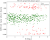 |
Fig. 1. Membership selection with CLUMPS on the PPS for the cluster M1115. The green dots represent the galaxy cluster members, while the red dots represent background and foreground galaxies. |
3.2. Spectroscopic completeness and number density profile
To compute the projected number density of the stacked cluster members N(R), we had to re-scale the projected distances of the cluster members from their corresponding cluster centre. We re-scaled each distance in units of the corresponding R200c of the cluster in order to compare member distances of different clusters and merge them to compute the N(R) profile. The evaluation of N(R) can be affected by completeness issues of the spectroscopic dataset of each individual cluster. Not accounting for spectroscopic incompleteness could lead to an erroneous estimation of the intrinsic ν(r), if the completeness function is radius-dependent. On the other hand, the velocity distribution is not affected by completeness issues, since the observational selection does not operate in redshift space within the narrow redshift range spanned by each cluster.
To determine the radial completeness of the cluster members only, we applied two colour cuts (described in detail in Appendix A) to our full photometric and spectroscopic samples in order to limit interloper contributions. The cutting process, as well as the whole spectroscopic completeness determination routine, was applied to every galaxy cluster in the sample separately. We assumed the position of the corresponding brightest cluster galaxy (BCG) as the centre of each galaxy cluster, since our sample only contains round and virialised galaxy clusters with a single BCG. We divided the region within 0 and 600 kpc into ten linearly spaced bins, while we divided the outer region from 600 to 6000 kpc into five logarithmically spaced bins. The aim of this spacing is to better sample the inner, more populated, regions of the considered galaxy clusters. For each radial bin, we computed the ratio between the number of spectroscopic objects, members and non-members, and the number of photometric objects that are within the considered bin after the two colour cuts. This ratio is the spectroscopic completeness of our sample. Hence, we assigned the corresponding completeness coefficient, namely Ci, to every cluster member according to their radial distance from the BCG.
After this, we defined another set of 100 bins linearly spanning from 0 to 6000 kpc, and for the i-th bin we computed the projected number density of members through the weighted sum of cluster members:
 (3)
(3)
where  , and Ri is the re-scaled radial boundary of the considered bin. The uncertainty ε(R), which we assigned to the N(R) profile, is that associated with Poissonian errors over counts, that is,
 (4)
(4)
To minimise its effect on the cluster dynamical state, we restricted our dynamical analysis to the virial region, which we define as the inner 1.2 R200c region, corresponding to radii of ≤R100c.
4. Colour and mass sub-sampling
The core of this work consists of studying the velocity anisotropy profile of different populations of cluster members. In this paper, we focus on four classes of galaxy cluster members: the first two are distinguished as red and blue galaxies, while the other two are classed as high mass (HM) or low mass (LM). In Table 2 we report the corresponding population subdivision, while in the next sub-sections we explain in detail how we assigned every cluster member in each category.
Number of spectroscopically confirmed cluster members for each galaxy cluster.
4.1. Colour subdivision
We selected the red and blue members through a recursive linear fit of each cluster’s red sequence in the R-band magnitude versus B−R colour plot. In the i + 1-th iteration of the linear fit, we excluded cluster members that fall outside the 2 or 1σ region (depending on the cluster case) around the best fit of the i-th iteration. The algorithm stops when the mi + 1 angular coefficient of the linear best fit satisfies (mi + 1 − mi)/mi < 0.03. In Fig. 2, we show an example of colour subdivision for M0329, in which the red dots mark the cluster members belonging to the red sequence. Member galaxies in the so-found red sequence are classified as ‘red’, while the others are labelled ‘blue’.
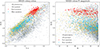 |
Fig. 2. Colour subdivision for the members of M0329, both on the colour-colour plane (V−I versus B−R; left panel) and on the R-band magnitude versus B−R colour plane (right panel). The latter is the plot used to determine which galaxies are red and which are not, according to the recursive red sequence linear fit. The “all-matched” entry in the legend, corresponding to the yellow points, represents the objects in the photometric catalogue that have a match in the spectroscopic catalogue. |
4.2. Mass subdivision
The second subdivision we opted for is related to the stellar mass, M*, of the selected cluster members. We divided our sample in two classes of galaxies: HM and LM members. For the purposes of this simple subdivision, we adopted the I-band magnitude of cluster members as a stellar mass proxy (see e.g. Pozzetti et al. 2007; Mercurio et al. 2021) as it allowed an easy identification of the two categories. We separated the two components by identifying a dip in the I-band magnitude distribution of each cluster, at magnitude Idip, as it represents the crossing point of two different galactic mass functions (Annunziatella et al. 2016; Mercurio et al. 2021). Hence, we define cluster members with I < Idip as HM and those with I > Idip as LM.
5. Methods of the dynamical analysis
Following a common practice in the existing literature, we stacked the cluster members of our sample in a normalized PPS, under the hypothesis of homology between galaxy clusters (Navarro et al. 1996, 1997, 2004). We normalized the cluster-centric distance of each member galaxy with respect to the original cluster R200c value and their rest-frame line-of-sight (LOS) velocity with respect to the quantity
 (5)
(5)
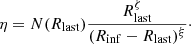
We then re-scaled the normalized cluster-centric radii and rest-frame LOS velocities by the mean values of R200c and v200, respectively, to emulate a real cluster. The newly formed stacked cluster is composed of 4176 cluster members, which belong to different populations; in Fig. 3, we present how different galaxy populations were distributed within the re-scaled PPS.
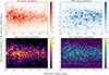 |
Fig. 3. PPS of major cluster-member populations of this work, re-scaled by the mean value of R200c and v200. The scale at the right of every plot represents the number of objects in each bin. We note that the blue galaxies, as expected, are more concentrated towards the outer regions of our ensemble cluster, while the red ones are mostly found in the inner regions. The HM population, despite it being radially distributed almost the same as the LM population, is slightly less spread out in terms of velocity than the latter. |
In this work we implemented two different strategies to measure the velocity anisotropy profile, β(r), in the stacked galaxy cluster. The first approach to the dynamical problem is through a parametric description of the β(r) profile, which was realized via the MAMPOSSt (Mamon et al. 2013) method using the MG-MAMPOSSt (Pizzuti et al. 2021, 2023) code; the second approach is through the inversion of the JE (see e.g. Binney & Mamon 1982; Solanes & Salvador-Sole 1990; Dejonghe & Merritt 1992 or Appendices A and B in Mamon et al. 2019 for equivalences between different inversion methods), with the aim of computing β(r) in a non-parametric way. Employing two different methods also allowed us to cross-check the results that we show in Sect. 6.
5.1. Parametric analysis with MAMPOSSt
As mentioned in the introduction, MAMPOSSt adopts parametric profiles for ν(r), M(r), and β(r). Throughout this paper, we explore different combinations of the following models.
For the number density, ν(r), we tested two well-known models:
-
the NFW profile (Navarro et al. 1997), given by
 (6)
(6) -
the Hernquist profile (Hernquist 1990), given by
 (7)
(7)
We directly fitted the projected number density profile, N(R), with both the NFW and the Hernquist profiles, through a maximum likelihood Bayesian algorithm (see Maraboli et al. 2025), and we give the resulting parameter values as an input to MG-MAMPOSSt. In Fig. B.1, we show the projected number density profiles, N(R), for the different galaxy populations studied in this work, and the corresponding NFW (and Hernquist) profile fits.
For the total mass profile, M(r), we employed the NFW model again, that is,
![Mathematical equation: $$ \begin{aligned} M_{\rm NFW}(r) = 4\pi \rho _{\rm NFW}r_{\rm NFW}^3\left[\ln {\left(1+\frac{r}{r_{\rm NFW}}\right)}-\frac{r}{r+r_{\rm NFW}}\right], \end{aligned} $$](/articles/aa/full_html/2026/04/aa57879-25/aa57879-25-eq10.gif) (8)
(8)
and the Hernquist model,
 (9)
(9)
Finally, for the velocity anisotropy profile, β(r), we tested two models from a general class of models, written as
 (10)
(10)
Here, we have four free parameters: β0 = β(r = 0), β∞ = limr → +∞β(r), rβ is a scale radius, and δ is a fixed exponent. In this work, we tested the specific cases in which δ = 1, that is, with the known generalised Tiret (gT) model (Tiret et al. 2007); and in which δ = 2, with the generalised Osipkov–Merritt (gOM) model (Osipkov 1979; Merritt 1985). For these models, MAMPOSSt assumes that rβ = r−2 = rNFW = rH/2, where r−2 is the radius at which dlnρ/dlnr = −2 and ρ(r) is the total mass density profile. We remark that in our analysis we took into consideration all the possible combinations of the ν(r), M(r), and β(r) profiles.
5.2. Numeric Jeans inversion
The second method that we employed is the so-called JI, which is an almost fully non-parametric solution of the JE that allows users to extract the β(r) profile (Binney & Mamon 1982; Solanes & Salvador-Sole 1990; Dejonghe & Merritt 1992). This technique does not need to fit the stacked cluster’s N(R) or its σlos(R) profiles, which we just smoothed with the LOWESS method (see e.g. Gebhardt et al. 1994), and it only needs the total mass profile as an input.
Our code for the JI solves the JE in the formulation Solanes & Salvador-Sole (1990) and Dejonghe & Merritt (1992), which splits the problem in a set of simpler equations. Since these equations contain integrals up to infinity, we had to extrapolate N(R) and σlos(R) to a sufficiently large radius that can mimic infinity. We chose to set this ‘infinity radius’ Rinf at 30 Mpc from the stacked cluster centre, and in Sect. 7 we thoroughly discuss how the choice of this and other arbitrary parameters affects the results of the JI.
5.2.1. Extrapolation of N(R) and σlos(R)
The extrapolation process follows that described in Biviano et al. (2013), in which the N(R) and the σlos(R) profiles were treated separately. Beyond the last observed radius, Rlast, the extrapolation was done according to Eq. (10) in Biviano et al. (2013) for N(R); for completeness, we report it here:
 (11)
(11)
where
 (12)
(12)
and
 (13)
(13)
We note that the only free parameter in this formulation is ξ. For our analysis, we set ξ = 0.5 based on our experience, and we discuss the impact of this (and of Rinf) choice on the results in Sect. 7. The extrapolation method of σlos(R) instead assumes that σlos(Rinf) = fσmax, where σmax is the σlos(R) peak value and f a fixed as constant, and it is a log-linear interpolation:
 (14)
(14)
where σlast = σlos(Rlast). We set the value of f to 0.2, since with this value we observe that σlos(Rinf) assumes values comparable to the velocity dispersion of field galaxies. Once N(R) and σlos have been extrapolated, they can be employed in the JI equations of Solanes & Salvador-Sole (1990) and Dejonghe & Merritt (1992).
5.2.2. Ensemble mass profile
The last input required to obtain the β(r) anisotropy profile from the JI equations is the total mass profile of the stacked cluster. Following a common method in the literature (Biviano & Katgert 2004; Katgert et al. 2004; Biviano & Poggianti 2009; Mamon et al. 2019), we built a mass profile that mimics the average properties of the real galaxy clusters in our sample. We based this process on three fundamental considerations:
-
(a)
The projected numerical density N(R) of the stacked cluster is the mean of each cluster N(R), naturally weighted by their respective numbers of cluster members.
-
(b)
The average of more analytic mass profiles, such as NFW or Hernquist, is not an analytic mass profile, whereas an analytic mass profile with average parameter values is.
-
(c)
The physical scales of a cluster, such as its R200c or M200c, are the most important ones to reproduce through the averaging process.
The first key point led us to perform every average using the number of cluster members as weights. Hence, within this section the mentioned averages are always weighted on the number of members of the respective galaxy cluster and written as ⟨ ⋅ ⟩. The second key point led us to compute the total mass profile via averaged parameters instead of averaging different total mass profiles. In doing so, we were able to link the behaviour of the velocity anisotropy profiles that we show in Sect. 6 to a well-identified total mass profile. The last key point is directly linked to the computation of the total mass profile, where we refer to Eq. (11) in Mamon et al. (2019) and its reformulation in terms of virial quantities:
 (15)
(15)
where
 (16)
(16)
are the expressions for the NFW and Hernquist model, respectively. Hence, there are two quantities needed to compute these profiles are two to be chosen from R200c, c200c, and r−2 = R200c/c200c. From Umetsu et al. (2018), we obtained the corresponding R200c, c200c, and r−2 ≡ rNFW for every galaxy cluster in our sample. We set the value ⟨R200c⟩ = 2.13 ± 0.20 Mpc as R200c of the ensemble cluster; from this, the corresponding M200c value of (1.51 ± 0.41)×1015 M⊙ (assuming ⟨z⟩ = 0.315 as the redshift of the stacked cluster) follows. Since ⟨r−2⟩≠⟨R200c⟩/⟨c200c⟩ and so on with the other relations among R200c, c200c, and r−2, following key point (c) we defined the average concentration of the ‘synthetic’ mass profile as
 (17)
(17)
We remark that the data from Umetsu et al. (2018) concerning M200c and c200c were obtained through a NFW fit of the cosmic shear measurements, and it is worth checking their robustness when transposed to a Hernquist model. Naturally, in our sample of round and virialised galaxy clusters, each of them should have a single value of r−2 of their mass density distribution, which can be consequently identified as r−2 ≡ rNFW ≡ rH/2. However, the r−2 predicted from the NFW fit can be shifted by some systematics in the analysis with respect to a hypothetical Hernquist fit of the cosmic shear measurements. Hence, we tested the ‘single r−2 hypothesis’ by exploiting the results of Maraboli et al. (2025), in which the authors fitted the total mass profile of each cluster in their sample with different mass models, including NFW and Hernquist. We find that for all the clusters in Maraboli et al. (2025), the relative discrepancy between  and
and  is
is  . Then, from Umetsu et al. (2018) we were able to directly obtain
  for each galaxy cluster in our sample, compute
  , and repeat the process for
  , where the
  of each cluster is computed as
  . With this recipe for the total mass profiles (as we did in the MAMPOSSt analysis) we also used the JI to study two different cases: the NFW and the Hernquist profile. For these two models, we computed the following scale values according to our method: rNFW = 0.81 ± 0.44 Mpc,
  , rH = 1.43 ± 0.8 Mpc, and
  .
.
6. Results
Throughout our analysis, we tested a great number of different combinations of models (for mass, projected number density, and velocity anisotropy profiles) and galaxy populations. In the whole MAMPOSSt analysis, we explored all the possible configurations among two total mass models (NFW and Hernquist), two N(R) models (again, NFW and Hernquist), two β(r) models (gT and gOM), three colour population choices (red and blue populations and a combination), and three mass population choices (HM or LM populations and both together), for a total of 72 combinations. On the other hand, in the JI analysis the inputs are just the two choices of the total mass profile, the three colour population choices, and the three mass population choices, for a total of 18 combinations.
The confidence intervals that we report for the MAMPOSSt analysis are defined as follows: we extracted 500 samples of parameters from the Markov chains produced by MG-MAMPOSSt, which generated 500 new β(r) profiles; then, at any radius, r0, we took the 16th and the 84th percentiles of the β(r0) value distribution, and we considered them as the boundaries of our confidence levels. The best-fit profile is the one generated by the median value of the fitted parameters. For the confidence intervals of the JI, we followed a method similar to the previous one, which we explain in full detail in Sect. 7.4.1. The best JI profile was computed as described in Sect. 5.2, with all the parameter values that we list there.
In Fig. 4, we show both the MAMPOSSt and the JI results for the whole population of cluster members. We added to this comparison a new anisotropy profile, indicated as BP (Pizzuti et al. 2025b), discussed in detail in Sect. 7.2.
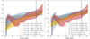 |
Fig. 4. Comparison between β(r) profiles from the two methods of the whole cluster member population. In the left panel, we plot all the MAMPOSSt outcomes with an NFW total mass profile, as well as both the JI results (NFW and Hernquist) for reference. In the right panel, similarly, we plot all the MAMPOSSt outcomes with a Hernquist total mass profile. The vertical black line represents the R200c of the stacked cluster. |
6.1. MAMPOSSt results
The β(r) and β′(r) profiles obtained from the MAMPOSSt analysis, shown in Figs. B.2 and B.3, outline two major features:
-
The choice of total mass and projected number density model can impact the resulting velocity anisotropy profiles.
-
In the vast majority of model configurations, there are no significant changes in the β(r) and β′(r) shapes for the different cluster members.
We plot all the MG-MAMPOSSt configuration results in Appendix B. Moreover, we report the median values of β0 and β∞ for each configuration of mass, number density, anisotropy model, and galaxy population in Tables B.1 and B.2.
It is easy to verify that the anisotropy profiles computed with a gT model (Fig. B.3) are strongly consistent with the corresponding anisotropy profiles computed with a gOM model (Fig. B.2; see also Fig. 4), as is naturally expected. Moreover, in every configuration there is a monotonic growth of the velocity anisotropy values with the cluster-centric distance, outlining a predominance of radial orbits in the outskirts of the cluster and more isotropic orbits towards the centre.
6.1.1. Major populations
The behaviour of the major cluster member populations (red, blue, HM, and LM galaxies, and all of them together) is, at most radii, not depending on the population itself, and all their corresponding anisotropy profiles result to be consistent with each other. We find that the anisotropy values are most sensitive to the choice of the projected number density model, and they were, in general, higher when we adopted the NFW model and lower with the Hernquist model. Among all galaxy populations, the red one is the least sensitive to N(R) changes, while the LM one is the most influenced. The general sample is also sensitive to N(R) changes.
We note a more marked discrepancy between red and blue galaxies at large radii. Nevertheless, the entity of such discrepancies is highly dependent on the chosen models for M(r), N(R), and β(r). Overall, we can conclude that the major galaxy populations follow almost the same anisotropy profile, although there are hints of a possible differentiation between red and blue cluster members.
6.1.2. Minor populations
The β(r) profiles of minor cluster member populations (red with high M*, red with low M*, blue with high M*, blue with low M*) do not exhibit significant differences in terms of anisotropy values, and we were able to reach almost the same conclusions obtained for the major populations. Due to the smaller number of objects in each class, the results for the minor populations are naturally more sensitive to the model choice, and they have larger confidence intervals; this limited our possibilities for observing significant differences among them.
6.2. Jeans inversion results
As for the MAMPOSSt results, in Fig. C.1 we show the velocity anisotropy radial profiles resulting from the JI for both of the considered total mass profiles. This technique allows a sharper inspection of the velocity anisotropy profile, due to its un-parametrised formulation, overcoming the rigidity of a fixed functional form as those implemented in the MG-MAMPOSSt code.
The general trend followed by the resulting β(r) is similar to that outlined by the MG-MAMPOSSt analysis; we again find more isotropic orbits towards the centre of the cluster, and more radial orbits towards the outskirts of the ensemble cluster. In addition to this, the JI results present a very interesting feature at intermediate radii. In every studied population (as well as in the whole sample of cluster members), we observe a local maximum in β(r) at ∼250 kpc from the cluster centre and a consequent local minimum at ∼r−2, while after that point β(r) starts increasing again, returning to the original growing trend. As we find in the MAMPOSSt analysis, there are no significative changes between the velocity anisotropy profiles of different cluster member populations, since the 1σ confidence intervals of the presented β(r) are often overlapping. However, in concordance with what we show in the previous sub-section for MAMPOSSt, these β(r) profiles might suggest that red galaxies have more radial orbits in the outskirts. In any case, according to the JI analysis these differences are too small to be conclusive, and we can state that the orbital anisotropy of cluster members does not depend on the chosen galaxy population.
The two tested total mass profiles do not produce significantly different β(r) results. Nevertheless, this fact matches our expectations: since the choice of the mass model is just a way to represent the same true total mass profile of a cluster, the outcomes of the two models are not very different.
7. Discussion
So far, several studies have investigated the velocity anisotropy profiles of different cluster member populations, both from the observational and simulation points of view. Starting from the simulation side, much effort has been put in the analysis of the general anisotropy properties of dark-matter halos (Wojtak et al. 2005; Hansen & Moore 2006; Ascasibar & Gottlöber 2008; Lemze et al. 2012), while, only recently there has been a focus on more specific cluster member populations (Lotz et al. 2019; He et al. 2024; Abdullah et al. 2025). The results of these cosmological N-body simulations consistently agree on what the typical β(r) values in galaxy clusters should be: a growing profile with central values of β0 ≳ 0 and β(R200)≈0.5 − 0.7. As we show in Sect. 6, the anisotropy profiles that we find in the MAMPOSSt analysis provide an excellent confirmation of the simulation results; the JI results, except for the central peak at R ∼ 0.25 Mpc, confirm this trend as well. The general growth of the anisotropy values can be observed in almost any configuration that we considered (Figs. B.2, B.3, B.4, and B.5), and the values that we find are also very similar to the corresponding mock populations (see for reference, Figs. 11 and 13 in Lemze et al. 2012 or the upper right panels of Fig. 3 in Lotz et al. 2019).
On the other hand, the observed anisotropy profiles present a wider phenomenology, probably due to the variety of sample characteristics explored in the literature. Biviano & Katgert (2004) studied the ESO Nearby Abell Cluster Survey (ENACS; Katgert et al. 1996) sample by subdividing the cluster members into morphological categories. They determined the total mass profile, using elliptical and S0 kinematics, under the assumption of isotropic orbits, which was supported by the analysis of the shape of their velocity distribution (Katgert et al. 2004). They found that spirals move on radial orbits (see Figs. 6 and 8 therein). It is interesting to compare their spiral galaxy results with our blue sample and its subdivisions into HM and LM blue galaxies; we can see that, although we find anisotropy values slightly higher than theirs for these populations, our blue sample (especially the LM part, which is the majority) is generally more isotropic than the other populations. This is at variance with what was suggested by Biviano & Katgert (2004). We think that this difference could be ascribed to the different categorisation of cluster member populations, based on morphology rather than on colour. Another possibility is that the isotropic assumption of Biviano & Katgert (2004) for elliptical and S0 orbits is not completely fulfilled. Another possibility is an evolution with redshift of the anisotropy profiles, since our clusters are located at higher z than those of Biviano & Katgert (2004). However, a more recent study by Mamon et al. (2019) did not find a significant difference in the orbits of cluster galaxies of different morphologies at lower redshifts, using the spectroscopic dataset of the clusters of the Wide-field Nearby Galaxy-clusters Survey (WINGS; Cava et al. 2009; Moretti et al. 2014) that is limited to 0.04 < z < 0.07. In this low-z sample, β(r) also shows the same growing trend with r for all considered cluster galaxy populations.
An argument in favour of the redshift dependence of the anisotropy profile was presented by Biviano & Poggianti (2009, see Fig. 4 therein), in which the high-z sample is more similar to ours since the considered clusters have 0.393 < z < 0.794 (albeit the considered cluster mass values, M200c, are in the 0.7 − 13.6 × 10¹⁴ M⊙ range, with a mean (median) value of 2.8 (4.4)×1014 M⊙). They divided their cluster member sample into two galaxy populations (by the presence or absence of emission lines in their spectra), and they did not find significant differences between the corresponding anisotropy profiles. Our extensive work confirms this result, providing much stronger evidence of the common shape of β(r) regardless of the galaxy population.
Two other very recent works (Valk & Rembold 2025; Pizzuti et al. 2025a) investigated the orbital behaviour of different cluster member populations, adopting the same techniques as ours. Valk & Rembold (2025) studied a stack of 642 low-redshift (z ≲ 0.2) galaxy clusters from the Sloan Digital Sky Survey (SDSS; York et al. 2000), both with MAMPOSSt and JI, which were divided into relaxed and non-relaxed clusters according to a Gaussianity criterion applied to the observed LOS velocity probability distribution. The relaxed sample, which has an overall β(r) profile strongly consistent with other low-z samples such as Biviano & Poggianti (2009) and Mamon et al. (2019, see the upper panel of Fig. 4 therein), was further divided into four populations: active galactic nuclei and star-forming, transition, and quiescent objects. All four populations show very similar anisotropy values (Fig. 6), confirming the growing trends and corroborating the evidence of a ‘universal’ anisotropy profile. Pizzuti et al. (2025a) analysed a stack of 75 clusters from the CHEX-MATE sample (CHEX-MATE Collaboration 2021), spanning a wide redshift range up to z = 0.55, with MG-MAMPOSSt. They found a possible hint of a correlation between cluster mass and anisotropy profile.
To sum up, from the comparison of our results to other relevant works in this field, we conclude that there is no significant evidence of a different β(r) for different cluster galaxy populations in the explored redshift ranges. In the companion work by Biviano et al. (2026, which is based on the same sample used here), we find evidence of β(r) evolution of the total cluster member population by comparing the Biviano et al. (2026) anisotropy profiles with those of galaxy clusters at z ≃ 0 (Mamon et al. 2019; Valk & Rembold 2025). Specifically, orbits appear to become more isotropic with time. Instead, it is more difficult to conclude if different galaxy populations evolved their orbits together or at separate times. While Biviano & Poggianti (2009) suggested β(r) evolution for the quiescent population and not for the star-forming one, their result is not statistically significant. As a matter of fact, both in our sample and in the higher z sample of Biviano et al. (2021), the red and quiescent populations have β(r) values slightly higher than those of the blue and star-forming populations, at least outside the cluster centre. However, in the low-z sample of Mamon et al. (2019), the early-type galaxies display a lower β(r) with respect to the late-type galaxies. Comparing these results is not straightforward, because of the different characterisation of the different cluster galaxy populations based on colour, morphology, or star-formation activity, and because the different samples have different stellar mass limits.
7.1. Orbital evolution and cluster history
The general framework that is suggested by the comparison between our work and the existing literature may lead to a comprehensive interpretation of a galaxy cluster history based on its orbital behaviour throughout time. Numerical simulations (see e.g. Lemze et al. 2012; Abdullah et al. 2025) show that the orbital behaviour of cluster members, i.e. β(r), depends on the mass of the considered cluster, as well as on its redshift and relaxation status. Particularly, the higher the cluster mass or redshift, the higher its anisotropy values.
The anisotropy-relaxation relation is more complex and may depend on the phase of the relaxation process. Collisions and major mergers disrupt the phase-space distribution of cluster members, causing violent relaxation (Lynden-Bell 1967), which erases ordered motions and causes isotropisation of the orbits (Lemze et al. 2012). After a dynamical time, the cluster relaxes and proceeds with a smooth accretion process of field galaxies from surrounding filaments, on radially elongated orbits, so radial anisotropy develops again but mostly in the external cluster regions (Lapi & Cavaliere 2011). Therefore, it is not trivial to determine the interplay between these processes and which prevails on the others. However, the measurements made in the last ∼20 years of different (in terms of mass, redshift, and relaxation status) galaxy cluster samples can help to draw a picture of the cluster’s dynamical history and evolution. At high redshifts, right after the birth of a cluster, its total mass is low, the virialisation has not been completed yet, and the orbits are almost isotropic (Biviano et al. 2016, 2021). At intermediate redshifts, as we observe in this work, the virialisation process has been fully completed2, and a galaxy cluster had enough time to accrete and raise its total mass through cosmic filaments. The newly accreted cluster members are naturally moving along very radial orbits, and this fact makes anisotropy values rise at all radii. At very low redshifts, there has been enough time to allow the majority of the observed clusters to undergo multiple collisions or major mergers, which can bring them back to a more isotropic state, as observed, for example, by Mamon et al. (2019) and by Mitra et al. (2024).
7.2. Method comparison
The two methods presented here offer different approaches to the same problem: the MG-MAMPOSSt code performs Monte Carlo Markov chain (MCMC) fitting of parametric β(r) profiles, inspired by the suggestions coming from cosmological simulations (see e.g. He et al. 2024), while the non-parametric formulation of the JI allows for a more flexible characterisation of the orbital anisotropy. The MAMPOSSt and JI results are in agreement for most of the considered projected radii, depending on the choice of the models used in MAMPOSSt, which, in some cases, can create localised discrepancies at some radii (see Figs. B.2, B.3, and C.1). For convenience, in Fig. 4 we overlap the gT, gOM, and JI results for the global population as an example. From this plot, we can clearly see that the two methods are in total agreement when characterising the anisotropy profile at large radii, denoting highly radial orbits (β′(r)≈2) in that region. On the other hand, in the innermost regions both methods highlight that orbits are closer to isotropy than in any other region of the cluster. However, between 0.5 and 1.5 Mpc, we find some differences for the two methods: although the confidence intervals of the profiles are still slightly overlapping, the monotonic trend observed in the MAMPOSSt profile is not followed by the JI one. The shape of the JI β(r) has the peculiarity of a sudden change of direction after a very steep increment of the anisotropy values in the first ∼250 kpc, followed by an intermediate region of more isotropic orbits that is later reconnected to the outer region with higher anisotropy values. The built-in MG-MAMPOSStβ(r) profiles are too “rigid” to capture such a feature, and they can only catch the general trend of it. Since the NFW and the Hernquist profiles are robustly verified to be good one-component total-mass models for clusters of galaxies (e.g. Appendix C in Bonamigo et al. 2018; Maraboli et al. 2025), they are also a suitable input for the JI process. This fact could indicate the JI as a more accurate probe for the velocity anisotropy profile, especially in this analysis of a very rich ensemble cluster. To further check if this discrepancy comes from the rigidity of the MG-MAMPOSStβ(r) models of Eq. (1), we implemented and tested a new ansatz for the anisotropy, which is designed to account for the bump found in the JI results (Pizzuti-Biviano, hereafter BP; Pizzuti et al. 2025b):
![Mathematical equation: $$ \begin{aligned} \beta _{\rm BP}(r)=\beta _0+(\beta _\infty - \beta _0)\left[\frac{r}{r+r_\beta }+\frac{r^2}{r^2_\beta } e^{-\left(\frac{r}{r_\beta }\right)^2}\right], \end{aligned} $$](/articles/aa/full_html/2026/04/aa57879-25/aa57879-25-eq30.gif) (18)
(18)
where rβ defines the position of the bump. We considered rβ as a free parameter in the MG-MAMPOSSt fit. We show the results in Fig. 4 for the total population. We checked for the significance of the JI feature by comparing the MG-MAMPOSSt BP and gT model results with the Bayesian information criterion (BIC; Schwarz 1978). With both the NFW and the Hernquist total mass profiles, we find ΔBIC = BICBP − BICgT ∼ 6, indicating that the gT model is strongly favoured compared to the BP model (Kass & Rafferty 1995), which made us question the physical reality of the β(r) feature found in the JI analysis. Moreover, we carefully investigated the possible origin of the JI feature with additional tests: (1) we re-scaled with r−2 instead of R200c, but this parametrisation resulted to be weaker since r−2 is more poorly constrained than R200c from the Umetsu et al. (2018) data (mostly because of the large errors on the values of concentration); (2) we tested if one of the clusters composing the stack was ‘problematic’, and we re-ran the JI analysis, removing one cluster at a time from the stack; (3) we tested if the JI feature was an artefact of the interpolation to R = 0 made by the JI analysis software by recomputing the velocity dispersion profile at smaller radii to limit the interpolated radial range. However, none of these tests succeeded in removing the JI β(r) feature. We conclude that while the data, taken at face value, indicate the existence of the β(r) feature, the statistics provided by our dataset does not allow for a robust confirmation of it.
7.3. General interpretation
The behaviour of the velocity anisotropy profiles that we find with both the adopted techniques can be traced back to some known physical processes that involve galaxy clusters. Starting from the outer regions of the ensemble cluster, the highly radial orbits that we find in that area can be traced to the new infalling galaxies that recently joined the cluster. This consideration explains why the velocity anisotropy values at those radii are higher than in any other region of the cluster. When a galaxy falls from the surrounding environment towards the cluster centre, its orbit is mostly radial; instead, when we consider regions that are below the virial radius, cluster members begin to be more and more isotropic.
In the innermost regions of the cluster –below ∼250 kpc– we find velocity anisotropy values that are lower than the others. This time, we reconnected this specific behaviour to the presence of dynamical friction (Chandrasekhar 1943), because at these radii the cluster environment is very crowded (as we can see from Fig. B.1). Since the dynamical friction force is directly proportional to the velocity of the object experiencing it, the principal component of the orbital velocity will be affected the most by friction, whether it is the tangential or the radial component. Hence, this process results in the orbital velocity components being roughly equal, and so it leads to isotropy.
At intermediate radii, where the two methods produce different results for β(r), the MAMPOSSt outcomes naturally return a smooth transition between the radial orbits of the cluster outskirts and the more isotropic ones at the centre. The JI results, instead, offer a more intriguing view on the dynamics of cluster members at intermediate radii, between 250 and 1500 kpc.
7.4. Insight into the methodologies
The techniques that we adopted to study the velocity anisotropy profiles have been thoroughly tested and have been proven to be robust estimators of the β(r) profiles (e.g. Biviano & Katgert 2004; Biviano et al. 2013, 2024; Annunziatella et al. 2016; Mamon et al. 2019; Sartoris et al. 2020; Biviano et al. 2026). As every method, there are some aspects that we believe are worth examining to better comprehend the results that we present in Sect. 6. Further discussion about the JI technique can be found in Appendix C.
First, we want to address how the adoption of the mass profiles described in Sect. 5.2.2 affected our MAMPOSSt analysis, since the scale radii (and their confidence intervals) determined in that section are directly involved in the priors given to MG-MAMPOSSt. The code, as we report in Sect. 5.1, fixes the scale radius of the selected beta model, rβ, to the r−2 of the total mass profile. We set the prior for the total mass scale radius, rs, as a uniform distribution between  and
and  , where
  is set as the value of rNFW or rH (depending on the chosen configuration) computed in Sect. 5.2.2, and σr is its corresponding error.
7.4.1. Jeans inversion error contributions
Another interesting topic relating to the total mass profile for the stacked cluster is how this choice impacts the systematic errors of our results. The confidence intervals that we report in Fig. C.1 are indeed the final product of many factors of uncertainty. We identify and characterise two main sources of it below.
-
First is the set of arbitrarily chosen parameters that were to be made in order to compute the β(r) profile, as they represent the most relevant component of the systematic errors in our analysis. This set includes the smoothing factors for N(R) and σlos(R); the constants ξ and f employed in Eqs. (11) and (14), respectively; the infinity radius, Rinf; and the scale radii of the total mass profiles, rNFW and rH.
-
Second is the statistical errors that naturally come from our data, namely from the velocity dispersion radial profile, σlos(R), and the projected number density profile, N(R).
Although the uncertainties related to the total mass profiles that we adopted for the JI are related to those in Umetsu et al. (2018), we included them among the systematics because of the profile-building process that we describe in Sect. 5.2.2. The resulting total mass profile was determined based on a set of reasonable, but arbitrary, choices about its fundamental quantities, such as the definition of the ensemble cluster concentration  (Eq. 17) and the definition of its r−2.
In Fig. C.2 we report, as an example, the velocity anisotropy profile for the whole sample of blue cluster members, with the confidence intervals dissected according to the characterisation explained above. From this plot, it is clear that the bootstrap of the N(R) and σlos(R) profiles is the main source of uncertainty, while the systematic one is marginal. We also notice some correlation between the two kinds of errors, since the general confidence interval width does not correspond to the sum of the two interval widths.
7.4.2. Variance of the cluster sample
Our cluster sample offers the rare opportunity to analyse it both through the stacking of its components, as we did in this work, and in the cluster-by-cluster way described by Biviano et al. (2026). In the latter a significant variance in β(r) emerged among the considered clusters; however, their average β(r) is in good agreement with the average β(r) from the GAEA-simulated halos of similar mass and redshift, which is also consistent with our results. Biviano et al. (2026) suggested that this variance could be due to the different cluster orientations relative to their major axis, and we refer to Sect. 5 of that work for an extended discussion on the variance origins.
8. Summary and conclusions
In this work, we compared two robust techniques for measuring the orbital velocity anisotropy profile, β(r), in a stack of galaxy clusters, namely the MAMPOSSt method and the JI. Thanks to our very large number of cluster members, from these two parallel analyses we were able to obtain a clear, general picture of how the β(r) profiles behave for different cluster member populations. We summarise our work herein the points listed below.
-
We considered a sample of nine massive galaxy clusters at intermediate redshifts (M200c > 7 × 10¹⁴ M⊙, 0.18 < z < 0.45; see Table 1), selected from the CLASH-VLT (Rosati et al. 2014) targeted clusters. Our main goal was to study the behaviour of the velocity anisotropy profile, β(r), for different galaxy populations, and we did so by stacking the cluster members in a re-normalised PPS and considering them as a part of a single ensemble cluster.
-
The selection of cluster members was based on a re-calibrated version of the CLUMPS algorithm, which operates on the galaxy distribution in the PPS and looks for local minima of the surface number density of spectroscopic objects (see Fig. 1). The selected members were then labelled as red or blue galaxies depending on their belonging to the red sequence (Sect. 4.1). They are also labelled as high or low stellar mass galaxies according to their I-band magnitude (Sect. 4.2).
-
We stacked the member galaxies of different clusters in the same PPS by normalising their distance from the cluster centre by the corresponding cluster, R200c, and their rest-frame velocity by
 . Then, we re-scaled the galaxy PPS coordinates by ⟨R200c⟩ = 2.18 Mpc (⟨ ⋅ ⟩ denotes “average weighted” with respect to the number of cluster members) and ⟨v200c⟩ = 1732 km/s, respectively.
 -
After the stacking procedure, we produced the surface number density profiles, N(R) (Fig. B.1), for the different cluster member populations. This required properly accounting for the spectroscopic completeness of our sample (Sect. 3.2), which was consequently employed to weight the contribution of each cluster member to N(R).
-
Finally, we analysed the cluster members via two different methods: the MAMPOSSt method (Sect. 5.1), which performs a MCMC fit of the PPS adopting the parametric profiles for N(R), M(r), and β(r) presented in Eqs. (6), (7), (8), (9), and (10); and the JI (Sect. 5.2), which returns a non-parametric measure of β(r) upon providing the total mass profile from Eqs. (8) and (9) as input.
The results of these two parallel analyses outline a growth of the anisotropy values from the centre to the outskirts for every considered cluster member population, with β′=σr/σϑ values of ≲1.4 at the very centre and of ≳2 at the virial radius. These values can vary depending on the models and methods adopted, but the general trend is always confirmed. We find a possibly interesting feature in all the β profiles from the JI technique; that is (see Fig. C.1), the sudden switch at 250 − 400 kpc from rapidly increasing anisotropy values to a mild, but evident, decrement in the following 500 − 700 kpc, which finishes with a final increase that matches the high anisotropy values found in the MAMPOSSt analysis.
We do not find significant differences in β(r) among the studied galaxy populations, although some differences are suggested for certain choices of M(r), N(R), and β(r) between the red and blue populations at large radii. As we discuss in Sect. 7, this behaviour is consistently maintained throughout the evolution of a galaxy cluster, which may change the overall orbital anisotropy of its components.
The very high precision of our results, based on an unprecedented number of cluster member redshifts, and the robustness of our techniques make the obtained β(r) profiles a reliable measurement of velocity anisotropy in clusters of galaxies. The mathematical simplicity of the anisotropy profiles found with the MAMPOSSt method makes them a suitable and ready-to-use tool for future dynamical mass measurements. On the other hand, the freedom allowed by the JI in determining the true shape of the velocity anisotropy profile sheds light on new potentially interesting dynamical features of galaxy clusters. Measuring such features could improve our current knowledge of galaxy cluster structure and, consequently, provide new inputs for diverse cosmological studies that rely on them.
References
- Abdullah, M. H., Mabrouk, R. H., Ishiyama, T., et al. 2025, ApJ, 987, 70 [Google Scholar]
- Aguirre Tagliaferro, T., Biviano, A., De Lucia, G., Munari, E., & Garcia Lambas, D. 2021, A&A, 652, A90 [NASA ADS] [CrossRef] [EDP Sciences] [Google Scholar]
- Annunziatella, M., Mercurio, A., Biviano, A., et al. 2016, A&A, 585, A160 [NASA ADS] [CrossRef] [EDP Sciences] [Google Scholar]
- Ascasibar, Y., & Gottlöber, S. 2008, MNRAS, 386, 2022 [CrossRef] [Google Scholar]
- Bacon, R., Accardo, M., Adjali, L., et al. 2010, SPIE Conf. Ser., 7735, 773508 [Google Scholar]
- Bertin, E. 2011, ASP Conf. Ser., 442, 435 [Google Scholar]
- Bertin, E., & Arnouts, S. 1996, A&AS, 117, 393 [NASA ADS] [CrossRef] [EDP Sciences] [Google Scholar]
- Bezanson, R., Labbe, I., Whitaker, K. E., et al. 2024, ApJ, 974, 92 [NASA ADS] [CrossRef] [Google Scholar]
- Binney, J., & Mamon, G. A. 1982, MNRAS, 200, 361 [Google Scholar]
- Binney, J., & Tremaine, S. 1987, Galactic Dynamics (Princeton: Princeton University Press) [Google Scholar]
- Biviano, A., & Katgert, P. 2004, A&A, 424, 779 [NASA ADS] [CrossRef] [EDP Sciences] [Google Scholar]
- Biviano, A., & Poggianti, B. M. 2009, A&A, 501, 419 [NASA ADS] [CrossRef] [EDP Sciences] [Google Scholar]
- Biviano, A., Rosati, P., Balestra, I., et al. 2013, A&A, 558, A1 [Google Scholar]
- Biviano, A., van der Burg, R. F. J., Muzzin, A., et al. 2016, A&A, 594, A51 [NASA ADS] [CrossRef] [EDP Sciences] [Google Scholar]
- Biviano, A., Moretti, A., Paccagnella, A., et al. 2017, A&A, 607, A81 [NASA ADS] [CrossRef] [EDP Sciences] [Google Scholar]
- Biviano, A., van der Burg, R. F. J., Balogh, M. L., et al. 2021, A&A, 650, A105 [NASA ADS] [CrossRef] [EDP Sciences] [Google Scholar]
- Biviano, A., Poggianti, B. M., Jaffé, Y., et al. 2024, ApJ, 965, 117 [Google Scholar]
- Biviano, A., Maraboli, E. A., Pizzuti, L., et al. 2026, A&A, 707, A153 [NASA ADS] [CrossRef] [EDP Sciences] [Google Scholar]
- Bonamigo, M., Grillo, C., Ettori, S., et al. 2018, ApJ, 864, 98 [Google Scholar]
- Butcher, H., & Oemler, A. 1978, ApJ, 226, 559 [NASA ADS] [CrossRef] [Google Scholar]
- Capasso, R., Saro, A., Mohr, J. J., et al. 2019, MNRAS, 482, 1043 [NASA ADS] [CrossRef] [Google Scholar]
- Cava, A., Bettoni, D., Poggianti, B. M., et al. 2009, A&A, 495, 707 [NASA ADS] [CrossRef] [EDP Sciences] [Google Scholar]
- Chandrasekhar, S. 1942, Principles of Stellar Dynamics (New York: Dover) [Google Scholar]
- Chandrasekhar, S. 1943, ApJ, 97, 255 [Google Scholar]
- CHEX-MATE Collaboration (Arnaud, M., et al.) 2021, A&A, 650, A104 [NASA ADS] [CrossRef] [EDP Sciences] [Google Scholar]
- De Lucia, G., & Blaizot, J. 2007, MNRAS, 375, 2 [Google Scholar]
- De Lucia, G., Fontanot, F., Xie, L., & Hirschmann, M. 2024, A&A, 687, A68 [NASA ADS] [CrossRef] [EDP Sciences] [Google Scholar]
- Dejonghe, H., & Merritt, D. 1992, ApJ, 391, 531 [NASA ADS] [CrossRef] [Google Scholar]
- Dressler, A., Oemler, A., Couch, W. J., et al. 1997, ApJ, 490, 577 [NASA ADS] [CrossRef] [Google Scholar]
- Gebhardt, K., Pryor, C., Williams, T. B., & Hesser, J. E. 1994, AJ, 107, 2067 [NASA ADS] [CrossRef] [Google Scholar]
- Gruen, D., Brimioulle, F., Seitz, S., et al. 2013, MNRAS, 432, 1455 [NASA ADS] [CrossRef] [Google Scholar]
- Hansen, S. H., & Moore, B. 2006, New Astron., 11, 333 [NASA ADS] [CrossRef] [Google Scholar]
- He, J., Wang, W., Li, Z., et al. 2024, ApJ, 976, 187 [Google Scholar]
- Hernquist, L. 1990, ApJ, 356, 359 [Google Scholar]
- Kass, R. E., & Rafferty, A. E. 1995, J. Am. Stat. Assoc., 90, 773 [Google Scholar]
- Katgert, P., Mazure, A., Perea, J., et al. 1996, A&A, 310, 8 [NASA ADS] [Google Scholar]
- Katgert, P., Biviano, A., & Mazure, A. 2004, ApJ, 600, 657 [NASA ADS] [CrossRef] [Google Scholar]
- Lapi, A., & Cavaliere, A. 2011, ApJ, 743, 127 [Google Scholar]
- Le Fèvre, O., Saisse, M., Mancini, D., et al. 2003, SPIE Conf. Ser., 4841, 1670 [Google Scholar]
- Lemze, D., Wagner, R., Rephaeli, Y., et al. 2012, ApJ, 752, 141 [NASA ADS] [CrossRef] [Google Scholar]
- Lotz, M., Remus, R.-S., Dolag, K., Biviano, A., & Burkert, A. 2019, MNRAS, 488, 5370 [NASA ADS] [CrossRef] [Google Scholar]
- Lynden-Bell, D. 1967, MNRAS, 136, 101 [Google Scholar]
- Mamon, G. A., Biviano, A., & Boué, G. 2013, MNRAS, 429, 3079 [Google Scholar]
- Mamon, G. A., Cava, A., Biviano, A., et al. 2019, A&A, 631, A131 [NASA ADS] [CrossRef] [EDP Sciences] [Google Scholar]
- Maraboli, E., Grillo, C., Bergamini, P., & Giocoli, C. 2025, A&A, 698, A272 [NASA ADS] [CrossRef] [EDP Sciences] [Google Scholar]
- Mercurio, A., Merluzzi, P., Busarello, G., et al. 2015, MNRAS, 453, 3685 [Google Scholar]
- Mercurio, A., Rosati, P., Biviano, A., et al. 2021, A&A, 656, A147 [NASA ADS] [CrossRef] [EDP Sciences] [Google Scholar]
- Merritt, D. 1985, ApJ, 289, 18 [NASA ADS] [CrossRef] [Google Scholar]
- Merritt, D. 1987, ApJ, 313, 121 [Google Scholar]
- Mitra, K., van den Bosch, F. C., & Lange, J. U. 2024, MNRAS, 533, 3647 [Google Scholar]
- Miyazaki, S., Komiyama, Y., Sekiguchi, M., et al. 2002, PASJ, 54, 833 [Google Scholar]
- Moretti, A., Poggianti, B. M., Fasano, G., et al. 2014, A&A, 564, A138 [NASA ADS] [CrossRef] [EDP Sciences] [Google Scholar]
- Navarro, J. F., Frenk, C. S., & White, S. D. M. 1996, ApJ, 462, 563 [Google Scholar]
- Navarro, J. F., Frenk, C. S., & White, S. D. M. 1997, ApJ, 490, 493 [Google Scholar]
- Navarro, J. F., Hayashi, E., Power, C., et al. 2004, MNRAS, 349, 1039 [Google Scholar]
- Osipkov, L. P. 1979, Pisma Astron. Zh., 5, 77 [Google Scholar]
- Pizzuti, L., Saltas, I. D., & Amendola, L. 2021, MNRAS, 506, 595 [NASA ADS] [CrossRef] [Google Scholar]
- Pizzuti, L., Saltas, I., Biviano, A., Mamon, G., & Amendola, L. 2023, J. Open Source Softw., 8, 4800 [Google Scholar]
- Pizzuti, L., Barrena, R., Sereno, M., et al. 2025a, A&A, 699, A88 [NASA ADS] [CrossRef] [EDP Sciences] [Google Scholar]
- Pizzuti, L., Biviano, A., Umetsu, K., et al. 2025b, JCAP, submitted [arXiv:2509.16317] [Google Scholar]
- Postman, M., Coe, D., Benítez, N., et al. 2012, ApJ, 199, 25 [Google Scholar]
- Pozzetti, L., Bolzonella, M., Lamareille, F., et al. 2007, A&A, 474, 443 [NASA ADS] [CrossRef] [EDP Sciences] [Google Scholar]
- Read, J. I., Mamon, G. A., Vasiliev, E., et al. 2021, MNRAS, 501, 978 [Google Scholar]
- Rosati, P., Balestra, I., Grillo, C., et al. 2014, The Messenger, 158, 48 [NASA ADS] [Google Scholar]
- Sartoris, B., Biviano, A., Rosati, P., et al. 2020, A&A, 637, A34 [NASA ADS] [CrossRef] [EDP Sciences] [Google Scholar]
- Schwarz, G. E. 1978, Ann. Stat., 6, 461 [CrossRef] [Google Scholar]
- Solanes, J. M., & Salvador-Sole, E. 1990, A&A, 234, 93 [Google Scholar]
- Springel, V., White, S. D. M., Jenkins, A., et al. 2005, Nature, 435, 629 [Google Scholar]
- Taylor, M. B. 2006, ASP Conf. Ser., 351, 666 [Google Scholar]
- Tiret, O., Combes, F., Angus, G. W., Famaey, B., & Zhao, H. S. 2007, A&A, 476, L1 [NASA ADS] [CrossRef] [EDP Sciences] [Google Scholar]
- Treu, T., Schmidt, K. B., Brammer, G. B., et al. 2015, ApJ, 812, 114 [Google Scholar]
- Umetsu, K., Medezinski, E., Nonino, M., et al. 2014, ApJ, 795, 163 [NASA ADS] [CrossRef] [Google Scholar]
- Umetsu, K., Sereno, M., Tam, S.-I., et al. 2018, ApJ, 860, 104 [Google Scholar]
- Valk, G. A., & Rembold, S. B. 2025, MNRAS, 536, 2730 [Google Scholar]
- Wojtak, R., & Łokas, E. L. 2010, MNRAS, 408, 2442 [NASA ADS] [CrossRef] [Google Scholar]
- Wojtak, R., Łokas, E. L., Gottlöber, S., & Mamon, G. A. 2005, MNRAS, 361, L1 [Google Scholar]
- Wojtak, R., Łokas, E. L., Mamon, G. A., et al. 2008, MNRAS, 388, 815 [Google Scholar]
- Wojtak, R., Łokas, E. L., Mamon, G. A., & Gottlöber, S. 2009, MNRAS, 399, 812 [Google Scholar]
- York, D. G., Adelman, J., Anderson, J. E., et al. 2000, AJ, 120, 1579 [Google Scholar]
M200c corresponds to the total mass within a sphere, inside which the mean mass density is 200 times the value of the critical mass density of the Universe at the redshift of the cluster.
At the mean redshift of the Biviano et al. (2021) sample,  , the look-back time is ≈8.1 Gyr, while at our mean redshift,
  , the look-back time is ≈3.6 Gyr.
Appendix A: Colour cuts for completeness
Since we want to evaluate the radial completeness of the cluster members, we introduce the following two colour cuts, chosen by visually inspecting the position of the spectroscopic cluster members, selected before, in two different colour diagrams:
-
(1)
The first cut is applied in the colour-colour plane defined by B−R on the vertical axis and V−I on the horizontal one. The cluster region is selected to maximise the purity of the sample enclosed within. We distinguish two main regions onto which we apply the cut, corresponding approximately to the population of red cluster galaxies and to the blue-green one, respectively. In Table A.1 we collect all the details about the cuts on the colour-colour plot of each galaxy cluster, and every cut is made as follows: we choose the galaxies with Ak(V − I)+Bk ≤ B − R ≤ Ak(V − I)+Bk+Offset, where Ak, Bk, and "Offset" are different coefficients for each region, and where V−I spans in the intervals specified in Table A.1. The purity of the selection is then computed as the ratio between the number of cluster members and the total number of spectroscopic objects in the region.
-
(2)
The second cut is applied on the subsample of galaxies selected from the first cut, and it is done by looking at the R magnitude versus B−R colour plot. Here the main target of the cut is to eliminate carefully the brightest non-member galaxies, that clearly are at lower redshifts than the cluster members. As we did for the first cut, we collect in Table A.2 the details of the final cut made on each galaxy cluster, in which we choose the galaxies that follow the selection rule B−R≥min{AfinalR + Bfinal, B − R threshold}. We also report the new purities, recomputed after this second cut.
We report in Fig. A.1 an example of the two colour cuts that we apply on AS1063: in the left panel we depict the first cut on the colour-colour plane, while in the right panel we show the second cut in the colour-magnitude plane. The details of every cut can be found in Table A.1, in which we also report the purities of the selected subsamples. We remark that although we find an average purity of ∼50%, it is almost impossible to achieve better values because of the lack of spectroscopic coverage on the outskirts of the considered cluster. Since in these regions the interloper fraction is higher, but also the fraction of blue cluster members, the purity of the blue cluster member population is expected to be lower than that of the red population. Hence, in the blue part of the colour-colour plot we have far less cluster members among the spectroscopic objects, and this heavily affects our average purity. On the other hand, in the red part of the colour-colour plot the purities can easily reach values of ∼80%, since in the inner regions of the considered clusters (mostly populated by red galaxies) we have a higher chance that a spectrograph pointing catches the majority of cluster members. This purity issue is the reason why we do the second colour-magnitude cut, that allows us to raise the purity by some percentage points, as we show in Table A.2.
 |
Fig. A.1. Colour cuts operated on the AS1063 catalogues. In the left panel, we report the first cut (grey region marked by black boundaries) in the colour-colour plane V−I versus B−R. In the right panel, we report the cut (second cut), operated in the R band magnitude versus B−R colour plane, of the subsample extracted from the first cut. The selected objects in this panel are those above the black line. The "all-matched" entry in the legend, corresponding to the red points, indicates the objects in the photometric catalogue that have a match in the spectroscopic catalogue. |
Values of the parameters employed for the first (colour-colour) cut.
Values of the parameters employed for the second cut.
Appendix B: Supplementary plots and tables of the MAMPOSSt analysis
Here, we report supplementary plots and tables of the MAMPOSSt analysis. In Fig. B.1 we plot the fitted N(R) profiles employed by MG-MAMPOSSt. In Figs. B.2 and B.3 we show the results for, respectively, the gOM and gT anisotropy model of the major galaxy populations, while in Figs. B.4 and B.5 we show the corresponding minor population plots. We also report in Tables B.1 and B.2 the median values of β0 and β∞ with the corresponding 1σ confidence intervals.
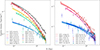 |
Fig. B.1. Projected number density profiles, N(R), for all the considered subsamples of galaxy populations after stacking. In the left panel, we show the N(R) of the main galaxy populations (all red galaxies, all blue galaxies, etc), as well as the N(R) of the whole sample of selected cluster members. In the right panel, we show the four subcategories of the main populations (red with high M*, blue with low M*, etc) |
 |
Fig. B.2. Results of the gOM anisotropy model for the major cluster member populations. In the left column, we show the β(r) values, while, on the right one, we plot those of β′(r) = σr/σϑ. The four rows are organised to distinguish the different mass and number density models adopted in each situation, and they are specified on the label of each vertical axis. The shadowed region represents the 1σ confidence interval, while the yellow line represents the R200c of the stacked cluster. |
 |
Fig. B.3. Results of the gT anisotropy model for the major cluster member populations. See Fig. B.2 for further details. |
 |
Fig. B.4. Results of the gOM anisotropy model for the minor cluster member populations. See Fig. B.2 for further details. |
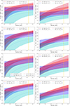 |
Fig. B.5. Results of the gT anisotropy model for the minor cluster member populations. See Fig. B.2 for further details. |
Best-fit values of β0 and β∞ for the major galaxy populations.
Best-fit values of β0 and β∞ for the minor galaxy populations.
Appendix C: JE full results and error dissection plots
In Fig. C.1 we report the full set of results for the JI analysis. We analyse the JI total error budget by splitting the systematic and the statistical components. For the systematics, we compute 250 alternative β(r) profiles by varying the values of the set of arbitrarily chosen parameters: we extract from a uniform distribution the values of ξ, f, Rinf, and the smoothing factors for N(R) and σlos(R), while we extract the values of the total mass profile scale radius from a Gaussian distribution, centred on the best-fit value of the scale radius and with the error on such scale radius as its standard deviation. For the statistical errors, we generate 250 new N(R) and σlos(R) profiles through a bootstrap technique, and, consequently, we compute the corresponding β(r) profiles. Finally, to evaluate the general (statistical + systematics) confidence intervals, we compute 250 alternative β(r) profiles made by picking N(R) and σlos(R) from the bootstrapped sample and by extracting the arbitrary parameters from their assigned distribution. For all of these sets of β(r), we take the interval between the 16th and the 84th percentile of the values of the newly generated β(r) at every radius, and we consider it as the 1σ confidence interval of that kind of error. An example of his operation is shown in Fig. C.2.
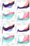 |
Fig. C.1. Results of the JI method for all cluster member populations. In the left column, we show the β(r) values, while on the right one we plot those of β′(r) = σr/σϑ. In the upper half of this figure (see label of each vertical axis), results are based on a NFW total mass profile, while in the lower half on Hernquist profile. The shaded regions represent the 1σ confidence intervals (see Sect. 7.4.1 for further details), while the yellow line represents the R200c of the stacked cluster. |
 |
Fig. C.2. Dissection of the JI confidence intervals for the whole HM galaxy population (see Sect. 7.4.1). The dashed green lines represent the systematic uncertainty, while the dashed blue lines represent the uncertainty from bootstrapping both N(R) and σlos(R). The dashed red lines and the red shaded region mark the overall 1σ confidence interval. The vertical black line represents the R200c of the stacked cluster. |
All Tables
All Figures
|
Fig. 1. Membership selection with CLUMPS on the PPS for the cluster M1115. The green dots represent the galaxy cluster members, while the red dots represent background and foreground galaxies. |
| In the text | |
|
Fig. 2. Colour subdivision for the members of M0329, both on the colour-colour plane (V−I versus B−R; left panel) and on the R-band magnitude versus B−R colour plane (right panel). The latter is the plot used to determine which galaxies are red and which are not, according to the recursive red sequence linear fit. The “all-matched” entry in the legend, corresponding to the yellow points, represents the objects in the photometric catalogue that have a match in the spectroscopic catalogue. |
| In the text | |
|
Fig. 3. PPS of major cluster-member populations of this work, re-scaled by the mean value of R200c and v200. The scale at the right of every plot represents the number of objects in each bin. We note that the blue galaxies, as expected, are more concentrated towards the outer regions of our ensemble cluster, while the red ones are mostly found in the inner regions. The HM population, despite it being radially distributed almost the same as the LM population, is slightly less spread out in terms of velocity than the latter. |
| In the text | |
|
Fig. 4. Comparison between β(r) profiles from the two methods of the whole cluster member population. In the left panel, we plot all the MAMPOSSt outcomes with an NFW total mass profile, as well as both the JI results (NFW and Hernquist) for reference. In the right panel, similarly, we plot all the MAMPOSSt outcomes with a Hernquist total mass profile. The vertical black line represents the R200c of the stacked cluster. |
| In the text | |
|
Fig. A.1. Colour cuts operated on the AS1063 catalogues. In the left panel, we report the first cut (grey region marked by black boundaries) in the colour-colour plane V−I versus B−R. In the right panel, we report the cut (second cut), operated in the R band magnitude versus B−R colour plane, of the subsample extracted from the first cut. The selected objects in this panel are those above the black line. The "all-matched" entry in the legend, corresponding to the red points, indicates the objects in the photometric catalogue that have a match in the spectroscopic catalogue. |
| In the text | |
|
Fig. B.1. Projected number density profiles, N(R), for all the considered subsamples of galaxy populations after stacking. In the left panel, we show the N(R) of the main galaxy populations (all red galaxies, all blue galaxies, etc), as well as the N(R) of the whole sample of selected cluster members. In the right panel, we show the four subcategories of the main populations (red with high M*, blue with low M*, etc) |
| In the text | |
|
Fig. B.2. Results of the gOM anisotropy model for the major cluster member populations. In the left column, we show the β(r) values, while, on the right one, we plot those of β′(r) = σr/σϑ. The four rows are organised to distinguish the different mass and number density models adopted in each situation, and they are specified on the label of each vertical axis. The shadowed region represents the 1σ confidence interval, while the yellow line represents the R200c of the stacked cluster. |
| In the text | |
|
Fig. B.3. Results of the gT anisotropy model for the major cluster member populations. See Fig. B.2 for further details. |
| In the text | |
|
Fig. B.4. Results of the gOM anisotropy model for the minor cluster member populations. See Fig. B.2 for further details. |
| In the text | |
|
Fig. B.5. Results of the gT anisotropy model for the minor cluster member populations. See Fig. B.2 for further details. |
| In the text | |
|
Fig. C.1. Results of the JI method for all cluster member populations. In the left column, we show the β(r) values, while on the right one we plot those of β′(r) = σr/σϑ. In the upper half of this figure (see label of each vertical axis), results are based on a NFW total mass profile, while in the lower half on Hernquist profile. The shaded regions represent the 1σ confidence intervals (see Sect. 7.4.1 for further details), while the yellow line represents the R200c of the stacked cluster. |
| In the text | |
|
Fig. C.2. Dissection of the JI confidence intervals for the whole HM galaxy population (see Sect. 7.4.1). The dashed green lines represent the systematic uncertainty, while the dashed blue lines represent the uncertainty from bootstrapping both N(R) and σlos(R). The dashed red lines and the red shaded region mark the overall 1σ confidence interval. The vertical black line represents the R200c of the stacked cluster. |
| In the text | |
Current usage metrics show cumulative count of Article Views (full-text article views including HTML views, PDF and ePub downloads, according to the available data) and Abstracts Views on Vision4Press platform.
Data correspond to usage on the plateform after 2015. The current usage metrics is available 48-96 hours after online publication and is updated daily on week days.
Initial download of the metrics may take a while.