| Issue |
A&A
Volume 707, March 2026
|
|
|---|---|---|
| Article Number | A153 | |
| Number of page(s) | 15 | |
| Section | Cosmology (including clusters of galaxies) | |
| DOI | https://doi.org/10.1051/0004-6361/202555439 | |
| Published online | 03 March 2026 | |
CLASH-VLT: The variance in the velocity anisotropy profiles of galaxy clusters
1
INAF-Osservatorio Astronomico di Trieste Via G. B. Tiepolo 11 34143 Trieste, Italy
2
IFPU-Institute for Fundamental Physics of the Universe Via Beirut 2 34014 Trieste, Italy
3
Dipartimento di Fisica, Università degli Studi di Milano Via Celoria 16 I-20133 Milano, Italy
4
Dipartimento di Fisica G. Occhialini, Università degli Studi di Milano-Bicocca Piazza della Scienza 3 I-20126 Milano, Italy
5
Department of Physics and Earth Sciences, University of Ferrara, Via G. Saragat 1 44122 Ferrara, Italy
6
Dipartimento di Fisica E. R. Caianiello, Università Degli Studi di Salerno Via Giovanni Paolo II I-84084 Fisciano (SA), Italy
7
INAF – Osservatorio Astronomico di Capodimonte Via Moiariello 16 I-80131 Napoli, Italy
8
IATE – Instituto de Astronomía Teórica y Experimental, Consejo Nacional de Investigaciones Científicas y Técnicas de la República Argentina (CONICET), Universidad Nacional de Córdoba Laprida 854 X5000BGR Córdoba, Argentina
9
INAF – IASF Milano Via A. Corti 12 I-20133 Milano, Italy
10
Dipartimento di Fisica dell’Università degli Studi di Trieste – Sezione di Astronomia Via Tiepolo 11 I-34143 Trieste, Italy
11
University Observatory, Ludwig-Maximilians University Munich Scheinerstrasse 1 81679 Munich, Germany
12
Centro de Astrobiología (CAB), CSIC-INTA Ctra. de Ajalvir km 4 Torrejón de Ardoz 28850 Madrid, Spain
★ Corresponding author: This email address is being protected from spambots. You need JavaScript enabled to view it.
Received:
8
May
2025
Accepted:
31
January
2026
Abstract
Context. The velocity anisotropy profiles, β(r), of galaxy clusters are directly related to the shape of the orbits of their member galaxies. Knowledge of β(r) is important in order to understand the assembly process of clusters and the evolutionary processes of their galaxies, and to improve the determination of cluster masses based on cluster kinematics.
Aims. We determined the β(r) of nine massive clusters at redshift 0.19 ≤ z ≤ 0.45 from the CLASH-VLT dataset, with ≃150–950 spectroscopic members each, to understand how much cluster-to-cluster variance exists in the β(r) of different clusters and what the main driver of this variance is.
Methods. We selected spectroscopic cluster members with the CLUMPS algorithm calibrated on cosmological simulations. We applied the MAMPOSSt code to the distribution of cluster members in projected phase-space to constrain the cluster mass profile, M(r), using priors derived from a previous gravitational lensing analysis. Given the MAMPOSSt best-fit solution for M(r), we then solved the inversion of the Jeans equation to determine β(r) without assumptions of its functional form. We also ran the DS+ code to identify subclusters and characterize the dynamical status of our clusters.
Results. The average ⟨β(r)⟩ is slightly radial; the anisotropy increases from β ≃ 0.2 at the cluster center to β ≃ 0.5 at the virial radius. There is substantial variance in the β(r) of the individual clusters that cannot be entirely accounted for by the observational uncertainties. Clusters of lower mass and with a low concentration per given mass have more tangential β(r) profiles. A comparison with previous works in the literature suggests that orbits are more radial in clusters at higher z. A comparison with cluster-sized halos in cosmological hydrodynamical simulations indicates a very good agreement for the average ⟨β(r)⟩, but a smaller variance in the profiles than observed.
Conclusions. Massive clusters cannot be characterized by a unique universal β(r). The orbital distribution of cluster galaxies carries information on the merging history of the cluster.
Key words: galaxies: clusters: general / galaxies: evolution / galaxies: kinematics and dynamics
© The Authors 2026
 Open Access article, published by EDP Sciences, under the terms of the Creative Commons Attribution License (https://creativecommons.org/licenses/by/4.0), which permits unrestricted use, distribution, and reproduction in any medium, provided the original work is properly cited.
This article is published in open access under the Subscribe to Open model. This email address is being protected from spambots. You need JavaScript enabled to view it. to support open access publication.
1. Introduction
Determining the orbits of galaxies in clusters is useful in order to understand the evolution of clusters themselves. The initial evolution of clusters is thought to be characterized by the violent relaxation process (Lynden-Bell 1967) that isotropizes galaxy orbits. Violent relaxation is also expected to occur during major mergers of clusters (Valluri et al. 2007). Since most major mergers occur with a nonzero impact parameter, transfer of the angular momentum of the secondary cluster to individual galaxies may lead to an excess of tangential orbits. In contrast, smooth accretion of galaxies from the field is instead characterized by more radially elongated orbits (Lapi & Cavaliere 2011). Determining the orbits of galaxies in clusters of different masses, in different dynamical states, and at different redshifts can then in principle allow us to trace the average formation and accretion history of clusters. Moreover, galaxies are affected by different processes as they travel across a cluster. For instance, galaxies with orbits that do not come close to the cluster center are more likely to survive several pericenter passages and avoid tidal stripping by the gravitational potential of the cluster and/or gas removal by ram pressure, and they would also experience less encounters with other cluster members (see, e.g., Lotz et al. 2019; Tonnesen 2019).
The most common way to characterize the orbit of galaxies in clusters in observations is through the velocity anisotropy profile β(r),
 (1)
(1)
where ⟨vr2⟩ is the mean squared radial velocity, and ⟨vθ2⟩ and ⟨vϕ2⟩ are the mean squared velocity components along the two tangential directions. Observations indicate that rotational support is significant only for a minority of clusters (Manolopoulou & Plionis 2017; Bartalesi et al. 2025), so it is customary to assume no meridional streaming motions or rotation, which imply ⟨vθ2⟩ = σθ2 and ⟨vϕ2⟩ = σϕ2, and by symmetry, σϕ = σθ. However, radial streaming motions cannot be excluded, for instance due to infall of galaxies from the field. Radial, isotropic, and circular orbits correspond to β = 1, 0, and −∞, respectively. To symmetrize the range of parameter values for radial versus tangential orbits, Mamon et al. (2019) introduced the new variable βsym,
 (2)
(2)
such that radial, isotropic, and circular orbits correspond to βsym = 2, 0, and −2, respectively.
The velocity anisotropy profile β(r) enters the Jeans equation of dynamical equilibrium (e.g., Binney & Tremaine 1987),
 (3)
(3)
where M(r) is the cluster total mass profile and ν(r) is the number density profile of the tracer of the gravitational potential. Assuming spherical symmetry, ν(r) can be derived from the observed projected number density profile, N(R), of the tracer, via the Abel deprojection. However, it is impossible to infer both M(r) and β(r) from the observed line-of-sight (los) velocity dispersion profile (VDP). This is called the mass-anisotropy degeneracy in the Jeans equation, which can be broken if M(r) is determined with other independent probes than cluster kinematics, such as gravitational lensing and the application of the hydrostatic equilibrium to the intracluster X-ray emitting gas (see, e.g., Natarajan & Kneib 1996; Benatov et al. 2006; Hwang & Lee 2008; Biviano et al. 2013; Munari et al. 2014; Annunziatella et al. 2016; Aguerri et al. 2017).
In the absence of an external determination of M(r), the mass-anisotropy degeneracy can be at least partially solved by considering the entire velocity distribution of the tracers rather than restricting the analysis to the los VDP, as first pointed out by Merritt (1987). Łokas & Mamon (2003) used the kurtosis profile of the velocity distribution of Coma cluster galaxies, in addition to the los VDP, to infer mostly isotropic orbits for its member galaxies. Their method was validated by Sanchis et al. (2004), using cosmological N-body simulations. Wojtak et al. (2008, 2009) constructed distribution function models for the energy and angular momentum of the system to constrain the orbital distribution of cluster galaxies by using their full projected phase-space distribution. Wojtak & Łokas (2010) applied this method to nearby clusters and found an average β(r) close to isotropic near the center and mildly more radial outside, but with substantial variance from cluster to cluster.
Another method that uses the full projected phase-space distribution of cluster galaxies to infer β(r) and at the same time M(r) is MAMPOSSt1 (Mamon et al. 2013). In MAMPOSSt the distribution function is no longer expressed in terms of energy and angular momentum, but in terms of the three-dimensional velocity distribution function, assumed to be Gaussian. Using parametric forms for M(r) and β(r), MAMPOSSt solves the Jeans Eq. (3) to compute the likelihood of the distribution of tracers in projected phase-space. MAMPOSSt has been validated with N-body cosmological simulations (Mamon et al. 2013; Aguirre Tagliaferro et al. 2021; Read et al. 2021).
Similarly to what was found by the distribution function method of Wojtak & Łokas (2010), the MAMPOSSt-based studies found nearly isotropic orbits near the cluster center and increasingly radial orbits at larger cluster-centric distances. Red and blue galaxies share a similar orbital distribution in z ≳ 0.2 clusters (Biviano et al. 2013; Mercurio et al. 2021; Biviano et al. 2016, 2017; Capasso et al. 2019), while in low-z clusters the orbits of early-type galaxies are less radial than those of late-type galaxies (Mamon et al. 2019; Valk & Rembold 2025). Extremely elongated radial orbits characterize galaxies subjected to ram-pressure stripping (Biviano et al. 2024). Galaxies in fossil systems appear to be characterized by more radially elongated orbits than their counterparts in normal clusters (Zarattini et al. 2021).
Another way to at least partially solve the mass anisotropy degeneracy is to use several independent tracers of the same potential (Battaglia et al. 2008). Biviano & Katgert (2004) adopted the M(r) derived by Katgert et al. (2004), who used only early-type galaxies as tracers, to invert the Jeans equation by the method of Solanes & Salvador-Solé (1990, first developed by Binney & Mamon 1982), and determined β(r) for the cluster galaxy populations that were not used in the determination of M(r). By a similar approach, Adami et al. (2009) determined β for dwarf galaxies in Coma, adopting the M(r) derived by Geller et al. (1999), who used bright galaxies as tracers. Biviano & Poggianti (2009) solved the Jeans equation separately for passively evolving galaxies and emission line galaxies in two stacks of clusters at mean redshifts of 0.07 and 0.56, and found suggestive evidence of the orbital evolution of the passive galaxies from radial to isotropic with decreasing z.
Due to the lack of sufficient statistics for each individual cluster, to date most cluster β(r) determinations have been based on stacked samples (Biviano & Katgert 2003; Biviano & Poggianti 2009; Biviano et al. 2016, 2017; Capasso et al. 2019; Mamon et al. 2019). Individual cluster studies show a variety of β(r) (Natarajan & Kneib 1996; Łokas & Mamon 2003; Benatov et al. 2006; Hwang & Lee 2008; Biviano et al. 2013; Munari et al. 2014; Annunziatella et al. 2016; Aguerri et al. 2017; Mercurio et al. 2021), but it is difficult to know how much of this variance is due to the different methodological approaches used by the different authors. Nevertheless, significant β(r) variance is also found in two studies that have determined β(r) for several clusters in homogeneous ways, those of Wojtak & Łokas (2010, 41 z < 0.1 clusters with ≥66 members each) and Li et al. (2023, ten z < 0.1 clusters with ≥75 members each).
The aim of this paper is to better constrain the cluster-to-cluster variance in β(r), using a sample of nine very massive clusters (M2002 > 0.7 × 10¹⁵ M⊙) located at higher z (0.19 − 0.45) than the clusters analyzed by Wojtak & Łokas (2010) and Li et al. (2023). Our nine clusters are part of the CLASH-VLT sample (Rosati et al. 2014, Rosati et al., in prep.), each with ≃150 to 950 spectroscopic members in the virial region, thus allowing the determination of β(r) with much better statistics than the previous studies. In our analysis we first determine the nine cluster M(r) profiles with MAMPOSSt, using priors obtained from gravitational lensing (Umetsu et al. 2018, U18 hereafter), and then invert the Jeans equation by the technique of Solanes & Salvador-Solé (1990) and Dejonghe & Merritt (1992) to determine the individual cluster β(r) profiles and a weighted mean of these profiles. We find significant variance in the individual β(r) profiles, and try to understand its origin by correlating β(r) deviations from the mean with other cluster properties. We compare our results with the β(r) of halos in two cosmological simulations, and with the results of Wojtak & Łokas (2010) and Li et al. (2023) for nearby clusters.
The structure of this paper is as follows. In Sect. 2 we describe the dataset, and in Sect. 3 the method of analysis. In Sect. 4 we present our results, the β(r) of the nine clusters, and their weighted average. We then explore the correlations between the β(r) deviations from the average and other cluster properties, and compare our results to those of Wojtak & Łokas (2010) and Li et al. (2023) at lower z, and to the β(r) of halos from cosmological simulations. In Sect. 5 we discuss our results and in Sect. 6 we provide our summary and conclusions. Throughout this paper we assume a ΛCDM cosmology with Ωm, 0 = 0.3, ΩΛ, 0 = 0.7, and H0 = 70 km s−1 Mpc−1.
2. The dataset
Our dataset consists of nine massive galaxy clusters (M200 > 0.7 × 10¹⁵ M⊙) at intermediate redshifts (0.19 ≲ z ≤ 0.44) from the Cluster Lensing And Supernova survey with Hubble (CLASH; see Postman et al. 2012), with extensive spectroscopic follow-up at the ESO VLT (the CLASH-VLT sample; Rosati et al. 2014, Rosati et al. in prep.). In Table 1 we list these nine cluster identification names, the short names we use in this paper, their center coordinates, and mean z. These nine clusters are a subset of the original CLASH-VLT sample of 13. The excluded clusters are MACS1311.0−0310 because it does not have a M(r) determination by the gravitational lensing analysis of U18; MACS0416.1−2403 because it is a merging cluster with a very complex dynamical state (Balestra et al. 2016), which probably invalidates the application of the Jeans equation; RXJ1347.5−1145 because it lacks complete photometric coverage to fully assess its spectroscopic completeness; and MACS2129.4−0741 because of insufficient spectroscopic data.
Cluster sample.
In Table 1 we also list the number of spectroscopic members in the virial region used in the dynamical analysis of this paper (Nm, see below for the membership definition), and brighter than the R-band magnitude limits, mR, lim, listed in Table 1. These magnitude limits were set to ensure a spectroscopic completeness ≥30% throughout the whole virial region. The completeness estimates are described in Maraboli et al. (in prep.). They are based on color–color cuts in the mB − mR versus mV − mI plane that allow both red and blue cluster galaxies to be included, and on color–magnitude cuts in the B − R versus R plane that allow low-z bright nonmembers to be rejected. Previous works exploring the dynamics of CLASH-VLT clusters (Annunziatella et al. 2016; Sartoris et al. 2020; Mercurio et al. 2021; Biviano et al. 2023; Girardi et al. 2024) quote larger numbers of spectroscopic members since they did not apply these color and magnitude cuts to the sample. Finally, in Table 1 we list the U18 estimates of their virial and scale radius, r200 and rs, that we computed from the values of M200 and c2003 listed in Table 1 of U18.
Photometric data were obtained with the Suprime-Cam imager (Miyazaki et al. 2002) at the Subaru telescope, for all nine clusters except for R2248, which was observed with the Wide-Field Imager at the ESO 2.2 m MPG / ESO telescope (Gruen et al. 2013; Mercurio et al. 2021). We refer to Umetsu et al. (2014, Sect. 4.2 and Tables 1 and 2) for a detailed description of the available multiband images for each of the nine clusters.
The spectroscopic data come mostly from the CLASH-VLT program4 (Rosati et al. 2014, Rosati et al. in prep.), and were obtained with the VIsual Multi-Object Spectrograph (VIMOS, Le Fèvre et al. 2003). Part of these spectroscopic data have already been released (see Annunziatella et al. 2016 for A209, Biviano et al. 2013; Caminha et al. 2017 for M1206, and Karman et al. 2017; Mercurio et al. 2021 for R2248). Additional spectroscopy, deeper but in smaller fields, has been obtained for some of our clusters with the Multi Unit Spectroscopic Explorer (MUSE, Bacon et al. 2010). The full spectroscopic dataset contains 24 100 high-quality z values. Further details on the photometric and spectroscopic datasets are given in Maraboli et al. (in prep.).
3. Analysis
In our analysis we adopt the spherical approximation. Although clusters are not spherically symmetric, this is a necessary approximation if we want to solve the spherical Jeans equation. Going beyond the spherical approximation requires introducing other parameters that are impossible to tightly constrain even with the unprecedented amount of spectroscopic data available for our dataset. As we discuss in Sect. 4.3, we adopt the same spherical approximation to derive the β(r) of cluster-size halos from numerical simulations, to allow a proper comparison with our results. However, the spherical approximation was not adopted in the gravitational lensing analysis of U18, who modeled the cluster mass profiles with elliptical NFW (Navarro et al. 1996, 1997) models. Since we used the values derived from U18 for M200 and c200 as priors in our dynamical analysis with MAMPOSSt, we compared the elliptical 3D mass profiles of U18 with the 3D mass profiles derived by the gravitational lensing analysis of Umetsu et al. (2014) under the spherical approximation. Specifically, we computed the ratios of these elliptical and spherical mass profiles, Me/Ms, at three different overdensities, Δ = 500, 200, and 100. We found an average Me/Ms = 0.97 over the nine clusters in our sample, the same value at all Δ values. The rms of these ratios are 0.08, 0.13, and 0.17 at Δ = 500, 200, and 100, respectively. For none of our nine clusters does the Me/Ms ratio differ from unity at more than 1.6σ at any Δ. We conclude from this analysis that the spherical approximation does not cause significant differences in the lensing M(r) determinations.
Since our analysis is based on the Jeans equation, we also implicitly assume dynamical equilibrium, a valid assumption if the number of galaxies in any given region of the cluster phase-space does not change. Rapid mass growth of a cluster can invalidate this assumption. Based on the predictions of the theoretical model by Li et al. (2007), it is expected that a cluster with the mean mass and the mean redshift of our sample has grown in mass by ∼20% over the past ∼1 Gyr, which is the dynamical time of the cluster (Sarazin 1986). This is not entirely negligible, and given the substantial variance in the mass accretion history of different halos of similar mass, we cannot exclude that some of our clusters depart from dynamical equilibrium due to a recent major merger. We come back to this question in Sect. 4.1 when we consider the possible effect of rich subclusters on the β(r).
Since accretion is most likely to occur inside-out, in order to minimize its effect on the cluster dynamical state we restricted our dynamical analysis to the R ≤ 1.36 r200 region. At the mean z = 0.32 of our clusters, 1.36 r200 is between the virial radius ∼r126 ≈ 1.22 r200 (Bryan & Norman 1998), and the splashback radius ∼1.5 r200, within which the cluster dynamics is still dominated by galaxies orbiting the cluster potential (Pizzardo et al. 2024). We also excluded the central 50 kpc region from our analysis since this region is dominated by the gravitational potential of the brightest cluster galaxy, so the total M(r) deviates from the NFW model (see, e.g., Biviano & Salucci 2006; Mamon et al. 2019; Sartoris et al. 2020).
3.1. Cluster membership
We used the CLUster Membership in Phase Space (CLUMPS) method of Biviano et al. (2021) to establish cluster membership, with parameters calibrated on light cones constructed from GAEA mocks (De Lucia et al. 2024). The GAlaxy Evolution and Assembly (GAEA) semi-analytical model is a substantial update of the model of De Lucia & Blaizot (2007), and is based on the Millennium simulation (Springel et al. 2005). We considered the 358 richest halos with more than 150 members to mimic the richness distribution of our nine clusters. We calibrated the CLUMPS parameters, dR, and dV to optimize the membership completeness and purity of simulated galaxies in halos. We found that dR = 450 kpc and dV = 200 km s−1 give an average membership completeness > 0.99 and a purity > 0.85. The values of the CLUMPS parameters we find differ from those recommended by Biviano et al. (2021), but in that study the mock sample contained halos with as few as ten members.
We ran CLUMPS on our nine clusters, using the positions of their BCG as a center (the BCG coordinates are given in Table 1). After running CLUMPS we further refined the membership selection by taking advantage of the fact that we already had good estimates of the cluster M(r) from the gravitational lensing analysis of U18. Given M(R), we computed the escape velocity vesc(R) as a function of projected radius, R, by considering a wide range of possible β(r). Specifically, we considered two models:
 (4)
(4)
with δ = 1 (generalized Tiret model, gT hereafter Tiret et al. 2007) and δ = 2 (generalized Osipkov-Merritt model, gOM hereafter Osipkov 1979; Merritt 1985), where we forced rβ ≡ rs, based on the results of numerical simulations (Mamon et al. 2010), to limit the number of free parameters. For each of the two models, we considered three values for β0, −99, 0, and 0.99 (which correspond to βsym values of −1.96, 0, and 1.96, respectively) and the same three values for β∞, for a total of 18 profiles. For each of these β(r), we calculated vesc(R) and excluded from the sample of cluster members any galaxy with a los velocity in the cluster rest-frame, |vrf|> max(vesc(R)), where max(vesc(R)) is the largest escape velocity at the galaxy projected radius, R, among the 18 considered. This procedure ensured that we removed any remaining interlopers after the CLUMPS selection in a conservative way, without biasing our results, given the extremely wide range of β(r) considered. On average, this additional membership selection removed only 4% of the galaxies initially identified as members by CLUMPS.
In Fig. 1 we show the distribution in projected phase-space of member galaxies in the cluster M1206, selected by the CLUMPS algorithm and by the vesc(R) condition (all nine clusters are shown in Fig. A.1). In Table 1 we list the number of members Nm selected by CLUMPS and by the vesc(R) condition, in the radial range we consider in our dynamical analysis, i.e., from 50 kpc to 1.36 r200, where r200 comes from U18.
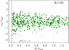 |
Fig. 1. Projected phase-space diagram of the 427 galaxies selected as members of the M1206 cluster (other clusters are shown in Fig. A.1) by the CLUMPS method in the region R ≤ 1.36 r200. The three numbers at the bottom left indicate, from left to right, the number of galaxies selected for the dynamical analysis (black-circled green dots); the number of CLUMPS members that are excluded from the dynamical analysis because they are at R ≤ 0.05 Mpc, which is the region dynamically dominated by the BCG (red circles), and the number of CLUMPS members that are not used in the dynamical analysis because they are flagged as interlopers by the escape-velocity criterion (gray circles). The vertical lines indicate R = 0.05 Mpc and R = r200. The values of r200 and v200 come from U18. |
Previous dynamical analysis were conducted on four of the nine clusters in our sample, based on the same dataset, but using different membership selection techniques, and no magnitude cut (Biviano et al. 2013; Annunziatella et al. 2016; Sartoris et al. 2020; Mercurio et al. 2021; Girardi et al. 2024). In Fig. A.2 we show that the different membership selections do not significantly modify the los velocity dispersion profiles of these four clusters. This suggests that our results are stable versus different membership selections.
3.2. Number density profiles
The 3D number density profile of cluster members, ν(r), enters the Jeans Eq. (3). Under the spherical assumption, this can be directly obtained from the projected number density profile, N(R), via the Abel inversion (see, e.g., Binney & Tremaine 1987). We determine N(R) using the radial distribution of cluster members after correcting for spectroscopic incompleteness, as described in Maraboli et al. (in prep.). We determine N(R) in  bins, where Nm is the number of cluster members in the radial range 0.05 Mpc ≤ R ≤ 1.36 r200, with r200 from U18. This binned profile is used in the Jeans Equation Inversion (JEI) analysis described in Sect. 3.3. We also provide model fits to the N(R) using a maximum likelihood procedure that does not require binning. We consider two models, NFW (in projection, see Bartelmann 1996) and King (1962), each characterized by just one free parameter, the scale radius rν. The normalization of N(R) is not a free parameter in the fit since it is set by the requirement that the integrated profile corresponds to the number of cluster members corrected for incompleteness.
We list in Table 2 the best-fit models and scale radii for our nine clusters. Only in one case (A209) is the King model, characterized by a central core, a better fit to N(R) than the NFW model. In all cases the models provide acceptable fits to the observed profiles, within the 90% confidence level, according to a χ2 test.
Results from the N(R) fits and MAMPOSSt.
3.3. Solving the Jeans Equation for β(r)
To determine β(r) from the observables, we first need to break the Jeans equation degeneracy using a M(r) estimate. For this we use the MAMPOSSt method of Mamon et al. (2013) applied to the phase-space distribution of cluster members, using the public code MG-MAMPOSSt (Pizzuti et al. 2023). MAMPOSSt estimates the probability of finding a cluster galaxy at its observed position in projected phase-space, for a set of M(r) and β(r) model parameters, by solving the spherical Jeans equation, under the assumption of a Gaussian 3D velocity distribution. The best-fit M(r) and β(r) parameters are found by maximizing the product of the individual galaxy probabilities. To improve the uncertainties in the posteriors of the MAMPOSSt analysis we adopted the M(r) estimate by U18 as priors whenever possible, that is, for eight of our nine clusters, as described below.
In a first iteration we ran MAMPOSSt by adopting the NFW model for M(r), using flat priors on the r200 and rs parameters in the ranges 1.0–3.0 and 0.2-2.0 Mpc, respectively. We used a Gaussian prior for the scale parameter of the ν(r) profile, rν, with a mean and 1σ error obtained from the maximum likelihood fit to the completeness-corrected N(R) (see Sect. 3.2 and Table 1). We considered two β(r) models, gT and gOM (see eq. 4) with flat priors on their β0, β∞ parameters in the range −3 to 0.96 (which corresponds to βsym values of −1.2 and 1.85, respectively). We then ran a Markov chain Monte Carlo (MCMC) procedure with 25 000 steps per cluster, using the Gelman & Rubin (1992) criterion to check for convergence, adopting a threshold of  for the Gelman-Rubin coefficient.
We find that the posteriors for r200 and rs obtained with MAMPOSSt are in agreement at better than 1.5σ with the values given by U18 (and listed in Table 1) for eight of our nine clusters. For M1115 we find a best-fit value of  Mpc, different from the U18 value at 2.5σ and in better agreement with the results of the X-ray analysis of Donahue et al. (2014). For the remaining eight clusters we ran the MAMPOSSt analysis a second time, this time using Gaussian priors on the r200 and rs parameters with mean and 1σ uncertainties as given by U18 (and listed in Table 1).
The resulting best-fit parameters and their 1σ marginalized errors are listed in Table 2. For the β(r) profiles we list the values of βsym at r = 0.05 Mpc and r200 since they are more directly comparable to previous results than the β0, β∞ parameters. The β(r) profiles of the clusters A209, M1206, and R2248 are consistent with the previous MAMPOSSt determinations by Annunziatella et al. (2016), Biviano et al. (2013), and Mercurio et al. (2021), respectively.
The best fit is not necessarily an acceptable fit to the data; to check MAMPOSSt best-fit solutions, we compared them to the observables, the los VDP in this case, evaluated in seven radial bins. The χ2 values of this comparison are given in Table 2. They are computed as
 (5)
(5)
where Δσlos, i is the difference between the observed and predicted los velocity dispersion at the radial bin i, and δσ, i is the observational uncertainty on the observed velocity dispersion. The comparison between predicted and observed VDPs is shown in Fig. 2 for the cluster M1206 as an example; all nine clusters are shown in Fig. A.3.
 |
Fig. 2. Dots with 1σ error bars: los VDP of M1206. Dashed blue line and cyan shading: Best-fit MAMPOSSt solution within 68% confidence levels, estimated on a random selection of 3000 MCMC steps. Red solid line and orange shading: JEI-predicted VDP and 68% confidence levels. The values of r200 (indicated by the vertical magenta line) and v200 are the best fits of the MAMPOSSt analysis (other clusters are shown in Fig. A.3.) |
MAMPOSSt results were not obtained by fitting directly the VDP, so we do not expect perfect agreement, and yet the χ2 values of two clusters (A209 and R2129) are rather high. This could either indicate violation of the dynamical equilibrium condition or that the chosen β(r) models are too rigid to represent the real β(r). While there is a large consensus on the fact that the NFW model is a good representation of M(r) on the cluster scale, at least in the radial range considered in this work, no claim for the universality of β(r) has ever been made. For this reason, we proceeded with the second part of our analysis to determine β(r) free of model assumptions, using the JEI method.
The JEI method solves the Jeans equation for β(r), given M(r). It was first developed by Binney & Mamon (1982); here we followed the implementation of the method by Solanes & Salvador-Solé (1990) and Dejonghe & Merritt (1992). The method we briefly outline here has already been applied to several datasets with small variations (e.g., Biviano & Katgert 2004; Biviano et al. 2013; Annunziatella et al. 2016; Biviano et al. 2016; Zarattini et al. 2021; Biviano et al. 2024).
In our JEI analysis, we adopted the NFW M(r) with the MAMPOSSt best-fit parameters (Table 2). The observables in the JEI method are the binned N(R) (see Sect. 3.2) and the binned VDP (described above). We smoothed both profiles using the LOWESS smoothing technique (see, e.g., Cleveland & McGill 1984; Gebhardt et al. 1994) with a smoothing length of 0.7. We extrapolated the smoothed profiles to large radii (30 Mpc) following Biviano et al. (2013) to allow the equations that contain integrals up to infinity to be solved. The resulting β(r) is a nonparametric profile.
The uncertainties on β(r) are estimated as follows. We run the JEI procedure 1500 times. In each run, we
-
bootstrap resample the projected phase-space (cluster-centric distances and rest-frame velocities), and determine new N(R) and VDP on the bootstrap sample;
-
randomly select the M(r) parameters from one of the MCMC steps of the MAMPOSSt analysis;
-
choose a random value for the LOWESS smoothing parameter between 0.5 and 0.9.
At the end we define the intervals containing 68% of the β(r) profiles at 50 points uniformly spaced in the radial interval analyzed 0.05–1.36 r200. We check for convergence by comparing the 68% confidence region we derive, with that obtained with 1000 runs.
4. Results
In Fig. 2 we show the observed VDP (dots with error bars) and the VDP implied by the JEI procedure for M1206 (and for all nine clusters in Fig. A.3). By construction, the JEI solution for the VDP coincides with the LOWESS smoothed VDP, only if a dynamical equilibrium solution exists for the adopted M(r). This is indeed the case for all nine of our clusters, and it suggests that the not-so-good agreement between the MAMPOSSt and the observed VDPs for some clusters was not due to a violation of dynamical equilibrium, but to the rigidity of the adopted β(r) models. Nonetheless, the MAMPOSStβ(r) are in agreement with the JEIβ(r) within the uncertainties (see Fig. A.4), with the exception of the central region of A209. This difference might be due to the fact that the N(R) models adopted in the MAMPOSSt analysis are not general enough to always fit the observed profiles very closely. It is perhaps worth noting that A209 is the only cluster for which the NFW model does not provide a good fit to the observed N(R).
In Fig. 3 we show the main result of this article, that is, the nine individual βsym(r) obtained with JEI (yellow lines) and the Nm-weighted mean of these profiles (black dash-dotted line),
 |
Fig. 3. Each panel shows the 1σ confidence levels of a cluster JEIβsym(r), as obtained from the procedure described in Sect. 3.3 (red shadings), and its central value (yellow line), the weighted mean of the nine profiles, ⟨βsym(r)⟩, as defined in Eq. (6) (black dash-dotted line), and the βsym(r) of the other eight clusters (black dotted lines). The horizontal dashed black line indicates isotropic orbits. Orbits are radial above this line and tangential below it. |
 (6)
(6)
The red shadings indicate the 1σ uncertainties on the individual cluster β(r) obtained from the bootstrap analysis described in Sect. 3.3.
Despite the large uncertainties, there are significant differences among the different cluster β(r) profiles. This indicates that there is no universal β(r) for galaxy clusters. In this respect, the average ⟨β(r)⟩ is not representative of the whole cluster population and we use it just as a reference. In the following, we investigate the possible causes of the different β(r).
4.1. Correlation with other cluster properties
We define the deviation of the individual cluster βsym(r) from their weighted average as
 (7)
(7)
where the βsym profiles are evaluated in 50 equally spaced radial points in the radial range we considered for our analysis (0.05 Mpc to 1.36 r200). We note that the average profile is not representative of the whole cluster population β(r) due to the significant variance from cluster to cluster. Here we use it as a convenient reference profile to quantify the cluster-to-cluster β(r) variations.
Quantities for regression analysis.
We searched for correlations of dβ with the following cluster properties to try to understand the physical reason for the substantial variance in the cluster βsym(r):
-
M200;
-
c200;
-
cν ≡ r200/rν;
-
the total fraction of blue galaxies, fblue;
-
the total fraction of galaxies in subclusters, fsub.
All quantities are listed in Table 3. The quantities M200, c200, cν are the best-fit values obtained in the MAMPOSSt analysis. The total fraction of blue galaxies fb is taken from Maraboli et al. (in prep.). To determine fsub, we ran the DS+ subcluster analysis in its no-overlapping mode (Benavides et al. 2023). DS+ is a development of the method originally proposed by Dressler & Shectman (1988). It examines possible subclusters of different multiplicities around each cluster member, and identifies those with significant different kinematics from the cluster. We were not interested in identifying very small subclusters, but only those that are expected to leave a significant effect on the internal cluster dynamics. We therefore only looked for subclusters richer than Nm/10. To speed up calculations, we did not consider subclusters of all possible multiplicities as in the original DS+ code, but only those with any of six multiplicities equally spaced between Nm/10 and Nm/3. We ran 1000 MonteCarlo resamplings to establish the subcluster probabilities, and retained only those with a formal probability < 1/1000. In Fig. A.5 we show the spatial distributions of the subclusters found in each of our nine clusters.
We performed a stepwise regression analysis to identify the main predictive cluster properties for dβ, using a forward selection approach (Efroymson 1960, see also Biviano et al. 1992, for an astrophysical application of the method). In this procedure, we start by considering the cluster property that is most strongly correlated with dβ and then we continue by adding the variable that contributes the largest increase in the coefficient of determination, R25. In Fig. 4 we show R2 versus the cluster properties. There are two main predictive variables for dβ, namely M200 and c200; other cluster properties contribute very little to the improvement of the regression.
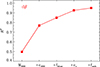 |
Fig. 4. Results of the stepwise regression analysis (forward approach). Each square is the value of the coefficient of determination, R2, of dβ vs. the quantities labeled on the x-axis, with the inclusion of an additional quantity at each new point from left to right. |
A visual confirmation of the results of the stepwise regression analysis is given in Fig. 5 where we show dβ versus M200. The symbol sizes are proportional to c200. There is a clear dependence of dβ on M200, and also on c200 at fixed M200. Clusters of higher mass, and of higher concentration at a given mass, are characterized by more radial orbits.
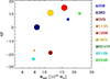 |
Fig. 5. dβ vs. M200. The symbol size is proportional to c200. The colors identify our nine clusters, in order of increasing redshift with increasing color wavelength (from blue to brown). |
4.2. Comparison with previous results
Here we compare our results with those of Wojtak & Łokas (2010) and Li et al. (2023), who have both homogeneously measured β(r) for several clusters. Both studies investigated low-z cluster samples. The Wojtak & Łokas (2010) results were based on modeling the cluster’s energy and angular momentum by distribution function models. Li et al. (2023) solved the Jeans equation using ten free parameters, of which four define the model for β(r) = β0 + (β∞ − β0) [1 + (r0/r)n]−1. To better constrain these parameters, they also used the fourth moment of the los velocity distribution of cluster galaxies.
In Fig. 6 we show βsym(rvir)6 versus the values of βsym estimated at the closest radius to the center of the cluster, βsym(0) for simplicity, for our nine clusters and for the 41 low-z clusters studied by Wojtak & Łokas (2010, we converted the values of β in their Table 2 to βsym). The variance in the values of βsym(rvir) is similar for our sample of clusters and the Wojtak & Łokas (2010) sample. However, the variance in the values of βsym(0) is smaller for our sample since all the clusters in our sample have βsym(0) close to isotropic or slightly radial. In contrast, many of the Wojtak & Łokas (2010) clusters have tangential orbits near the center.
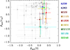 |
Fig. 6. Velocity anisotropy βsym at r = rvir, vs. velocity anisotropy at r = 0, for our nine clusters (colored dots) and for the lower-z clusters of Wojtak & Łokas (2010, black circles). The 1σ error bars are shown. The virial radius is rvir = r100 for the nearby clusters of Wojtak & Łokas (2010), and it is approximated by r126 for our clusters. The colors identify our nine clusters, in order of increasing redshift with increasing color wavelength (from blue to brown). |
In Fig. 7 we show our nine clusters β(r) and their weighted average using the same format and axis ranges of Fig. 4 in Li et al. (2023), to allow a direct comparison with their ten low-z clusters β(r), which we reproduce in our figure. We note that the radii on the x-axis are in units of r500, which we derive using the r200, rs values listed in Table 2, by adopting an NFW mass density profile. The β(r) variance across the clusters in the sample of Li et al. (2023) and in our sample appear similar, but the clusters of Li et al. (2023) have tangential orbits near the center, and a lower degree of radial anisotropy at large radii, compared to our nine clusters.
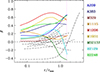 |
Fig. 7. β(r) of our nine clusters (colored solid lines) and of the ten nearby clusters of Li et al. (2023, black dot-dashed lines) displayed in the same format as that of Fig. 4 in Li et al. (2023). The colors identify our nine clusters, in order of increasing redshift with increasing color wavelength (from blue to brown). The vertical magenta dotted line indicates 1.5 r500, which is on average equivalent to r200 for our nine clusters. |
4.3. Comparison with simulations
We here compare the βsym(r) profiles of our nine clusters to those of halos of similar mass and redshifts from cosmological numerical simulations. Specifically, we consider the semi-analytical model GAEA (already used and described in Sect. 3.1) and the hydrodynamical cosmological simulation of Ragone-Figueroa et al. (2018, RF hereafter). The RF simulations have been shown to reproduce well the observational properties of the BCGs, both for their evolution in mass and for their alignment with the host cluster (Ragone-Figueroa et al. 2018, 2020).
We selected 112 halos in the redshift and mass range spanned by our nine clusters, 0.19 ≤ z ≤ 0.45, M200 ≥ 1014.85 M⊙, in GAEA, and 25 halos at z = 0.3, and with M200 ≥ 1014.85 M⊙, in RF. In Fig. 8 we show the βsym(r) profiles of our nine clusters and their weighted mean, and the mean ⟨βsym(r)⟩ and its rms of the selected halos in the GAEA (upper panel) and RF (lower panel) simulations. The GAEA ⟨βsym(r)⟩ lies below the observational mean profile, even if the difference is not statistically significant. On the other hand, the agreement between the RF and observational ⟨βsym(r)⟩ is excellent. The variance in the halo βsym(r) is somewhat larger for the observational sample than for the simulated halos, both in GAEA and RF.
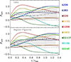 |
Fig. 8. Upper panel: Nine clusters βsym(r) (color-coded in order of increasing redshift with increasing color wavelength, from blue to brown) and their weighted mean velocity anisotropy profile ⟨β(r)⟩ (dash-dotted black line) compared to the mean profile of 112 halos in the GAEA simulation (triple-dot-dashed gray line) and its rms (gray shading). Lower panel: Same as the upper panel, but the comparison is made with the mean profile of 25 halos in the RF simulation. |
The βsym(r) of the simulated halos are direct measurements; we have not tried to mimic the whole observational procedure. The good agreement between the observed and simulated average profiles, if not a pure coincidence, can be considered indirect evidence supporting the reliability of our observational results and the lack of significant systematics in our analysis.
While this paper was being prepared for submission, we became aware of the results of Abdullah et al. (2025), who analyzed β(r) for halos with log M200 ≥ 14.05 up to z = 1.5 in the Uchuu-UM mock catalog of Aung et al. (2023) derived from the Uchuu cosmological N-body simulation (Ishiyama et al. 2021). Their ⟨β(r)⟩ (Fig. 2 in their paper) is completely consistent with our result.
5. Discussion
By our joint lensing, MAMPOSSt, and JEI analysis of our sample of nine clusters, we find that the weighted average β(r) is mildly radially anisotropic at all radii. The radial anisotropy increases with radius up to r200, where it reaches a plateau. There is a significant variance in β(r) from cluster to cluster, even though the nine clusters span a narrow range in mass (M200 ≥ 1014.85 M⊙) and redshift (0.19 ≤ z ≤ 0.45).
A comparison of the average β(r) of our nine clusters with those of halos of similar mass and redshifts from cosmological numerical simulations shows good agreement with the GAEA simulation, and excellent agreement with the RF simulation. However, the β(r) variance appears to be somewhat larger in the observational sample than in the simulated ones. It is possible that the observational variance is inflated by the fact that different clusters are observed at different orientations relative to their major axis, while the β(r) of the simulated halos are averaged over all orientations. We plan to address this point in a future work.
Comparison with previous results in the literature by Wojtak & Łokas (2010) shows that the β(r) variance is higher in nearby clusters than in our cluster sample. This is caused by many nearby clusters showing more tangential orbits near the center than our clusters, as also seen in the sample of nearby clusters of Li et al. (2023). Biviano & Poggianti (2009) were the first to suggest a decreasing radial anisotropy of cluster galaxy orbits with decreasing z. They attributed this orbital evolution to the change in the gravitational potential of the cluster due to the secular growth of the mass of the cluster via hierarchical accretion (Gill et al. 2004) and/or to the mixing of energy and angular momentum that follows episodes of major mergers (Valluri et al. 2007; Lapi & Cavaliere 2011), analogous to the violent relaxation process (Lynden-Bell 1967). An additional physical mechanism that can explain the reduction of radial anisotropy near the cluster center with time is dynamical friction (Chandrasekhar 1943). Even if the timescale for dynamical friction is long for individual galaxies, this process can still be effective for infalling groups (Mamon et al. 2019). The z-evolution of β(r), from more radial to more isotropic orbits with time, is also seen in the Uchuu simulated halos (Abdullah et al. 2025, see their Fig. 4).
We tried to identify the main cluster property that could be responsible for the β(r) variance. We found that higher-M200 clusters, as well as clusters with high c200 at given M200, tend to have more radial orbits. Recently, Pizzuti et al. (2025) have found a similar (but not statistically significant) trend of β(r200) with cluster mass by performing a stacking analysis of 75 z < 0.6 clusters from the CHEX-MATE sample (CHEX-MATE Collaboration 2021).
A trend of increasing β(r200) with halo mass has been observed in cosmological simulations by Munari et al. (2013, see their Fig. 10) and by Abdullah et al. (2025, see their Fig. 3). There is also a trend of the same nature in the RF simulation, with βsym(r200)≈0 for halos with log M200/M⊙ < 14.3, and ≈0.7 for halos with log M200/M⊙ ≥ 14.85. Abdullah et al. (2025) attributes the mass dependence of β(r) to the longer dynamical timescales of more massive halos, requiring more time to reach the more mature dynamical status represented by isotropic orbits. Another possibility is that more massive clusters have a larger fraction of recently accreted galaxies, but we fail to see a significant dependence of β(r) on the fraction of blue galaxies in our sample. On the other hand, orbital isotropization could be caused by major mergers, that induce rapid changes in the cluster gravitational potential, and can temporarily disrupt the central mass distribution, lowering the cluster mass concentration (see, e.g., Okabe et al. 2019; Gianfagna et al. 2023).
In the future, we plan to further investigate this issue, and, more in general, the origin of the variance in cluster β(r) profiles, by following the evolution of the velocity anisotropy profiles of simulated halos in time (Ragone-Figueroa et al., in prep.).
6. Summary and conclusions
We analyzed a sample of nine massive clusters from the CLASH-VLT sample, with M200 ≥ 1014.85 M⊙ and 0.19 ≤ z ≤ 0.45, to determine their velocity anisotropy profiles from the center to slightly beyond the virial radius. We determined the membership of cluster galaxies with an algorithm calibrated on halos from a cosmological simulation. We then used MAMPOSSt to solve the Jeans equation of dynamical equilibrium for the projected phase-space distributions of cluster members. In the MAMPOSSt analysis we adopted the NFW model for M(r), and for eight of our nine clusters, we adopted Gaussian priors on the r200, rs parameters, derived from the gravitational lensing analysis of U18. We then used the MAMPOSSt best fit M(r) in the inversion of the Jeans equation (JEI) to determine β(r) of each individual cluster, without any assumption on the functional form of β(r).
We find that the average ⟨β(r)⟩ of our nine clusters, weighted on the number of cluster members, is radially anisotropic, increasing from β ≃ 0.2 (βsym ≃ 0.25) at the center to β ≃ 0.5 (βsym ≃ 0.66) at r200, and flattening thereafter. The nine cluster β(r) are not all consistent with ⟨β(r)⟩ within their 1σ uncertainties; that is, we detect significance variance in β(r) across the cluster sample. We find that clusters of high mass, and those with a high concentration per given mass, have more radial orbits for their member galaxies. The trend of orbits that are more radial in more massive clusters is also seen in cosmological simulations (Munari et al. 2013; Abdullah et al. 2025), and it is attributed to the longer dynamical timescales of more massive halos. The trend of orbits that are less radial in clusters of lower concentrations could instead be due to major mergers that can cause a decrease in concentration (Okabe et al. 2019; Gianfagna et al. 2023) and, at the same time, lead to the isotropization of the galaxy orbits (Valluri et al. 2007).
A comparison with results from the literature (Wojtak & Łokas 2010; Li et al. 2023), show that clusters at lower z have higher β(r) variance near the center, caused by many clusters in the low-z samples displaying tangential orbits, unlike the nine clusters in our sample that are characterized by mildly radial or isotropic orbits near the center. This orbital evolution with z was already suggested by Biviano & Poggianti (2009). We propose three physical mechanisms that can possibly lead to a reduction in the radial anisotropy of cluster galaxy orbits: (i) dynamical friction (Chandrasekhar 1943; Mamon et al. 2019), (ii) the evolution of the cluster gravitational potential due to mass accretion (Gill et al. 2004), and (iii) violent relaxation following major merger events (Valluri et al. 2007).
We also compared our β(r) to those of halos of similar mass and z, in two cosmological simulations. There is a good agreement of the average β(r) profile with those of the simulated halos, in particular the one from the hydrodynamical simulations of Ragone-Figueroa et al. (2018). In both simulations, the β(r) variance is slightly smaller than the observed one. In the future we plan to investigate the β(r) profiles of cluster-sized halos in hydrodynamical simulations in order to uncover the physical mechanisms affecting the orbits of cluster galaxies (Ragone-Figueroa et al., in prep.).
Acknowledgments
We thank the referee for her/his careful, competent, and useful report, and Gary Mamon and Massimiliano Parente for useful discussion. We acknowledge financial support through the grants PRIN-MIUR 2017WSCC32 and 2020SKSTHZ. AB acknowledges the financial contribution from the INAF mini-grant 1.05.12.04.01 “The dynamics of clusters of galaxies from the projected phase-space distribution of cluster galaxies”. We acknowledge financial support from the European Union’s HORIZON-MSCA-2021-SE-01 Research and Innovation Programme under the Marie Sklodowska-Curie grant agreement number 101086388 – Project (LACEGAL).
References
- Abdullah, M. H., Mabrouk, R. H., Ishiyama, T., et al. 2025, ApJ, 987, 70 [Google Scholar]
- Adami, C., Le Brun, V., Biviano, A., et al. 2009, A&A, 507, 1225 [NASA ADS] [CrossRef] [EDP Sciences] [Google Scholar]
- Aguerri, J. A. L., Agulli, I., Diaferio, A., & Dalla Vecchia, C. 2017, MNRAS, 468, 364 [NASA ADS] [CrossRef] [Google Scholar]
- Aguirre Tagliaferro, T., Biviano, A., De Lucia, G., Munari, E., & Garcia Lambas, D. 2021, A&A, 652, A90 [NASA ADS] [CrossRef] [EDP Sciences] [Google Scholar]
- Annunziatella, M., Mercurio, A., Biviano, A., et al. 2016, A&A, 585, A160 [NASA ADS] [CrossRef] [EDP Sciences] [Google Scholar]
- Aung, H., Nagai, D., Klypin, A., et al. 2023, MNRAS, 519, 1648 [Google Scholar]
- Bacon, R., Accardo, M., Adjali, L., et al. 2010, SPIE Conf. Ser., 7735, 773508 [Google Scholar]
- Balestra, I., Mercurio, A., Sartoris, B., et al. 2016, ApJS, 224, 33 [Google Scholar]
- Bartalesi, T., Ettori, S., & Nipoti, C. 2025, A&A, 697, A17 [NASA ADS] [CrossRef] [EDP Sciences] [Google Scholar]
- Bartelmann, M. 1996, A&A, 313, 697 [NASA ADS] [Google Scholar]
- Battaglia, G., Helmi, A., Tolstoy, E., et al. 2008, ApJ, 681, L13 [NASA ADS] [CrossRef] [Google Scholar]
- Benatov, L., Rines, K., Natarajan, P., Kravtsov, A., & Nagai, D. 2006, MNRAS, 370, 427 [Google Scholar]
- Benavides, J. A., Biviano, A., & Abadi, M. G. 2023, A&A, 669, A147 [NASA ADS] [CrossRef] [EDP Sciences] [Google Scholar]
- Binney, J., & Mamon, G. A. 1982, MNRAS, 200, 361 [Google Scholar]
- Binney, J., & Tremaine, S. 1987, Galactic Dynamics (Princeton, NJ: Princeton University Press), 747 [Google Scholar]
- Biviano, A., & Katgert, P. 2003, Ap&SS, 285, 25 [NASA ADS] [CrossRef] [Google Scholar]
- Biviano, A., & Katgert, P. 2004, A&A, 424, 779 [NASA ADS] [CrossRef] [EDP Sciences] [Google Scholar]
- Biviano, A., & Poggianti, B. M. 2009, A&A, 501, 419 [NASA ADS] [CrossRef] [EDP Sciences] [Google Scholar]
- Biviano, A., & Salucci, P. 2006, A&A, 452, 75 [NASA ADS] [CrossRef] [EDP Sciences] [Google Scholar]
- Biviano, A., Girardi, M., Giuricin, G., Mardirossian, F., & Mezzetti, M. 1992, ASSL, 178, 413 [Google Scholar]
- Biviano, A., Rosati, P., Balestra, I., et al. 2013, A&A, 558, A1 [Google Scholar]
- Biviano, A., van der Burg, R. F. J., Muzzin, A., et al. 2016, A&A, 594, A51 [NASA ADS] [CrossRef] [EDP Sciences] [Google Scholar]
- Biviano, A., Moretti, A., Paccagnella, A., et al. 2017, A&A, 607, A81 [NASA ADS] [CrossRef] [EDP Sciences] [Google Scholar]
- Biviano, A., van der Burg, R. F. J., Balogh, M. L., et al. 2021, A&A, 650, A105 [NASA ADS] [CrossRef] [EDP Sciences] [Google Scholar]
- Biviano, A., Pizzuti, L., Mercurio, A., et al. 2023, ApJ, 958, 148 [NASA ADS] [CrossRef] [Google Scholar]
- Biviano, A., Poggianti, B. M., Jaffé, Y., et al. 2024, ApJ, 965, 117 [Google Scholar]
- Bryan, G. L., & Norman, M. L. 1998, ApJ, 495, 80 [NASA ADS] [CrossRef] [Google Scholar]
- Caminha, G. B., Grillo, C., Rosati, P., et al. 2017, A&A, 607, A93 [NASA ADS] [CrossRef] [EDP Sciences] [Google Scholar]
- Capasso, R., Saro, A., Mohr, J. J., et al. 2019, MNRAS, 482, 1043 [NASA ADS] [CrossRef] [Google Scholar]
- Chandrasekhar, S. 1943, ApJ, 97, 255 [Google Scholar]
- CHEX-MATE Collaboration (Arnaud, M., et al.) 2021, A&A, 650, A104 [NASA ADS] [CrossRef] [EDP Sciences] [Google Scholar]
- Cleveland, W., & McGill, R. 1984, J. Am. Stat. Assoc., 79, 807 [Google Scholar]
- De Lucia, G., & Blaizot, J. 2007, MNRAS, 375, 2 [Google Scholar]
- De Lucia, G., Fontanot, F., Xie, L., & Hirschmann, M. 2024, A&A, 687, A68 [NASA ADS] [CrossRef] [EDP Sciences] [Google Scholar]
- DeGroot, M. 1987, Probability and Statistics, 2nd edn. (Reading, MA: Addison-Wesley Publishing Co.) [Google Scholar]
- Dejonghe, H., & Merritt, D. 1992, ApJ, 391, 531 [NASA ADS] [CrossRef] [Google Scholar]
- Donahue, M., Voit, G. M., Mahdavi, A., et al. 2014, ApJ, 794, 136 [NASA ADS] [CrossRef] [Google Scholar]
- Dressler, A., & Shectman, S. A. 1988, AJ, 95, 985 [Google Scholar]
- Efroymson, M. A. 1960, Multiple Regression Analysis (New York: Wiley) [Google Scholar]
- Gebhardt, K., Pryor, C., Williams, T. B., & Hesser, J. E. 1994, AJ, 107, 2067 [NASA ADS] [CrossRef] [Google Scholar]
- Geller, M. J., Diaferio, A., & Kurtz, M. J. 1999, ApJ, 517, L23 [NASA ADS] [CrossRef] [Google Scholar]
- Gelman, A., & Rubin, D. 1992, Stat. Sci., 7, 457 [NASA ADS] [Google Scholar]
- Gianfagna, G., Rasia, E., Cui, W., et al. 2023, MNRAS, 518, 4238 [Google Scholar]
- Gill, S. P. D., Knebe, A., Gibson, B. K., & Dopita, M. A. 2004, MNRAS, 351, 410 [Google Scholar]
- Girardi, M., Boschin, W., Mercurio, A., et al. 2024, A&A, 692, A175 [NASA ADS] [CrossRef] [EDP Sciences] [Google Scholar]
- Gruen, D., Brimioulle, F., Seitz, S., et al. 2013, MNRAS, 432, 1455 [NASA ADS] [CrossRef] [Google Scholar]
- Hwang, H. S., & Lee, M. G. 2008, ApJ, 676, 218 [NASA ADS] [CrossRef] [Google Scholar]
- Ishiyama, T., Prada, F., Klypin, A. A., et al. 2021, MNRAS, 506, 4210 [NASA ADS] [CrossRef] [Google Scholar]
- Karman, W., Caputi, K. I., Caminha, G. B., et al. 2017, A&A, 599, A28 [NASA ADS] [CrossRef] [EDP Sciences] [Google Scholar]
- Katgert, P., Biviano, A., & Mazure, A. 2004, ApJ, 600, 657 [NASA ADS] [CrossRef] [Google Scholar]
- King, I. 1962, AJ, 67, 274 [Google Scholar]
- Lapi, A., & Cavaliere, A. 2011, ApJ, 743, 127 [Google Scholar]
- Le Fèvre, O., Saisse, M., Mancini, D., et al. 2003, SPIE Conf. Ser., 4841, 1670 [Google Scholar]
- Li, P., Tian, Y., Júlio, M. P., et al. 2023, A&A, 677, A24 [NASA ADS] [CrossRef] [EDP Sciences] [Google Scholar]
- Li, Y., Mo, H. J., van den Bosch, F. C., & Lin, W. P. 2007, MNRAS, 379, 689 [CrossRef] [Google Scholar]
- Łokas, E. L., & Mamon, G. A. 2003, MNRAS, 343, 401 [NASA ADS] [CrossRef] [Google Scholar]
- Lotz, M., Remus, R.-S., Dolag, K., Biviano, A., & Burkert, A. 2019, MNRAS, 488, 5370 [NASA ADS] [CrossRef] [Google Scholar]
- Lynden-Bell, D. 1967, MNRAS, 136, 101 [Google Scholar]
- Mamon, G. A., Biviano, A., & Murante, G. 2010, A&A, 520, A30 [NASA ADS] [CrossRef] [EDP Sciences] [Google Scholar]
- Mamon, G. A., Biviano, A., & Boué, G. 2013, MNRAS, 429, 3079 [Google Scholar]
- Mamon, G. A., Cava, A., Biviano, A., et al. 2019, A&A, 631, A131 [NASA ADS] [CrossRef] [EDP Sciences] [Google Scholar]
- Manolopoulou, M., & Plionis, M. 2017, MNRAS, 465, 2616 [Google Scholar]
- Mercurio, A., Rosati, P., Biviano, A., et al. 2021, A&A, 656, A147 [NASA ADS] [CrossRef] [EDP Sciences] [Google Scholar]
- Merritt, D. 1985, ApJ, 289, 18 [NASA ADS] [CrossRef] [Google Scholar]
- Merritt, D. 1987, ApJ, 313, 121 [Google Scholar]
- Miyazaki, S., Komiyama, Y., Sekiguchi, M., et al. 2002, PASJ, 54, 833 [Google Scholar]
- Munari, E., Biviano, A., Borgani, S., Murante, G., & Fabjan, D. 2013, MNRAS, 430, 2638 [Google Scholar]
- Munari, E., Biviano, A., & Mamon, G. A. 2014, A&A, 566, A68 [NASA ADS] [CrossRef] [EDP Sciences] [Google Scholar]
- Natarajan, P., & Kneib, J.-P. 1996, MNRAS, 283, 1031 [NASA ADS] [CrossRef] [Google Scholar]
- Navarro, J. F., Frenk, C. S., & White, S. D. M. 1996, ApJ, 462, 563 [Google Scholar]
- Navarro, J. F., Frenk, C. S., & White, S. D. M. 1997, ApJ, 490, 493 [Google Scholar]
- Okabe, N., Oguri, M., Akamatsu, H., et al. 2019, PASJ, 71, 79 [Google Scholar]
- Osipkov, L. P. 1979, Sov. Astron. Lett., 5, 42 [NASA ADS] [Google Scholar]
- Pizzardo, M., Geller, M. J., Kenyon, S. J., & Damjanov, I. 2024, A&A, 683, A82 [NASA ADS] [CrossRef] [EDP Sciences] [Google Scholar]
- Pizzuti, L., Barrena, R., Sereno, M., et al. 2025, arXiv e-prints [arXiv:2505.03708] [Google Scholar]
- Pizzuti, L., Saltas, I., Biviano, A., Mamon, G., & Amendola, L. 2023, J. Open Source Softw., 8, 4800 [Google Scholar]
- Postman, M., Coe, D., Benítez, N., et al. 2012, ApJS, 199, 25 [Google Scholar]
- Ragone-Figueroa, C., Granato, G. L., Ferraro, M. E., et al. 2018, MNRAS, 479, 1125 [NASA ADS] [Google Scholar]
- Ragone-Figueroa, C., Granato, G. L., Borgani, S., et al. 2020, MNRAS, 495, 2436 [Google Scholar]
- Read, J. I., Mamon, G. A., Vasiliev, E., et al. 2021, MNRAS, 501, 978 [Google Scholar]
- Rosati, P., Balestra, I., Grillo, C., et al. 2014, The Messenger, 158, 48 [NASA ADS] [Google Scholar]
- Sanchis, T., Mamon, G. A., Salvador-Solé, E., & Solanes, J. M. 2004, A&A, 418, 393 [NASA ADS] [CrossRef] [EDP Sciences] [Google Scholar]
- Sarazin, C. L. 1986, Rev. Mod. Phys., 58, 1 [Google Scholar]
- Sartoris, B., Biviano, A., Rosati, P., et al. 2020, A&A, 637, A34 [NASA ADS] [CrossRef] [EDP Sciences] [Google Scholar]
- Solanes, J. M., & Salvador-Solé, E. 1990, A&A, 234, 93 [NASA ADS] [Google Scholar]
- Springel, V., White, S. D. M., Jenkins, A., et al. 2005, Nature, 435, 629 [Google Scholar]
- Tiret, O., Combes, F., Angus, G. W., Famaey, B., & Zhao, H. S. 2007, A&A, 476, L1 [NASA ADS] [CrossRef] [EDP Sciences] [Google Scholar]
- Tonnesen, S. 2019, ApJ, 874, 161 [Google Scholar]
- Umetsu, K., Medezinski, E., Nonino, M., et al. 2014, ApJ, 795, 163 [NASA ADS] [CrossRef] [Google Scholar]
- Umetsu, K., Sereno, M., Tam, S.-I., et al. 2018, ApJ, 860, 104 [Google Scholar]
- Valk, G. A., & Rembold, S. B. 2025, MNRAS, 536, 2730 [Google Scholar]
- Valluri, M., Vass, I. M., Kazantzidis, S., Kravtsov, A. V., & Bohn, C. L. 2007, ApJ, 658, 731 [Google Scholar]
- Wojtak, R., & Łokas, E. L. 2010, MNRAS, 408, 2442 [NASA ADS] [CrossRef] [Google Scholar]
- Wojtak, R., Łokas, E. L., Mamon, G. A., et al. 2008, MNRAS, 388, 815 [Google Scholar]
- Wojtak, R., Łokas, E. L., Mamon, G. A., & Gottlöber, S. 2009, MNRAS, 399, 812 [Google Scholar]
- Zarattini, S., Biviano, A., Aguerri, J. A. L., Girardi, M., & D’Onghia, E. 2021, A&A, 655, A103 [NASA ADS] [CrossRef] [EDP Sciences] [Google Scholar]
The code of an extended version of MAMPOSSt, that also includes alternative models to general relativity, MG-MAMPOSSt (Pizzuti et al. 2023), is available at https://github.com/Pizzuti92/MG-MAMPOSSt.
MΔ is the mass contained in a sphere of radius rΔ with a mean density equal to Δ times the critical density of the Universe at the cluster redshift. We also define vΔ ≡ (GMΔ/rΔ)1/2, where G is the gravitational constant.
The concentration c200 ≡ r200/rs, where rs is the scale parameter of the NFW profile (Navarro et al. 1996, 1997).
VLT program identification numbers 60.A-9345, 095.A-0653(A), 097.A-0269(A), 186.A-0798.
The coefficient of determination, R2, measures the proportion of variation in the dependent variable that is accounted for by the independent variables in the model. It is the square of the multiple correlation coefficient between the dependent variable (dβ in our case) and the independent variables (the cluster properties listed in Table 3 in our case); see, e.g., Eq. (10.5.25) in DeGroot (1987).
We take rvir = r100 for the nearby cluster sample and rvir = r126 for our clusters, following Bryan & Norman (1998).
Appendix A: Additional figures
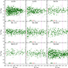 |
Fig. A.1. Projected phase-space diagrams of the nine clusters. The meaning of the symbols is the same as in Fig. 1. |
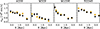 |
Fig. A.2. Line-of-sight velocity dispersion profiles of four clusters in our sample, based on our membership selection on mR magnitude cut samples (black dots) and on previous membership selections without magnitude cuts (gold squares) by Annunziatella et al. (2016), Girardi et al. (2024), Biviano et al. (2023), Sartoris et al. (2020) for A209, M329, M1206, and R2248, respectively. The error bars are 1σ. |
 |
Fig. A.3. VDPs of the nine clusters. The meaning of the symbols is the same as in Fig. 2. The MAMPOSSt solution for all clusters is that obtained for the gOM β(r) model, except for M1931 for which the gT model is used, since it gives a better fit than the gOM model. |
 |
Fig. A.4. 68% confidence regions for the MAMPOSStβsym(r) (blue) and for the JEIβsym(r) (red), for the nine clusters of our sample. The MAMPOSSt solution for all clusters is that obtained for the gOM β(r) model, except for M1931 for which the gT model is used, since it gives a better fit than the gOM model. The dashed horizontal line indicates isotropic orbits. Orbits are radial (respectively tangential) above (respectively below) this line. |
 |
Fig. A.5. Subclusters identified with the DS+ method in the nine clusters. Galaxies assigned to subclusters are shown as gray squares filled with different colors to distinguish the different subclusters. Cluster members outside subclusters are shown as black diamonds. No subcluster was identified in M329. The magenta dashed circle represents the r200 region, and the dotted lines identify the cluster center. |
All Tables
All Figures
|
Fig. 1. Projected phase-space diagram of the 427 galaxies selected as members of the M1206 cluster (other clusters are shown in Fig. A.1) by the CLUMPS method in the region R ≤ 1.36 r200. The three numbers at the bottom left indicate, from left to right, the number of galaxies selected for the dynamical analysis (black-circled green dots); the number of CLUMPS members that are excluded from the dynamical analysis because they are at R ≤ 0.05 Mpc, which is the region dynamically dominated by the BCG (red circles), and the number of CLUMPS members that are not used in the dynamical analysis because they are flagged as interlopers by the escape-velocity criterion (gray circles). The vertical lines indicate R = 0.05 Mpc and R = r200. The values of r200 and v200 come from U18. |
| In the text | |
|
Fig. 2. Dots with 1σ error bars: los VDP of M1206. Dashed blue line and cyan shading: Best-fit MAMPOSSt solution within 68% confidence levels, estimated on a random selection of 3000 MCMC steps. Red solid line and orange shading: JEI-predicted VDP and 68% confidence levels. The values of r200 (indicated by the vertical magenta line) and v200 are the best fits of the MAMPOSSt analysis (other clusters are shown in Fig. A.3.) |
| In the text | |
|
Fig. 3. Each panel shows the 1σ confidence levels of a cluster JEIβsym(r), as obtained from the procedure described in Sect. 3.3 (red shadings), and its central value (yellow line), the weighted mean of the nine profiles, ⟨βsym(r)⟩, as defined in Eq. (6) (black dash-dotted line), and the βsym(r) of the other eight clusters (black dotted lines). The horizontal dashed black line indicates isotropic orbits. Orbits are radial above this line and tangential below it. |
| In the text | |
|
Fig. 4. Results of the stepwise regression analysis (forward approach). Each square is the value of the coefficient of determination, R2, of dβ vs. the quantities labeled on the x-axis, with the inclusion of an additional quantity at each new point from left to right. |
| In the text | |
|
Fig. 5. dβ vs. M200. The symbol size is proportional to c200. The colors identify our nine clusters, in order of increasing redshift with increasing color wavelength (from blue to brown). |
| In the text | |
|
Fig. 6. Velocity anisotropy βsym at r = rvir, vs. velocity anisotropy at r = 0, for our nine clusters (colored dots) and for the lower-z clusters of Wojtak & Łokas (2010, black circles). The 1σ error bars are shown. The virial radius is rvir = r100 for the nearby clusters of Wojtak & Łokas (2010), and it is approximated by r126 for our clusters. The colors identify our nine clusters, in order of increasing redshift with increasing color wavelength (from blue to brown). |
| In the text | |
|
Fig. 7. β(r) of our nine clusters (colored solid lines) and of the ten nearby clusters of Li et al. (2023, black dot-dashed lines) displayed in the same format as that of Fig. 4 in Li et al. (2023). The colors identify our nine clusters, in order of increasing redshift with increasing color wavelength (from blue to brown). The vertical magenta dotted line indicates 1.5 r500, which is on average equivalent to r200 for our nine clusters. |
| In the text | |
|
Fig. 8. Upper panel: Nine clusters βsym(r) (color-coded in order of increasing redshift with increasing color wavelength, from blue to brown) and their weighted mean velocity anisotropy profile ⟨β(r)⟩ (dash-dotted black line) compared to the mean profile of 112 halos in the GAEA simulation (triple-dot-dashed gray line) and its rms (gray shading). Lower panel: Same as the upper panel, but the comparison is made with the mean profile of 25 halos in the RF simulation. |
| In the text | |
|
Fig. A.1. Projected phase-space diagrams of the nine clusters. The meaning of the symbols is the same as in Fig. 1. |
| In the text | |
|
Fig. A.2. Line-of-sight velocity dispersion profiles of four clusters in our sample, based on our membership selection on mR magnitude cut samples (black dots) and on previous membership selections without magnitude cuts (gold squares) by Annunziatella et al. (2016), Girardi et al. (2024), Biviano et al. (2023), Sartoris et al. (2020) for A209, M329, M1206, and R2248, respectively. The error bars are 1σ. |
| In the text | |
|
Fig. A.3. VDPs of the nine clusters. The meaning of the symbols is the same as in Fig. 2. The MAMPOSSt solution for all clusters is that obtained for the gOM β(r) model, except for M1931 for which the gT model is used, since it gives a better fit than the gOM model. |
| In the text | |
|
Fig. A.4. 68% confidence regions for the MAMPOSStβsym(r) (blue) and for the JEIβsym(r) (red), for the nine clusters of our sample. The MAMPOSSt solution for all clusters is that obtained for the gOM β(r) model, except for M1931 for which the gT model is used, since it gives a better fit than the gOM model. The dashed horizontal line indicates isotropic orbits. Orbits are radial (respectively tangential) above (respectively below) this line. |
| In the text | |
|
Fig. A.5. Subclusters identified with the DS+ method in the nine clusters. Galaxies assigned to subclusters are shown as gray squares filled with different colors to distinguish the different subclusters. Cluster members outside subclusters are shown as black diamonds. No subcluster was identified in M329. The magenta dashed circle represents the r200 region, and the dotted lines identify the cluster center. |
| In the text | |
Current usage metrics show cumulative count of Article Views (full-text article views including HTML views, PDF and ePub downloads, according to the available data) and Abstracts Views on Vision4Press platform.
Data correspond to usage on the plateform after 2015. The current usage metrics is available 48-96 hours after online publication and is updated daily on week days.
Initial download of the metrics may take a while.