| Issue |
A&A
Volume 708, April 2026
|
|
|---|---|---|
| Article Number | A345 | |
| Number of page(s) | 28 | |
| Section | Cosmology (including clusters of galaxies) | |
| DOI | https://doi.org/10.1051/0004-6361/202556310 | |
| Published online | 27 April 2026 | |
Euclid: Early Release Observations – Weak gravitational lensing analysis of Abell 2390 ★
1
Universität Innsbruck, Institut für Astro- und Teilchenphysik, Technikerstr. 25/8, 6020 Innsbruck, Austria
2
Universität Bonn, Argelander-Institut für Astronomie, Auf dem Hügel 71, 53121 Bonn, Germany
3
Institute for Astronomy, University of Edinburgh, Royal Observatory, Blackford Hill, Edinburgh EH9 3HJ, UK
4
Aix-Marseille Université, CNRS, CNES, LAM, Marseille, France
5
Institut d’Astrophysique de Paris, UMR 7095, CNRS, and Sorbonne Université, 98 bis boulevard Arago, 75014 Paris, France
6
Department of Astronomy, University of Geneva, ch. d’Ecogia 16, 1290 Versoix, Switzerland
7
Université Paris-Saclay, Université Paris Cité, CEA, CNRS, AIM, 91191 Gif-sur-Yvette, France
8
Instituto de Física de Cantabria, Edificio Juan Jordá, Avenida de los Castros, 39005 Santander, Spain
9
Leiden Observatory, Leiden University, Einsteinweg 55, 2333, CC, Leiden, The Netherlands
10
Universitäts-Sternwarte München, Fakultät für Physik, Ludwig-Maximilians-Universität München, Scheinerstrasse 1, 81679 München, Germany
11
Kobayashi-Maskawa Institute for the Origin of Particles and the Universe, Nagoya University, Chikusa-ku, Nagoya 464-8602, Japan
12
Institute for Advanced Research, Nagoya University, Chikusa-ku, Nagoya 464-8601, Japan
13
Kavli Institute for the Physics and Mathematics of the Universe (WPI), University of Tokyo, Kashiwa, Chiba 277-8583, Japan
14
Physics Program, Graduate School of Advanced Science and Engineering, Hiroshima University, 1-3-1 Kagamiyama, Higashi-Hiroshima, Hiroshima 739-8526, Japan
15
Hiroshima Astrophysical Science Center, Hiroshima University, 1-3-1 Kagamiyama, Higashi-Hiroshima, Hiroshima 739-8526, Japan
16
Core Research for Energetic Universe, Hiroshima University, 1-3-1, Kagamiyama, Higashi-Hiroshima, Hiroshima 739-8526, Japan
17
Department of Astronomy, University of Massachusetts, Amherst, MA 01003, USA
18
ESAC/ESA, Camino Bajo del Castillo, s/n., Urb. Villafranca del Castillo, 28692 Villanueva de la Cañada, Madrid, Spain
19
Institute of Space Sciences (ICE, CSIC), Campus UAB, Carrer de Can Magrans, s/n, 08193 Barcelona, Spain
20
Dipartimento di Fisica e Scienze della Terra, Università degli Studi di Ferrara, Via Giuseppe Saragat 1, 44122 Ferrara, Italy
21
INAF-Osservatorio di Astrofisica e Scienza dello Spazio di Bologna, Via Piero Gobetti 93/3, 40129 Bologna, Italy
22
Cosmic Dawn Center (DAWN)
23
Niels Bohr Institute, University of Copenhagen, Jagtvej 128, 2200 Copenhagen, Denmark
24
School of Mathematics and Physics, University of Surrey, Guildford, Surrey GU2 7XH, UK
25
Institut für Theoretische Physik, University of Heidelberg, Philosophenweg 16, 69120 Heidelberg, Germany
26
INAF-Osservatorio Astronomico di Brera, Via Brera 28, 20122 Milano, Italy
27
IFPU, Institute for Fundamental Physics of the Universe, via Beirut 2, 34151 Trieste, Italy
28
INAF-Osservatorio Astronomico di Trieste, Via G. B. Tiepolo 11, 34143 Trieste, Italy
29
INFN, Sezione di Trieste, Via Valerio 2, 34127 Trieste, TS, Italy
30
SISSA, International School for Advanced Studies, Via Bonomea 265, 34136 Trieste, TS, Italy
31
Dipartimento di Fisica e Astronomia, Università di Bologna, Via Gobetti 93/2, 40129 Bologna, Italy
32
INFN-Sezione di Bologna, Viale Berti Pichat 6/2, 40127 Bologna, Italy
33
INAF-Osservatorio Astronomico di Padova, Via dell’Osservatorio 5, 35122 Padova, Italy
34
Max Planck Institute for Extraterrestrial Physics, Giessenbachstr. 1, 85748 Garching, Germany
35
Dipartimento di Fisica, Università di Genova, Via Dodecaneso 33, 16146 Genova, Italy
36
INFN-Sezione di Genova, Via Dodecaneso 33, 16146 Genova, Italy
37
Department of Physics “E. Pancini”, University Federico II, Via Cinthia 6, 80126 Napoli, Italy
38
INAF-Osservatorio Astronomico di Capodimonte, Via Moiariello 16, 80131 Napoli, Italy
39
Instituto de Astrofísica e Ciências do Espaço, Universidade do Porto, CAUP, Rua das Estrelas, PT4150-762 Porto, Portugal
40
Faculdade de Ciências da Universidade do Porto, Rua do Campo de Alegre, 4150-007 Porto, Portugal
41
European Southern Observatory, Karl-Schwarzschild-Str. 2, 85748 Garching, Germany
42
Dipartimento di Fisica, Università degli Studi di Torino, Via P. Giuria 1, 10125 Torino, Italy
43
INFN-Sezione di Torino, Via P. Giuria 1, 10125 Torino, Italy
44
INAF-Osservatorio Astrofisico di Torino, Via Osservatorio 20, 10025 Pino Torinese (TO), Italy
45
European Space Agency/ESTEC, Keplerlaan 1, 2201, AZ, Noordwijk, The Netherlands
46
Institute Lorentz, Leiden University, Niels Bohrweg 2, 2333, CA, Leiden, The Netherlands
47
Mullard Space Science Laboratory, University College London, Holmbury St Mary, Dorking, Surrey RH5 6NT, UK
48
INAF-IASF Milano, Via Alfonso Corti 12, 20133 Milano, Italy
49
INAF-Osservatorio Astronomico di Roma, Via Frascati 33, 00078 Monteporzio Catone, Italy
50
INFN-Sezione di Roma, Piazzale Aldo Moro, 2 – c/o Dipartimento di Fisica, Edificio G. Marconi, 00185 Roma, Italy
51
Centro de Investigaciones Energéticas, Medioambientales y Tecnológicas (CIEMAT), Avenida Complutense 40, 28040 Madrid, Spain
52
Port d’Informació Científica, Campus UAB, C. Albareda s/n, 08193 Bellaterra (Barcelona), Spain
53
Institute for Theoretical Particle Physics and Cosmology (TTK), RWTH Aachen University, 52056 Aachen, Germany
54
Institut d’Estudis Espacials de Catalunya (IEEC), Edifici RDIT, Campus UPC, 08860 Castelldefels, Barcelona, Spain
55
INFN section of Naples, Via Cinthia 6, 80126 Napoli, Italy
56
Institute for Astronomy, University of Hawaii, 2680 Woodlawn Drive, Honolulu, HI 96822, USA
57
Dipartimento di Fisica e Astronomia “Augusto Righi” – Alma Mater Studiorum Università di Bologna, Viale Berti Pichat 6/2, 40127 Bologna, Italy
58
Instituto de Astrofísica de Canarias, Vía Láctea, 38205 La Laguna, Tenerife, Spain
59
Jodrell Bank Centre for Astrophysics, Department of Physics and Astronomy, University of Manchester, Oxford Road, Manchester M13 9PL, UK
60
European Space Agency/ESRIN, Largo Galileo Galilei 1, 00044 Frascati, Roma, Italy
61
Université Claude Bernard Lyon 1, CNRS/IN2P3, IP2I Lyon, UMR 5822, Villeurbanne F-69100, France
62
Institut de Ciències del Cosmos (ICCUB), Universitat de Barcelona (IEEC-UB), Martí i Franquès 1, 08028 Barcelona, Spain
63
Institució Catalana de Recerca i Estudis Avançats (ICREA), Passeig de Lluís Companys 23, 08010 Barcelona, Spain
64
UCB Lyon 1, CNRS/IN2P3, IUF, IP2I Lyon, 4 rue Enrico Fermi, 69622 Villeurbanne, France
65
Departamento de Física, Faculdade de Ciências, Universidade de Lisboa, Edifício C8, Campo Grande, PT1749-016 Lisboa, Portugal
66
Instituto de Astrofísica e Ciências do Espaço, Faculdade de Ciências, Universidade de Lisboa, Campo Grande, 1749-016, Lisboa, Portugal
67
Université Paris-Saclay, CNRS, Institut d’astrophysique spatiale, 91405 Orsay, France
68
INFN-Padova, Via Marzolo 8, 35131 Padova, Italy
69
Aix-Marseille Université, CNRS/IN2P3, CPPM, Marseille, France
70
INAF-Istituto di Astrofisica e Planetologia Spaziali, via del Fosso del Cavaliere, 100, 00100, Roma, Italy
71
Space Science Data Center, Italian Space Agency, via del Politecnico snc, 00133, Roma, Italy
72
INFN-Bologna, Via Irnerio 46, 40126 Bologna, Italy
73
Institute of Theoretical Astrophysics, University of Oslo, P.O. Box 1029 Blindern 0315, Oslo, Norway
74
Jet Propulsion Laboratory, California Institute of Technology, 4800 Oak Grove Drive, Pasadena, CA 91109, USA
75
Department of Physics, Lancaster University, Lancaster LA1 4YB, UK
76
Felix Hormuth Engineering, Goethestr. 17, 69181 Leimen, Germany
77
Technical University of Denmark, Elektrovej 327, 2800 Kgs., Lyngby, Denmark
78
Cosmic Dawn Center (DAWN), Denmark
79
Max-Planck-Institut für Astronomie, Königstuhl 17, 69117 Heidelberg, Germany
80
NASA Goddard Space Flight Center, Greenbelt, MD 20771, USA
81
Department of Physics and Astronomy, University College London, Gower Street, London WC1E 6BT, UK
82
Department of Physics and Helsinki Institute of Physics, Gustaf Hällströmin katu 2, 00014 University of Helsinki, Finland
83
Université de Genève, Département de Physique Théorique and Centre for Astroparticle Physics, 24 quai Ernest-Ansermet, CH-1211 Genève 4, Switzerland
84
Department of Physics, P.O. Box 64, 00014 University of Helsinki, Finland
85
Helsinki Institute of Physics, Gustaf Hällströmin katu 2 University of Helsinki, Helsinki, Finland
86
Kapteyn Astronomical Institute, University of Groningen, PO Box 800, 9700 AV, Groningen, The Netherlands
87
Laboratoire d’etude de l’Univers et des phenomenes eXtremes, Observatoire de Paris, Université PSL, Sorbonne Université, CNRS, 92190 Meudon, France
88
SKA Observatory, Jodrell Bank, Lower Withington, Macclesfield, Cheshire SK11 9FT, UK
89
Centre de Calcul de l’IN2P3/CNRS, 21 avenue Pierre de Coubertin, 69627 Villeurbanne Cedex, France
90
Dipartimento di Fisica “Aldo Pontremoli”, Università degli Studi di Milano, Via Celoria 16, 20133 Milano, Italy
91
INFN-Sezione di Milano, Via Celoria 16, 20133 Milano, Italy
92
University of Applied Sciences sand Arts of Northwestern Switzerland, School of Computer Science, 5210 Windisch, Switzerland
93
Dipartimento di Fisica e Astronomia “Augusto Righi” – Alma Mater Studiorum Università di Bologna, via Piero Gobetti 93/2, 40129 Bologna, Italy
94
Department of Physics, Institute for Computational Cosmology, Durham University, South Road, Durham DH1 3LE, UK
95
Université Côte d’Azur, Observatoire de la Côte d’Azur, CNRS, Laboratoire Lagrange, Bd de l’Observatoire, CS 34229, 06304 Nice cedex 4, France
96
Université Paris Cité, CNRS, Astroparticule et Cosmologie, 75013 Paris, France
97
CNRS-UCB International Research Laboratory, Centre Pierre Binétruy, IRL2007, CPB-IN2P3, Berkeley, USA
98
Institut d’Astrophysique de Paris, 98bis Boulevard Arago, 75014 Paris, France
99
Institute of Physics, Laboratory of Astrophysics, Ecole Polytechnique Fédérale de Lausanne (EPFL), Observatoire de Sauverny, 1290 Versoix, Switzerland
100
University Observatory, LMU Faculty of Physics, Scheinerstrasse 1, 81679 Munich, Germany
101
Telespazio UK S.L. for European Space Agency (ESA), Camino bajo del Castillo, s/n, Urbanizacion Villafranca del Castillo, Villanueva de la Cañada, 28692, Madrid, Spain
102
Institut de Física d’Altes Energies (IFAE), The Barcelona Institute of Science and Technology, Campus UAB, 08193 Bellaterra (Barcelona), Spain
103
DARK, Niels Bohr Institute, University of Copenhagen, Jagtvej 155, 2200 Copenhagen, Denmark
104
Waterloo Centre for Astrophysics, University of Waterloo, Waterloo, Ontario N2L 3G1, Canada
105
Department of Physics and Astronomy, University of Waterloo, Waterloo, Ontario N2L 3G1, Canada
106
Perimeter Institute for Theoretical Physics, Waterloo, Ontario N2L 2Y5, Canada
107
Centre National d’Etudes Spatiales – Centre spatial de Toulouse, 18 avenue Edouard Belin, 31401 Toulouse Cedex 9, France
108
Institute of Space Science, Str. Atomistilor, nr. 409 Măgurele, Ilfov 077125, Romania
109
Dipartimento di Fisica e Astronomia “G. Galilei”, Università di Padova, Via Marzolo 8, 35131 Padova, Italy
110
Institut de Recherche en Astrophysique et Planétologie (IRAP), Université de Toulouse, CNRS, UPS, CNES, 14 Av. Edouard Belin, 31400 Toulouse, France
111
Université St Joseph; Faculty of Sciences, Beirut, Lebanon
112
Departamento de Física, FCFM, Universidad de Chile, Blanco Encalada 2008, Santiago, Chile
113
Satlantis, University Science Park, Sede Bld 48940 Leioa-Bilbao, Spain
114
Department of Physics, Royal Holloway, University of London, TW20 0EX, UK
115
Instituto de Astrofísica e Ciências do Espaço, Faculdade de Ciências, Universidade de Lisboa, Tapada da Ajuda, 1349-018 Lisboa, Portugal
116
Universidad Politécnica de Cartagena, Departamento de Electrónica y Tecnología de Computadoras, Plaza del Hospital 1, 30202 Cartagena, Spain
117
Infrared Processing and Analysis Center, California Institute of Technology, Pasadena, CA 91125, USA
118
INAF, Istituto di Radioastronomia, Via Piero Gobetti 101, 40129 Bologna, Italy
119
Department of Physics, Oxford University, Keble Road, Oxford OX1 3RH, UK
120
Aurora Technology for European Space Agency (ESA), Camino bajo del Castillo, s/n, Urbanizacion Villafranca del Castillo, Villanueva de la Cañada, 28692, Madrid, Spain
121
INAF – Osservatorio Astronomico di Brera, via Emilio Bianchi 46, 23807 Merate, Italy
122
ICL, Junia, Université Catholique de Lille, LITL, 59000 Lille, France
123
ICSC – Centro Nazionale di Ricerca in High Performance Computing, Big Data e Quantum Computing, Via Magnanelli 2, Bologna, Italy
124
Department of Physics and Astronomy, University of British Columbia, Vancouver, BC V6T 1Z1, Canada
★★ Corresponding author: This email address is being protected from spambots. You need JavaScript enabled to view it.
Received:
8
July
2025
Accepted:
6
January
2026
Abstract
The Euclid space telescope of the European Space Agency (ESA) is designed to provide sensitive and accurate measurements of weak gravitational lensing distortions over wide areas on the sky. Here, we present a weak gravitational lensing analysis of early Euclid observations obtained for the field around the massive galaxy cluster Abell 2390 as part of the Euclid Early Release Observations (ERO) programme. We conducted shape measurements for galaxies down to IE ≲ 26.5 using three independent algorithms (LensMC, KSB+, and SourceXtractor++). Incorporating multi-band photometry from Euclid and Subaru/Suprime-Cam, we estimated photometric redshifts to preferentially select background sources from tomographic redshift bins, for which we calibrated the redshift distributions using the self-organising map approach and data from the Cosmic Evolution Survey (COSMOS). We quantified the residual cluster member contamination and corrected for it in bins of photometric redshift and magnitude using their source density profiles, including corrections for source obscuration and magnification. We reconstructed the cluster mass distribution and jointly fit the tangential reduced shear profiles of the different tomographic bins with spherical Navarro-Frenk-White profile predictions to constrain the cluster mass, finding consistent results for the three shape catalogues and good agreement with earlier measurements. As an important validation test, we compared these joint constraints to mass measurements obtained individually for the different tomographic bins, finding a good level of consistency. More detailed constraints on the cluster properties are presented in a companion paper, which additionally incorporates strong lensing measurements. Our analysis provides a first demonstration of the outstanding capabilities of Euclid for tomographic weak lensing measurements.
Key words: gravitational lensing: weak / galaxies: clusters: general / galaxies: clusters: individual: Abell 2390 / dark matter
This paper is published on behalf of the Euclid Consortium.
© The Authors 2026
 Open Access article, published by EDP Sciences, under the terms of the Creative Commons Attribution License (https://creativecommons.org/licenses/by/4.0), which permits unrestricted use, distribution, and reproduction in any medium, provided the original work is properly cited.
This article is published in open access under the Subscribe to Open model. This email address is being protected from spambots. You need JavaScript enabled to view it. to support open access publication.
1. Introduction
The primary objective of the European Space Agency’s new space telescope Euclid is to test cosmological models using measurements of galaxy clustering and weak gravitational lensing (Euclid Collaboration: Mellier 2025). For this purpose, Euclid will observe approximately 14 000 deg2 of the extragalactic sky in the Euclid Wide Survey (EWS, Euclid Collaboration: Scaramella 2022) using its visual charge-coupled device (CCD) imager VIS (Euclid Collaboration: Cropper 2025) and its near-infrared instrument NISP (Euclid Collaboration: Jahnke 2025). With their fine pixel sampling (0 1 pixel scale) and space-based resolution, the VIS images will be used to measure the shapes of approximately 1.5 billion galaxies in order to constrain weak lensing (WL) distortions caused by the gravitational potential of foreground structures (for an introduction to WL, see e.g. Bartelmann & Schneider 2001). Typically these distortions are weak and change the axis ratios of galaxy images at the per cent level only. In this regime, which is typically referred to as ‘cosmic shear’, cosmological parameters are inferred by measuring correlations in galaxy ellipticities as a function of their separation, averaged over large sky areas (e.g. Hamana et al. 2020; Amon et al. 2022; Asgari et al. 2021). However, WL data can also result in competitive cosmological constraints (see e.g. Mantz et al. 2015; Bocquet et al. 2019, 2024b; Ghirardini et al. 2024) when they are used to calibrate the mass scale (e.g. Schrabback et al. 2021; Zohren et al. 2022; Chiu et al. 2022; Grandis et al. 2024; Kleinebreil et al. 2025) of galaxy cluster samples that are characterised by a cosmologically well modelled selection function (e.g. Bleem et al. 2015, 2020, 2024; Hilton et al. 2021; Bulbul et al. 2024; Aymerich et al. 2024). In such cases, WL data break degeneracies that exist between parameters describing the cosmological model on the one hand and cluster mass-observable scaling relations on the other (e.g. Grandis et al. 2019; Bocquet et al. 2024a).
Massive galaxy clusters create WL distortions that are strong enough to be detected for a single target if deep high-resolution imaging is employed, providing a high density of background galaxies with WL shape measurements (e.g. von der Linden et al. 2014a,b; Hoekstra et al. 2015; Sereno et al. 2017; Herbonnet et al. 2020; Kim et al. 2021). Such observations were performed by Euclid for the extremely massive galaxy cluster Abell 2390 (A2390 hereafter; see Abell et al. 1989), located at redshift z = 0.228 (Sohn et al. 2020), as part of the Euclid Early Release Observations (ERO, 2024) ‘Magnifying Lens’ programme (Atek et al. 2025). These observations provide an excellent opportunity to showcase Euclid’s outstanding capability to measure the WL signature of a massive galaxy cluster, which is the main goal of this paper. Simultaneously, this paper demonstrates some analysis approaches for tomographic Euclid cluster WL studies that can be employed in future investigations of larger samples.
Initial WL constraints based the Euclid observations of A2390 were reported in the wider overview paper by Atek et al. (2025). We have significantly improved upon this analysis by incorporating two additional shape measurement methods, a source selection via tomographic redshift bins, improved calibrations, and a correction for cluster member contamination. Other earlier WL studies of this cluster were limited to ground-based observations, including an early work by Squires et al. (1996), as well as the ‘Weighing the Giants’ project (WtG, von der Linden et al. 2014a; Applegate et al. 2014), the Local Cluster Substructure Survey (LoCuSS, Okabe & Smith 2016), the Canadian Cluster Comparison Project (CCCP, Hoekstra et al. 2015; Herbonnet et al. 2020), and the recent analysis of WIYN-ODI data by Dutta et al. (2024). Of these, WtG and LoCuSS employed ground-based observations from Subaru/Suprime-Cam, which we incorporated into our analysis for the photometric source selection (see Sect. 2.2).
This paper is organised as follows. In Sect. 2, we describe the data used in our study, including the Euclid observations and complementary archival ground-based data. In Sect. 3, we detail the computation of photometric redshifts and their calibration. Section 4 summarises our measurements of WL galaxy shapes, where we employ and compare three different shape measurement algorithms. We quantify and account for cluster member contamination in Sect. 5, followed by the presentation of the WL mass constraints and reconstruction in Sect. 6. We discuss our results and compare them to previous WL measurements of the cluster in Sect. 7, followed by our conclusions in Sect. 8.
Throughout our analysis, we assumed a standard flat ΛCDM cosmology characterised via parameters ΩΛ = 0.7, Ωm = 0.3, and H0 = 70 km s−1 Mpc−1. For the computation of WL noise caused by large-scale structure projections (see Sect. 6.3.2), we additionally assumed σ8 = 0.8, Ωb = 0.046, and ns = 0.96. All magnitudes given in this paper are in the AB system.
2. Data
2.1. Euclid observations
Euclid’s A2390 observations were obtained on 28 November 2023 during Euclid’s performance verification (PV) phase as part of the ERO programme (Cuillandre et al. 2025). They consist of three dithered Euclid Reference Observing Sequences (ROS; see Euclid Collaboration: Scaramella 2022; Euclid Collaboration: Mellier 2025) of 70.2 min each. To fill detector gaps each ROS contains four dither positions. At each dither position, a 566 s exposure was taken with VIS in its broad optical band-pass (approximately 540–920 nm, referred to as IE; see Euclid Collaboration: Cropper 2025), while a 574 s spectroscopic exposure was simultaneously obtained with NISP. These were followed by NISP images in the YE, JE, and HE filters (Euclid Collaboration: Jahnke 2025), each with an exposure time of 112 s. For the ERO observations, an additional short (95 s) VIS exposure was taken during each YE exposure, leading to a total integration time of 7932 s for A2390 with VIS.
As detailed in Cuillandre et al. (2025), stacks were created for each filter using the ERO reduction pipeline and the AstrOmatic SWarp software (Bertin et al. 2002) at the native pixel scales of the corresponding instruments (0 1 for VIS and 0
 3 for NISP). In particular, there are two flavours of stacks, where the ‘flattened’ version employs a 64 pixel mesh and 3× smoothing factor to model and subtract the background (Cuillandre et al. 2025). This approach is optimised for the photometry of faint and compact objects and therefore employed for the computation of multi-band photometry (see Sect. 2.4). An alternative set of stacks is optimised for the analysis of low surface brightness (LSB) sources (‘LSB’ version) and therefore does not apply a background subtraction. For initial tests we conducted WL shape measurements (see Sect. 4) on both versions of the stacks. Given that we found only minimal differences, we conducted the main analysis using the ‘flattened’ version to remain consistent with the photometric analysis. Further details on the A2390 ERO data are provided in Atek et al. (2025), including estimates of the 5σ limiting magnitudes of the stacked images, which amount to IE = 27.01 for the VIS stack (assuming apertures with diameter 0
 3) and YE = 25.18, JE = 25.22, and HE = 25.12 for the NISP stacks (all assuming apertures with diameter 0
 6).
6).
2.2. Earlier ground-based observations
Archival ground-based multi-band imaging data are available for the A2390 field thanks to earlier programmes studying the WL signature of the cluster (see Sect. 1). While we expect the Euclid VIS images to be superior for the measurement of galaxy shapes, given their outstanding resolution, the inclusion of multi-band ground-based data is still important for the photometric selection of background sources. For this purpose, we incorporated existing (B, V, Rc, i, Ic, z′) imaging obtained with the Suprime-Cam instrument on the 8.2 m Subaru telescope (Miyazaki et al. 2002) and also considered Canada-France-Hawaii Telescope (CFHT) Megacam u-band imaging taken with the first generation MP9301 u-filter. These data were previously employed by the WtG project (von der Linden et al. 2014a) and in part by the LoCuSS project (Okabe & Smith 2016).
In our analysis, we made use of a custom reduction of the Suprime-Cam data using the SDFRED pipeline (Yagi et al. 2002; Ouchi et al. 2004), processed at the Suprime-Cam Legacy Archive at the Canadian Astronomy Data Centre (Gwyn 2020). Likewise, CFHT Megacam u-band images were reduced with the Elixir pipeline1 (Magnier 2002; Magnier & Cuillandre 2004). All these frames were jointly astrometrically registered using scamp (Bertin et al. 2002) and Gaia-DR3 as a reference sample, yielding a typical 10–20 mas absolute astrometric accuracy in right ascension (RA) and declination (Dec). We created models of the spatially varying point spread function (PSF) for all of the ground-based data bands using PSFEx (Bertin 2011), facilitating PSF photometry on all stars that properly accounts for seeing variations and eases photometric calibration. This calibration was performed on individual frames using photometric reference catalogues from the Sloan Digital Sky Survey (Ahumada et al. 2020) for the u band and from the Pan-STARRS 3π survey (Chambers et al. 2016) for all Suprime-Cam bands. The colour terms are more uncertain for the Johnson B, V and Cousins Rc, Ic filters compared to the Sloan i and z bands, but overall a very uniform photometric calibration is reached (Gwyn 2020). Prior to the exposure stacking, we used the MaxiMask (Paillassa et al. 2020) tool to flag cosmic rays, hot pixels, satellite trails, bad columns, saturation bleeds near bright stars, and other defects. Taking those flags into account in the weighting scheme, exposures were then stacked using swarp (Bertin et al. 2002) on a  pixel scale, common to all ground-based filters. At this stage, no attempt to correct for Galactic extinctions was made.
Most of the 28′×34′ area covered by the Suprime-Cam images overlaps with the full-depth area of the Euclid VIS stack (see Fig. 1). We regard this overlap area, which is also fully encompassed by the Megacam u-band image, as the primary region of interest for our WL study. This is both due to the full multi-wavelength coverage and the fact that this area already provides complete azimuthal coverage out to a projected radius of 3.07 Mpc from the cluster centre (at the reference cosmology), well beyond the expected virial radius of the cluster. In contrast, measurements at significantly larger radii would probe the WL signal in the regime of the two-halo term, which is more difficult to model accurately and, therefore, they are typically excluded in cluster scaling relation and cosmology analyses (e.g. Dietrich et al. 2019; Grandis et al. 2021).
 |
Fig. 1. Field coverage. The grey-scale shows the weight image of the VIS image stack on a linear scale. The magenta solid polygon indicates the main region of interest for this WL analysis, where both the Euclid image stacks have their greatest depth and multi-band ground-based observations are available. The cyan dashed polygon indicates the full-depth VIS area employed in the source injection analysis (see Sect. 5.2). |
2.3. Removal of foreground Galactic cirrus
A2390 resides at relatively low Galactic latitude ( ), leading to prominent foreground emission due to dust cirrus. Ellien et al. (2025) used the same Euclid ERO data to investigate the low-surface-brightness intra-cluster light distribution of A2390 and describe the properties of the cirrus emission in more detail. In the present work, we wish to ensure minimal impact of the cirrus emission on the WL analysis and subtract it via an advanced background model.
This can be achieved using the DeNeb tool, a new deep-learning software package designed to perform single-channel source separation on astronomical images (Bertin et al., in prep.). DeNeb was trained on a large gallery of labelled images from various origins to perform the subtraction of extended features comprised of reflection haloes from bright stars, residual flat-fielding and fringing patterns, and diffuse emission and reflection from Galactic dust, while preserving stellar and galaxy images.
All the stacks, either Euclid or ground-based, were independently processed with the default DeNeb tool. Due to the lack of network training with u-band data, the method resulted in a slightly poorer removal of diffuse extended components in that filter, with an occasional removal of parts of very extended foreground galaxies. These are, however, irrelevant for our scientific goals. On the contrary, for all other filters, the subtraction was very effective. For the remainder of the analysis we will work exclusively with ‘denebulised’ images. These provide the major advantage of a much flatter background, which leads to a more robust object detection and deblending.
Notably, the patchy foreground emission caused by the scattering of starlight off Galactic dust also comes with equally complex extinction variations. These have not been corrected via the procedure described here and remain a possible concern for photometric redshift estimation (see Sect. 3).
2.4. Object detection and SourceXtractor++ measurements
Here, we employed the photometric catalogue first presented in Atek et al. (2025). This catalogue was generated using SourceXtractor++ (Bertin et al. 2022; Kümmel et al. 2022, henceforth SE++), a recent re-implementation of SExtractor (Bertin & Arnouts 1996). We ran SE++ in two settings, but source detection was always performed in the VIS IE band. In the first run, only the VIS image was used to constrain a single Sérsic profile. This provides shapes that can readily be used for WL, and best-fit sizes provide a complementary star-and-galaxy discriminator, since the best effective radius for unsaturated stars is consistently small. The WL exploitation of the single Sérsic models is further described in Sect. 4.3.
For the photometric catalogue, objects are detected on the VIS IE stack, followed by a joint fit of the Euclid and ground-based images using a two-component galaxy model with a de Vaucouleurs-profile bulge and an exponential disc. This fit assumed identical bulge and disc orientations, but allowed for free axis ratios. Furthermore, the half-light radii of the bulge and disc were modelled to be wavelength independent, with varying bulge-to-total flux ratios between bands.
With version 0.19, our analysis employs the latest version of SE++ available at the time of the data processing. It groups neighbouring sources in order to jointly fit their surface brightness profiles, which reduces the impact of blending compared to traditional approaches such as PSF-homogenised aperture photometry. Since the processing of these ERO data, the development of SE++ has continued, leading to further improvements that will be implemented for the analysis of future Euclid datasets. In particular, a full operational decoupling of the detection and model-fitting steps is expected to improve the performance in the case of objects that are fully separated in VIS, but still partially blended in the ground-based data. However, for our analysis we expect this to be a minor issue, given the superb image quality of the ground-based data (Atek et al. 2025). Furthermore, in the computation of photometric redshifts optical colours are only incorporated based on ground-based instruments (see Sect. 3), which further reduces the potential impact of any mismatches between the ground- and space-based data for the photometry.
More details about the SE++ runs, including overall photometric accuracy and star/galaxy separation with single Sérsic fits can be found in Appendix A. All such runs rely on a common model of the Euclid PSF, which is described in the next subsection.
2.5. Point-spread function modelling
In the context of these ERO observations, PSF models of the different image stacks were obtained using PSFEx (Bertin 2011), while a more advanced model of the Euclid VIS PSF is being developed for future WL analyses of larger samples (see section 7.6.4. in Euclid Collaboration: Mellier 2025). To limit the potential impact of brighter-fatter effects (see e.g. Guyonnet et al. 2015), we halved the PSFEx input values for detector saturation compared to their actual values. With this precaution, only stars with a photometric signal-to-noise ratio2 of 70 ≤ S/Nflux ≲ 1500 were retained to build the model. This is most relevant for VIS, which provides most of the morphological information. An image of the rendered VIS PSF is shown in Fig. 2. The mean PSF full width at half maximum (FWHM) is  , while average PSF ellipticities (ϵ1PSFEx, ϵ2PSFEx) amount to (−0.0152, 0.0017) in the stacked image pixel frame. PSFEx models were rendered with a finer pixel scale of
  ,
,  , and
, and  for VIS, NISP, and ground-based images, respectively, assuming a third-order polynomial to capture spatial variations across the whole focal plane. We did not attempt to model the wavelength dependence of the VIS PSF for this single-target study, given its moderate accuracy requirements. In the case of the VIS PSF, our model extends to
  and only misses 3% of the encircled energy when compared to Table 3 of Cuillandre et al. (2025). Given that SE++ normalises the PSF convolution kernel to unity, this should be taken into account when employing computed model magnitudes of point sources. In the case of NISP bands, the PSF model extends to
  and encloses between 98% and 98.5% of the total energy. Modest additional corrections, taking into account the energy enclosed in very extended diffraction spikes, should be considered for stellar photometry (Cuillandre et al. 2025). In the case of ground-based data, our PSF models extend to a
  radius for all filters. Given the exquisite seeing conditions (
 FWHM) of the employed ground-based data (Atek et al. 2025), corrections are negligible for stellar photometry in those ground-based filters.
 |
Fig. 2. VIS PSF recovered by PSFEx in the centre of the field of view. Pixel intensities are scaled on a logarithmic stretch. The image sampling is |

2.6. Masking
Atek et al. (2025) described the semi-automated generation of masks for the field, aiming to exclude spurious detections and light contamination near the haloes or diffraction spikes of stars, as well as stellar ghost images. We apply these masks to all of our catalogues and furthermore exclude regions affected by very extended low-redshift galaxies, whose sub-structure (e.g. extended spiral arms) might otherwise be incorrectly deblended into smaller objects.
3. Photometric redshifts
The computation of photometric redshifts (photo-zs) and the calibration of their redshift distributions is conducted in two steps and broadly follows the pattern established for Euclid WL cosmology analyses (Masters et al. 2015; Euclid Collaboration: Mellier 2025), as well as precursor Stage-III WL surveys (e.g. Hildebrandt et al. 2021; Myles et al. 2021). Firstly, galaxies are assigned to sub-samples on the basis of their best-estimated photometric redshift. Secondly, the redshift distribution within each of these tomographic redshift bins is inferred by matching the target galaxies to a reference dataset in their high-dimensional photometric space. The following subsections detail these two steps.
3.1. Photo-z point estimates
We computed photometric redshifts for galaxies in the Euclid and Subaru overlap area using the Phosphoros3 package (Paltani et al., in prep.), developed for the Euclid Science Ground Segment. Phosphoros is a fully Bayesian template-fitting code that shares many of the features of LePhare (Arnouts et al. 1999; Ilbert et al. 2006), on which it was initially modelled, but expands upon the functionality and flexibility of its predecessor (see the documentation and Paltani et al., in prep., for details).
Template-fitting approaches to photo-z estimation are susceptible to biases and spurious peaks in redshift in the presence of systematic uncertainties, especially in the form of unknown zero-point calibration offsets, photometric measurement biases, template mis-specification, and errors in the passband throughput curves. Disentangling, measuring, and correcting for these various effects is at best a laborious task, and in most cases simply intractable. A pragmatic alternative that is often employed (e.g. Weaver et al. 2022) is to use the sub-set of the data with known redshifts to identify systematic differences between the predicted fluxes from their best-matching templates (at fixed redshift) and their measured values; then to apply calibration offsets to the data. In this approach, errors in the templates (for example) get absorbed into the photometric calibration, improving the measured redshifts for objects represented by the spectroscopic sub-set, but leaving unknown biases for those that are not. Nevertheless, some confidence can be gained by examining the photometric offsets as a function of redshift (e.g. Hartley et al. 2022). Errors in the templates and filter curves introduce redshift-varying offsets, while true calibration errors produce constant offsets. To guard against residual biases (especially in galaxies that are not represented among the spectroscopic objects), a systematic uncertainty of between a few to ten per cent of an object’s flux is typically added in quadrature to the measured flux uncertainties in each band.
In the case of our A2390 data we have very limited spectroscopic information, consisting mostly of cluster member galaxies, and the additional complication of moderately high Galactic reddening. In particular, the reddening can be problematic in the case of structure on scales finer than the Planck map (Planck Collaboration XI 2014) we use when applying attenuation to the templates. Indeed, the cirrus emission that we subtracted (see Sect. 2.3) varies on very fine spatial scales and we found we were unable to obtain a stable value for the CFHT u-band photometric adjustment. As a result, we dropped this band from our current work. We also dropped the IE band during photo-z measurement, on account of the lack of chromatic corrections in the current version of our catalogues. As outlined in Cuillandre et al. (2025), the very broad passband of IE makes low-level detrending operations (e.g. flat-fielding) chromatic in nature, and thus require corrections to measured object photometry at a later stage. At this time, those necessary corrections are not in place for the ERO data and so, we would expect to see significant colour-dependent biases in the photometric measurements of galaxies. Such biases have been confirmed by visual inspection of their multi-band spectral energy distributions (SEDs), with the IE band often low with respect to the other red optical bands. Since we have access to deep multi-band photometry from Subaru Suprime-Cam for the purposes of this work, we were able to proceed without the IE photometric information for the computation of photo-z values. We will address the necessary corrections in the future.
With the three NISP bands and six Suprime-Cam bands, we proceeded to the photometric zero-point adjustment. We gathered the spectroscopic redshifts via CDS4, combining datasets from Lamareille et al. (2006), Nakamura et al. (2006), Rines et al. (2018), and Sohn et al. (2020), with most objects contained in the Sohn et al. (2020) compilation. In total, we acquired 330 spectroscopic redshifts (after excluding known active galactic nuclei), of which about 80% are at or close to the cluster redshift. The Phosphoros set-up we used for the systematic photometric adjustments and to measure photo-z point estimates and probability distributions for the whole catalogue is summarised in Table 1. The photometric adjustment factors that we derive through this process are listed in Table 2, alongside the systematic fractional flux uncertainties that we applied during the photo-z measurement run.
Configuration parameters for the Phosphoros photo-z package.
Photometric magnitude zero-point adjustments (i.e. a relative factor applied to the source fluxes) and fractional systematic flux uncertainties applied during photometric redshift computation.
Phosphoros outputs both the redshift corresponding to the maximum of the multi-dimensional posterior distribution and the marginalised maximum posterior redshift. To construct our tomographic redshift sub-samples we use the peak of the 1D marginalised redshift distribution because it performs marginally better on the spectroscopic set of objects than the other point estimates we measure. Figure 3 shows the comparison of our measured photo-z with the spectroscopic redshifts. The outlier rate, η = 3%, is defined as the fraction of sources with scaled residuals Δz = (zspec − zphot)/(1 + zspec) exceeding 0.15 in absolute value, while the normalised median absolute deviation, NMAD = 0.03, is defined as the normalised median absolute deviation of the residuals, NMAD = 1.4826 × median(|Δz − median(Δz)|). Both values are typical for a sample of reasonably bright galaxies with deep optical to near-infrared broadband photometry. Although the spectroscopic sample is small, these numbers are encouraging given the manipulations to the images that were required to remove the cirrus emission.
 |
Fig. 3. Comparison of the Phosphoros-derived photometric redshifts zph, where the points show the photometric redshift estimate defined as the peak of the 1D marginalised redshift distribution, while the error bars indicate the 16–84 percentiles of the probability distribution function, with spectroscopic redshifts (zsp) for sources in the A2390 field. The top panel shows the direct comparison, while the bottom panel displays the redshift residuals defined as (zsp − zph)/(1 + zsp). The normalised median absolute deviation (NMAD) and outlier rate (η) are indicated. Dashed lines at ±0.15 show the residual threshold. |
The boundaries of our redshift bins are pre-defined, taking into account the expected overall distribution of objects in redshift, the desire to avoid (as far as possible) cluster member galaxies, and the dependence of photo-z precision on the overall S/Nflux of the photometry. We define two magnitude ranges, 22 < IE < 24.5 (bright sample) and 24.5 < IE < 26.5 (faint sample), with the intention of producing reasonably tight and well-separated bins for objects with more precise photo-z (brighter objects), and broader bins for fainter, more difficult to measure objects that are more numerous at higher redshifts. We form six bins in redshift, four of which are used in the cluster mass measurement (avoiding the cluster itself and galaxies at very high redshifts, where template degeneracies are known to have an impact). See Table 3 for the number of objects in the different combinations of magnitude and photometric redshift bins.
Number of objects in different magnitude and photometric redshift bins.
3.2. Construction of the redshift distributions
Building accurate redshift distributions, n(z), for samples of galaxies is a topic that has received a great deal of attention in the WL literature over recent years. The role that the mean redshift (in particular) plays in the cosmological interpretation of a measured WL signal has placed redshift measurements at the centre of studies of systematic uncertainties (see Newman & Gruen 2022, for a review). A broad consensus has emerged around two main methods for redshift inference: (i) cross-correlation with a finely redshift-binned tracer sample (Newman 2008) and (ii) matching the target galaxies in colour space to a known reference set of objects (Lima et al. 2008; Masters et al. 2015). Since cross-correlation typically requires large sky areas to build sufficient constraining power, we chose to employ only the colour space matching method.
The tool used by most recent cosmological analyses for calibrating the relation between redshift and the photometric space of a particular survey is a self-organising map (SOM), introduced by Masters et al. (2015) for the purpose of meeting the extremely tight redshift requirements in Euclid. An SOM is an unsupervised machine-learning method for dimensionality reduction that produces a 2D array of nodes (or ‘cells’) from the higher dimensional space, while preserving locality. Specifically, neighbouring points in the high-dimensional space remain neighbours in the non-linear projection to two dimensions. Its value for redshift calibration is that the cells provide a partitioning of the photometric space that depends on the nature of the data itself. In other words, heavily occupied regions of colour space get split more finely (allowing for greater redshift fidelity), spurious objects tend to collect into small noticeable regions of the map and can be excluded, and troublesome cells, where degeneracies in redshift may occur, can also be predicted. However, most importantly, this approach offers the ability to compare the occupation of cells in the target galaxy sample with those in the reference dataset that have known redshift information. If a cell is devoid of spectroscopic calibrators, then the target galaxies in that same cell can be identified and excluded from the analysis, substantially reducing the bias arising from non-representativeness of the spectroscopic set. These empty cells can then be prioritised for future collection of spectroscopic redshifts in order to optimally use telescope time for improving redshift calibration; the rationale behind the Complete Calibration of the Color-Redshift Relation (C3R2) programme (Masters et al. 2017).
Among the assumptions of the use of an SOM for redshift calibration is that the photometric space of the calibrator spectroscopic objects and the target galaxies are well matched. In other words, the photometric calibration, measurement precision, and any systematic biases due to measurement methods should be shared by both the target and calibrating galaxy samples. In the Dark Energy Survey (DES), these necessary characteristics were achieved by a large programme of image injections (Everett et al. 2022), using the DES Deep Fields sub-survey (Hartley et al. 2022) as the source of truth. In our task the requirement on the accuracy of our redshift distributions is not at the strict level of cosmological parameter inference, and neither is such a programme of image simulations practical. Instead, in the following subsections, we describe how we performed an adaptation of the photometric space of our calibration dataset, the COSMOS2020 catalogue, to our A2390 catalogue. We then argue that the colour spaces of the two catalogues are matched well enough for our present need and we can finally construct our n(z) distributions.
3.2.1. COSMOS photometric space adaptation
The construction of the n(z) for our WL source catalogues requires a calibration dataset that has matching photometry and is rich in redshift information, preferably for a complete (flux limited at the depth of the lensing catalogue) sample of galaxies. For Euclid, the photo-z auxiliary fields (Euclid Collaboration: Mellier 2025) were identified for this purpose. Among them is the COSMOS field, arguably the key extragalactic deep field for WL redshift calibration over the last decade. We chose to base our n(z) estimates on the information in this field and, in particular, we used the COSMOS2020 catalogue (Weaver et al. 2022). COSMOS2020 includes a very rich set of deep data across more than 30 photometric bands, including a sub-set that is in common with Abell 2390, a set of photometric redshifts at an estimated precision of better than 2.5% (i < 25). In addition, the field contains an abundance of spectroscopic redshifts built up over many years. To take advantage of this information, however, we must first unify the sets of photometry that we will use. In practice, this means generating fluxes for COSMOS2020 objects in the bands that are present in our A2390 field, but not in COSMOS; then we need to ensure that the photometric scatter is similar in the two catalogues.
The bands present in our A2390 catalogue and missing in the COSMOS2020 catalogue5 are the three Euclid NISP bands (YE, JE, and HE) and three of the Suprime-Cam bands (Rc, Ic, and z′). Observations with the z filter and older SuprimeCam MIT/LL chips (see Miyazaki et al. 2002) that form the z′ throughput band were taken, but not included in the COSMOS2020 catalogue. We generate photometry in the missing bands by means of a template-guided interpolation (for a full description see Euclid Collaboration: Tarsitano 2026). More precisely, each COSMOS galaxy was fit using Phosphoros and the set of 31 COSMOS template SEDs (Ilbert et al. 2009), as though we were measuring photo-z; however, for this purpose, we forced the redshift to match that of the best photo-z from the COSMOS2020 catalogue.
At this point, we could have simply integrated our desired filters over the template SEDs; however, in practice, this has two major disadvantages: (1) we would end up with quantised (rest-frame) colours that may not sample the SOM well and (2) we may propagate errors over a wide range in wavelength. For example, photometric scatter in B − V colour may result in a template fit that is a poor representation of the amplitude at long wavelengths and thus introduce a significant bias in the optical to NIR colours, even if the shape of the fitted SED at NIR wavelengths is appropriate. Instead, we performed a local weighted interpolation using colours measured from the template SED. We identified the two broad bands that bracket a missing band in mean filter wavelength and computed the two colours that involve these filters and the missing band6 using the best-fit template. These two colours, combined with the catalogued fluxes of the bracketing bands provide two predictions for the flux of the missing band. We then took a weighted average, where the weight corresponds to the inverse distance in mean filter wavelength. The initial flux errors are then propagated from the uncertainties on the neighbouring bands used.
Figure 4 shows an example two-colour space for our A2390 sample and the band-matched COSMOS sample. The redshift of A2390 places the strong 4000 Å break feature almost mid-way between the mean wavelengths of the B and V SuprimeCam filters. As a result, the red cluster member galaxies form a clearly visible sequence, with very red values of B − V colour. We removed these objects from the WL source catalogue, keeping only objects with B − V < 1. The two distributions are otherwise similar in terms of the location of the main two sequences, but differ slightly in the number density distribution. We expected such differences due to the different line-of-sight cosmic structure of the two fields, including the bluer cluster members that were not removed by our B − V colour cut.
 |
Fig. 4. Galaxy number density in the B − V, V − i colour-colour space for our A2390 catalogue and the COSMOS2020 catalogue with matched bands. Contours show the relative number density, with both blue and orange distributions sharing the same contour levels. The grey dashed line shows the selection cut. |
3.2.2. Final SOM-based n(z)
A single SOM is trained using the photometry of the target galaxy sample from the A2390 field, and then used for all redshift bins. The redshift calibrator objects from COSMOS2020 are assigned to redshift bins in the same way as the target galaxies for the A2390 field. Doing so helps guard against biases that may arise from how the specific photometric noise realisation of an object moves it between redshift bins. Correctly following how noise moves objects between bins in this way, as well as between cells of the SOM, ensures that our n(z) estimates are as well calibrated as they can be (Roster et al. 2026).
The n(z) for a redshift bin is built by assigning the target galaxies and calibrator objects to their best-matching SOM cell. The calibrator objects form a normalised mini-n(z) distribution for each cell, which is then multiplied by the sum of the shear weights of the target galaxies assigned to the cell. The final n(z) for a photometric redshift bin is then simply the sum of all cells. Clearly, if a given cell lacks any assigned calibrator objects then the n(z) for that cell cannot be computed. The target objects assigned to that cell must therefore be excluded from our analysis. Similarly, objects with zero shear weight also drop out of the sample. Following this process, 35 479 objects are available for the WL mass estimation of A2390, with a further small fraction excluded depending on the shape measurement method used (see Sect. 4).
We show the final n(z) distributions in Fig. 5, where the upper panel shows the distributions for our brighter magnitude range and the lower panel the fainter range. Two characteristics of the distributions are immediately obvious: the bins are broader for the faint magnitude sub-set, as expected; and the lowest and highest redshift bins have a substantial overlap. The latter effect is common in photo-z and known to be largely due to a confusion between the two strong break features in galaxy SEDs (the Balmer/400 Å break at low-z and the Lyman break at high-z). Indeed, the COSMOS2020 photo-zs also suffer from this effect to a degree, despite the exquisite photometry. At our faintest magnitudes the scatter in COSMOS2020 photo-zs remains reasonably small (σz ≃ 0.04), but the fraction of outliers rises due to this issue. However, this is not a concern for our study since we drop the lowest and the highest redshift bins, which are most affected by the cross-contamination, from our main WL analysis (see Sect. 6).
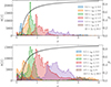 |
Fig. 5. Redshift distributions for each of our redshift and magnitude bins using the SE++ shear weights. Top: Distributions for the magnitude range 22 < IE < 24.5. Bottom: Same, but for the range 24.5 < IE < 26.5. The black curve shows the geometric lensing efficiency, β(z), with the corresponding axis plotted on the right. |
4. Weak lensing shape measurements
Weak lensing analyses require accurate measurements of galaxy shapes. The primary method designated to be used for this task in Euclid’s first main data release (DR1) is the new forward modelling method LensMC (Euclid Collaboration: Congedo 2024). To demonstrate its performance on early Euclid data, we employed LensMC in this ERO analysis, as detailed in Sect. 4.1. However, LensMC has not been used in published works analysing real imaging observations so far. Therefore, we decided to compare the LensMC-based analysis to WL constraints obtained using other shape measurement algorithms, thereby providing an empirical cross-check. For this, we in particular employ a pipeline based on the KSB+ formalism (Kaiser et al. 1995; Luppino & Kaiser 1997; Hoekstra et al. 1998), which has been applied to similar datasets in the past, as detailed in Sect. 4.2. As explained in Sect. 4.3 and Appendix A, we additionally obtained shape estimates using SourceXtractor++ (Bertin et al. 2022; Kümmel et al. 2022, abbreviated as SE++), which we also used for the photometric measurements (see Sect. 2.4). Because of different selections, these methods yield different number densities of WL source galaxies7, as summarised in Table 4 and Fig. 6. We present a first comparison of the resulting shear estimates via a matched catalogue analysis in Sect. 4.4. A more quantitative comparison is provided in Sect. 6.3.2 via the inferred WL mass estimates. In contrast to a matched catalogue analysis the latter properly accounts for the impact of shape weights and avoids a potential risk to compromise the calibration of one method by imposing additional selections from the other methods.
 |
Fig. 6. Number density of objects in the LensMC (dashed), SE++ (solid), and KSB+ (dotted) WL source catalogues, computed within the central |

Overview of the shear catalogues, including the sections providing detailed descriptions and the source densities, ngal, in the total catalogue, as well as in the IE ranges of our analysis and the nominal EWS.
Given the limited space, we show illustrative figures related to the shear catalogue creation in this section for the KSB+ method only. The PSF model employed for the other methods was already presented in Sect. 2.5. Further plots related to the SourceXtractor++ analysis and the LensMC shear calibration are provided in Appendices A and B, respectively.
4.1. LensMC
LensMC is a forward modelling shape measurement method that accounts for the PSF convolution and samples the posterior distribution of galaxy parameters via a Markov chain Monte Carlo analysis (Euclid Collaboration: Congedo 2024, hereafter C24). The method was designed specifically to meet the stringent requirements of Euclid and Stage IV WL surveys, both in terms of cosmic shear accuracy and computational scalability to measure 1.5 billion galaxies. It is now the designated shape measurement method for the Euclid data release 1 (DR1).
Since C24 LensMC has gone through substantial testing on these data, as well as early science operation data. Examples of changes are the correction of background gradients (in addition to the median) at the scale of the postage stamp extracted around the target galaxy or group of neighbouring galaxies (512 pixels in size). This helps to further mitigate any residual gradients (left over by the image reduction) that would impact our lensing measurements. Additionally, we now have much better control of outliers that are taken care of by robust sigma clipping. This helps to control the impact of residual cosmic rays or unmasked detector features. Bright star masks are also included in the measurement. LensMC takes in the SE++ photometric catalogue and uses the estimated world coordinates, object IDs, segmentation map, and PSFEx model to measure object shapes, positions, sizes, fluxes, magnitudes, χ2 values, S/N values, and parameter errors in a bulge+disc forward-modelling approach. As described in C24, objects are grouped with a friends-of-friends algorithm with a scale of 1″ and are jointly measured if belonging to the same group. LensMC flags objects (and therefore assigns them zero weight) if they are too close to masked pixels, when the segmentation map IDs are not consistent with the objects, or in case of general failures. We defined a selection function based on the measured total flux-averaged half-light radius. After checking the distributions, we implemented the star-galaxy separation by selecting objects that have a half-light radius larger than  . At the same time we removed faint galaxies with very large (and often non-physical) size estimates, which can occur for very noisy objects. The magnitude-dependent selection that we adopted for this keeps objects with a half-light radius of less than
  . This selection excludes all objects with a half-light radius larger than
  at IE = 24, but this limit increases steadily as the galaxies become larger and brighter. Shear weights are defined as in C24. All objects that were flagged or excluded by the selection above were assigned zero weight because they were deemed unsuitable for the WL analysis.
C24 conducted tests on WL image simulations based on the Euclid Flagship simulations (Euclid Collaboration: Castander 2025) mimicking data from the VIS instrument (Euclid Collaboration: Cropper 2025). However, these simulations only considered weak reduced shears (|g| = 0.02), as would be adequate in the cosmic shear regime. In order to conduct first tests of LensMC in the cluster shear regime, we analysed an additional set of image simulations with input shears |g|≤0.2, as detailed in Appendix B. Based on these tests we found that shear biases behave largely linearly for LensMC in this extended regime, which is why a standard linear multiplicative bias correction is sufficient for our study. Through these tests we also identified a dependence of the estimated multiplicative bias on details of the PSF model, including its sampling. For future Euclid WL studies, the Euclid Science Ground Segment is developing and calibrating a physical, forward-modelling, super-resolution model of the Euclid PSF, which was, however, not yet available for this analysis. We therefore employed the PSFEx PSF model described in Sect. 2.5 for this ERO analysis, sampled at the native VIS pixel scale, with a refined multiplicative shear bias correction as detailed in Appendix B. For the current study, we considered a conservative 3% uncertainty for the multiplicative bias correction to account for potential differences between the data and calibration simulations regarding the PSF model and source population properties. Following Li et al. (2023) the shear calibration for the Euclid DR1 will apply a vine-copula remapping to ensure matching source populations (Jansen et al., in prep.). Together with the improved PSF models, as well as corrections for the impact of complex galaxy morphologies (Euclid Collaboration: Csizi 2025), that work will enable a much tighter shear calibration, which was however not yet available at the time of this ERO analysis.
We note that our current analysis does not account for the impact of the SED dependence of the PSF (Cypriano et al. 2010; Eriksen & Hoekstra 2018). As detailed in Sect. 4.2, we estimate that this adds an additional 1.2% systematic uncertainty to the multiplicative shear calibration, which we add in quadrature, yielding a total multiplicative shear bias uncertainty of 3.2%. This uncertainty is fully sufficient for our single-target study, which is dominated by statistical uncertainties (see Sect. 6.3.2).
As in C24, we carried out a number of validation checks, including testing the reduced χ2 distribution, which is a very useful diagnostic of the stability of the measurement. This distribution peaks at 1.0 with a small residual positive skewness, as expected for real data in the case of adequate modelling and error estimation. Validating the distributions also informed the selection we applied to the catalogue, as discussed above.
Figure 6 shows the number counts of objects in the catalogues from LensMC and the other shape measurement methods after applying shape selections and removing objects in masked areas. The total source density7 in the correspondingly filtered LensMC catalogue amounts to 110 arcmin−2, of which 22 arcmin−2 have IE < 24.5, and 82 arcmin−2 fall into the interval 22 < IE < 26.5 employed in our WL analysis. We note that the LensMC shape catalogue extends noticeably beyond the depth limit IE < 26.5 imposed by the photometric redshift analysis (see Sect. 3).
4.2. KSB+
We also generated a WL catalogue using the KSB+ formalism (Kaiser et al. 1995; Luppino & Kaiser 1997; Hoekstra et al. 1998), employing the implementation from Erben et al. (2001) as detailed in Schrabback et al. (2010). This pipeline is also used for shape measurements in cluster WL analyses by Schrabback et al. (2018a,b, 2021), Thölken et al. (2018), and Zohren et al. (2022). We employ the correction for multiplicative WL shear estimation bias derived by Hernández-Martín et al. (2020, hereafter H20) for this KSB+ implementation, accounting for the bias dependence on S/NKSB, which is measured including the KSB+ weight function (see Erben et al. 2001; Schrabback et al. 2007). H20 tune their image simulations such that they closely resemble deep Hubble Space Telescope (HST) WL data with a resolution of 0 1 (PSF FWHM) based on observations from the Cosmic Assembly Near-IR Deep Extragalactic Legacy Survey (CANDELS, Grogin et al. 2011; Koekemoer et al. 2011), including realistic clustering. They also explored an alternative scenario matching the properties of WL data from the Very Large Telescope (VLT) High Acuity Wide field K-band Imager (HAWK-I), with a PSF FWHM of 0
 4. In this context, H20 found that multiplicative shear biases shift by less than 0.9% compared to the HST-like set-up, suggesting a low sensitivity of the calibration to the exact simulation details. Accordingly, we expect that this calibration is also applicable to the Euclid ERO observations, which have a resolution approximately at the geometric mean of the scenarios explored by H20. Based on their analysis, H20 estimate a residual systematic uncertainty of their derived multiplicative shear bias calibration of 1.5%. Similarly to the LensMC analysis we inflate this uncertainty to 3% to account for differences in both the PSF shapes and the source background selection compared to H20.
We note that H20 reported no indications of significant non-linear shear biases for reduced shears up to |g|< 0.4 for this KSB+ implementation, allowing us to safely ignore non-linear corrections at the accuracy requirements of this ERO analysis. Interestingly, this differs from the results obtained by Jansen et al. (2024), who find a significant non-linear bias component for the galsim (Rowe et al. 2015) KSB+ implementation, suggesting a dependence on the detailed KSB+ implementation differences.
Figure 7 shows the distribution of measured objects in the unfiltered KSB+ catalogue as a function of the half-light radius, rh, and S/NKSB. In the figure, the red box indicates the cuts that are used to select stars for the PSF modelling, where we exclude not only faint and noisy stars, but also brighter stars to avoid the impact of non-linear effects such as the brighter-fatter effect (Guyonnet et al. 2015). The selected stars have a median half-light radius of  as measured by analyseldac (Erben et al. 2001), as well as median values of the flux radius and the FWHM, as measured by SExtractor (Bertin & Arnouts 1996) of
  and
and  , respectively.
 |
Fig. 7. Distribution of S/NKSB versus rh for objects in the unfiltered KSB+ catalogue. The red box and blue lines indicate the pre-selection regions for the stars that are employed in the PSF modelling and for the galaxies, respectively. For clarity only a random sub-set of 20% of catalogue entries is displayed. Stars and noisy or poorly resolved galaxies are further removed from the shear catalogue via cuts in photometric redshift, magnitude, the SExtractor S/N, and additional KSB+ selections (see H20). |
The selected stars were used to obtain local estimates of PSF parameters, such as the components of the KSB+ PSF polarisation eα, measured as a function of the KSB+ Gaussian filter scale, rg. We find that the PSF properties as measured with KSB+ vary fairly smoothly across the relevant part of the VIS image stack, which is why we employed a simple third-order polynomial interpolation for the current study (see Fig. 8). We note that the overall level of PSF ellipticity is quite low. In particular, when it is measured with a Gaussian filter scale of  (as employed for typical compact galaxies), the root-mean-square (rms) of the polarisation model amounts to only 2.7% when combining both polarisation components and averaging over the area depicted in Fig. 8.
 |
Fig. 8. Spatial variation of the PSF polarisation eα measured using a KSB+ Gaussian filter scale |

The blue lines in Fig. 7 indicate lower limits  and S/NKSB, min = 2 employed in the galaxy selection. The source selection furthermore includes cuts in KSB+ parameters (see H20), as well as S/Nflux > 8, which is well-bracketed by the scenarios tested by H20. Figure 6 compares the number counts of objects in the catalogues from KSB+ and the other shape measurement methods after applying the corresponding shape selections and removing objects in masked areas. The total source density7 in the correspondingly filtered KSB+ catalogue amounts to 74 arcmin−2, of which 18 arcmin−2 have IE < 24.5 and 65 arcmin−2 fall into the interval 22 < IE < 26.5 employed in our WL analysis. Compared to the other shape catalogues the source density is somewhat lower for the KSB+ catalogue. This is due to a combination of several factors, including a more conservative removal of both objects with close neighbours and galaxies that are noisy or poorly resolved. Large galaxies are also removed within the employed KSB+ pipeline if they are not well covered by the internal postage stamp cutout.
Figure 9 shows the dispersion, σϵ, α, of the measured ellipticity estimates from all objects in the fully filtered KSB+ galaxy catalogue, split into bins of IE. Combining both ellipticity components ϵ1 and ϵ2, we fit these values with a third-order polynomial interpolation (smooth curve in Fig. 9) in order to define an empirical shape weight of wi = [σϵ(IE)]−2 (e.g. Schrabback et al. 2018b).
 |
Fig. 9. Dispersion of the fully corrected KSB+ ellipticity estimates as a function of IE magnitude, shown for both ellipticity components ϵ1 and ϵ2. The smooth curve shows the best-fit third-order polynomial interpolation function, which is used for the computation of the empirical shape weight. |
In this work, we neglected the impact of the SED dependence of the PSF (Cypriano et al. 2010; Eriksen & Hoekstra 2018) for all shape catalogues. To assess the impact of this, we employed the formalism from Cypriano et al. (2010, as expressed in their Eq. A7). For this, we computed the required size ratio of the PSF and the galaxies via the corresponding flux radii from SExtractor, averaged over all selected galaxies in the KSB+ catalogue. The resulting effective shift in the multiplicative shear bias depends on the difference in the FWHM of the effective PSFs for stars and galaxies. When assuming the corresponding estimates by Cypriano et al. (2010) for the average galaxy population versus a typical disk or halo stars, we obtained a shift in the multiplicative bias by 1.2% or 0.8%, respectively. We use the larger one of these values as estimate for the resulting multiplicative bias uncertainty, which we add in quadrature to the 3% estimate discussed above, yielding a joint uncertainty of 3.2%.
4.3. SourceXtractor++
In our work, SE++ is not only employed for photometric measurements (see Sect. 2.4), but also as one of the methods to obtain PSF-corrected galaxy shapes for the WL analysis. Differing from the photometric analysis, this separate SE++ run employs a single Sérsic profile, directly providing an ellipticity estimate, as well as best-fit sizes for the star-and-galaxy discrimination. Recent tests done as part of the Euclid Morphology Challenges (Bretonnière 2023; Euclid Collaboration: Merlin 2023) indicate that SE++ can not only recover accurate multi-band photometry, but also morphological parameters including ellipticity, orientation, Sérsic index, and half-light radius. Likewise, earlier tests conducted by Mandelbaum et al. (2015) and Euclid Collaboration: Martinet (2019) demonstrated that SExtractor’s model-fitting engine can reach an accuracy that is sufficient for Stage III WL surveys. However, we note that SE++ has not yet gone through the same level of testing on WL image simulations as the other two shape measurement methods employed in this study. We therefore regard the constraints from the other methods as primary results, where the comparison to the SE++ constraints provides a data-driven validation for the SE++ implementation.
As in the case of the other two shape measurement methods, galaxy ellipticities are better measured for high-surface-brightness extended sources. Noise and PSF blurring induce more uncertain ellipticity, which must be properly accounted for in a weighting scheme. The recovered uncertainties on the ϵ1 and ϵ2 ellipticity components are added in quadrature to a constant shape noise floor σϵ, 0 ≡ 0.25 in order to down-weight poorly constrained galaxy shapes. Appendix A provides further details on our employed SE++ implementation.
For the different shape catalogues the number counts of objects, after applying shape selections and removing objects in masked areas, are compared in Fig. 6. The total source density7 in the correspondingly filtered SE++ catalogue amounts to 126 arcmin−2, of which 29 arcmin−2 have IE < 24.5 and 102 arcmin−2 fall into the interval 22 < IE < 26.5 employed in our WL analysis.
4.4. Raw shear profile comparison
As a consistency test, we conducted a first comparison of the shear signal probed by the three shear catalogues in this subsection. The catalogues differ in their depth and weighting, which affects the expected shear signal and will be accounted for in the full analysis presented in Sect. 6.3. For this first test presented here we limit the catalogues to the joint sample of sources that have non-zero shape weights for all three shape measurement methods. We then computed the tangential component as
 (1)
(1)
and the cross-component as
 (2)
(2)
of the reduced shear estimates, where ϕ denotes the azimuthal angle with respect to the cluster centre (see Sect. 6.3 regarding the choice of centre). We compare their averages as a function of the physical (not co-moving) radial distance r from the cluster centre for the three shear catalogues in Fig. 10, finding very good agreement both for the tangential component and the cross component. The latter is consistent with zero for all three shape catalogues, as expected in the case of accurately removed instrumental signatures. As a further check we split the matched source sample into bins of galaxy size, likewise finding good agreement between the three catalogues in terms of the resulting reduced shear profiles.
 |
Fig. 10. Matched-sample comparison of the raw reduced shear profiles (prior to the background selection and contamination correction) obtained from the three shape catalogues, showing both the tangential component ⟨gt⟩ and the cross-component ⟨g×⟩. In the average computation we only include sources that have non-zero shape weights as computed by all three methods. The error bars include shape noise and are therefore correlated between the methods, explaining why the tangential reduced shear profiles obtained by the three methods differ from each other to a lesser extent than the error bars. For the KSB+ catalogue ⟨gt⟩ is plotted at the correct position, while the other data points have been offset along the x-axis for clarity. |
5. Quantifying and correcting for cluster member contamination
Cluster members constitute an excess population compared to random galaxy populations that are used to estimate the source redshift distribution (see Sect. 3.2.2). Accordingly, it is necessary to accurately estimate the radius-dependent contamination of the selected source galaxies by cluster members, in order to correct the estimated shear signal for the dilution caused by this contamination. Here, we determined this correction based on the number density profile (Sect. 5.1), which, however, needs to be corrected for the impact of source obscuration (Sect. 5.2) and lensing magnification (Sect. 5.3). Similarly to Kleinebreil et al. (2025) we conducted this contamination analysis in the same photometric redshift bins as used for the redshift calibration, since we expected to find a dependence of the contamination level on the source photo-z and magnitude.
5.1. Source number-density profile
For all combinations of photo-z and magnitude bins (see Sect. 3.2) we calculate the radial source number-density profile in geometric annuli, which mirror the binning of the shear measurement (see Sects. 4.4 and 6.3). Here, we take the masked fraction, fmasked, of each annulus into account and compute the corresponding number densities and Poisson errors,
 (3)
(3)
 (4)
(4)
where r1 and r2 are the inner and outer radii of the annulus, Ngal is the number of sources in a given bin, and fmasked is the geometric masked fraction. We show the resulting number density profiles in Fig. 11. The bins with low photometric redshifts zph show a pronounced increase in source number density towards the cluster centre, which is expected due to cluster member contamination. On the other hand, some of the high-redshift bins show a noticeable drop below 1 Mpc, which is likely due to the optical obscuration caused by bright cluster galaxies and possibly magnification (see Sects. 5.2 and 5.3). Contamination generally appears to be stronger for the bright sample (22.0 < IE < 24.5), and obscuration seems to affect the faint sample (24.5 < IE < 26.5) more strongly.
 |
Fig. 11. Number density profiles of WL sources in bins of photo-z (colour-coded) and magnitude, where the solid and open symbols correspond to the bright and faint sample, respectively. Error-bars indicate Poisson uncertainties. In this figure, we account for masked areas, but not for obscuration. |
5.2. Estimation of and correction for source obscuration
Bright cluster galaxies can cause significant optical obscuration and impede the ability to detect background galaxies along and close to their lines of sight. To extract an accurate cluster member contamination model from source number density profiles, we therefore need to take the obscuration effects of the lens into account. We modified the image injection pipeline described in Kleinebreil et al. (2025) for this task.
We generated galaxy images with GalSim (Rowe et al. 2015) based on galaxy properties that we drew randomly from the Flagship catalogue (Euclid Collaboration: Castander 2025). In particular, we generated double-Sérsic profile models based on the Flagship galaxy properties (which model the disc and the bulge of a galaxy) and convolved the resulting image with a Euclid-like optical PSF following Tewes et al. (2019) and Jansen et al. (2024). We subsequently injected the simulated galaxy stamps into the real VIS observations at random positions and at a density of 3 arcmin−2 within the Flagship VIS magnitude interval 20 < IE < 24.5 per injection run. This is equal to 10% of the nominal number density of the EWS. Towards fainter magnitudes we inject sources based on the Flagship magnitude distribution with the same fraction, leading to an overall galaxy injection density of 29.4 arcmin−2.
Following the source injection, we re-ran the object detection using SourceExtractor (Bertin & Arnouts 1996), employing identical settings as used for the generation of the WL source catalogue. Since we knew the injected objects’ positions, we were able to calculate their detection probability (as the ratio of the numbers of re-detected and injected galaxies). We show a high-resolution map of the resulting detection probability in Fig. 12.
 |
Fig. 12. Overlaid with the monochrome VIS image of Abell 2390, the colour coding shows the detection probability map of the whole injection input sample in the inner 4 Mpc × 4 Mpc, with no selection in input magnitude, photo-z, or other quantities applied. The image injection pipeline captures cluster galaxies and foreground stars including their diffraction spikes. |
We injected 107 galaxy images in total, which we split into three injection areas (or ‘batches’) to compensate for the increasing geometric area of equidistant annuli. The first batch of injection runs covers the full 8 Mpc × 8 Mpc of the observed cluster field and consists of 422 individual runs that provide a total of 4 × 10⁶ injected galaxy image stamps into the VIS image. The second batch covers an intermediate area of the central 4 Mpc × 4 Mpc, where we again inject 4 × 10⁶ image stamps over 1686 injection runs. The third batch only covers the inner 2 Mpc × 2 Mpc of the cluster, where we inject 2 × 10⁶ image stamps over 3373 injection runs. Each injection run in these three batches has the same galaxy injection density of 29.4 arcmin−2.
The effect that foreground cluster galaxies have on the detection probability of background sources is expected to depend on the brightness of the background sources. Therefore, we use the same split into magnitude bins that we employ for the WL analysis (22.0 < IE < 24.5 and 24.5 < IE < 26.5; see Sects. 3.2 and 6.1). Given a potential additional dependence on size and S/N, we additionally mimicked the corresponding selections of the KSB+ analysis using SExtractor-measured quantities. In the injection analysis we do not find a significant additional dependence of the detection probability on the input photo-z from the Flagship catalogue. We therefore do not apply a further sub-selection into photometric redshift bins. Figure 13 shows the resulting detection probability profile for the two magnitude bins, normalised to the mean of the values of the three outermost bins, which we regard as the field value. Here, the high-resolution VIS mask has been taken into account. The density of re-detected injections decreases rapidly below a cluster-centric distance of 1 Mpc, especially in the fainter magnitude bin, which we attribute to the increasing spatial density of cluster galaxies. The innermost annulus shows a sharp drop in detection density, likely due to the brightest cluster galaxy (BCG). We note an additional intermediate dip at r ≃ 2.5 Mpc. We speculate that this may be caused by Galactic cirrus present in this area. To test this hypothesis we created a rudimentary cirrus mask and observe that the dip in detection density in this radial range corresponds well to the mask’s radial profile (compare to Fig. 13).
 |
Fig. 13. Relative spatial density of re-detected galaxies with a Flagship redshift in the range 0.3 < zobs < 2.8 that fulfil the WL selection cuts. We show the contribution of a rudimentary cirrus mask to the unmasked area of each annulus, scaled by |

5.3. Accounting for magnification
Massive cluster haloes cause redshift-dependent lensing magnification, which affects the observed source number density in several ways (e.g. Schrabback et al. 2018a). Firstly, it increases the observed separation between objects, thereby reducing the number density of sources. Moreover, the observed galaxy images increase in size. This can change the source selection if an analysis employs a size cut, which is the case in this work. The size change may additionally affect the lensing weights derived from shape measurements. We ignored this second-order correction here, but suggest that its impact is investigated for future studies that analyse larger cluster samples and have tighter accuracy requirements. Lastly, the brightness of the sources increases because of magnification, changing the number of galaxies in a given magnitude bin.
We computed an approximate correction for the combined impact that magnification has on the source number density profile with the help of the Flagship catalogue. We note that we did not follow the often employed simplified treatment of magnification via the slope of the number counts (e.g. Broadhurst et al. 1995). Instead, we applied an artificial magnification to a full Flagship-based galaxy population to account for the range of effects listed in the previous paragraph.
In particular, we selected 107 Flagship galaxies randomly and divide them into tomographic redshift bins based on the ‘observed’ redshift zobs (including peculiar velocities) in the Flagship catalogue. We assumed a reference Navarro-Frenk-White (NFW, Navarro et al. 1997) density profile with M200c = 1.5 × 10¹⁵ M⊙ and c200c = 4 (consistent with earlier studies of the cluster; see Applegate et al. 2014; Okabe & Smith 2016; Herbonnet et al. 2020, and Sect. 7.1) to compute the radius-dependent magnification for each galaxy in the Flagship sample following Schrabback et al. (2018a) as
 (5)
(5)
where we employ the ‘true’ redshift (without peculiar velocity) as the source redshift, zs. Next, we have the geometric lensing efficiency,
 (6)
(6)
which depends on the angular diameter distances between the observer and the source Ds, as well as the lens and the source Dls, respectively. Here, H(zs − zl) denotes the Heaviside step function, which is equal to one for sources with zs > zl and vanishes otherwise. In Eq. (5) β0 is an arbitrary fiducial lensing efficiency, which we calculate at the central redshift of each tomographic bin, and κ0(r) is the corresponding convergence at this redshift. Magnification changes galaxy sizes and magnitudes according to
 (7)
(7)
 (8)
(8)
We approximately mirrored the KSB+ source selection in terms of cuts in (lensed) half-light radius and S/Nflux, and then count the galaxies in the un-lensed and the lensed sample, for both the bright and faint magnitude bins. We additionally included a weight W = 1/μ(ztrue) < 1 for each galaxy in the magnified sample to account for the magnification of the observed sky area. The ratio of the two number counts then yields an estimate for the impact that magnification has on the source number densities. We show the resulting radial profiles for the different bin combinations in Fig. 14.
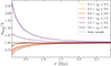 |
Fig. 14. Impact of magnification on source number densities for our set-up and an M200c = 1.5 × 10¹⁵ M⊙, c200c = 4 NFW halo. The solid and dashed lines show the bright (22.0 < IE < 24.5) and faint (24.5 < IE < 26.5) samples, respectively. |
We stress that our use of the Flagship mock catalogue for magnification modelling only assumes that the Flagship galaxy distribution as a function of magnitude, size, and redshift provides a good match to the corresponding distribution of galaxies in the real universe. This was indeed tested and confirmed by Euclid Collaboration: Castander (2025) via the comparison of Flagship and COSMOS galaxy samples.
5.4. Cluster member contamination
We use the estimated detection probability profiles from Sect. 5.2 to boost the radial source density profiles on a bin-by-bin basis. We decide against a model fit of the detection probability profiles, because we can capture the intrinsic obscuration fingerprint of the cluster (and Galactic cirrus) in this way. We show the resulting detection bias-corrected source number density profile in Fig. 15, normalised to the mean value of the three outermost bins. We fit an exponential profile,
 (9)
(9)
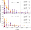 |
Fig. 15. Source number density profiles after correction for the impact of source obscuration and magnification, scaled to the corresponding mean value of the three outermost annuli. The increase over the baseline is a direct measure of the boost factor that we need to apply to compensate for cluster member contamination. We show an exponential model fit as dashed (22.0 < IE < 24.5) and dotted (24.5 < IE < 26.5) curves. |
to the corrected source number density profiles, where a separate amplitude A is fit for each magnitude and photometric redshift bin combination, while the scale radius rS = (350 ± 39) kpc is jointly constrained from all bin combinations. This model is a direct measure of the boost factor that we apply to the shear measurement. We show the resulting contamination 1 − nouter/n(r) for the KSB+ source sample in Fig. 16.
 |
Fig. 16. Contamination profiles for the KSB+ lensing sample based on the fits of the obscuration- and magnification-corrected radial source density profiles for the different tomographic redshift and magnitude bin combinations. Dashed lines correspond to the bright sample (22.0 < IE < 24.5), while dotted lines show the profiles for the faint sample (24.5 < IE < 26.5). The shaded areas represent the ±1σ uncertainties of the model fit. |
6. Weak lensing results
6.1. Source bin selection and average lensing efficiencies
In the contamination analysis presented in Sect. 5, we considered a total of six photometric redshift bins. For the main WL results presented here, we dropped both the bin with 0.2 < zph < 0.3, which includes the cluster redshift, and the highest photometric redshift bin 2.8 < zph < 6.0. The latter bin was removed since it does not contribute significant constraining power, containing only few sources, while suffering from both cross-contamination in the n(z) calibration (see Sect. 3.2) and large uncertainties regarding the contamination model (see Fig. 16). We report the average geometric lensing efficiency ⟨β⟩, as well as ⟨β2⟩ for the remaining four photometric redshift bins and both magnitude bins in Table 5, taking the shape weights of the different shear catalogues into account. Galaxies for which the source redshift distribution cannot be calibrated (see Sect. 3.2.2) are dropped both for this computation and for the analyses presented in the following subsections.
Average lensing efficiency values ⟨β⟩ and ⟨β2⟩ computed for the different magnitude and photo-z bin combinations using the shear weights w from LensMC, SE++, and KSB+, respectively.
6.2. Weak lensing convergence reconstruction
The WL convergence, κ = Σ/Σcrit, is defined as the ratio of the surface mass distribution, Σ, and the critical surface mass density
 (10)
(10)
which is given in terms of the gravitational constant, G, the light speed, c, the angular diameter distance to the lens, Dl, and the geometric lensing efficiency, β (see Eq. (6)).
Since the WL convergence, κ, and shear, γ, are second-order derivatives of the lensing potential (Bartelmann & Schneider 2001), reconstructions of the κ distribution can be estimated from the shear field up to an integration constant known as the mass-sheet degeneracy (Falco et al. 1985; Schneider & Seitz 1995). For the reconstruction we employ a Wiener-filtered algorithm following McInnes et al. (2009) and Simon et al. (2009), as described in more detail in Appendix C. In the reconstruction we set the mean convergence in the field to zero to fix the mass-sheet degeneracy. This can lead to noticeable κ underestimations for small field sizes (e.g. Schrabback et al. 2021), but is less of an issue for the wide field covered by the Euclid observations and complementary ground-based data. Also note that we do not use the κ reconstructions shown in Figs. 17 and 18 (as well as Figs. D.1 and D.2) for quantitative constraints, but rather only for illustration purposes.
 |
Fig. 17. Convergence κ reconstructions based on the LensMC (left), KSB+ (middle), and SE++ (right) shear catalogues, showing the E mode (top) and B mode (bottom). Contours are spaced in steps of Δκ = 0.03 starting at κ = 0.03. |
When fully corrected for shape measurement and selection biases, the galaxy ellipticity estimates provide unbiased estimates for the reduced shear, which is linked to the (unobservable) shear, γ, and convergence, κ, as
 (11)
(11)
Given the high cluster-mass scale and lensing efficiency, the distinction between shear and reduced shear cannot be neglected for our study. For the quantitative mass constraints presented in Sect. 6.3 we correctly model the reduced shear from the redshift-dependent shear and convergence. For the convergence reconstructions we applied an approximate correction, scaling first the individual boost-corrected reduced shear estimates from the different tomographic redshift bins (with 0.3 < zph < 2.8) and both magnitude bins to the same average lensing efficiency, in order to combine them into a single catalogue of sources that have non-zero shape weights and photometric redshift calibration weights. We then conduct the convergence reconstruction iteratively, applying a conversion from reduced shear to shear based on the convergence map of the previous iteration.
Figure 17 shows the convergence reconstructions over the area covered by the Euclid and photometric data for the three different shear catalogues in the top panels (E mode). The bottom panels show the corresponding B-mode reconstructions, for which galaxy ellipticities have been rotated by 45°, providing an estimate for the level of noise and potential residual systematics in the reconstruction (e.g. Massey et al. 2007). Based on the comparison of the E-mode and B-mode reconstructions, Fig. 17 shows that the cluster is detected with high significance for all three shear catalogues. All reconstructions show very similar morphologies, with a significant elongation approximately along the south-east to north-west direction. This can be compared to the Euclid optical+NIR colour image of the cluster via the overlay presented in Fig. 18 for the LensMC analysis, and in Figs. D.1 and D.2 for the other shear catalogues. This shows that the κ contours trace the distribution of cluster galaxies well for all three reconstructions, especially in the inner cluster region. These figures also show that the central peaks of the reconstructions closely coincide with the BCG.
 |
Fig. 18. Overlay of a Euclid HEYEIE colour image of A2390 with the Wiener-filtered E-mode κ reconstruction shown as contours in steps of Δκ = 0.03, starting at κ = 0.03, as derived from the LensMC shape measurements. For illustration the magenta whiskers show the estimated shear field binned on a coarse grid without applying smoothing (a finer grid is used to compute the κ reconstruction; see Appendix C). |
6.3. Weak lensing mass constraints
6.3.1. Shear profile fitting
To derive WL mass constraints for the cluster, we employed the sources of both magnitude bins and the four tomographic redshift bins with 0.3 < zph < 2.8 that are characterised by non-zero weights both in the shape analysis and photo-z calibration. We computed tangential reduced shear profiles separately for each photometric redshift and magnitude bin combination, but jointly fit all bins with a single spherical NFW (Navarro et al. 1997) mass model, for which we computed tangential reduced shear profile predictions according to Wright & Brainerd (2000). Here, we account for the correct ⟨β⟩ for each bin combination and also apply corrections for the finite width of their redshift distributions based on the estimated ⟨β2⟩ following Seitz & Schneider (1997), Hoekstra et al. (2000), and Applegate et al. (2014).
For the mass constraints we employ the radial fit range 0.5 Mpc ≤ r ≤ 3.3 Mpc. This avoids increased systematic uncertainties that occur both in the core region, where the contamination correction has the largest impact, and at very large scales, where deviations from a single NFW model are expected due to neighbouring structures (e.g. Grandis et al. 2024).
For noisy WL data the centring of shear profiles poses a significant challenge for accurate mass measurements. For example, when centre proxies such as the X-ray centroid, the peak in the Sunyaev-Zeldovich-effect (SZE, Sunyaev & Zel’dovich 1970) signature, or the BCG candidate are used, significant offsets can occur (e.g. Schrabback et al. 2018a). This can lead to biased mass constraints even when corrections for isotropic miscentring distributions are applied (Sommer et al. 2024), although Sommer et al. (2025) find that this problem can be mitigated by modelling the miscentring with respect to the centre of mass. Likewise, substantial biases occur when centring shear profiles directly on noisy reconstructed WL convergence peaks (Sommer et al. 2022). However, for our study, this is not an issue, since the mass centre of the cluster is very well constrained, both by the WL data themselves (see Sect. 6.2) and by strong lensing constraints of the core region. In particular, the joint strong and WL analysis presented in our companion paper (Diego et al. 2026) precisely constrains the cluster mass centre to the position  located about 6″ southeast from the BCG. This provides a centre for our shear profile analysis with negligible uncertainty, which is used throughout our analysis unless noted differently.
When fitting NFW models for individual clusters, WL studies often employ a concentration–mass relation (e.g. Herbonnet et al. 2020; Schrabback et al. 2021) or a fixed concentration (e.g. von der Linden et al. 2014b) given the limited constraining power and radial fit range of the data. Here, we also follow this approach and assume a fixed concentration c200c = 4 consistent with von der Linden et al. (2014b), leaving the mass M200c as the only free parameter (constraints on both mass and concentration derived from joint strong and WL modelling are presented in Diego et al. 2026). As usual, we employed over-density masses MΔc, which are measured in spheres with radius rΔc, within which the average density is equals Δ times the critical density of the Universe at the cluster redshift.
6.3.2. Resulting mass estimates and uncertainties
We summarise the resulting mass constraints for the three shape catalogues in Table 6, including also derived mass constraints for Δ = 500. In addition to the shape noise caused by the intrinsic galaxy shapes, statistical uncertainty in cluster WL is also caused by large-scale structure projections (e.g. Hoekstra 2001). We estimate these by computing Gaussian shear field realisations for the broad combined redshift distribution of our tomographic bins following Appendix B in Simon (2012) and modelling the non-linear matter fluctuation power spectrum according to Takahashi et al. (2012) assuming our reference cosmology. As a result we find that large-scale structure projections actually provide a larger contribution (11% relative uncertainty) to the statistical error budget for our dataset compared to shape noise (8% relative uncertainty).
WL mass constraints for Abell 2390 assuming a spherical NFW mass model with fixed concentration c200c = 4, where the first and second uncertainties listed correspond to the statistical uncertainties from shape noise and large-scale structure projections, respectively (see Sect. 6.3.2 for systematic uncertainties).
Compared to the combined 14% statistical uncertainty the systematic uncertainty is small for our study. The largest contribution originates from the shear calibration, where the 3.2% calibration uncertainties estimated for the KSB+ and LensMC catalogues (see Sect. 4) translate into 4.8% mass uncertainties. While the employed SE++ implementation has not yet gone through the same level of testing on WL image simulations, the excellent agreement, especially with the KSB+ catalogue (see also Sect. 4.4), empirically demonstrates a similar level of shear calibration uncertainty for SE++.
A further source of systematic mass uncertainty is provided by the uncertainty of the contamination correction (see Sect. 5.4). We estimate this by varying the contamination correction parameters within their fit uncertainties and refitting the WL cluster mass. Here we find that the residual uncertainty of the contamination correction leads to a 0.7% systematic mass uncertainty only, which is negligible compared to the other uncertainties.
Finally, uncertainties in the procedure to calibrate the true source redshift distribution (see Sect. 3.2) will further contribute to the systematic mass uncertainty. A full quantification of this uncertainty requires a realistic end-to-end simulation of the redshift calibration data and calibration procedure. Efforts in this direction are underway within the Euclid Consortium (see Roster et al. 2026), but this is far beyond the scope of our current paper. However, to provide at least an approximate estimate of the level of uncertainty, we have bootstrapped the calibration sample from COSMOS2020 and computed the dispersion of the estimated mean redshifts in the different combinations of magnitude and photometric redshift bins. For the bin combinations included in the WL mass analysis, this dispersion is in the range of σ(⟨z⟩) = 0.006–0.031. Even if we conservatively assume that these shifts are maximally correlated between the different bin combinations, their joint impact still shifts the estimated cluster masses by less than 0.4%. This weak sensitivity to redshift errors is thanks to the fact that most of the constraining power comes from the higher-redshift tomographic bins (0.9 < zph ≤ 1.5 and 1.5 < zph ≤ 2.8), where the geometric lensing efficiency β depends only weakly on source redshift, given the fairly low cluster redshift (see Fig. 5). We note that this uncertainty estimate does not include the impact of potential systematic uncertainties in the calibration data itself. Regarding such systematic uncertainties, similar previous deep WL studies employing a deep and well-calibrated photometric redshift catalogue as reference sample, found that catastrophic redshift outliers between galaxies at very low redshifts and very high redshifts are the primary concern (Schrabback et al. 2010, 2018a; Raihan et al. 2020). For the current study, we circumvent this problem by not including the lowest and the highest photometric redshift bins, which are most affected by catastrophic outliers (compare Fig. 5). Thus, we expect that our estimate provides a reasonable assessment of the approximate level of systematic uncertainty related to the redshift calibration. However, given the limitations explained above, we conservatively inflate our uncertainty estimate by a factor three, yielding 1.2%.
Adding all the sources of systematic uncertainty listed above in quadrature, yields a combined 5% systematic mass uncertainty from the WL shear analysis, dominated by the shear calibration uncertainty. We remind the reader that this quoted uncertainty assumes a one-parameter spherical NFW density profile with fixed concentration c200c = 4 and accurate centring. While centring uncertainties are indeed negligible for our study given the tightly constrained centre (see Sect. 6.3.1), the assumption of a spherical NFW density profile with fixed concentration can lead to substantial additional scatter (approximately 20%; see e.g. Becker & Kravtsov 2011; Sommer et al. 2022; Euclid Collaboration: Giocoli 2024) when compared to other mass estimates8. For cosmological cluster population studies that include adequate simulation-based WL mass modelling corrections (e.g. Bocquet et al. 2024a,b; Grandis et al. 2024) this, however, only leads to scatter and not systematic uncertainty. Therefore, we chose to not include this scatter in the shear-related systematic error budget presented in this subsection (for constraints that vary both mass and concentration, see our companion paper, Diego et al. 2026).
6.3.3. Comparison of results from different catalogues and bins
As can be seen in Table 6, the WL mass constraints derived from the KSB+ and SE++ catalogues are in excellent agreement, and the LensMC best-fit mass is slightly higher. However, when considering the systematic uncertainty due to shear calibration, the LensMC and KSB+ masses also agree at the 1.2σ consistency level. We note that differences in the mass constraints are additionally caused by differences in shear weights and selections, which is why the true level of consistency is even better. In conclusion we find that the mass constraints obtained from the different shear catalogues are fully consistent.
As an important further check for the overall analysis we investigate also the consistency of mass constraints for different tomographic redshift bins and magnitude bins. Figure 19 compares the overall mass constraints indicated by the dotted blue lines to M200c estimates computed from the different magnitude and photo-z bin combinations separately (in this figure uncertainties only reflect the shape-noise component). While individually much noisier, we find that the results obtained in the individual bins agree very well with the joint constraint. This suggests that there are no strong magnitude- or photometric redshift-dependent systematic trends in the data. Only the bright (22 < IE < 24.5) galaxies in the highest tomographic redshift bin (1.5 < zph < 2.8) yield a mass constraint that is high compared to the joint constraint by about 2σ, but with a total of eight bin combinations such an outlier is not unexpected.
 |
Fig. 19. WL constraints on M200c based on the LensMC (left), KSB+ (middle), and SE++ (right) shear estimates. The dashed blue lines show the average and 1 σ uncertainty range, while the symbols show the individual constraints from the different magnitude and photometric redshift bin combinations. The black circles show the bright magnitude bins and are plotted at the bin centre with horizontal error bars indicating the bin width. The red crosses show the results from the faint magnitude bin and have been offset by Δzph = 0.02 for clarity. To translate the indicated photometric redshift ranges into estimated true redshift distributions see Fig. 5. All results assume a fixed concentration c200c = 4, with plotted mass uncertainties corresponding to shape noise only. |
The good agreement of the mass constraints obtained for the different combinations of magnitude and redshift bins provides a joint validation for the estimated shears and average lensing efficiencies, as well as the correction for cluster member contamination. The agreement is also of interest regarding the underlying assumption that intrinsic source ellipticities are uncorrelated with respect to the position of the cluster centre. This assumption is well motivated for the tomographic bins spanning the range 0.6 < zph ≤ 2.8, which are clearly dominated by background sources with very low cluster member contamination (compare Figs. 5 and 16). However, the source bins with 0.3 < zph ≤ 0.6 show a substantial contamination by galaxies associated with the cluster at small scales (see Fig. 16). A potential preferential orientation of these galaxies with respect to the cluster centre would lead to biased shear profiles and mass estimates. The excellent agreement of the mass estimates of the different source bins therefore indicates that such a potential intrinsic alignment of galaxies associated with the cluster must be small and below the detection limit. This is consistent with the findings by Sifón et al. (2015), who investigate alignments of spectroscopically confirmed member galaxies of low-redshift clusters.
The shear profiles computed in the individual tomographic redshift and magnitude bin combinations are very noisy. Therefore, we show combined profiles in Figs. 20 and 21. Here we scale profiles to the same average ⟨β⟩ of the contributing bins and also rescale model predictions accordingly. We combine the two magnitude bins for each contributing photometric redshift bin in Fig. 20. For comparison, Fig. 21 shows the combined profiles when including all photometric redshift and magnitude bins that contribute to the overall mass constraints, illustrating the overall constraining power of the data. In this figure we also show the 45°-rotated (B-mode) ⟨g×⟩ profiles, which are broadly consistent with zero, as expected in case of an accurate removal of instrumental signatures.
 |
Fig. 20. Magnitude-bin-combined contamination-corrected tangential reduced shear ⟨gt⟩(r) profiles of A2390 based on the LensMC (left), KSB+ (middle), and SE++ (right) shear estimates. For this figure, the individual noisy ⟨gt⟩(r) profiles of the two magnitude bins have been combined (slightly scaled to their average mean ⟨β⟩) to yield a single ⟨gt⟩(r) profile for each tomographic redshift bin. For each set of data points the curve plotted in the same colour shows the correspondingly averaged NFW reduced shear profile model for the jointly constrained best-fit cluster mass, assuming a fixed concentration c200c = 4. The data and model for the tomographic bin with 0.3 < zph < 0.6 is shown at the correct position, while the points and models of the other tomographic bins have been shifted consistently along the x-axis for clarity. |
 |
Fig. 21. Combined contamination-corrected reduced shear profiles of A2390 based on the LensMC (left), KSB+ (middle) and SE++ (right) shear estimates. For this figure, the individual noisy reduced shear profiles of the different magnitude and photometric redshift bins have been rescaled to the effective mean ⟨β⟩ and combined, including all tomographic bins with 0.3 < zph < 2.8. The curves show the correspondingly averaged best-fit NFW model prediction for the tangential component assuming a fixed concentration c200c = 4. |
7. Discussion
7.1. Comparison to earlier studies
An early detection of the A2390 WL signal was achieved by Squires et al. (1996), who employed images taken with the Loral 3 CCD on CFHT. These early observations were limited to a small 7′×7′ field-of-view and therefore only capable of probing the inner cluster regions. This limitation was overcome in later years via the use of wide-field imaging data. For example, the cluster was included in the Weighing the Giants project (von der Linden et al. 2014a; Kelly et al. 2014; Applegate et al. 2014), which employed imaging from Subaru/Suprime-Cam and CFHT/Megacam. Applegate et al. (2014) report constraints for Abell 2390 assuming a spherical NFW density profile with fixed concentration c200c = 4, which can directly be compared to our study. Their constraint rs = (0.56 ± 0.04) Mpc on the NFW scale radius (obtained for a colour-cut source selection) corresponds to a mass  , which is fully consistent with our derived mass constraints.
As part of the LoCuSS project, Okabe & Smith (2016) also studied the WL shear profile of A2390 using Subaru/Suprime-Cam imaging. They report a mass constraint  , in excellent agreement with our measurements9. Likewise, the cluster was part of the joint analysis of CFHT data from the CCCP (Hoekstra et al. 2015) and MENeaCS programmes by Herbonnet et al. (2020), who find M200c = (16.4 ± 3.0)×1014 M⊙, which is likewise in good agreement with our constraints10. We note that Herbonnet et al. (2020) scaled their mass estimates by a simulation-derived factor 0.93−1 to account for an average mass modelling bias for their cluster population study. Such a bias not only depends on the adopted concentration–mass relation and fit range (Sommer et al. 2022), but additionally on factors such as the dynamical state and the triaxiality (e.g. Euclid Collaboration: Giocoli 2024), which are not fully known for individual clusters. Accordingly, we do not apply a mass bias correction for our single-target study. For a more direct comparison we therefore also consider the mass M200c = (15.3 ± 2.8)×1014 M⊙ that Herbonnet et al. (2020) would have found without mass bias correction. This mass estimate is likewise fully consistent with our results. In summary, our mass constraints agree very well with recent wide-field imaging analyses that also report mass constraints assuming NFW density profiles. We note however that the Euclid constraints are tighter by factors of approximately 0.6–0.8 thanks to their higher WL source densities.
A recent publication studying the WL signature of A2390 was presented by Dutta et al. (2024), who combine shape estimates in 411 short exposures taken with the WIYN/ODI imager. Since this paper does not report spherical overdensity mass estimates we cannot compare their and our results quantitatively. Finally, first WL measurements based on the Euclid ERO observations of A2390 were already presented in the overview publication of this ERO dataset (Atek et al. 2025). That analysis employed the KSB+ measurements discussed here to present an initial convergence reconstruction based on the ERO observations. We have extended this analysis by adding two further shape catalogues, refined calibrations, a background selection using photometric redshifts, and an estimation and correction for cluster member contamination. The latter two items increase the measured shear signal, which leads to an increased peak in the convergence reconstruction compared to the results presented in Atek et al. (2025).
7.2. Possible implications for future Euclid cluster weak lensing studies
Within the Euclid Consortium, substantial efforts are underway in order to achieve highly accurate tomographic cosmic shear measurements. With sources split into photometric redshift bins, the required calibrations for shear measurements and true source redshift distributions are derived for the same split into tomographic bins. The analysis strategy followed in our paper to derive accurate cluster WL mass constraints can directly be applied to such future Euclid datasets, with WL sources split into photometric redshift bins, avoiding the need for custom source selections and calibrations. A key requirement for this are accurate estimates for residual cluster member contamination in the different photometric redshift bins. Following Kleinebreil et al. (2025) we estimate this contamination from the source number density profile after applying corrections for the impact of foreground source obscuration (which reduces the detection probability) and magnification. Here it is important to realise that the combination of cluster member contamination, source obscuration, and magnification can in combination lead to almost flat uncorrected number density profiles, which would naively suggest low contamination even if the true contamination is significant (compare Figs. 11 and 15).
Our study also demonstrates that Euclid has the potential to deliver sensitive WL constraints significantly beyond the nominal IE = 24.5 limit of the EWS. While the analysed ERO observations have a co-added integration time that is three times longer compared to the EWS, this corresponds to a depth difference of only 0.6 mag. Accordingly, since our shear catalogues extended to IE ≃ 26.5, we expect that it will be possible to compute shear estimates (for incomplete source samples) in the EWS to IE ≃ 25.9, with some dependence on zodiacal background. For early EWS WL studies the main limitation for exploiting these additional faint WL sources will likely be the depth of the ground-based observations included in the photometric redshift computation. However, this limitation may be overcome in the future if Euclid shear measurements are combined with deeper photometry from the Vera C. Rubin Observatory’s Legacy Survey of Space and Time (LSST), as considered in Guy et al. (2022). As also discussed in Rhodes et al. (2017), such a faint extension of the EWS WL catalogue has the potential to extend sensitive WL mass measurements to higher redshifts thanks to the increased fraction of high-redshift source galaxies at fainter magnitudes. Such fainter galaxies typically have noisier photometric redshifts and may also have more uncertain calibrations of their true redshift distribution. As a simple solution for this we propose to split sources into magnitude bins, as done in our study. In this way, brighter galaxies have more precise photometric redshifts and more accurate calibrations than fainter ones. This approach allows for the selection of which bins to include within an analysis framework, depending on the specific systematic error requirements.
We note that future Euclid cluster WL studies might need to revisit the question of a cluster-regime shear calibration. For clusters, shears are often non-weak, while blending is increased compared to the field. Such effects could impact the shear calibrations at the per cent level (see e.g. Hernández-Martín et al. 2020). Considering a wider shear range we present a first test for such non-linear shear calibration corrections for LensMC in Appendix B, finding them to be small, but non-zero (e.g. at |g| = 0.1 they correspond to a multiplicative bias shift of 0.5%). In the future, this work should be extended to also capture the impact of increased blending. For very massive low-redshift clusters, the shear is detected with high significance, which opens the possibility of applying corrections directly as a function of the radius- and redshift-dependent measured shear. However, for clusters at lower mass or higher redshift, shear estimates are noisier. In this case, a more useful approach might be to derive effective corrections for the WL mass bias that depend on cluster mass and redshift, so that they can be included in the population modelling and mass calibration (e.g. Grandis et al. 2024).
8. Conclusions
In this work, we present the first detailed WL analysis using Euclid data, analysing ERO observations of the massive galaxy cluster Abell 2390. Thanks to the high spatial resolution and sensitivity of the Euclid VIS observations, as well as the depth of complementary photometric measurements derived from the Euclid NISP images and ground-based data, we were able to include a high density of sources into our analysis down to magnitudes of IE ≃ 26.5. As a result, we obtained constraints on the cluster mass that are significantly tighter compared to earlier studies using ground-based data. Based on our analysis, we conclude that Euclid has the potential to provide sensitive WL measurements in its EWS well beyond the nominal IE = 24.5 limit, especially if its data are combined with deep photometric information of the quality that will be obtained by LSST.
In our analysis, which focusses on the WL measurements, we assumed a simple spherical NFW density profile with fixed concentration for simplicity. A more detailed analysis of the cluster, including constraints on its concentration, is presented in Diego et al. (2026), where the authors also incorporated strong lensing measurements.
We conducted our analysis using tomographic redshift bins, closely mimicking the data structure expected for future Euclid WL datasets. As an important validation for our tomographic WL measurements, we compared the cluster mass constraints that are derived jointly from all bins to those derived from the individual ones, finding excellent agreement. Likewise, we also found a very good agreement between the results derived from the three independent shape catalogues (within 1.2σ when including shear calibration uncertainties).
For our single-target study the error budget is fully dominated by statistical uncertainties from large-scale structure projections and intrinsic galaxy shapes. Future Euclid cluster WL studies will investigate larger samples, especially with the goal of constrainining cosmological parameters using clusters. These studies will have more stringent requirements regarding their systematic accuracy. Fortunately, significant efforts are already underway to obtain highly accurate WL measurements for cosmic shear analyses, which require highly accurate PSF models, as well as accurate shear and redshift calibrations (for which we have strategies described in Appendix B and Sect. 3.2, respectively). Cluster WL studies will be able to make use of these calibrations if their analysis is conducted in the same photometric redshift bins and complemented with an accurate estimation of cluster member contamination (as demonstrated in Sect. 5). However, slightly more conservative scale cuts may be needed to ensure sub-per cent accuracy given the impact of intra-cluster light (Gruen et al. 2019). Cluster cosmology studies additionally require cluster samples with well-modelled selection functions (e.g. Bleem et al. 2015, 2020, 2024; Hilton et al. 2021; Bulbul et al. 2024), as well as accurate estimates for WL mass modelling biases from simulations (e.g. Grandis et al. 2021; Sommer et al. 2022, 2025). With all these ingredients in hand, such studies are expected to become a key component in multi-probe cosmological analyses, as already demonstrated by Bocquet et al. (2025) by combining data from the Dark Energy Survey and the South Pole Telescope.
Acknowledgments
We thank the anonymous referee for their review and comments, which have improved the paper significantly. The Innsbruck authors acknowledge support provided by the Austrian Research Promotion Agency (FFG) and the Federal Ministry of the Republic of Austria for Innovation, Mobility, and Infrastructure (BMIMI) via the Austrian Space Applications Programme with grant numbers 899537, 900565, and 911971. Part of this work was made possible by utilising the CANDIDE cluster at the Institut d’Astrophysique de Paris. The cluster was funded through grants from the PNCG, CNES, DIM-ACAV, the Euclid Consortium, and the Danish National Research Foundation Cosmic Dawn Center (DNRF140); it is maintained by Stephane Rouberol. JMD acknowledges support from project PID2022-138896NB-C51 (MCIU/AEI/MINECO/FEDER, UE) Ministerio de Ciencia, Investigación y Universidades. LL acknowledges support from the Austrian Science Fund (FWF) [ESP 357-N]. This work has made use of the Early Release Observations (ERO) data from the Euclid mission of the European Space Agency (ESA), 2024, https://doi.org/10.57780/esa-qmocze3. The Euclid Consortium acknowledges the European Space Agency and a number of agencies and institutes that have supported the development of Euclid, in particular the Agenzia Spaziale Italiana, the Austrian Forschungsförderungsgesellschaft funded through BMIMI, the Belgian Science Policy, the Canadian Euclid Consortium, the Deutsches Zentrum für Luft- und Raumfahrt, the DTU Space and the Niels Bohr Institute in Denmark, the French Centre National d’Etudes Spatiales, the Fundação para a Ciência e a Tecnologia, the Hungarian Academy of Sciences, the Ministerio de Ciencia, Innovación y Universidades, the National Aeronautics and Space Administration, the National Astronomical Observatory of Japan, the Netherlandse Onderzoekschool Voor Astronomie, the Norwegian Space Agency, the Research Council of Finland, the Romanian Space Agency, the Swiss Space Office (SSO) at the State Secretariat for Education, Research, and Innovation (SERI), and the United Kingdom Space Agency. A complete and detailed list is available on the Euclid web site (www.euclid-ec.org/consortium/community/). This research is based in part on archival data collected at the Subaru Telescope, which is operated by the National Astronomical Observatory of Japan. This research is also based in part on archival observations obtained with MegaPrime/MegaCam, a joint project of CFHT and CEA/DAPNIA, at the Canada-France-Hawaii Telescope (CFHT) which is operated by the National Research Council (NRC) of Canada, the Institut National des Sciences de l’Univers of the Centre National de la Recherche Scientifique (CNRS) of France, and the University of Hawaii. We are honoured and grateful for the opportunity of observing the Universe from Maunakea, which has the cultural, historical, and natural significance in Hawaii.
References
- Abell, G. O., Corwin, H. G. J., & Olowin, R. P. 1989, ApJS, 70, 1 [NASA ADS] [CrossRef] [Google Scholar]
- Ahumada, R., Allende Prieto, C., Almeida, A., et al. 2020, ApJS, 249, 3 [NASA ADS] [CrossRef] [Google Scholar]
- Amon, A., Gruen, D., Troxel, M. A., et al. 2022, Phys. Rev. D, 105, 023514 [NASA ADS] [CrossRef] [Google Scholar]
- Applegate, D. E., von der Linden, A., Kelly, P. L., et al. 2014, MNRAS, 439, 48 [Google Scholar]
- Arnouts, S., Cristiani, S., Moscardini, L., et al. 1999, MNRAS, 310, 540 [Google Scholar]
- Asgari, M., Lin, C.-A., Joachimi, B., et al. 2021, A&A, 645, A104 [NASA ADS] [CrossRef] [EDP Sciences] [Google Scholar]
- Atek, H., Gavazzi, R., Weaver, J., et al. 2025, A&A, 697, A15 [NASA ADS] [CrossRef] [EDP Sciences] [Google Scholar]
- Aymerich, G., Douspis, M., Pratt, G. W., et al. 2024, A&A, 690, A238 [NASA ADS] [CrossRef] [EDP Sciences] [Google Scholar]
- Bartelmann, M., & Schneider, P. 2001, Phys. Rep., 340, 291 [Google Scholar]
- Becker, M. R., & Kravtsov, A. V. 2011, ApJ, 740, 25 [NASA ADS] [CrossRef] [Google Scholar]
- Bertin, E. 2011, in Astronomical Data Analysis Software and Systems XX, eds. I. N. Evans, A. Accomazzi, D. J. Mink, & A. H. Rots, ASP Conf. Ser., 442, 435 [Google Scholar]
- Bertin, E., & Arnouts, S. 1996, A&AS, 117, 393 [NASA ADS] [CrossRef] [EDP Sciences] [Google Scholar]
- Bertin, E., Mellier, Y., Radovich, M., et al. 2002, in Astronomical Data Analysis Software and Systems XI, eds. D. A. Bohlender, D. Durand, & T. H. Handley, ASP Conf. Ser., 281, 228 [NASA ADS] [Google Scholar]
- Bertin, E., Schefer, M., Apostolakos, N., et al. 2022, SourceXtractor++: Extracts sources from astronomical images, Astrophysics Source Code Library [record ascl:2212.018] [Google Scholar]
- Bleem, L. E., Stalder, B., de Haan, T., et al. 2015, ApJS, 216, 27 [Google Scholar]
- Bleem, L. E., Bocquet, S., Stalder, B., et al. 2020, ApJS, 247, 25 [Google Scholar]
- Bleem, L. E., Klein, M., Abbot, T. M. C., et al. 2024, The Open J. Astrophys., 7, 13 [Google Scholar]
- Bocquet, S., Dietrich, J. P., Schrabback, T., et al. 2019, ApJ, 878, 55 [Google Scholar]
- Bocquet, S., Grandis, S., Bleem, L. E., et al. 2024a, Phys. Rev. D, 110, 083509 [NASA ADS] [CrossRef] [Google Scholar]
- Bocquet, S., Grandis, S., Bleem, L. E., et al. 2024b, Phys. Rev. D, 110, 083510 [NASA ADS] [CrossRef] [Google Scholar]
- Bocquet, S., Grandis, S., Krause, E., et al. 2025, Phys. Rev. D, 111, 063533 [Google Scholar]
- Broadhurst, T. J., Taylor, A. N., & Peacock, J. A. 1995, ApJ, 438, 49 [Google Scholar]
- Bulbul, E., Liu, A., Kluge, M., et al. 2024, A&A, 685, A106 [NASA ADS] [CrossRef] [EDP Sciences] [Google Scholar]
- Calzetti, D., Armus, L., Bohlin, R. C., et al. 2000, ApJ, 533, 682 [NASA ADS] [CrossRef] [Google Scholar]
- Carretero, J., Tallada, P., Casals, J., et al. 2017, in Proceedings of the European Physical Society Conference on High Energy Physics, 488 [Google Scholar]
- Chambers, K. C., Magnier, E. A., Metcalfe, N., et al. 2016, arXiv e-prints [arXiv:1612.05560] [Google Scholar]
- Chiu, I. N., Ghirardini, V., Liu, A., et al. 2022, A&A, 661, A11 [NASA ADS] [CrossRef] [EDP Sciences] [Google Scholar]
- Cuillandre, J.-C., Bertin, E., Bolzonella, M., et al. 2025, A&A, 697, A6 [Google Scholar]
- Cypriano, E. S., Amara, A., Voigt, L. M., et al. 2010, MNRAS, 405, 494 [NASA ADS] [Google Scholar]
- Diego, J. M., Congedo, G., Gavazzi, R., et al. 2026, A&A, 706, A83 [NASA ADS] [CrossRef] [EDP Sciences] [Google Scholar]
- Dietrich, J. P., Bocquet, S., Schrabback, T., et al. 2019, MNRAS, 483, 2871 [Google Scholar]
- Dutta, A., Peterson, J. R., Rose, T., et al. 2024, ApJ, 977, 87 [Google Scholar]
- Dutton, A. A., & Macciò, A. V. 2014, MNRAS, 441, 3359 [Google Scholar]
- Ellien, A., Montes, M., Ahad, S. L., et al. 2025, A&A, 698, A134 [NASA ADS] [CrossRef] [EDP Sciences] [Google Scholar]
- Erben, T., Van Waerbeke, L., Bertin, E., Mellier, Y., & Schneider, P. 2001, A&A, 366, 717 [NASA ADS] [CrossRef] [EDP Sciences] [Google Scholar]
- Eriksen, M., & Hoekstra, H. 2018, MNRAS, 477, 3433 [NASA ADS] [CrossRef] [Google Scholar]
- Euclid Collaboration (Martinet, N., et al.) 2019, A&A, 627, A59 [NASA ADS] [CrossRef] [EDP Sciences] [Google Scholar]
- Euclid Collaboration (Scaramella, R., et al.) 2022, A&A, 662, A112 [NASA ADS] [CrossRef] [EDP Sciences] [Google Scholar]
- Euclid Collaboration (Bretonnière, H., et al.) 2023, A&A, 671, A102 [NASA ADS] [CrossRef] [EDP Sciences] [Google Scholar]
- Euclid Collaboration (Merlin, E., et al.) 2023, A&A, 671, A101 [Google Scholar]
- Euclid Collaboration (Congedo, G., et al.) 2024, A&A, 691, A319 [NASA ADS] [CrossRef] [EDP Sciences] [Google Scholar]
- Euclid Collaboration (Giocoli, C., et al.) 2024, A&A, 681, A67 [NASA ADS] [CrossRef] [EDP Sciences] [Google Scholar]
- Euclid Collaboration (Castander, F., et al.) 2025, A&A, 697, A5 [Google Scholar]
- Euclid Collaboration (Cropper, M., et al.) 2025, A&A, 697, A2 [Google Scholar]
- Euclid Collaboration (Csizi, B., et al.) 2025, A&A, 695, A283 [Google Scholar]
- Euclid Collaboration (Jahnke, K., et al.) 2025, A&A, 697, A3 [Google Scholar]
- Euclid Collaboration (Mellier, Y., et al.) 2025, A&A, 697, A1 [Google Scholar]
- Euclid Collaboration (Tarsitano, F., et al.) 2026, A&A submitted, [arXiv:2601.10795] [Google Scholar]
- Euclid Early Release Observations 2024, https://doi.org/10.57780/esa-qmocze3 [Google Scholar]
- Everett, S., Yanny, B., Kuropatkin, N., et al. 2022, ApJS, 258, 15 [NASA ADS] [CrossRef] [Google Scholar]
- Falco, E. E., Gorenstein, M. V., & Shapiro, I. I. 1985, ApJ, 289, L1 [Google Scholar]
- Fitzpatrick, E. L. 1999, PASP, 111, 63 [Google Scholar]
- Ghirardini, V., Bulbul, E., Artis, E., et al. 2024, A&A, 689, A298 [NASA ADS] [CrossRef] [EDP Sciences] [Google Scholar]
- Grandis, S., Mohr, J. J., Dietrich, J. P., et al. 2019, MNRAS, 488, 2041 [NASA ADS] [Google Scholar]
- Grandis, S., Bocquet, S., Mohr, J. J., Klein, M., & Dolag, K. 2021, MNRAS, 507, 5671 [NASA ADS] [CrossRef] [Google Scholar]
- Grandis, S., Ghirardini, V., Bocquet, S., et al. 2024, A&A, 687, A178 [NASA ADS] [CrossRef] [EDP Sciences] [Google Scholar]
- Grogin, N. A., Kocevski, D. D., Faber, S. M., et al. 2011, ApJS, 197, 35 [NASA ADS] [CrossRef] [Google Scholar]
- Gruen, D., Zhang, Y., Palmese, A., et al. 2019, MNRAS, 488, 4389 [NASA ADS] [CrossRef] [Google Scholar]
- Guy, L. P., Cuillandre, J. C., Bachelet, E., et al. 2022, Zenodo id. 5836022, 58, 5836022 [Google Scholar]
- Guyonnet, A., Astier, P., Antilogus, P., Regnault, N., & Doherty, P. 2015, A&A, 575, A41 [NASA ADS] [CrossRef] [EDP Sciences] [Google Scholar]
- Gwyn, S. 2020, in Astronomical Data Analysis Software and Systems XXIX, eds. R. Pizzo, E. R. Deul, J. D. Mol, J. de Plaa, & H. Verkouter, ASP Conf. Ser., 527, 575 [Google Scholar]
- Hamana, T., Shirasaki, M., Miyazaki, S., et al. 2020, PASJ, 72, 16 [Google Scholar]
- Hartley, W. G., Choi, A., Amon, A., et al. 2022, MNRAS, 509, 3547 [Google Scholar]
- Herbonnet, R., Sifón, C., Hoekstra, H., et al. 2020, MNRAS, 497, 4684 [NASA ADS] [CrossRef] [Google Scholar]
- Hernández-Martín, B., Schrabback, T., Hoekstra, H., et al. 2020, A&A, 640, A117 [EDP Sciences] [Google Scholar]
- Hildebrandt, H., van den Busch, J. L., Wright, A. H., et al. 2021, A&A, 647, A124 [EDP Sciences] [Google Scholar]
- Hilton, M., Sifón, C., Naess, S., et al. 2021, ApJS, 253, 3 [Google Scholar]
- Hoekstra, H. 2001, A&A, 370, 743 [NASA ADS] [CrossRef] [EDP Sciences] [Google Scholar]
- Hoekstra, H., Franx, M., Kuijken, K., & Squires, G. 1998, ApJ, 504, 636 [Google Scholar]
- Hoekstra, H., Franx, M., & Kuijken, K. 2000, ApJ, 532, 88 [Google Scholar]
- Hoekstra, H., Herbonnet, R., Muzzin, A., et al. 2015, MNRAS, 449, 685 [NASA ADS] [CrossRef] [Google Scholar]
- Ilbert, O., Arnouts, S., McCracken, H. J., et al. 2006, A&A, 457, 841 [NASA ADS] [CrossRef] [EDP Sciences] [Google Scholar]
- Ilbert, O., Capak, P., Salvato, M., et al. 2009, ApJ, 690, 1236 [NASA ADS] [CrossRef] [Google Scholar]
- Inoue, A. K., Shimizu, I., Iwata, I., & Tanaka, M. 2014, MNRAS, 442, 1805 [NASA ADS] [CrossRef] [Google Scholar]
- Jansen, H., Tewes, M., Schrabback, T., et al. 2024, A&A, 683, A240 [NASA ADS] [CrossRef] [EDP Sciences] [Google Scholar]
- Kaiser, N., Squires, G., & Broadhurst, T. 1995, ApJ, 449, 460 [Google Scholar]
- Kelly, P. L., von der Linden, A., Applegate, D. E., et al. 2014, MNRAS, 439, 28 [NASA ADS] [CrossRef] [Google Scholar]
- Kim, J., Jee, M. J., Hughes, J. P., et al. 2021, ApJ, 923, 101 [NASA ADS] [CrossRef] [Google Scholar]
- Kleinebreil, F., Grandis, S., Schrabback, T., et al. 2025, A&A, 695, A216 [NASA ADS] [CrossRef] [EDP Sciences] [Google Scholar]
- Koekemoer, A. M., Faber, S. M., Ferguson, H. C., et al. 2011, ApJS, 197, 36 [NASA ADS] [CrossRef] [Google Scholar]
- Kümmel, M., Álvarez-Ayllón, A., Bertin, E., et al. 2022, arXiv e-prints [arXiv:2212.02428] [Google Scholar]
- Lamareille, F., Contini, T., Le Borgne, J. F., et al. 2006, A&A, 448, 893 [NASA ADS] [CrossRef] [EDP Sciences] [Google Scholar]
- Li, S.-S., Kuijken, K., Hoekstra, H., et al. 2023, A&A, 670, A100 [NASA ADS] [CrossRef] [EDP Sciences] [Google Scholar]
- Lima, M., Cunha, C. E., Oyaizu, H., et al. 2008, MNRAS, 390, 118 [Google Scholar]
- Luppino, G. A., & Kaiser, N. 1997, ApJ, 475, 20 [Google Scholar]
- Magnier, E. A., & Cuillandre, J. C. 2002, in Observatory Operations to Optimize Scientific Return III, ed. P. J. Quinn, SPIE Conf. Ser., 4844, 343 [Google Scholar]
- Magnier, E. A., & Cuillandre, J.-C. 2004, PASP, 116, 449 [NASA ADS] [CrossRef] [Google Scholar]
- Mandelbaum, R., Rowe, B., Armstrong, R., et al. 2015, MNRAS, 450, 2963 [Google Scholar]
- Mantz, A. B., von der Linden, A., Allen, S. W., et al. 2015, MNRAS, 446, 2205 [Google Scholar]
- Massey, R., Rhodes, J., Ellis, R., et al. 2007, Nature, 445, 286 [Google Scholar]
- Masters, D., Capak, P., Stern, D., et al. 2015, ApJ, 813, 53 [Google Scholar]
- Masters, D. C., Stern, D. K., Cohen, J. G., et al. 2017, ApJ, 841, 111 [Google Scholar]
- McInnes, R. N., Menanteau, F., Heavens, A. F., et al. 2009, MNRAS, 399, L84 [NASA ADS] [Google Scholar]
- Miyazaki, S., Komiyama, Y., Sekiguchi, M., et al. 2002, PASJ, 54, 833 [Google Scholar]
- Myles, J., Alarcon, A., Amon, A., et al. 2021, MNRAS, 505, 4249 [NASA ADS] [CrossRef] [Google Scholar]
- Nakamura, O., Aragón-Salamanca, A., Milvang-Jensen, B., et al. 2006, MNRAS, 366, 144 [NASA ADS] [CrossRef] [Google Scholar]
- Navarro, J. F., Frenk, C. S., & White, S. D. M. 1997, ApJ, 490, 493 [Google Scholar]
- Newman, J. A. 2008, ApJ, 684, 88 [Google Scholar]
- Newman, J. A., & Gruen, D. 2022, ARA&A, 60, 363 [NASA ADS] [CrossRef] [Google Scholar]
- Okabe, N., & Smith, G. P. 2016, MNRAS, 461, 3794 [Google Scholar]
- Ouchi, M., Shimasaku, K., Okamura, S., et al. 2004, ApJ, 611, 685 [NASA ADS] [CrossRef] [Google Scholar]
- Paillassa, M., Bertin, E., & Bouy, H. 2020, A&A, 634, A48 [NASA ADS] [CrossRef] [EDP Sciences] [Google Scholar]
- Planck Collaboration XI. 2014, A&A, 571, A11 [NASA ADS] [CrossRef] [EDP Sciences] [Google Scholar]
- Prevot, M. L., Lequeux, J., Maurice, E., Prevot, L., & Rocca-Volmerange, B. 1984, A&A, 132, 389 [Google Scholar]
- Raihan, S. F., Schrabback, T., Hildebrandt, H., Applegate, D., & Mahler, G. 2020, MNRAS, 497, 1404 [NASA ADS] [CrossRef] [Google Scholar]
- Rhodes, J., Nichol, R. C., Aubourg, É., et al. 2017, ApJS, 233, 21 [Google Scholar]
- Rines, K. J., Geller, M. J., Diaferio, A., Hwang, H. S., & Sohn, J. 2018, ApJ, 862, 172 [NASA ADS] [CrossRef] [Google Scholar]
- Roster, W., Wright, A. H., Hildebrandt, H., et al. 2026, A&A, 707, A277 [NASA ADS] [CrossRef] [EDP Sciences] [Google Scholar]
- Rowe, B. T. P., Jarvis, M., Mandelbaum, R., et al. 2015, Astron. Comput., 10, 121 [Google Scholar]
- Schneider, P., & Seitz, C. 1995, A&A, 294, 411 [NASA ADS] [Google Scholar]
- Schrabback, T., Erben, T., Simon, P., et al. 2007, A&A, 468, 823 [NASA ADS] [CrossRef] [EDP Sciences] [Google Scholar]
- Schrabback, T., Hartlap, J., Joachimi, B., et al. 2010, A&A, 516, A63 [CrossRef] [EDP Sciences] [Google Scholar]
- Schrabback, T., Applegate, D., Dietrich, J. P., et al. 2018a, MNRAS, 474, 2635 [Google Scholar]
- Schrabback, T., Schirmer, M., van der Burg, R. F. J., et al. 2018b, A&A, 610, A85 [NASA ADS] [CrossRef] [EDP Sciences] [Google Scholar]
- Schrabback, T., Bocquet, S., Sommer, M., et al. 2021, MNRAS, 505, 3923 [NASA ADS] [CrossRef] [Google Scholar]
- Seitz, C., & Schneider, P. 1997, A&A, 318, 687 [NASA ADS] [Google Scholar]
- Seljak, U. 1998, ApJ, 506, 64 [Google Scholar]
- Sereno, M., Covone, G., Izzo, L., et al. 2017, MNRAS, 472, 1946 [Google Scholar]
- Sifón, C., Hoekstra, H., Cacciato, M., et al. 2015, A&A, 575, A48 [NASA ADS] [CrossRef] [EDP Sciences] [Google Scholar]
- Simon, P. 2012, A&A, 543, A2 [NASA ADS] [CrossRef] [EDP Sciences] [Google Scholar]
- Simon, P., Taylor, A. N., & Hartlap, J. 2009, MNRAS, 399, 48 [NASA ADS] [CrossRef] [Google Scholar]
- Sohn, J., Fabricant, D. G., Geller, M. J., Hwang, H. S., & Diaferio, A. 2020, ApJ, 902, 17 [Google Scholar]
- Sommer, M. W., Schrabback, T., Applegate, D. E., et al. 2022, MNRAS, 509, 1127 [Google Scholar]
- Sommer, M. W., Schrabback, T., Ragagnin, A., & Rockenfeller, R. 2024, MNRAS, 532, 3359 [NASA ADS] [CrossRef] [Google Scholar]
- Sommer, M. W., Schrabback, T., & Grandis, S. 2025, MNRAS, 538, L50 [Google Scholar]
- Squires, G., Kaiser, N., Fahlman, G., Babul, A., & Woods, D. 1996, ApJ, 469, 73 [Google Scholar]
- Sunyaev, R. A., & Zel’dovich, Y. B. 1970, Comm. Astrophys. Space Phys., 2, 66 [Google Scholar]
- Takahashi, R., Sato, M., Nishimichi, T., Taruya, A., & Oguri, M. 2012, ApJ, 761, 152 [Google Scholar]
- Tallada, P., Carretero, J., Casals, J., et al. 2020, Astron. Comput., 32, 100391 [Google Scholar]
- Tewes, M., Kuntzer, T., Nakajima, R., et al. 2019, A&A, 621, A36 [NASA ADS] [CrossRef] [EDP Sciences] [Google Scholar]
- Thölken, S., Schrabback, T., Reiprich, T. H., et al. 2018, A&A, 610, A71 [NASA ADS] [CrossRef] [EDP Sciences] [Google Scholar]
- von der Linden, A., Allen, M. T., Applegate, D. E., et al. 2014a, MNRAS, 439, 2 [NASA ADS] [CrossRef] [Google Scholar]
- von der Linden, A., Mantz, A., Allen, S. W., et al. 2014b, MNRAS, 443, 1973 [NASA ADS] [CrossRef] [Google Scholar]
- Weaver, J. R., Kauffmann, O. B., Ilbert, O., et al. 2022, ApJS, 258, 11 [NASA ADS] [CrossRef] [Google Scholar]
- Wright, C. O., & Brainerd, T. G. 2000, ApJ, 534, 34 [Google Scholar]
- Yagi, M., Kashikawa, N., Sekiguchi, M., et al. 2002, AJ, 123, 66 [NASA ADS] [CrossRef] [Google Scholar]
- Zohren, H., Schrabback, T., Bocquet, S., et al. 2022, A&A, 668, A18 [NASA ADS] [CrossRef] [EDP Sciences] [Google Scholar]
Here, S/Nflux is defined via SExtractor parameters as S/Nflux = FLUX_AUTO/FLUXERR_AUTO.
There are multiple versions of the COSMOS2020 catalogue, depending on the photometric and photo-z measurement methods desired. Only the combination of the classic SExtractor photometry with LePhare photo-z provides the measurements and the zero-point calibration offsets in the Suprime-Cam bands that we require.
That is, the colours, bluer band minus missing band, and missing band minus redder band.
For the quoted number densities, the area corresponds to observed sky area (including masked regions), while we do not count objects located within masked areas in the VIS image.
The impact is likely smaller for our analysis given the good agreement of the employed concentration value with the results of earlier studies (see Sect. 7.1).
Okabe & Smith (2016) estimated a concentration of  . When shifting to their best-fit concentration, our mass constraints decrease only marginally by 0.9%.
Herbonnet et al. (2020) employ the concentration–mass relation from Dutton & Macciò (2014), which yields a concentration c200c ≃ 3.8 at the cluster mass and redshift. When using this concentration our derived masses increase by only 1.8%.
One should nevertheless bear in mind that very faint stars are on average more distant, progressively exhibiting smaller apparent motions. Moreover, at IE > 25 a loose prior centred on null motion (with dispersion 10 mas yr−1) starts to pull source proper motions towards that of galaxies, hence weakening the power of this diagnostic.
While the PSFEx model for VIS was generated with 2-times oversampling (see Sect. 2.5), the super-resolution information within the model is limited given that it was generated from the image stack. Since the current version of LensMC can only employ odd-number oversampling factors we therefore had to employ PSF models sampled at the native pixel scale (rather than a poorly constrained model with 3-times oversampling).
Appendix A: Further details on the SE++ analysis
A.1. Star-galaxy separation
The top panel of Fig. A.1 shows the distribution of SE++ sources in the plane spanned by effective radius and the IE single-Sérsic magnitude. Non-saturated stars and galaxies, located in the primary region of interest and selected according to size and magnitude, are highlighted along with the broken line marking the boundary  between point sources and galaxies. One can notice some bending of the stellar locus, which is caused by a log-size prior, progressively kicking in at IE < 22. For magnitudes IE ≳ 27 stars and galaxies merge in the diagram and cannot be distinguished any more in these ERO data. In the lower panel, the morphological selection based on the best-fit effective radius is cast into the B − IE versus IE − HE plane, mimicking the commonly used BzK colour-colour diagram. At the location of the stellar locus, we do not observe any noticeable excess of objects classified as galaxies underneath, which would hint at misclassified stars if detected.
 |
Fig. A.1. Top: Best-fit SE++ single-Sérsic effective radius versus IE magnitude diagram with highlighted unsaturated stars (blue) and galaxies (green). The morphological distinction is based on the size boundary overlaid in red. Bottom: Galaxies (green) and stars (blue) distributed in the B − IE versus IE − HE plane, showing the stellar locus and the red sequence of passive cluster member galaxies. |
Figure A.2 further illustrates the quality of the star/galaxy discrimination by presenting the recovered best-fit proper motion of sources in the field of view, as measured with SE++. Making use of the long time span between the Suprime-Cam observations (early 2000s) and the Euclid observations, we fit band-to-band offsets in the multi-band bulge+disc modelling run. Proper motions smaller than 1 mas yr−1 can be measured down to faint IE ≃ 25 magnitudes. This analysis reveals a significantly larger spread and mean centroid shift for stars, suggestive of an apparent bulk motion of a large fraction of field stars, whereas galaxies are consistent with no apparent motion. This is verified down to faint magnitudes and illustrates the effectiveness of the star/galaxy separation with limited contamination11.
 |
Fig. A.2. Top: Proper motion of stars (blue) and galaxies (green), showing clear evidence of more spread and shifted motion of the former population. Bottom: Proper motions of stars (blue) and galaxies (green) along the Declination direction as a function of IE magnitude, illustrative of a stable systematic trend with magnitude, and thus indicative of mild cross contamination. |
A.2. SE++ configuration for single-Sérsic fitting
The following code snippet details the important lines of the python configuration file of SE++, optimised for single-Sérsic fitting. Note several internal changes of variables: use of log(radius) with size prior; use of Cartesian ϵ1, ϵ2 ellipticity components with a simple Gaussian prior of standard deviation 0.25 instead of the (axis ratio, angle) pair of variables; and finally an internal Xser variable casting the domain of Sérsic indices onto a symmetric unbound support.
x,y=get_pos_parameters()
ra,dec=get_world_position_parameters(x, y)

r_range=Range(lambda v, o: (0.01, 10*v),
               RangeType.EXPONENTIAL )
rd = FreeParameter(lambda o: o.radius, r_range )
lrd=DependentParameter(lambda re:np.log10(re),rd)
add_prior( lrd, 0.16, 0.30 )

e_range=Range((-0.999, 0.999), RangeType.LINEAR)
e1 = FreeParameter( 0.0, e_range)
e2 = FreeParameter( 0.0, e_range)
add_prior( e1, 0.0, 0.25 )
add_prior( e2, 0.0, 0.25 )
ang = DependentParameter( lambda x,y:
                0.5*np.arctan2( y, x ), e1, e2 )
emod = DependentParameter( lambda x,y:
                  np.sqrt( x*x + y*y ), e1, e2 )
ar = DependentParameter( lambda e:
                     np.abs(1-e)/(1+e), emod )
X_ser=FreeParameter( -2.3,
         Range((-20, 20), RangeType.LINEAR) )
add_prior( X_ser, -2.3, 1.1 )
n_ser=DependentParameter( lambda x:
     (10*np.exp(x)+0.4)/(1+np.exp(x)), X_ser )
flux = get_flux_parameter()
ssercomp=SersicModel( x, y, flux, rd,
                      ar, ang, n_ser )
Appendix B: Testing LensMC in the non-weak shear regime
To validate the shear measurement with LensMC in the regime of non-weak shears (i.e. beyond the cosmic shear regime with |g|≲0.05), we rendered images from the Flagship mock galaxy catalogue (Euclid Collaboration: Castander 2025), which was obtained from Cosmohub (Tallada et al. 2020; Carretero et al. 2017). The simulations follow the approach from Jansen et al. (2024), using an analytic Euclid-like PSF model (similarly to the model employed by Tewes et al. 2019), but their depth has been adjusted to match this ERO observation. We include shape and pixel noise cancellation to guarantee efficient bias estimation (see Jansen et al. 2024), where we applied 20 different constant values for the g1 shear component, uniformly spaced between −0.2 and 0.2, to the Flagship inputs. We then took the weighted mean of the recovered ellipticities from LensMC as an estimate for the shear, taking the LensMC shear weights into account. We also generated a second smaller set of simulations with shear applied only to the g2 component for the determination of refined linear bias estimates (see below).
The measurement with LensMC was conducted in two different ways on the same simulations. In the first run we provided LensMC with a 3-times oversampled representation of the analytic input PSF model, following the standard procedure used in Euclid Collaboration: Congedo (2024) to account for the undersampled nature of the Euclid PSF. In the second run we provided LensMC with a PSF model sampled at the native VIS pixel scale, which matches the LensMC runs on the ERO data and reflects the fact that an accurate super-resolution PSF model was not available for the ERO analysis.12 We only considered galaxies in the magnitude range between 20.5 and 26.5 for our simulation analysis, which resembles the magnitude range of the galaxies used in our WL analysis (plus a small fraction of brighter galaxies).
In Figs. B.1 and B.2 we show the resulting bias fits with and without PSF model oversampling, respectively. For these figures we simulated 40 deg2 of images, where 10 deg2 are unique and the remaining area corresponds to shape and pixel noise cancelled versions of the same 10 deg2 (see Jansen et al. 2024). Since we simulated large shears and make use of noise cancellations, this small area is already sufficient to estimate biases with high precision. We separate between measurement and detection bias by considering only complete noise cancellations to determine the measurement bias. This is done on the unweighted shears, since the different versions of a galaxy have different weights, which is a selection effect. All other biases are then captured by the difference between the total bias and the measurement bias. The fitted function is of the form
 (B.1)
(B.1)
 |
Fig. B.1. Multiplicative bias estimate for LensMC at non-weak shears. For this measurement we used a 3-times oversampled PSF. We distinguish here between measurement bias and detection bias and fit a third-order polynomial to all data points. |
 |
Fig. B.2. Multiplicative bias estimate for LensMC at non-weak shears. For this measurement we use the same simulations as for Fig. B.1, but employed a PSF model sampled at the native VIS pixel scale for the LensMC measurement. We distinguish here between measurement bias and detection bias and fit a third-order polynomial to all data points. |
This is chosen to study the next higher-order symmetric and antisymmetric terms in addition to the linear bias model. We list the best-fit parameters in Table B.1. The slight difference in the detection and selection bias originates from the shear weights, which are also impacted by the chosen oversampling.
Fit parameters for the fits in Figs. B.1 and B.2 according to Eq. (B.1).
We want to highlight that the values of the multiplicative measurement bias are well in line with the results from Euclid Collaboration: Congedo (2024) if we oversample the PSF. The combined detection and selection bias, on the other hand, deviates as expected, since we used a different simulation set-up and a different magnitude selection. We find non-linear terms, which are 1–3 σ inconsistent with zero, depending on the type of bias and the oversampling. Overall these terms are small and can be neglected at the accuracy requirements of our current study. In future cluster WL studies using larger samples it may become necessary to account for these non-linear terms. However, for this a more detailed analysis will we required to also captures the increased blending occurring in cluster environments (see e.g. Hernández-Martín et al. 2020), which we ignored in our current investigation.
Since the non-linear terms are small, we can employ a refined linear bias correction for our current analysis, which captures the shift in bias values occurring when using native PSF model sampling instead of a 3-times oversampling. Omitting the cubic and quadratic terms in Eq. (B.1) and fitting to the data in Fig. B.2, we find μ1 = (65.73 ± 0.77)×10−3 and c1 = (12.41 ± 0.82)×10−4, i.e. a shift by Δμ1 = ( − 7 ± 1)×10−3 in multiplicative bias compared to the cubic-fit results. For the second shear component we find μ2 = (33.91 ± 1.14)×10−3 and c2 = (7.54 ± 1.23)×10−4. The difference in the multiplicative bias values for the two shear components is likely due to the limited sampling, which effectively differs for the two components. In our cluster WL analysis the mass constraints are derived from the azimuthally averaged tangential reduced shear, which has equal contributions from both components. We therefore correct the LensMC shear estimates using the multiplicative bias estimate derived when combining both components, μ = (49.82 ± 0.69)×10−3.
Appendix C: Description of the Wiener-filtered convergence reconstruction algorithm
For the convergence reconstruction described in Sect. 6.2 we employ a Wiener filter, which yields the minimum variance estimate (Seljak 1998; McInnes et al. 2009; Simon et al. 2009)
 (C.1)
(C.1)
of the lensing convergence on a grid, κ, assuming: the convolution Pγκ in ϵ = Pγκ κ + n for random shape noise, n, and for the source ellipticity binned within grid cells, ϵ; the covariance Nij = ⟨n(θi)n*(θj)⟩ of shape noise between grid cells at θi and θj; and the signal covariance Sij :=⟨κ(θi)κ*(θj)⟩ = ξ + (|θi − θj|). The result is a smoothed κ subject to a smoothing kernel defined by ![Mathematical equation: $ \langle\boldsymbol{\kappa}_{\mathrm{mv}}\rangle={\mathsf{W}}\,{\mathsf{P}}_{\gamma\kappa}\,\boldsymbol{\kappa}=([{\mathsf{S}}\,{\mathsf{P}}_{\gamma\kappa}^\dagger\,{\mathsf{N}}^{-1}\,{\mathsf{P}}_{\gamma\kappa}]^{-1}+{\mathsf{1}})^{-1}\,\boldsymbol{\kappa} $](/articles/aa/full_html/2026/04/aa56310-25/aa56310-25-eq48.gif) . Specifically, we assume uncorrelated noise and infinite noise for grid cells without sources, ngal(θi) = 0, this means
. Specifically, we assume uncorrelated noise and infinite noise for grid cells without sources, ngal(θi) = 0, this means  and Nij = 0 for i ≠ j. For Sii, we average ξ+(θ), obtained from the measured shear-shear correlations in the cluster field, over the solid angle of a grid cell. A best-fit of the generic profile ξ+(θ) = [a0 + a1(θ/′)] [1 + a2 (θ/′)]−1 to the data, with fit parameters (a0, a1, a2) = (0.00198397, −0.00029534, 0.209271), provides a smoother kernel for the Wiener filter, which we truncate at θ = 7′. Given the large sky area of the ERO WL data, we employ a 512 × 512 pixel grid for both the shear field binning and the convergence reconstruction. Furthermore, to account for the reduced shear, ⟨ϵ⟩=g = γ (1 − κ)−1, the algorithm, similarly to Seljak (1998), is run iteratively by approximately converting the initial ellipticity grid at θi into an estimator of shear,
  , for the next iteration n, where we set κmv, i0 ≡ 0 initially.
Appendix D: Additional convergence reconstructions
Figures D.1 and D.2 show overlays of the Euclid optical+NIR colour image of the cluster with convergence reconstructions for the KSB+ and SE++ shear catalogues.
All Tables
Photometric magnitude zero-point adjustments (i.e. a relative factor applied to the source fluxes) and fractional systematic flux uncertainties applied during photometric redshift computation.
Overview of the shear catalogues, including the sections providing detailed descriptions and the source densities, ngal, in the total catalogue, as well as in the IE ranges of our analysis and the nominal EWS.
Average lensing efficiency values ⟨β⟩ and ⟨β2⟩ computed for the different magnitude and photo-z bin combinations using the shear weights w from LensMC, SE++, and KSB+, respectively.
WL mass constraints for Abell 2390 assuming a spherical NFW mass model with fixed concentration c200c = 4, where the first and second uncertainties listed correspond to the statistical uncertainties from shape noise and large-scale structure projections, respectively (see Sect. 6.3.2 for systematic uncertainties).
All Figures
|
Fig. 1. Field coverage. The grey-scale shows the weight image of the VIS image stack on a linear scale. The magenta solid polygon indicates the main region of interest for this WL analysis, where both the Euclid image stacks have their greatest depth and multi-band ground-based observations are available. The cyan dashed polygon indicates the full-depth VIS area employed in the source injection analysis (see Sect. 5.2). |
| In the text | |
|
Fig. 2. VIS PSF recovered by PSFEx in the centre of the field of view. Pixel intensities are scaled on a logarithmic stretch. The image sampling is |
| In the text | |
|
Fig. 3. Comparison of the Phosphoros-derived photometric redshifts zph, where the points show the photometric redshift estimate defined as the peak of the 1D marginalised redshift distribution, while the error bars indicate the 16–84 percentiles of the probability distribution function, with spectroscopic redshifts (zsp) for sources in the A2390 field. The top panel shows the direct comparison, while the bottom panel displays the redshift residuals defined as (zsp − zph)/(1 + zsp). The normalised median absolute deviation (NMAD) and outlier rate (η) are indicated. Dashed lines at ±0.15 show the residual threshold. |
| In the text | |
|
Fig. 4. Galaxy number density in the B − V, V − i colour-colour space for our A2390 catalogue and the COSMOS2020 catalogue with matched bands. Contours show the relative number density, with both blue and orange distributions sharing the same contour levels. The grey dashed line shows the selection cut. |
| In the text | |
|
Fig. 5. Redshift distributions for each of our redshift and magnitude bins using the SE++ shear weights. Top: Distributions for the magnitude range 22 < IE < 24.5. Bottom: Same, but for the range 24.5 < IE < 26.5. The black curve shows the geometric lensing efficiency, β(z), with the corresponding axis plotted on the right. |
| In the text | |
|
Fig. 6. Number density of objects in the LensMC (dashed), SE++ (solid), and KSB+ (dotted) WL source catalogues, computed within the central |
| In the text | |
|
Fig. 7. Distribution of S/NKSB versus rh for objects in the unfiltered KSB+ catalogue. The red box and blue lines indicate the pre-selection regions for the stars that are employed in the PSF modelling and for the galaxies, respectively. For clarity only a random sub-set of 20% of catalogue entries is displayed. Stars and noisy or poorly resolved galaxies are further removed from the shear catalogue via cuts in photometric redshift, magnitude, the SExtractor S/N, and additional KSB+ selections (see H20). |
| In the text | |
|
Fig. 8. Spatial variation of the PSF polarisation eα measured using a KSB+ Gaussian filter scale |
| In the text | |
|
Fig. 9. Dispersion of the fully corrected KSB+ ellipticity estimates as a function of IE magnitude, shown for both ellipticity components ϵ1 and ϵ2. The smooth curve shows the best-fit third-order polynomial interpolation function, which is used for the computation of the empirical shape weight. |
| In the text | |
|
Fig. 10. Matched-sample comparison of the raw reduced shear profiles (prior to the background selection and contamination correction) obtained from the three shape catalogues, showing both the tangential component ⟨gt⟩ and the cross-component ⟨g×⟩. In the average computation we only include sources that have non-zero shape weights as computed by all three methods. The error bars include shape noise and are therefore correlated between the methods, explaining why the tangential reduced shear profiles obtained by the three methods differ from each other to a lesser extent than the error bars. For the KSB+ catalogue ⟨gt⟩ is plotted at the correct position, while the other data points have been offset along the x-axis for clarity. |
| In the text | |
|
Fig. 11. Number density profiles of WL sources in bins of photo-z (colour-coded) and magnitude, where the solid and open symbols correspond to the bright and faint sample, respectively. Error-bars indicate Poisson uncertainties. In this figure, we account for masked areas, but not for obscuration. |
| In the text | |
|
Fig. 12. Overlaid with the monochrome VIS image of Abell 2390, the colour coding shows the detection probability map of the whole injection input sample in the inner 4 Mpc × 4 Mpc, with no selection in input magnitude, photo-z, or other quantities applied. The image injection pipeline captures cluster galaxies and foreground stars including their diffraction spikes. |
| In the text | |
|
Fig. 13. Relative spatial density of re-detected galaxies with a Flagship redshift in the range 0.3 < zobs < 2.8 that fulfil the WL selection cuts. We show the contribution of a rudimentary cirrus mask to the unmasked area of each annulus, scaled by |
| In the text | |
|
Fig. 14. Impact of magnification on source number densities for our set-up and an M200c = 1.5 × 10¹⁵ M⊙, c200c = 4 NFW halo. The solid and dashed lines show the bright (22.0 < IE < 24.5) and faint (24.5 < IE < 26.5) samples, respectively. |
| In the text | |
|
Fig. 15. Source number density profiles after correction for the impact of source obscuration and magnification, scaled to the corresponding mean value of the three outermost annuli. The increase over the baseline is a direct measure of the boost factor that we need to apply to compensate for cluster member contamination. We show an exponential model fit as dashed (22.0 < IE < 24.5) and dotted (24.5 < IE < 26.5) curves. |
| In the text | |
|
Fig. 16. Contamination profiles for the KSB+ lensing sample based on the fits of the obscuration- and magnification-corrected radial source density profiles for the different tomographic redshift and magnitude bin combinations. Dashed lines correspond to the bright sample (22.0 < IE < 24.5), while dotted lines show the profiles for the faint sample (24.5 < IE < 26.5). The shaded areas represent the ±1σ uncertainties of the model fit. |
| In the text | |
|
Fig. 17. Convergence κ reconstructions based on the LensMC (left), KSB+ (middle), and SE++ (right) shear catalogues, showing the E mode (top) and B mode (bottom). Contours are spaced in steps of Δκ = 0.03 starting at κ = 0.03. |
| In the text | |
|
Fig. 18. Overlay of a Euclid HEYEIE colour image of A2390 with the Wiener-filtered E-mode κ reconstruction shown as contours in steps of Δκ = 0.03, starting at κ = 0.03, as derived from the LensMC shape measurements. For illustration the magenta whiskers show the estimated shear field binned on a coarse grid without applying smoothing (a finer grid is used to compute the κ reconstruction; see Appendix C). |
| In the text | |
|
Fig. 19. WL constraints on M200c based on the LensMC (left), KSB+ (middle), and SE++ (right) shear estimates. The dashed blue lines show the average and 1 σ uncertainty range, while the symbols show the individual constraints from the different magnitude and photometric redshift bin combinations. The black circles show the bright magnitude bins and are plotted at the bin centre with horizontal error bars indicating the bin width. The red crosses show the results from the faint magnitude bin and have been offset by Δzph = 0.02 for clarity. To translate the indicated photometric redshift ranges into estimated true redshift distributions see Fig. 5. All results assume a fixed concentration c200c = 4, with plotted mass uncertainties corresponding to shape noise only. |
| In the text | |
|
Fig. 20. Magnitude-bin-combined contamination-corrected tangential reduced shear ⟨gt⟩(r) profiles of A2390 based on the LensMC (left), KSB+ (middle), and SE++ (right) shear estimates. For this figure, the individual noisy ⟨gt⟩(r) profiles of the two magnitude bins have been combined (slightly scaled to their average mean ⟨β⟩) to yield a single ⟨gt⟩(r) profile for each tomographic redshift bin. For each set of data points the curve plotted in the same colour shows the correspondingly averaged NFW reduced shear profile model for the jointly constrained best-fit cluster mass, assuming a fixed concentration c200c = 4. The data and model for the tomographic bin with 0.3 < zph < 0.6 is shown at the correct position, while the points and models of the other tomographic bins have been shifted consistently along the x-axis for clarity. |
| In the text | |
|
Fig. 21. Combined contamination-corrected reduced shear profiles of A2390 based on the LensMC (left), KSB+ (middle) and SE++ (right) shear estimates. For this figure, the individual noisy reduced shear profiles of the different magnitude and photometric redshift bins have been rescaled to the effective mean ⟨β⟩ and combined, including all tomographic bins with 0.3 < zph < 2.8. The curves show the correspondingly averaged best-fit NFW model prediction for the tangential component assuming a fixed concentration c200c = 4. |
| In the text | |
|
Fig. A.1. Top: Best-fit SE++ single-Sérsic effective radius versus IE magnitude diagram with highlighted unsaturated stars (blue) and galaxies (green). The morphological distinction is based on the size boundary overlaid in red. Bottom: Galaxies (green) and stars (blue) distributed in the B − IE versus IE − HE plane, showing the stellar locus and the red sequence of passive cluster member galaxies. |
| In the text | |
|
Fig. A.2. Top: Proper motion of stars (blue) and galaxies (green), showing clear evidence of more spread and shifted motion of the former population. Bottom: Proper motions of stars (blue) and galaxies (green) along the Declination direction as a function of IE magnitude, illustrative of a stable systematic trend with magnitude, and thus indicative of mild cross contamination. |
| In the text | |
|
Fig. B.1. Multiplicative bias estimate for LensMC at non-weak shears. For this measurement we used a 3-times oversampled PSF. We distinguish here between measurement bias and detection bias and fit a third-order polynomial to all data points. |
| In the text | |
|
Fig. B.2. Multiplicative bias estimate for LensMC at non-weak shears. For this measurement we use the same simulations as for Fig. B.1, but employed a PSF model sampled at the native VIS pixel scale for the LensMC measurement. We distinguish here between measurement bias and detection bias and fit a third-order polynomial to all data points. |
| In the text | |
 |
Fig. D.1. Same as Fig. 18 but employing the KSB+ shear catalogue. |
| In the text | |
 |
Fig. D.2. Same as Fig. D.1 but employing the SE++ shear catalogue. |
| In the text | |
Current usage metrics show cumulative count of Article Views (full-text article views including HTML views, PDF and ePub downloads, according to the available data) and Abstracts Views on Vision4Press platform.
Data correspond to usage on the plateform after 2015. The current usage metrics is available 48-96 hours after online publication and is updated daily on week days.
Initial download of the metrics may take a while.