| Issue |
A&A
Volume 708, April 2026
|
|
|---|---|---|
| Article Number | A260 | |
| Number of page(s) | 17 | |
| Section | Cosmology (including clusters of galaxies) | |
| DOI | https://doi.org/10.1051/0004-6361/202555835 | |
| Published online | 13 April 2026 | |
Galaxy cluster count cosmology with simulation-based inference
1
Department of Astronomy, University of Geneva, ch. d’Ecogia 16, 1290 Versoix, Switzerland
2
Academia Sinica Institute of Astronomy and Astrophysics (ASIAA), No. 1, Section 4, Roosevelt Road, Taipei 106216, Taiwan
3
Institute of Physics, National Yang Ming Chiao Tung University, 1001 University Road, Hsinchu 30010, Taiwan
★ Corresponding author: This email address is being protected from spambots. You need JavaScript enabled to view it.
Received:
5
June
2025
Accepted:
6
February
2026
Abstract
The abundance and mass distribution of galaxy clusters represents a sensitive probe of cosmological parameters, in particular through the sensitivity of the high-mass end of the halo mass function to Ωm and σ8. While galaxy cluster surveys have been used as cosmological probes for more than a decade, the accuracy of cluster-count experiments is still hampered by systematic uncertainties, such as the relation between survey observables and halo mass, the accuracy of the halo mass function, and the implementation of the survey-selection function. Here, we show that these uncertainties can be alleviated by forward-modeling the observed cluster population with simulation-based inference. We constructed a simulation pipeline that predicts the distribution of observables from cosmological parameters and scaling relations, and then we trained a neural network to learn the mapping between the input parameters and the measured distributions using neural density estimation. We focused on fiducial X-ray surveys with available flux, temperature, and redshift measurements, although the method can easily be adapted to any available observable quantity. We applied our method to mock observations extracted from the UNIT1i N-body simulation and demonstrate the accuracy of our approach. We then studied the impact of several important systematic uncertainties on the recovered cosmological parameters. We show that sample variance and the choice of the halo mass function are subdominant sources of systematic uncertainty. Conversely, the absolute mass scale is the leading source of systematic error and must be calibrated at the < 10% level to recover accurate values of Ωm and σ8. However, the quantity S8 = σ8(Ωm/0.3)0.3 appears to be much less sensitive to the accuracy of the mass calibration. We conclude that simulation-based inference is a promising avenue for future cosmological studies from galaxy cluster surveys such as eROSITA and Euclid as it makes it possible to consider all the available observables in a straightforward manner.
Key words: methods: statistical / galaxies: clusters: general / galaxies: clusters: intracluster medium / cosmological parameters / large-scale structure of Universe
© The Authors 2026
 Open Access article, published by EDP Sciences, under the terms of the Creative Commons Attribution License (https://creativecommons.org/licenses/by/4.0), which permits unrestricted use, distribution, and reproduction in any medium, provided the original work is properly cited.
This article is published in open access under the Subscribe to Open model. This email address is being protected from spambots. You need JavaScript enabled to view it. to support open access publication.
1. Introduction
The discovery of the Universe’s accelerating expansion significantly altered our understanding of its content and evolution, pushing us to develop new models (Riess et al. 1998; Perlmutter et al. 1999). The widely accepted model is the so-called ΛCDM model, which incorporates dark energy (Λ) and cold dark matter (CDM). Despite its mathematical simplicity, the ΛCDM model has been exceptionally successful, providing an impressive description of a wide range of astrophysical and cosmological observations (Perivolaropoulos & Skara 2022). However, recent measurements have revealed anomalies in the ΛCDM model (see Abdalla et al. 2022; Di Valentino et al. 2025, and references therein). The cosmological parameters derived from primary anisotropies of the cosmic microwave background (CMB) radiation should be consistent with observations of the large-scale structure around us. Yet, several recent studies have highlighted discrepancies between early-Universe and late-Universe probes when assuming a ΛCDM model. There is a tension of more than 5σ for the Hubble constant, H0 (e.g., Wong et al. 2020; Riess et al. 2022), and a tension of about 3σ on S8; that is, a combination of the present-day matter density, Ωm, and the clumpiness parameter, σ8, which represents the amplitude of fluctuations within a co-moving sphere of 8 Mpc/h in diameter (e.g., Planck Collaboration XX 2014; Bocquet et al. 2019; Asgari et al. 2021; Secco et al. 2022). If these tensions are confirmed, they could challenge the ΛCDM model and our current understanding of the Universe. Various significant systematic sources affect the different methods, underscoring the importance of refining our survey modeling techniques to obtain precise measurements from current data and investigate these tensions.
Galaxy clusters are the largest gravitationally bound structures in the Universe, making them highly sensitive probes of cosmological parameters (Haiman et al. 2001; Allen et al. 2011; Dodelson et al. 2016). The volume of galaxy clusters is filled by the intracluster medium (ICM), a diffuse medium composed of hot gas emitting mainly in the X-ray domain. For this reason, X-ray surveys allow us to simultaneously perform a deep census of the galaxy cluster population and its evolution and determine the properties of the ICM, such as its luminosity and temperature (see Clerc & Finoguenov 2023, for a review).
The galaxy cluster count method relies on the strong dependence of the halo mass function (HMF) on cosmological parameters such as σ8 and Ωm (Vikhlinin et al. 2009; Planck Collaboration XX 2014; Mantz et al. 2015b; Bocquet et al. 2019; Garrel et al. 2022; Chiu et al. 2023). The HMF quantifies the number density of collapsed halos per unit mass and volume  and expresses it as a function of their mass, M. Specifically, σ8 defines the high mass cutoff of the HMF, whereas changing Ωm impacts the normalization of the mass function, such that observations of galaxy clusters provide a valuable tool with which to constrain these key cosmological parameters. To construct the HMF from an observed cluster survey, determining their halo masses is a major challenge, as these masses are not directly observable (Pratt et al. 2019; Grandis et al. 2021). This difficulty in measuring halo masses represents a significant hurdle in the study of galaxy clusters. Numerous studies have estimated the scaling relations between the cluster mass and integrated ICM properties such as temperature and luminosity (Maughan 2007; Pratt et al. 2009; Mantz et al. 2010b,a; Allen et al. 2011; Maughan et al. 2012; Maughan 2012; Mantz et al. 2016; Pratt et al. 2019). Since the gas temperature is a direct probe of the potential well, the presence of hot gas is a clear indication that the underlying halo is massive. Similarly, the total X-ray luminosity depends on the total amount of gas in the system, which scales with halo mass (e.g., Lovisari et al. 2021, and references therein). The combination of several proxies such as ICM temperature and luminosity thus provides valuable information on the mass of the underlying halos (e.g., Giodini et al. 2013; Ettori 2015; Lovisari et al. 2020).
Recovering accurate cosmological parameters from galaxy cluster counts requires precise knowledge of survey properties, such as the selection function or mass calibration. Some of the key steps in modeling the observed galaxy cluster population are difficult to treat analytically and thus necessitate approximations in fully analytic formations. For this reason, forward modeling of the distributions of observables generally outperforms classical methods based on a direct reconstruction of the HMF (e.g. Clerc et al. 2012; Pierre et al. 2017; Valotti et al. 2018).
Here, we propose a forward-modeling method for the joint reconstruction of cosmological parameters and galaxy cluster scaling relations using simulation-based inference (SBI). Given a set of parameters describing the cosmological model and the mass-observable scaling relations, we generated mock cluster datasets and trained a deep-learning algorithm to map the relation between the parameters and the summary statistics of the survey (see also Tam et al. 2022; Kosiba et al. 2025; Zubeldia et al. 2025). Our method is fully numerical, which allowed us to precisely model important effects such as the survey selection function, which usually cannot be expressed analytically (Pacaud et al. 2006; Mantz et al. 2015b; Garrel et al. 2022). By generating simulated samples with observable properties, we can apply the exact numerical selection function in the observable space in which it is defined.
We jointly modeled the redshift, flux, and temperature distributions of the detected cluster sample, which helps break the degeneracy between Ωm and σ8. Moreover, our method is easily adaptable to any additional observables. These can be self-consistently modeled by introducing additional scaling relations, that can either be fit or marginalized over. Another advantage of our method is that we simulated fluxes within a fixed aperture, which makes no assumption on the system’s mass.
In this paper, we present our forward-modeling pipeline and SBI method. We validate the pipeline using mock observations extracted from N-body simulations and tested the impact of the dominant sources of systematic uncertainty on our results. The paper is organized as follows. In Sect. 2, we describe the mock observation used to validate our method. Sect. 3 details the different steps of our pipeline for generating cluster samples from input parameters. We then discuss the inference results in Sect. 4, including the posterior distributions, a goodness-of-fit analysis, and a coverage test. In Sect. 5, we compare our approach with traditional methods and explore the influence of systematic effects, before concluding in Sect. 6.
2. Mock observations description
As a validation sample for our methodology, we used the mock galaxy cluster catalog described in Seppi et al. (2022). Their simulation was generated to predict the population observed by eROSITA, and it is therefore suitable as a benchmark for this work. In this section, we summarize the main properties of this simulation. It is based on a light cone generated from combining multiple snapshots of the UNIT1i dark-matter-only simulations (Chuang et al. 2019). These simulations assumed a flat ΛCDM cosmology (Planck Collaboration XIII 2016), with fiducial parameters of H0 = 67.74 km s−1 Mpc−1, Ωm0 = 0.3089, Ωb0 = 0.048206, and σ8 = 0.8147. The comoving box size of 1 Gpc/h and the particle mass resolution of 1.2 × 10⁹ M⊙/h allow a very detailed description of the massive halos in the simulation.
Shells of individual snapshots are combined into a light cone, and the comoving distance is converted into redshift also accounting for peculiar velocities. Galaxy clusters are painted onto dark-matter halos following Comparat et al. (2020). The method relies on generating mock data from real observations. A collection of 326 galaxy clusters combining XMM-XXL (Pierre et al. 2016), HIFLUGCS (Reiprich & Böhringer 2002), X-COP (Eckert et al. 2019), and SPT-Chandra (Sanders et al. 2018) was used to generate a covariance matrix between emission measure profile, temperature, mass, and redshift. Extracting samples from the covariance matrix allows the generation of emission measure profiles and temperatures with the proper correlation with halo mass and redshift, as seen in real observations of galaxy clusters with high signal-to-noise ratios. Profiles and temperatures are assigned to dark-matter halos in the mock light cone by a nearest-neighbor search in mass and redshift. Input values of X-ray luminosities are obtained by integrating the emission-measure profiles accounting for the cooling function in the 0.5-2.0 keV band (see Comparat et al. 2020, for more details). Since the profiles are rescaled by R500c, it is straightforward to obtain the luminosity within apertures of R500c and a fixed physical aperture of 300 kpc by changing the limits of integration. Finally, X-ray fluxes in the observer frame are derived from the luminosity distance given the cluster redshift and accounting for the K-correction as a function of redshift, temperature, and absorption properties obtained from neutral hydrogen maps from Ben Bekhti (2016).
Since the model is based on massive clusters, it naturally tends to overpredict the X-ray luminosities in the regime of galaxy groups for M500c < 5 × 10¹³ M⊙. Seppi et al. (2022) overcame this limitation by recalibrating the X-ray luminosity in the galaxy group regime based on the scaling relation with stellar mass from Anderson et al. (2015). The authors showed that the correction is negligible for M500c > 1014 M⊙. Therefore, any assumption about this correction does not affect this work, in which we focused on galaxy clusters. Overall, the method accurately reproduces the cluster’s number density as a function of flux (Finoguenov et al. 2020; Liu et al. 2022) and scaling relations between X-ray cluster observables and mass (Lovisari et al. 2015, 2020; Schellenberger & Reiprich 2017; Bulbul et al. 2019; Adami et al. 2018). The mock cluster catalog is publicly available1. For additional details, we refer the reader to Comparat et al. (2020) and Seppi et al. (2022).
Cosmology experiments using cluster counts require an accurate estimation of the selection function. This is a key ingredient in the forward modeling of a population generated from a theoretical HMF to an observed sample. A biased estimate of the selection function will inevitably have repercussions on the cosmological constraints. To test our cosmological pipeline using the simulation, we introduced an idealized selection function based on true halo properties rather than observables. This allowed us to validate our pipeline without introducing possible systematics related to the selection function itself. However, we stress that the method developed in this paper is suitable for any selection function, as long as it is known to a sufficient level of accuracy.
Starting from the full simulated sample, we applied strict cuts in mass and redshift and mock an ideal selection function. We included all clusters more massive than 1014.2 M⊙ and between redshifts 0.1 and 0.6 (see also Table 1). After filtering, we obtained a sample of 30 939 clusters. Figure 1 shows the impact of the ideal selection on the distribution of clusters as a function of X-ray luminosity and redshift. The ideal mass selection makes our sample very close to a volume-limited sample with a fixed luminosity cut. However, we notice that some clusters scatter around values of 1042 erg/s. This is due to the intrinsic scatter between the X-ray luminosity and halo mass, which is naturally accounted for by our formalism, as explained in the next section. The impact of the selection on the mass and redshift distributions can be found in Appendix A.
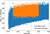 |
Fig. 1. Luminosity-redshift distribution for clusters in simulation of Seppi et al. (2022). Blue refers to the full population and orange to the one after the application of the ideal selection function. |
Mock observation selection function in terms of redshift and mass cuts.
3. Forward modeling
In this section, we detail the steps of our simulation pipeline that enabled us to generate galaxy cluster samples in terms of temperature, flux, and redshift distributions, based on input cosmology and the mass-luminosity scaling relation parameters. We assumed a flat ΛCDM model whereby the evolution of the scale factor is uniquely determined by Ωm and H0.
The adopted modeling scheme is summarized in Fig. 2. The pipeline incorporates our physical knowledge of cluster physics and the expected survey observables. Importantly, the approach described in this paper allowed us to easily adapt our pipeline to the observables at hand and integrate additional physical insights as needed. For instance, our procedure can be easily expanded to additional observables such as weak lensing shear (Tam et al. 2022) or richness.
 |
Fig. 2. Forward-modeling pipeline used to generate simulated samples of galaxy clusters from input parameters. We began with a set of input cosmological parameters: Ωm, σ8, and H0. From these parameters, we generated cluster masses within a fiducial volume slice of fixed redshift (see Section 3.1) using the HMF (see Section 3.2). Before applying the scaling relations, we ensured that the cluster masses were defined consistently with the cosmology associated with these relations (see Section 3.3). Luminosities and temperatures were then derived from these masses through scaling relations (see Section 3.4). We applied a k-correction to derive observer-frame luminosities (see Section 3.5) and used a β-model to rescale the predicted flux into a fixed physical aperture (see Section 3.6). Finally, we applied the selection function of the observed sample to the relevant observables to produce a mock catalog of galaxy clusters that is directly comparable with the observed sample (see Section 3.7). |
3.1. Survey volume
We started by calculating the survey volume in our input cosmology within redshift bins spanning the redshift range covered by the survey of interest. For the mock observation (Sect. 2), we defined redshift slices ranging from 0.1 to 0.6 in increments of 0.01. To ensure accurate modeling, the redshift bins were selected to be sufficiently fine, such that the mass function is assumed to be independent of redshift within each redshift slice. The binning strategy and the chosen redshift range can be easily adapted to any survey of interest. In this work, we considered two survey configurations with areas of 50 deg2 similar to the XMM-XXL survey (Pierre et al. 2016) and 1000 deg2 similar to Subaru/HSC-SSP survey (Aihara et al. 2018), enabling comparisons with surveys of varying sky coverage. The volume of each slice is calculated as
 (1)
(1)
where dV/dz is the differential comoving volume, which depends on cosmology, and dΩ is the survey area in steradians (Hogg 1999). We then generated clusters inside this fiducial volume by drawing objects from the mass function.
3.2. Mass function
Our redshift bins are chosen to be narrow enough such that the mass function is approximately independent of redshift within each slice. The mass function and its evolution are calculated at the mean redshift of each slice, using the colossus Python package Diemer (2018) and the Tinker et al. (2008) model. The Tinker et al. (2008) model was found to provide the closest representation of the HMF in the UNIT1i N-body simulation, which motivates our baseline choice. The effect of using a different mass function model, which would be less closely aligned with our mock data, is presented in Sect. 5.3.1. We generated halos within each redshift slice by drawing masses from the HMF within the mass range between 1.5 × 10¹⁴ M⊙ and 1015.5 M⊙ with a step size of 0.01 dex. Detecting a halo beyond these limits within our survey volume is highly improbable; thus, our choice allowed us to sample the entire mass range of interest. Masses were generated within an overdensity of Δc = 500. This choice arises from the definition of mass in the mass–temperature scaling relation (M-T), see Sect. 3.4.1, which is the typical overdensity within which weak-lensing (WL) masses are calculated. We define overdensity masses, MΔ, and radii, RΔ, as the mass and radius within which the mean density is Δc times the critical density of the Universe:
 (2)
(2)
with ρc(z) being the critical density of the Universe at the redshift of the system. The total number of halos within each redshift slice is given by the integral of the mass function over the mass and the survey volume:
 (3)
(3)
The approximation made in this equation follows from our assumption that the mass function does not evolve within the small redshift interval of any of our given bins.
The generated number of clusters within each redshift slice is given by a Poisson realization of the expectation value in Eq. (3). While the redshift of each slice is considered fixed for the purpose of mass generation using the HMF, the actual sources are distributed across a continuous range of redshifts. This was done by sampling from a distribution weighted by the differential comoving volume within each bin, allowing for a more realistic spread of source redshifts rather than assigning a single redshift to all sources in the slice.
3.3. Mass correction
The masses generated from the mass function are given within an overdensity of Δc = 500. Since ρc(z) = ρc, 0E(z) is cosmology dependent, with E(z) = H(z)/H0 being the expansion factor, the definition of MΔ is also cosmology dependent. To consistently apply scaling relations for galaxy clusters (see Sect. 3.4) and generate observables, we first had to convert our simulated masses into the cosmology assumed for these relations.
In our case, the mock catalog, and therefore the mass observable we used, were extracted from a simulation that assumed a Planck 2015 cosmology (Planck Collaboration XIII 2016). In the general case, we assumed that constraints on the M-T scaling relation are available in a fixed cosmology of choice, and within our pipeline we wished to convert the generated masses into the cosmology that was assumed to estimate the scaling relation.
Most recent estimates of the M-T scaling relation employ WL as a mass-calibration method (Mantz et al. 2016; Mulroy et al. 2019; Sereno et al. 2020), as the lensing signal is independent of a cluster’s dynamical state (Umetsu 2020). Therefore, we assumed that the relation between WL mass and gas temperature was previously calibrated in a fixed cosmology, and we used the background galaxy distribution to convert the simulated masses to the corresponding cosmology. We converted the mass calibration from one cosmology to another by taking into account the impact of the change in redshift–distance relation of the source’s lensed galaxies. Here, we assumed that our survey has properties similar to Subaru/HSC-SSP, leading to a redshift distribution that is similar to the one obtained in Umetsu et al. (2020).
In general, WL mass calibration employs either photo-z cuts or color–color cuts to identify foreground cluster and background galaxies (Medezinski et al. 2018). In this work, we adopted the photo-z cut approach of Umetsu et al. (2020), in which the photometric redshift probability distribution function (PDF), P(z), of each galaxy is used to select background sources behind a given cluster. Assuming a survey quality similar to HSC-SSP, we can estimate a realistic distribution of background galaxies as a function of cluster redshift. We assumed that the redshift distribution of background galaxies follows a known distribution, P(z). The cosmological dependence of the WL mass of the cluster inferred from these data can be described using the analytic formula introduced by Sereno (2015):
 (4)
(4)
where Ds and Dds represent the source and lens-source angular diameter distances, respectively. H(z) is the Hubble function evaluated at the redshift, z, of the cluster. Since the distance ratio between Ds and Dds varies for each background source, we computed the average of Eq. (4) over all background sources weighted by the number of background sources at each redshift, thus incorporating the stacked photo-z PDF ⟨P⟩(z) of the selected background galaxies behind the cluster:
 (5)
(5)
For each specific simulated cluster redshift in our pipeline, we searched for the cluster studied by Umetsu et al. (2020) with the closest redshift and associated the ⟨P⟩(z) distribution of the nearest neighbor to that cluster. Then, after calculating Eq. (5) for both our simulated cosmology and the cosmology within which the scaling relation was estimated, we obtained a mass-correction factor for the target cluster that is simply the ratio of these two quantities. This factor accounts for the cosmology-dependent change in the weak-lensing mass estimate, allowing us to transform the simulated mass into the equivalent lensing mass in the target cosmology. Assuming that the ⟨P⟩(z) distribution depends only on the redshift of our cluster, we computed the correction factor across a redshift grid ranging from 0.1 to 0.7 with a step of 0.05, and then interpolated for each generated redshift. We thus made the assumption that the depth of observations for WL is uniform across the survey, which is reasonable given the high homogeneity of the HSC-SSP survey depth (i ∼ 24.5 ABmag, Aihara et al. 2018). Finally, using the obtained correction factor, we converted our generated masses into the cosmology that was assumed for the estimation of the M-T relation, which we then used to generate mock observables.
3.4. Scaling relations
3.4.1. The mass–temperature scaling relation
In the self-similar model (Kaiser 1986) and its extensions (Ettori 2015; Ettori et al. 2020), ICM properties are expected to be tightly correlated with halo mass. In particular, the temperature is a tight proxy for the halo mass because of its dependency on the depth of the potential well (e.g., Nagai et al. 2007; Truong et al. 2018; Pop et al. 2022; Braspenning et al. 2024). In this work, we assumed that the M-T scaling relation is known, with an uncertainty and a scatter that we propagated into our simulation pipeline. In a more general case, our method can be adapted to the situation where WL studies are directly available, by jointly fitting the scaling relations and the cosmology.
Our mock observation was extracted from N-body simulations considering dark matter only, such that the gas properties had to be painted on using a semi-analytic approach (see Sect. 2). The semi-analytic model follows Comparat et al. (2020) to generate cluster properties from their mass, such as their temperature, T500, and luminosity, L500. We fit the M-T relation of the clusters in the mock catalog with a power law and found that the relation can be well described by
 (6)
(6)
with M500 and T500 being the mass and the temperature in an overdensity of 500, respectively. We therefore implemented this relation in our pipeline to generate temperatures from the simulated masses. Finally, the simulated temperatures are obtained as a Gaussian realization around the mean value, with a log-normal scatter of 0.07 dex that matches the scatter implemented in the Comparat et al. (2020) model. Both theoretical and observational studies have shown that this level of scatter is typical, as demonstrated, for example, by Truong et al. (2018).
3.4.2. The mass–luminosity scaling relation
The luminosity of a halo is linked to its gas fraction and, therefore, to its mass (e.g., Pratt et al. 2009). We modeled the mass-luminosity (M–L) scaling relation as a power law with a log-normal scatter:
 (7)
(7)
Here, Alm and Blm are the slope and the normalization of the relation, respectively. L500 represents the luminosity in the 0.5–2 keV energy band within an overdensity of 500. The 7/3 factor on E(z) arises from the definition of L500, which is the cylindrical luminosity integrated along the line of sight within a projected radius R500; see Lovisari & Maughan (2022) for more details.
While in principle the slope and normalization of the scaling relation can be predicted from the self-similar model, several studies found the M–L relation to be steeper than the self-similar expectation (Pacaud et al. 2007; Pratt et al. 2009; Bulbul et al. 2019; Lovisari et al. 2020). However, the relation can still be well described by a power law, as there is no evidence for a break in the relation down to group scales (Anderson et al. 2015; Zhang et al. 2024; Wood et al. 2025). Therefore, we treated the slope Alm, the normalization Blm, and the scatter σlm of the power law as free parameters in our pipeline to account for deviations from the self-similar model. As a result, the cosmological constraints we obtained will be marginalized over the uncertainty in the M-L relation, and the relation itself will be determined simultaneously with the cosmological parameters.
3.5. K-correction
The mass–luminosity relation defined in Eq. (7) is defined in the 0.5–2 keV band in the rest frame of each cluster, whereas the fluxes extracted from the survey were estimated in the corresponding band in the observer frame. Thus, a correction from rest frame to observer frame had to be applied for every simulated system, given its input redshift and temperature.
When going from the rest frame to the observer frame, the spectrum was shifted to lower energies due to the expansion of space between the source and the observer. Given the temperature of a simulated object, we used the Astrophysical Plasma Emission Code (APEC; Smith et al. 2001) model to calculate the flux ratio between the observed band and the band in the rest frame. We computed the flux in the observer frame accounting for redshift in the energy limits of the integral:
 (8)
(8)
Since this conversion does not depend on cosmology, we can define the quantity K as the ratio of the observed flux to the rest frame one, which is equivalent to the ratio of luminosities in the observer frame and rest frame. We assumed a constant gas metallicity of 0.3 Z⊙ with respect to the Asplund et al. (2009) solar-abundance table and a fixed absorption column density of NH = 1020 cm2, although in a general case the K-correction can easily be calculated as a function of NH. Given these assumptions, the conversion factor depends only on redshift and temperature. We calculated the conversion factor over a grid of redshifts and temperatures and interpolated over the grid to obtain the K factor of each generated cluster. The observed flux Fx is then obtained from the rest-frame luminosity as
 (9)
(9)
with K(T, z) being the K-correction at the temperature and redshift of each source and dL the luminosity distance.
3.6. Beta model and core radii
The luminosity we obtain from the M–L scaling relation is integrated within R500, which depends on the mass of the cluster. Given a model for the brightness distribution of the source, we can convert Fx, 500 into the flux estimated within a fixed physical aperture that is directly comparable to the measured fluxes. For a surface-brightness distribution, I(r), the flux integrated within a radius R becomes
 (10)
(10)
We modeled the brightness distribution of the simulated clusters using the beta model (Cavaliere & Fusco-Femiano 1976), which describes the expected emissivity distribution of an isothermal sphere in hydrostatic equilibrium:
 (11)
(11)
The shape of the distribution is governed by a single parameter, Rc, that is, the radius around which the profile transitions from a flat core to a power-law decrease. While clusters generally deviate from isothermal spheres, the beta model is known to provide a good approximation of the brightness distribution, with deviations at the level of ∼10% (Käfer et al. 2019). Given values of R500 and Fx, 500, we were able to obtain the normalization of the beta model, I0, and thus a flux within any aperture. Studies of the brightness distribution in galaxy clusters showed that the β parameter is usually around 2/3 (e.g., Mohr et al. 1999; Chen et al. 2007; Eckert et al. 2011; Käfer et al. 2019). Assuming β = 2/3, the flux enclosed within radius R thus becomes
![Mathematical equation: $$ \begin{aligned} F( < R) = 2\pi I_0 R_c^2\left[1-\left(1+ \left(R/R_c\right)^2\right)^{-1/2} \right] .\end{aligned} $$](/articles/aa/full_html/2026/04/aa55835-25/aa55835-25-eq13.gif) (12)
(12)
To account for realistic structural variations among the cluster population, we simulated the core radius based on the distribution of values observed in well-studied clusters; see Appendix B for a full description of the procedure. Käfer et al. (2019) demonstrated that the luminosities and core radii of clusters are anticorrelated, which can be explained by the dependence of the surface-brightness profile on the dynamical state (e.g., Leccardi et al. 2010; Rossetti et al. 2017; Andrade-Santos et al. 2017). We injected this knowledge into our pipeline by simultaneously generating the scatter in the luminosities and the core radii from a multivariate Gaussian distribution, assuming a correlation coefficient of −0.43 between Rc and L500 (Käfer et al. 2019).
In practice, the mass of each system is not known a priori, and the fluxes within R500 cannot be easily estimated observationally. Therefore, we assume that the fluxes were extracted within fixed physical apertures. The choice of the aperture is arbitrary, but fixed and known in advance. Here, following Giles et al. (2016), we assumed an aperture of 300 kpc, which should encompass the majority of the flux for the objects we deteced. We stress that our method can work for any choice of aperture as long as it is treated consistently, meaning that we can adapt our simulated aperture to any observed survey. From the luminosity, the core radius, and the beta model, we can easily and analytically calculate a flux within any aperture and inject it into the simulation pipeline to replicate a fixed aperture in a fixed cosmology.
3.7. Selection function
To ensure that our simulations are comparable to the data, the selection function of the survey needed to be implemented. With our approach, we can generate observables as they are used for the selection function of a survey. Our methodology enabled us to generate these parameters directly, ensuring that the selection function was accurately applied and that the sample we produced closely mirrors what would be observed by the survey. In the case of the mock observation used in this study and described in Sect. 2, the selection function is simply a cut in mass, M500c > 1014.2 M⊙, and redshift 0.1 < z < 0.6. However, we stress that the approach proposed here allowed us to implement any selection function in an exact way, provided that the selection is sufficiently understood.
3.8. Posterior estimation with SBI
With the forward-modeling pipeline in hand, a likelihood-free inference scheme was required to compare the simulated samples with the observational dataset and estimate the posterior distributions of the model parameters. We used the sbi Python package (Tejero-Cantero et al. 2020; Boelts et al. 2025). The code generates a large number of simulations, spanning a predefined range of parameter values, allowing us to vary different input parameters of a specifically defined model. We then used the sequential neural posterior estimation (SNPE; Greenberg et al. 2019) method to learn the mapping between the input parameters and the simulated samples and return posterior distributions of each parameter using the masked autoregressive flow (MAF) neural density estimator (Papamakarios et al. 2017) provided by sbi. In our implementation, we used the default network architecture of sbi (version 0.23.3), these defaults may change in future versions. SNPE is particularly efficient for exploring the parameter space when simulations are computationally expensive, although it sacrifices amortization, meaning that the network must be retrained for each new observation. The neural density estimator is trained to approximate the posterior distribution of parameters given the simulated data by minimizing the Kullback–Leibler (KL) divergence. In our implementation, the final posterior was obtained from this single trained neural density estimator. Once the model was trained, we applied it to the observed dataset and sampled the parameters directly from the learned posterior distribution, which is represented by a neural density estimator. We applied flat priors to the parameters of interest (see Table 2) and generated 10 000 simulations using parameters drawn from the prior distribution.
Priors used for each input parameter of the pipeline in the SBI optimization algorithm.
To ensure consistent input for the neural density estimator, both the observed dataset and simulated outputs were transformed into fixed-size histograms of temperature, flux, and redshift (see Table 3 and Fig. 3), which were then combined into a single data vector.
 |
Fig. 3. Temperature, flux, and redshift histograms for 1000 deg2 with the UNIT1i mock observation in red and results computed from the obtained posterior parameters in blue. The blue points show the median value for each bin across a range of simulated samples generated from the posterior distributions using our method with flat priors for each parameter and a uniform proposal distribution for training the model. The error bars show the standard deviation of the simulated samples in each bin. |
Bins used to create output temperature, flux, and redshift histograms in the SBI optimization algorithm.
We tested several different configurations for the definition of the data vector, including a 3D histogram of flux, temperature, and redshift, and a 2D histogram for the flux and temperature with a separate 1D histogram for the redshift distribution. We find that the 2D solution is more stable; thus, for the remainder of the paper we adopt this configuration. For more details on the different setups, we refer the reader to Appendix H.
To train the model in SBI, the parameter space was explored by randomly sampling values from the prior distribution. In this case, we used the priors outlined in Table 2, which specify plausible ranges for each of the parameters of interest, meaning the parameter space has been uniformly explored across the 6D cube set by the individual prior ranges. Uniform sampling ensures a broad exploration of all possible solutions, without biasing the search in favor any specific region.
To improve efficiency and reduce time spent exploring uninformative regions of the parameter space, we tried to enhance the sampling strategy by introducing a nonuniform proposal distribution. To do so, we first trained a model on a sample generated from a uniform proposal and inferred a posterior distribution. From the resulting posterior, we drew 100 000 samples, which were then used to compute a Fisher matrix. This matrix defined a multivariate normal distribution that served as our updated proposal. Additional configuration details and results are provided in Appendix G.
4. Results
In this section, we present the results of our tests evaluating the performance of our method and the SBI approach. Since the cosmological parameters used to generate the UNIT1i mock observation are known (see Table 4), we tested the ability of our method to recover these parameters.
Definition of six pipeline parameters, their mock UNIT1i values (true values), and their inferred values obtained through SBI.
4.1. Validation of SBI-inferred Parameters
We tested the performance of the SBI method applied to our pipeline through its ability to reproduce the observed distributions of temperature, flux, and redshift. To achieve this, we selected a region of 1000 deg2 from the half-sky light cone and attempted to recover the input parameters using the model trained with uniform proposals on each parameter corresponding to the chosen prior ranges (see Table 2). To verify that the model provides an adequate representation of the data, we then randomly selected 1000 parameter sets from the posterior distribution and generated a simulated sample for each using our pipeline. The median and dispersion of the resulting samples were then computed in each redshift, temperature, and flux bin. Fig. 3 shows how these distributions compare with those of the mock observation.
This comparison clearly demonstrates that, with flat priors and a uniform proposal over 1000 deg2, our method effectively converges to parameters that replicate the temperature, flux, and redshift distributions extracted from the mock observation. However, small deviations between the simulated samples and the data can be observed, particularly at redshifts of z > 0.4; the following section investigates the quality of the fit to determine whether these discrepancies are consistent with statistical fluctuations or indicative of a systematic effect.
4.2. Goodness of fit
A key question in our analysis is whether the observed data are compatible with a random realization of our simulation pipeline from the posterior distributions. In other words, we sought to determine whether it is plausible that the available data correspond to an expected outcome generated by our forward simulation framework. To this end, we drew 1000 parameter sets from the posterior distributions and generated mock data vectors using our simulation pipeline in a fiducial area of 1000 deg2.
Since we did not have access to an analytical likelihood, a traditional goodness-of-fit test could not be performed to evaluate the efficiency of our trained model. However, to retain this evaluation metric, we implemented a modified version of the χ2 goodness-of-fit test following the approach presented in von Wietersheim-Kramsta et al. (2025). Namely, we introduced a test statistic, C, as the Poissonian log-likelihood of the observed data points with respect to the mean of the 1000 simulated samples:
 (13)
(13)
where Λ(μ, k) represents the Poisson probability distribution in each bin, with μ being the mean of all realizations and k the value of a specific realization. In the Gaussian case, C naturally translates into the standard χ2 formula, making it a direct generalization of the traditional χ2 test to the case of Poisson-distributed data.
Figure 4 shows the cumulative distribution function (CDF) of C values obtained from the 1000 realizations in blue, along with the C value corresponding to the mock data, shown as a red dashed line. This comparison allows us to assess the coverage of the posterior distributions of parameters with respect to the true value. We can see that the test statistic value obtained for the data corresponds to a CDF value of 0.51, such that 49% of the randomly generated samples exhibit a value of the test statistic that is larger than the value obtained for the mock observation. Nevertheless, turning this result into a null hypothesis probability is not straightforward. We chose this approach because, for real observations, the true parameter values are unknown. Since in our case we tested the model on mock observations with known true parameters, we additionally performed 1000 realizations by fixing the input parameters to the Planck cosmology and to the fit scaling relation parameters of the mock observation; see UNIT1i value in Table 4. This test reveals that the measured test statistic values lie on the upper end of the distribution expected from the true parameters. This was expected, as our pipeline includes a number of simplifications and neglects some effects present in the mock, which was extracted from a full N-body simulation. We found that cosmic variance and uncertainties in the HMF are the most important systematic uncertainties in our modeling. We consider the impact of these residual systematics in Sect. 5.3, with their relative impact on each inferred parameter listed in Table 4. Comparing the fit parameters to the input values, we can see that varying the scaling relation parameters makes it possible to absorb these systematic differences without biasing the retrieved cosmological parameters.
 |
Fig. 4. Cumulative distribution of test statistic C obtained from 1000 realizations coming from random points in the parameter posterior distributions for the 1000 deg2 test. The dashed red line is the C value of the mock observation. |
4.3. Posterior distributions
The corner plot shown in Fig. 5 displays the posterior distributions of the parameters within our pipeline. It includes three cosmological parameters (Ωm, σ8, and H0) and three parameters related to the M-L scaling relation (slope, normalization, and log-normal intrinsic scatter).
 |
Fig. 5. Corner plot of six posterior distributions corresponding to each parameter of the pipeline: the three cosmological parameters Ωm, σ8, and H0; and the three parameters from the M–L scaling relation Alm, Blm, and σlm corresponding to the slope, the normalization, and the scatter, respectively. The results correspond to a run with flat priors on each parameter (see Table 2) and a uniform proposal for the training of the model, on a fiducial area of 1000 deg2. The contours represent the 1σ and 2σ confidence levels, and the dashed red lines are the UNIT1i values. |
In Table 4, we present the best-fitting values obtained with our pipeline along with their corresponding statistical and systematic errors, which are discussed in Sect. 5.3. We compared them to the input cosmological parameters used to generate the UNIT1i light cone, as well as to the M–L relation parameters that were fit directly from the mock catalog. While the cosmological parameters were explicitly set in the simulation, the M–L parameters were not defined a priori, since the mock does not rely on scaling relations to assign luminosities. Instead, we derived them by fitting the mock cluster masses and luminosities. We can see that the retrieved parameters are fully consistent with the input values, which confirms the effectiveness of our approach. The corner plot highlights the known degeneracy between Ωm and σ8. We also note that Ωm and σ8 appear to be correlated with H0. The observed degeneracy between H0 and Ωm arises from their combined influence on the predicted number of galaxy clusters. While H0 significantly impacts the comoving volume (see Eq. 1), Ωm governs the shape and normalization of the halo mass function, which dictates the number density of massive objects. As a result, a higher H0, which reduces the survey volume, can be compensated by a higher Ωm to maintain the same number of detected clusters, and vice versa. This volume–mass function trade-off generates the observed degeneracy. Furthermore, the correlation between H0 and σ8 is indirectly driven by their respective degeneracies with Ωm. Appendix D shows that this effect is not visible in smaller survey areas (e.g., 50 deg2), but becomes significant for larger samples such as the 1000 deg2 case studied here.
A clear correlation is observed between the slope and normalization of the luminosity–mass (M–L) scaling relation, Alm and Blm, respectively. We note that the degeneracy between the slope and the normalization of the luminosity–mass relation arises from our choice of pivot point (1014 M⊙, see Eq. 7), which is located below the limiting mass considered in the mock analysis. The degeneracy would disappear if the pivot point was set at a slightly higher mass or if the sample extended to lower masses, as is the case, for example, of the XMM-XXL (Pierre et al. 2016) and eROSITA/eRASS1 (Ghirardini et al. 2024) samples.
4.4. Coverage test
To assess the coverage properties of our trained model, we performed a dedicated test aimed at verifying whether the inferred posteriors are statistically consistent with the true parameters. This test is computationally intensive, so we carried it out on the 50 deg2 configuration. We began by generating catalogs of clusters in a 50 deg2 area, from 10 000 random points in the prior parameter space. For each generated catalog, we applied the model trained on the same survey area and drew 10 000 samples using the sbi framework. From the resulting posterior chains, we then randomly selected one point per parameter.
Figure 6 compares the input values (true value) to the inferred ones for the six parameters of the simulation pipeline. We visualize the results using a Gaussian kernel density estimator and indicate the median of the points with a dashed red line. To minimize the impact of prior boundaries on the inferred parameters, which could bias the results if we adopt the median of the posterior as our point estimate, we instead selected a random point from the posterior chain. Nevertheless, we still note a slight overestimation and underestimation of the recovered points close to the lower and upper boundaries of the prior, respectively. This behavior is expected, as the shape of the prior in these regions is highly asymmetric. This implies that the posterior distributions are highly skewed and the median of the posterior is biased.
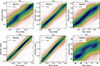 |
Fig. 6. Results of coverage test described in Sect. 4.4, comparing the input values (true values) to the inferred ones for each parameter by taking random points in the posterior distribution chains. The point density was smoothed using a Gaussian kernel-density estimator and indicated by the color code, with the median of the points indicated by a dashed red line, and the 1:1 line in black. |
We first note that our model effectively constrained the σ8 parameter, as evidenced by the high density of points around the 1:1 line. As for Ωm, the method recovered it in an unbiased manner, with a clear concentration of points around the 1:1 line. However, while the recovery of Ωm is accurate, the precision is lower compared to σ8, as shown by the larger scatter around the 1:1 line.
Regarding the scaling relation parameters, they are all well constrained, suggesting that our model can constrain the cosmological parameters and the M–L scaling relation simultaneously. While the model precisely constrained the normalization of the M–L relation, the slope was not as well constrained, with the scatter of the points around the 1:1 line showing a larger uncertainty around the true value. This is due to the mass cut imposed by the selection function, which reduces sensitivity to the slope, given the absence of low-mass clusters in the selected sample.
For a 50 deg2 survey, H0 is poorly constrained, as the point density is not concentrated around the 1:1 line. Since the cluster count method is not highly sensitive to H0, this outcome is expected. By treating H0 as a free parameter in our simulation pipeline, we marginalized over its uncertainty when constraining the other parameters. Nonetheless, some sensitivity to H0 remains, as the posterior distribution is not completely flat for a 50 deg2 survey. Larger surveys are more sensitive to H0, as demonstrated in the 1000 deg2 case shown in Fig. 5 and Appendix D.
5. Discussion
5.1. Comparison with traditional methods
Traditional analyses of galaxy cluster counts typically rely on analytic likelihoods and simplified assumptions about the survey selection function and scaling relations. However, such approaches are often unable to marginalize over important systematics, including uncertainties in the observable–mass relation, approximations in the mass function, and incomplete modeling of the selection effects. In contrast, the SBI method used in this work provides a robust alternative by forward modeling the entire observed cluster population. It fits directly to the observables, without requiring an explicit likelihood. The simulation process naturally accounts for all cosmological dependencies. Crucially, it enables a more accurate treatment of complex effects such as the survey selection function, the intrinsic scatter and covariance in scaling relations, and selection biases linked to profile shapes or morphological properties. It also allows us to marginalize over modeling uncertainties by directly sampling uncertain physical parameters over their allowed range. As a result, it offers a more flexible and potentially more accurate framework for extracting cosmological information from cluster surveys.
Another key advantage of the SBI approach is its ability to integrate multiple datasets into a single pipeline, enabling joint analyses across observables such as clustering, cluster counts, and baryon acoustic oscillations (BAO). While traditional methods can also combine such datasets, SBI can account for the covariance between observables through the forward modeling process, provided that the relevant physical processes are included in the simulation pipeline. By predicting multiple observables from the same cosmological model, this approach allowed us to enrich the model by adding more data to the observable vector, making the analysis more powerful and flexible. With our framework, it is relatively straightforward to include other cosmological probes to improve the constraints and provide a self-consistent inference across all probes. However, compatibility between probes is not guaranteed, as each may have its own systematic uncertainties. A prudent strategy is to test each probe independently and compare the results. This can reveal potential tensions, opening the door to further investigation. Ultimately, combining probes coherently can yield more robust constraints and a deeper understanding of the cosmological model.
5.2. Survey size
We investigated the impact of the survey size on the uncertainty of the inferred parameters. To do so, we compared the results obtained from a mock survey covering 50 deg2 with those from a mock survey covering 1000 deg2, focusing on the joint posterior distributions of Ωm and σ8; see Fig. 7. In both cases, the parameter estimates converge to values consistent with the Planck results (Planck Collaboration XIII 2016) within 1σ, confirming that the model reliably recovers cosmological parameters. As expected, increasing the survey size significantly reduces the uncertainties on each parameter, highlighting the advantage of larger datasets in improving parameter constraints. As a step in this direction, we conducted a mock analysis with the same number of clusters as eRASS1 to explore its potential application; see Appendix I.
 |
Fig. 7. Posterior distributions in Ωm − σ8 plane for mock survey areas of 50 deg2 in blue and 1000 deg2 in orange, compared to the Planck values used in UNIT1i in green. The contours represent the 1σ and 2σ confidence levels. |
5.3. Systematic uncertainties
We analyzed the impact of systematic errors in our method and how they affect the results. Specifically, we considered three key sources of systematics: the choice of the mass function, the normalization of the M–T relation, and sample variance. Variations in the mass function can lead to differences in the inferred cosmological parameters, while uncertainties in the M–T normalization directly influenced mass estimates and, consequently, constraints on σ8 and Ωm. Finally, sample variance, inherent to the limited survey area, introduced additional fluctuations that had to be taken into account in our analysis. Although these systematic effects are subdominant compared to the statistical uncertainties, their combined contribution is reported in Table 4. This combined systematic uncertainty was obtained as the quadrature sum of the three sources of systematic error, scaled to a 1000 deg° survey. To obtain the total uncertainty on each parameter, the statistical and systematic components should be added in quadrature.
5.3.1. Mass-function-model comparison
For the galaxy cluster count approach, the choice of the mass function introduces a systematic uncertainty. To investigate the impact of the choice of mass function on the recovered cosmological parameters, we compared four different mass-function models implemented in the colossus Python package: Watson13 (Watson et al. 2013), Despali16 (Despali et al. 2016), Tinker08 (Tinker et al. 2008), and Bocquet16 (Bocquet et al. 2016). The first three were calibrated using dark-matter-only N-body simulations, whereas Bocquet16 is based on hydrodynamical simulations that incorporate baryonic physics.
In the left panel of Fig. 8, we plot the four mass-function models evaluated at the median redshift of the mock observation (z = 0.426) and display the ratio of the various models to our default model (Tinker08). In the mass range covered by our data, the Tinker08, Despali16, and Bocquet16 models are consistent with one another at the ∼20% level, whereas the Watson13 model deviates by more than 50%. Large differences between the models can be observed at very high masses (> 1015 M⊙). However, such massive clusters are very rare and mostly absent within an area of 50 deg2. In the right panel of Fig. 8, we show the values of Ωm and σ8 recovered with our pipeline over a 50 deg2 area for the four different mass functions. The systematic uncertainty induced by the choice of the mass function is not particularly problematic over this survey size, similarly to the XMM–XXL field. We adopted the Tinker08 model by default as it was found to provide the best match to the intrinsic UNIT1i mass function (Seppi et al. 2022). The largest deviations compared to the default Tinker08 model reach up to ∼16% for Ωm and ∼4% for σ8, with the Watson13 model showing both the largest offset and a noticeably different degeneracy direction between Ωm and σ8, which is due to the different slope of the HMF in the 1014 − 1015 M⊙ range compared to the other models.
 |
Fig. 8. Left panel shows a comparison of mass function models available in the colossus Python package relative to the Tinker08 model, in the cosmology of the mock observation; i.e., Ωm = 0.3089, σ8 = 0.8159, and H0 = 67.74, and for z = 0.426, which is the median redshift of the mock observation. The bottom plot shows the residuals. The right panel shows the crossed posterior distributions of Ωm and σ8 for a mock survey covering 50 deg2 with a nonuniform proposal. Different colors represent different runs, each using a distinct mass function model available in the colossus Python package. The Planck value of Ωm and σ8, which corresponds to the true values implemented in the mock, is also shown for reference. The contours represent the 1σ and 2σ confidence levels. |
This effect is expected to be more relevant for larger fields such as eROSITA. For a 50 deg2 area, the statistical uncertainties dominate and mask the systematic differences due to the choice of mass function. While the systematic uncertainty from the mass function will eventually become dominant as survey size increases, it remains subdominant compared to statistical errors at the scale of our current analysis. In other words, as survey areas grow and statistical uncertainties shrink, the choice of mass function will play an increasingly important role in the error budget.
5.3.2. Sample variance
We investigated the impact of sample variance by retrieving the cosmological parameters from five different areas extracted from the UNIT1i light cone, each covering 50 deg2 (see the left panel of Fig. 9). This sample variance, which arises from the large-scale structure and represents a source of error not accounted for in our simulation pipeline, could potentially affect our results. However, the differences observed between the various tested regions are smaller than the associated error bars. Therefore, we can reasonably conclude that the sample variance does not significantly impact the results for the 50 deg2 areas and can be considered negligible in this context. Sample variance decreases with survey size and is thus not expected to play an important role for wider surveys.
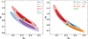 |
Fig. 9. Left panel shows a sample variance test in the form of 2D posterior distributions of Ωm and σ8 for different 50 deg2 regions of the mock observation with a uniform proposal. The contours represent the 1σ and 2σ confidence levels. The right panel is the crossed posterior distributions of Ωm and σ8 for a mock survey covering an area of 50 deg2 with a uniform proposal. The distribution shown in blue assumes an M–T normalization parameter of 2.104 (see 3.4.1), while the distributions in orange and red correspond to variations of plus and minus 10% around this value, respectively. The results are compared with the Planck values used in UNIT1i (represented in green). The contours indicate the 1σ and 2σ confidence intervals. |
5.3.3. Mass–temperature normalization
The information on the mass scale in our simulation pipeline is encoded within the normalization of the M-T relation, which we set using external constraints. The M-T normalization parameter is fixed at 2.104 keV at the pivot mass of 1014 M⊙ (see Section 3.4.1), a value calibrated from WL measurements that carries an estimated uncertainty of about 10%. This external uncertainty could potentially introduce a systematic bias on the resulting cosmological parameters. To assess the impact of the mass calibration, we tested how varying this parameter by ±10% affects our results. The right panel of Fig. 9 shows the posterior distributions in the Ωm − σ8 plane when changing the normalization of the M–T relation by ±10%, over an area of 50 deg2. We repeated the analysis over the same five regions as for the sample variance (see Section 5.3.2) and display a single one as a representative example here. Similar trends can be seen in all five mock areas we tested. We can see that the contours shift as a function of the M–T normalization. When the M-T normalization increases by 10%, Ωm goes up by 17% with a median value of 0.384, while σ8 drops by 5% with a median value of 0.736. On the other hand, decreasing the M-T normalization by 10% leads to a 28% drop in Ωm with a median value of 0.238, and an 11% increase in σ8 with a median value of 0.861. Interestingly, we observe that while both Ωm and σ8 change significantly, the quantity S8 = σ8(Ωm/0.3)0.3 remains almost unchanged, varying by only 4%. Indeed, the contours move along the well-known degeneracy between these parameters, such that the value of S8 remains almost unchanged. Therefore, our analysis shows that the value of S8 inferred with our method is robust against uncertainties in the absolute mass calibration. The retrieved values of Ωm, σ8, and S8 over the five separate 50 deg2 are provided in Appendix E.
6. Conclusion
In this work, we demonstrated the effectiveness of SBI as a powerful method for cosmological analysis. This approach enables us to forward fit observables directly, incorporating all cosmological dependencies naturally into the simulation pipeline. Generating observables directly allows for the precise application of the selection function within the parameter space where it is defined, ensuring robust and accurate results. Additionally, the implementation of a covariance matrix as a proposal during the training phase of the model significantly accelerates convergence, making the method more efficient and well-suited to this type of problem.
To validate our method, we used mock cluster samples extracted from the UNIT1i dark-matter halo simulation. The N-body halos were assigned X-ray properties (temperature and luminosity) using a semi-analytic approach (Comparat et al. 2020), and mock catalogs were generated from the resulting light cone over areas of 50 deg2 and 1000 deg2. We first applied our method to the 1000 deg2 mock observation and confirmed that the method performs as expected when comparing the retrieved cosmological parameters with the values that were used to generate the N-body simulation. Additionally, we verified that increasing the survey size significantly improves the precision of parameter estimates, highlighting the potential of this approach for future large-area surveys.
Furthermore, we assessed the impact of systematic errors related to sample variance and the choice of the mass function model. We found that for an area of 50 deg2, these systematic uncertainties are subdominant, further validating the robustness of the method for this scale. However, these systematic uncertainties can become substantial in cluster-count experiments covering wider areas, such as eROSITA (Ghirardini et al. 2024) or Euclid (Euclid Collaboration: Bhargava et al. 2026).
One key factor that significantly improves the precision of the σ8 parameter is the inclusion of information on the temperature distribution. Since the temperature acts as an effective proxy for the halo mass, it provides tighter constraints on the mass distribution, which in turn enhances our ability to accurately infer σ8. This demonstrates the importance of low-scatter mass proxies for more precise cosmological parameter estimates.
Acknowledgments
We thank Benjamin Joachimi, Michael Burgess, Ben Maughan, and Sebastian Grandis for useful discussions that lead to significant improvements in the paper. MR, DE, and RS acknowledge support from the Swiss National Science Foundation (SNSF) through grant agreement #200021_212576. K.U. acknowledges support from the National Science and Technology Council, Taiwan (grant NSTC 112-2112-M-001-027-MY3) and the Academia Sinica Investigator award (grant AS-IA-112-M04).
References
- Abdalla, E., Abellán, G. F., Aboubrahim, A., et al. 2022, J. High Energy Astrophys., 34, 49 [NASA ADS] [CrossRef] [Google Scholar]
- Adami, C., Giles, P., Koulouridis, E., et al. 2018, A&A, 620, A5 [NASA ADS] [CrossRef] [EDP Sciences] [Google Scholar]
- Aihara, H., Armstrong, R., Bickerton, S., et al. 2018, PASJ, 70, S8 [NASA ADS] [Google Scholar]
- Allen, S. W., Evrard, A. E., & Mantz, A. B. 2011, ARA&A, 49, 409 [Google Scholar]
- Anderson, M. E., Gaspari, M., White, S. D. M., Wang, W., & Dai, X. 2015, MNRAS, 449, 3806 [NASA ADS] [CrossRef] [Google Scholar]
- Andrade-Santos, F., Jones, C., Forman, W. R., et al. 2017, ApJ, 843, 76 [Google Scholar]
- Asgari, M., Lin, C.-A., Joachimi, B., et al. 2021, A&A, 645, A104 [NASA ADS] [CrossRef] [EDP Sciences] [Google Scholar]
- Asplund, M., Grevesse, N., Sauval, A. J., & Scott, P. 2009, ARA&A, 47, 481 [NASA ADS] [CrossRef] [Google Scholar]
- Bocquet, S., Saro, A., Dolag, K., & Mohr, J. J. 2016, MNRAS, 456, 2361 [Google Scholar]
- Bocquet, S., Dietrich, J. P., Schrabback, T., et al. 2019, ApJ, 878, 55 [Google Scholar]
- Boelts, J., Deistler, M., Gloeckler, M., et al. 2025, J. Open Source Software, 10, 7754 [Google Scholar]
- Braspenning, J., Schaye, J., Schaller, M., et al. 2024, MNRAS, 533, 2656 [NASA ADS] [CrossRef] [Google Scholar]
- Bulbul, E., Chiu, I. N., Mohr, J. J., et al. 2019, ApJ, 871, 50 [Google Scholar]
- Cavaliere, A., & Fusco-Femiano, R. 1976, A&A, 49, 137 [NASA ADS] [Google Scholar]
- Chen, Y., Reiprich, T. H., Böhringer, H., Ikebe, Y., & Zhang, Y. Y. 2007, A&A, 466, 805 [NASA ADS] [CrossRef] [EDP Sciences] [Google Scholar]
- Chiu, I. N., Klein, M., Mohr, J., & Bocquet, S. 2023, MNRAS, 522, 1601 [NASA ADS] [CrossRef] [Google Scholar]
- Chuang, C.-H., Yepes, G., Kitaura, F.-S., et al. 2019, MNRAS, 487, 48 [NASA ADS] [CrossRef] [Google Scholar]
- Clerc, N., & Finoguenov, A. 2023, in Handbook of X-ray and Gamma-ray Astrophysics, 123 [Google Scholar]
- Clerc, N., Pierre, M., Pacaud, F., & Sadibekova, T. 2012, MNRAS, 423, 3545 [NASA ADS] [CrossRef] [Google Scholar]
- Comparat, J., Eckert, D., Finoguenov, A., et al. 2020, Open J. Astrophys., 3, 13 [Google Scholar]
- Despali, G., Giocoli, C., Angulo, R. E., et al. 2016, MNRAS, 456, 2486 [NASA ADS] [CrossRef] [Google Scholar]
- Di Valentino, E., Said, J. L., Riess, A., et al. 2025, Phys. Dark Univ., 49, 101965 [Google Scholar]
- Diemer, B. 2018, ApJS, 239, 35 [NASA ADS] [CrossRef] [Google Scholar]
- Dodelson, S., Heitmann, K., Hirata, C., et al. 2016, arXiv e-prints [arXiv:1604.07626] [Google Scholar]
- Eckert, D., Molendi, S., & Paltani, S. 2011, A&A, 526, A79 [NASA ADS] [CrossRef] [EDP Sciences] [Google Scholar]
- Eckert, D., Ghirardini, V., Ettori, S., et al. 2019, A&A, 621, A40 [NASA ADS] [CrossRef] [EDP Sciences] [Google Scholar]
- Ettori, S. 2015, MNRAS, 446, 2629 [NASA ADS] [CrossRef] [Google Scholar]
- Ettori, S., Lovisari, L., & Sereno, M. 2020, A&A, 644, A111 [EDP Sciences] [Google Scholar]
- Euclid Collaboration (Bhargava, S., et al.) 2026, A&A, in press, https://doi.org/10.1051/0004-6361/202554937 [Google Scholar]
- Finoguenov, A., Rykoff, E., Clerc, N., et al. 2020, A&A, 638, A114 [NASA ADS] [CrossRef] [EDP Sciences] [Google Scholar]
- Garrel, C., Pierre, M., Valageas, P., et al. 2022, A&A, 663, A3 [NASA ADS] [CrossRef] [EDP Sciences] [Google Scholar]
- Ghirardini, V., Bulbul, E., Artis, E., et al. 2024, A&A, 689, A298 [NASA ADS] [CrossRef] [EDP Sciences] [Google Scholar]
- Giles, P. A., Maughan, B. J., Pacaud, F., et al. 2016, A&A, 592, A3 [NASA ADS] [CrossRef] [EDP Sciences] [Google Scholar]
- Giodini, S., Lovisari, L., Pointecouteau, E., et al. 2013, Space Sci. Rev., 177, 247 [Google Scholar]
- Grandis, S., Bocquet, S., Mohr, J. J., Klein, M., & Dolag, K. 2021, MNRAS, 507, 5671 [NASA ADS] [CrossRef] [Google Scholar]
- Greenberg, D. S., Nonnenmacher, M., & Macke, J. H. 2019, Automatic Posterior Transformation for Likelihood-Free Inference [Google Scholar]
- Haiman, Z., Mohr, J. J., & Holder, G. P. 2001, ApJ, 553, 545 [NASA ADS] [CrossRef] [Google Scholar]
- Hi4PI Collaboration (Ben Bekhti, N., et al.) 2016, VizieR On-line Data Catalog: J/A+A/594/A116 [Google Scholar]
- Hogg, D. W. 1999, arXiv e-prints [arXiv:astro-ph/9905116] [Google Scholar]
- Käfer, F., Finoguenov, A., Eckert, D., et al. 2019, A&A, 628, A43 [Google Scholar]
- Kaiser, N. 1986, MNRAS, 222, 323 [Google Scholar]
- Kosiba, M., Cerardi, N., Pierre, M., et al. 2025, A&A, 693, A46 [NASA ADS] [CrossRef] [EDP Sciences] [Google Scholar]
- Leccardi, A., Rossetti, M., & Molendi, S. 2010, A&A, 510, A82 [NASA ADS] [CrossRef] [EDP Sciences] [Google Scholar]
- Liu, A., Bulbul, E., Ghirardini, V., et al. 2022, A&A, 661, A2 [NASA ADS] [CrossRef] [EDP Sciences] [Google Scholar]
- Lovisari, L., & Maughan, B. J. 2022, in Handbook of X-ray and Gamma-ray Astrophysics, eds. C. Bambi, & A. Sangangelo, 65 [Google Scholar]
- Lovisari, L., Reiprich, T. H., & Schellenberger, G. 2015, A&A, 573, A118 [NASA ADS] [CrossRef] [EDP Sciences] [Google Scholar]
- Lovisari, L., Schellenberger, G., Sereno, M., et al. 2020, ApJ, 892, 102 [Google Scholar]
- Lovisari, L., Ettori, S., Gaspari, M., & Giles, P. A. 2021, Universe, 7, 139 [NASA ADS] [CrossRef] [Google Scholar]
- Mantz, A., Allen, S. W., Ebeling, H., Rapetti, D., & Drlica-Wagner, A. 2010a, MNRAS, 406, 1773 [NASA ADS] [Google Scholar]
- Mantz, A., Allen, S. W., Rapetti, D., Ebeling, H., & Drlica-Wagner, A. 2010b, Am. Astron. Soc. Meeting Abstr., 215, 437.10 [Google Scholar]
- Mantz, A. B., Allen, S. W., Morris, R. G., et al. 2015a, MNRAS, 449, 199 [CrossRef] [Google Scholar]
- Mantz, A. B., von der Linden, A., Allen, S. W., et al. 2015b, MNRAS, 446, 2205 [Google Scholar]
- Mantz, A. B., Allen, S. W., Morris, R. G., & Schmidt, R. W. 2016, MNRAS, 456, 4020 [NASA ADS] [CrossRef] [Google Scholar]
- Maughan, B. J. 2007, ApJ, 668, 772 [Google Scholar]
- Maughan, B. 2012, in Galaxy Clusters as Giant Cosmic Laboratories, ed. J.-U. Ness, 36 [Google Scholar]
- Maughan, B. J., Giles, P. A., Randall, S. W., Jones, C., & Forman, W. R. 2012, MNRAS, 421, 1583 [Google Scholar]
- Medezinski, E., Oguri, M., Nishizawa, A. J., et al. 2018, PASJ, 70, 30 [NASA ADS] [Google Scholar]
- Mohr, J. J., Mathiesen, B., & Evrard, A. E. 1999, ApJ, 517, 627 [Google Scholar]
- Mulroy, S. L., Farahi, A., Evrard, A. E., et al. 2019, MNRAS, 484, 60 [NASA ADS] [CrossRef] [Google Scholar]
- Nagai, D., Kravtsov, A. V., & Vikhlinin, A. 2007, ApJ, 668, 1 [Google Scholar]
- Pacaud, F., Pierre, M., Refregier, A., et al. 2006, MNRAS, 372, 578 [NASA ADS] [CrossRef] [Google Scholar]
- Pacaud, F., Pierre, M., Adami, C., et al. 2007, MNRAS, 382, 1289 [Google Scholar]
- Pacaud, F., Pierre, M., Melin, J. B., et al. 2018, A&A, 620, A10 [NASA ADS] [CrossRef] [EDP Sciences] [Google Scholar]
- Papamakarios, G., Pavlakou, T., & Murray, I. 2017, arXiv e-prints [arXiv:1705.07057] [Google Scholar]
- Perivolaropoulos, L., & Skara, F. 2022, New Astron. Rev., 95, 101659 [CrossRef] [Google Scholar]
- Perlmutter, S., Aldering, G., Goldhaber, G., et al. 1999, ApJ, 517, 565 [Google Scholar]
- Pierre, M., Pacaud, F., Adami, C., et al. 2016, A&A, 592, A1 [NASA ADS] [CrossRef] [EDP Sciences] [Google Scholar]
- Pierre, M., Valotti, A., Faccioli, L., et al. 2017, A&A, 607, A123 [NASA ADS] [CrossRef] [EDP Sciences] [Google Scholar]
- Planck Collaboration XIII. 2016, A&A, 594, A13 [NASA ADS] [CrossRef] [EDP Sciences] [Google Scholar]
- Planck Collaboration XX. 2014, A&A, 571, A20 [NASA ADS] [CrossRef] [EDP Sciences] [Google Scholar]
- Pop, A. R., Hernquist, L., Nagai, D., et al. 2022, arXiv e-prints [arXiv:2205.11528] [Google Scholar]
- Pratt, G. W., Croston, J. H., Arnaud, M., & Böhringer, H. 2009, A&A, 498, 361 [NASA ADS] [CrossRef] [EDP Sciences] [Google Scholar]
- Pratt, G. W., Arnaud, M., Biviano, A., et al. 2019, Space Sci. Rev., 215, 25 [Google Scholar]
- Reiprich, T. H., & Böhringer, H. 2002, ApJ, 567, 716 [Google Scholar]
- Riess, A. G., Filippenko, A. V., Challis, P., et al. 1998, AJ, 116, 1009 [Google Scholar]
- Riess, A. G., Yuan, W., Macri, L. M., et al. 2022, ApJ, 934, L7 [NASA ADS] [CrossRef] [Google Scholar]
- Rossetti, M., Gastaldello, F., Eckert, D., et al. 2017, MNRAS, 468, 1917 [Google Scholar]
- Sanders, J. S., Fabian, A. C., Russell, H. R., & Walker, S. A. 2018, MNRAS, 474, 1065 [NASA ADS] [CrossRef] [Google Scholar]
- Schellenberger, G., & Reiprich, T. H. 2017, MNRAS, 471, 1370 [Google Scholar]
- Secco, L. F., Samuroff, S., Krause, E., et al. 2022, Phys. Rev. D, 105, 023515 [NASA ADS] [CrossRef] [Google Scholar]
- Seppi, R., Comparat, J., Bulbul, E., et al. 2022, A&A, 665, A78 [NASA ADS] [CrossRef] [EDP Sciences] [Google Scholar]
- Sereno, M. 2015, MNRAS, 450, 3665 [Google Scholar]
- Sereno, M., Umetsu, K., Ettori, S., et al. 2020, MNRAS, 492, 4528 [CrossRef] [Google Scholar]
- Smith, R. K., Brickhouse, N. S., Liedahl, D. A., & Raymond, J. C. 2001, ApJ, 556, L91 [Google Scholar]
- Tam, S.-I., Umetsu, K., & Amara, A. 2022, ApJ, 925, 145 [Google Scholar]
- Tejero-Cantero, A., Boelts, J., Deistler, M., et al. 2020, J. Open Source Software, 5, 2505 [NASA ADS] [CrossRef] [Google Scholar]
- Tinker, J., Kravtsov, A. V., Klypin, A., et al. 2008, ApJ, 688, 709 [Google Scholar]
- Truong, N., Rasia, E., Mazzotta, P., et al. 2018, MNRAS, 474, 4089 [NASA ADS] [CrossRef] [Google Scholar]
- Umetsu, K. 2020, A&ARv, 28, 7 [Google Scholar]
- Umetsu, K., Sereno, M., Lieu, M., et al. 2020, ApJ, 890, 148 [NASA ADS] [CrossRef] [Google Scholar]
- Valotti, A., Pierre, M., Farahi, A., et al. 2018, A&A, 614, A72 [NASA ADS] [CrossRef] [EDP Sciences] [Google Scholar]
- Vikhlinin, A., Murray, S., Gilli, R., et al. 2009, Astron. Astrophys. Decadal Survey, 2010, 305 [Google Scholar]
- von Wietersheim-Kramsta, M., Lin, K., Tessore, N., et al. 2025, A&A, 694, A223 [NASA ADS] [CrossRef] [EDP Sciences] [Google Scholar]
- Watson, W. A., Iliev, I. T., D’Aloisio, A., et al. 2013, MNRAS, 433, 1230 [Google Scholar]
- Wong, K. C., Suyu, S. H., Chen, G. C. F., et al. 2020, MNRAS, 498, 1420 [Google Scholar]
- Wood, C., Maughan, B. J., Crossett, J. P., et al. 2025, MNRAS, 537, 3908 [Google Scholar]
- Zhang, Y., Comparat, J., Ponti, G., et al. 2024, A&A, 690, A268 [NASA ADS] [CrossRef] [EDP Sciences] [Google Scholar]
- Zubeldia, Í., Bolliet, B., Challinor, A., & Handley, W. 2025, Phys. Rev. D, 112, 083536 [Google Scholar]
Appendix A: Mock selection impact
We show how the selection impacts the overall mass and redshift distribution in Fig. A.1. The left-hand (right-hand) panel displays the halo population per unit mass (redshift). The blue color identifies the full cluster population, the orange one encodes the ideal selection function. The loss of low mass groups makes our selected sample incomplete as a function of redshift. Excluding the low redshift window below z < 0.1 causes the loss of some massive clusters. This is not an issue because it is easily accounted by the selection function.
 |
Fig. A.1. Comparison between the complete cluster population in the simulation from Seppi et al. (2022) and the selected one. The number of clusters per logarithmic unit of halo mass is shown in the left panel, and the number of clusters per unit of redshift in the right panel. The blue color refers to the full population, the orange to the one after the application of the ideal selection function. |
Appendix B: Core radius distribution
The gas distribution model introduced in Sect. 3.6 relies on the prior knowledge of the core radius distribution, since the shape of the generated profiles is parameterized with a single parameter Rc (Eq. 10). To model the core radius distribution, we use the halo gas distribution model of Comparat et al. (2020, see Sect. 2) to generate a library of emission measure profiles, and we fit the generated profiles with the model given in Eq. 10. We then study the distribution of the scaled core radius, Rc/R500. We find that the scaled core radius distribution can be well described by a lognormal distribution with μ = 0.143 and σ = 0.332 (see Fig. B.1). The resulting distribution is used to draw a value of Rc for each simulated system, accounting for the covariance between Rc and Lx (Käfer et al. 2019).
 |
Fig. B.1. Distribution of scaled core radii extracted from 10,000 surface brightness distributions generated with the Comparat et al. (2020) model. The distribution (blue) can be accurately represented with a log-normal distribution with μ = 0.143 and σ = 0.332. |
Appendix C: Impact of temperature
Most analyses of cluster populations typically model only the flux and redshift distributions, as the flux is the most direct observable quantity in an X-ray survey (Mantz et al. 2015a; Pacaud et al. 2018; Ghirardini et al. 2024). However, the temperature is known to be an accurate indicator of the cluster mass (Nagai et al. 2007; Pop et al. 2022; Braspenning et al. 2024). Relying on flux alone provides no constraint on the mass calibration, which limits the cosmological information that can be extracted. Since the M–T scaling relation is externally calibrated using weak lensing, incorporating the temperature distribution, as done in this work, acts as a mass calibration and leads to significantly improved constraints on cosmological parameters. To evaluate its impact, we applied our method both with and without temperature information and compared the resulting parameter constraints. As shown in Fig. C.1, including temperature helps to break the degeneracy between Ωm and σ8, leading to more precise and distinct parameter estimates. The HMF is highly sensitive to σ8, particularly at the high-mass end. Therefore, having a more precise constraint on the mass distribution greatly improves the accuracy of the σ8 constraint.
 |
Fig. C.1. Crossed posterior distributions of Ωm and σ8 for a mock survey area of 50 deg2 with a uniform proposal. The distribution in blue considers only the flux and redshift distribution, while the one in orange also includes the temperature distribution. The results are compared to the Planck values used in UNIT1i in green. The contours represent the 1σ and 2σ confidence levels. |
Appendix D: H0 constraint for different sample size
 |
Fig. D.1. Crossed posterior distributions of H0 and Ωm (on the left) and H0 and S8 (on the right) for mock surveys covering areas of 50 deg2 in blue and 1000 deg2 in orange, with a uniform proposal. The contours indicate the 1σ and 2σ confidence intervals. |
Appendix E: M-T normalization effect
 |
Fig. E.1. Impact of the M-T normalization parameter on the inferred cosmological parameters Ωm, σ8, and S8. The second row corresponds to a normalization value of 2.104, while the first and third rows represent a 10% decrease and increase in normalization, respectively. Each column corresponds to a different cosmological parameter: Ωm, σ8, and S8. Within each plot, the five different 50 deg2 regions of the mock observation are displayed. The red dashed line indicates the true value implemented in the mock, while the green dashed line represents the median of the five inferred values, with the shaded green region denoting the variance. |
Appendix F: Validation of the Forward Model
To assess the validity of our semi-analytic forward model, we perform a direct comparison between posteriors obtained with SBI and those derived from a standard likelihood analysis. For this test, we only use the redshift distribution N(z) predicted by the analytic HMF and evaluate a Poisson likelihood in each redshift bin. The likelihood is sampled using an MCMC procedure to obtain posterior distributions for Ωm, σ8, and H0. Figure F.1 compares the resulting posteriors from this likelihood-based approach with those obtained using the SBI framework. The comparison shows close agreement between the posteriors obtained with the Poisson likelihood and those derived using SBI, with consistent peak positions and similar widths. This confirms that the semi-analytic forward model reproduces the likelihood sufficiently well for use within the SBI framework.
 |
Fig. F.1. Comparison between the Ωm, σ8, and H0 posteriors obtained with the Poisson likelihood and with the SBI approach, by using only the redshift distribution as output. |
Appendix G: Fisher proposal values
The standard approach for SBI to train our model involves exploring the parameter space uniformly across its entire range. This parameter space comes from prior distributions that are defined based on our knowledge or assumptions about the possible values for each parameter. To make this process more efficient and avoid losing time by exploring useless regions of the parameter space, we adjusted the training by instructing SBI to refine the grid of simulations using a non-uniform proposal. This proposal is a multivariate normal distribution informed by a Fisher matrix along with the parameter medians and boundaries. These values are derived from 100,000 posterior distribution points based on the 1000 deg2 run with flat priors and a uniform proposal, see Tables G.1 and G.2. Since statistical error and cosmic variance depend on the survey area, the variance of each parameter must be scaled accordingly when applying this proposal to a different area. For instance, to adapt the 1000 deg2 proposal to a 50 deg2 run, the variance should be adjusted by a factor of 20. Figure G.1 is a comparison of the result obtained using a uniform proposal with those from a non-uniform proposal in terms of the joint posterior distributions of Ωm and σ8.
 |
Fig. G.1. Crossed posterior distributions of Ωm and σ8 in the case of a uniform proposal and a non-uniform proposal informed by a Fisher matrix along with the parameter medians and boundaries for the SBI training, on 50 deg2. The contours represent the 1σ and 2σ confidence levels. |
Minimum, maximum and median of each parameter derived from 100’000 points of the posterior distribution of 10’000 simulations in a mock area of 1000 deg2. These values are used for the non-uniform proposal distribution for training the model with MCMC. All values are rounded to three decimal places.
Fisher matrix with values derived from 100’000 points of the posterior distribution of 10’000 simulations in a mock area of 1000 deg2. As the covariance matrix comes from a run on 1000 deg2, there is here a factor 20 on each value to make it usable on 50 deg2. All values are rounded to three decimal places.
Both configurations converge to parameters consistent with the Planck values used in the mock, confirming that the method reliably recovers cosmological parameters in both cases. The posterior uncertainties obtained with and without the Fisher-matrix-based sampling are equivalent. The Fisher matrix is only used to refine the sampling of the parameter space for the simulations, improving the model’s precision in regions of high posterior density. It does not modify the prior distribution used for inference, and therefore no prior correction is required. However, the non-uniform proposal achieves faster convergence to the true parameter values compared to the flat proposal which is computationally interesting for more parameters. Although this improvement depends on the initial run used to calculate the Fisher matrix. If the model is modified, the Fisher matrix must be recalculated, which implies that the process may not be as quick for subsequent iterations.
Appendix H: Sbi configurations
Figure H.1 compares seven configurations in terms of the two cosmological parameters Ωm and σ8, as well as S8 ≡ σ8 ⋅ (Ωm/0.27)0.3. SBI requires fixed-size outputs, but the number of generated clusters varies, which is why we chose to use fixed-bin histograms of temperature, flux, and redshift as outputs. We tested two different configurations to account for the temperature-flux correlation: a flattened 3D histogram, and a normalized 2D histogram of temperature and flux along with a separate redshift histogram, which ensures that the number of objects is counted only once. The 3D histogram contains more information, but most of the cells turn out to be empty, which renders optimization more challenging. Conversely, the 2D histogram solution loses information on the redshift evolution of the luminosity-temperature relation, but the optimization algorithm converges faster. Our tests show that both configurations converge to parameters that accurately reproduce the observed distributions of temperature, flux, and redshift. We adopt the 2D histogram in the main analysis because it converges faster and is less affected by empty cells. We then implemented a multivariate normal distribution as the proposal for training the model, see Appendix G. With this non-uniform proposal, the fit improves and convergence is faster, see Fig.G.1. Since the statistical error and cosmic variance are smaller for 1000 deg2 compared to 50 deg2, we apply a scaling factor of 20 to the variance of each parameter from the 1000 square degree model to make it consistent with a 50 square degree model. We evaluate the impact of this scaling factor by applying values of 1, 2, and 4 to the Fisher matrix. All three Fisher matrix configurations converge, and the scaling factor does not seem to have a significant impact on the results. As discussed in Appendix C, we assess the effect of including the temperature distribution by running a test that only considers the flux and redshift distributions. Once again, we observe a significant difference in the error bars, particularly for the S8 parameter, highlighting the importance of including temperature distributions in our simulated sample. Finally, we ran another test over a larger area to observe the effect of a higher number of clusters. As expected, this results in improved precision, confirming that a larger sample would significantly reduce the uncertainties.
 |
Fig. H.1. Comparison of different SBI configurations in terms of Ωm, σ8, and S8. The 3D hist configuration outputs a normalized 3D histogram of temperature, flux, and redshift. The 2D+1D hist configuration provides a normalized 2D histogram of temperature and flux, along with a separate redshift histogram. The Fisher proposal configuration uses a non-uniform Fisher proposal for training, coming from a run on mock observations covering 1000 deg2. The Fisher x2 and Fisher x4 configurations apply non-uniform Fisher proposals for training, with factors of 2 and 4, respectively. The no temperature configuration only includes flux and redshift in its output. Finally, the 1000 deg2 configuration uses a mock observation covering 1000 deg2, whereas all other tests use a mock observation of 50 deg2 |
Appendix I: eRASS1-like area comparison
Figure I.1 shows the simulation of a mock area with a number of clusters comparable to what is expected from eROSITA, in order to demonstrate a potential application of this method to the eRASS1 survey. Although eRASS1 covers a much larger area (8000 deg2), it is approximately 10 times shallower than XMM-XXL; for this reason, we base the comparison on the number of detected clusters rather than on the survey area. We compared the results with those from eRASS1 in (Ghirardini et al. 2024), as well as with results from this work on an XXL-like area and the Planck values used in the mock observation. The results show very low uncertainties and are quite promising. However, this assumes that we can constrain the temperature distribution of the survey, which we have not yet achieved. Without this temperature distribution, the uncertainties would be significantly larger as shown in Appendix C. Despite not having strong temperature constraints in eROSITA, we do have some insight into the temperature distribution because we have data from multiple energy bands.
 |
Fig. I.1. Crossed posterior distributions of Ω0 and σ8 for different survey areas. The distribution in blue corresponds to a 50 deg2 mock survey, while the orange distribution represents a mock survey with a number of clusters comparable to eRASS1. The red distribution shows the eRASS1 results from Ghirardini et al. (2024), and the green distribution corresponds to the Planck values. |
All Tables
Priors used for each input parameter of the pipeline in the SBI optimization algorithm.
Bins used to create output temperature, flux, and redshift histograms in the SBI optimization algorithm.
Definition of six pipeline parameters, their mock UNIT1i values (true values), and their inferred values obtained through SBI.
Minimum, maximum and median of each parameter derived from 100’000 points of the posterior distribution of 10’000 simulations in a mock area of 1000 deg2. These values are used for the non-uniform proposal distribution for training the model with MCMC. All values are rounded to three decimal places.
Fisher matrix with values derived from 100’000 points of the posterior distribution of 10’000 simulations in a mock area of 1000 deg2. As the covariance matrix comes from a run on 1000 deg2, there is here a factor 20 on each value to make it usable on 50 deg2. All values are rounded to three decimal places.
All Figures
|
Fig. 1. Luminosity-redshift distribution for clusters in simulation of Seppi et al. (2022). Blue refers to the full population and orange to the one after the application of the ideal selection function. |
| In the text | |
|
Fig. 2. Forward-modeling pipeline used to generate simulated samples of galaxy clusters from input parameters. We began with a set of input cosmological parameters: Ωm, σ8, and H0. From these parameters, we generated cluster masses within a fiducial volume slice of fixed redshift (see Section 3.1) using the HMF (see Section 3.2). Before applying the scaling relations, we ensured that the cluster masses were defined consistently with the cosmology associated with these relations (see Section 3.3). Luminosities and temperatures were then derived from these masses through scaling relations (see Section 3.4). We applied a k-correction to derive observer-frame luminosities (see Section 3.5) and used a β-model to rescale the predicted flux into a fixed physical aperture (see Section 3.6). Finally, we applied the selection function of the observed sample to the relevant observables to produce a mock catalog of galaxy clusters that is directly comparable with the observed sample (see Section 3.7). |
| In the text | |
|
Fig. 3. Temperature, flux, and redshift histograms for 1000 deg2 with the UNIT1i mock observation in red and results computed from the obtained posterior parameters in blue. The blue points show the median value for each bin across a range of simulated samples generated from the posterior distributions using our method with flat priors for each parameter and a uniform proposal distribution for training the model. The error bars show the standard deviation of the simulated samples in each bin. |
| In the text | |
|
Fig. 4. Cumulative distribution of test statistic C obtained from 1000 realizations coming from random points in the parameter posterior distributions for the 1000 deg2 test. The dashed red line is the C value of the mock observation. |
| In the text | |
|
Fig. 5. Corner plot of six posterior distributions corresponding to each parameter of the pipeline: the three cosmological parameters Ωm, σ8, and H0; and the three parameters from the M–L scaling relation Alm, Blm, and σlm corresponding to the slope, the normalization, and the scatter, respectively. The results correspond to a run with flat priors on each parameter (see Table 2) and a uniform proposal for the training of the model, on a fiducial area of 1000 deg2. The contours represent the 1σ and 2σ confidence levels, and the dashed red lines are the UNIT1i values. |
| In the text | |
|
Fig. 6. Results of coverage test described in Sect. 4.4, comparing the input values (true values) to the inferred ones for each parameter by taking random points in the posterior distribution chains. The point density was smoothed using a Gaussian kernel-density estimator and indicated by the color code, with the median of the points indicated by a dashed red line, and the 1:1 line in black. |
| In the text | |
|
Fig. 7. Posterior distributions in Ωm − σ8 plane for mock survey areas of 50 deg2 in blue and 1000 deg2 in orange, compared to the Planck values used in UNIT1i in green. The contours represent the 1σ and 2σ confidence levels. |
| In the text | |
|
Fig. 8. Left panel shows a comparison of mass function models available in the colossus Python package relative to the Tinker08 model, in the cosmology of the mock observation; i.e., Ωm = 0.3089, σ8 = 0.8159, and H0 = 67.74, and for z = 0.426, which is the median redshift of the mock observation. The bottom plot shows the residuals. The right panel shows the crossed posterior distributions of Ωm and σ8 for a mock survey covering 50 deg2 with a nonuniform proposal. Different colors represent different runs, each using a distinct mass function model available in the colossus Python package. The Planck value of Ωm and σ8, which corresponds to the true values implemented in the mock, is also shown for reference. The contours represent the 1σ and 2σ confidence levels. |
| In the text | |
|
Fig. 9. Left panel shows a sample variance test in the form of 2D posterior distributions of Ωm and σ8 for different 50 deg2 regions of the mock observation with a uniform proposal. The contours represent the 1σ and 2σ confidence levels. The right panel is the crossed posterior distributions of Ωm and σ8 for a mock survey covering an area of 50 deg2 with a uniform proposal. The distribution shown in blue assumes an M–T normalization parameter of 2.104 (see 3.4.1), while the distributions in orange and red correspond to variations of plus and minus 10% around this value, respectively. The results are compared with the Planck values used in UNIT1i (represented in green). The contours indicate the 1σ and 2σ confidence intervals. |
| In the text | |
|
Fig. A.1. Comparison between the complete cluster population in the simulation from Seppi et al. (2022) and the selected one. The number of clusters per logarithmic unit of halo mass is shown in the left panel, and the number of clusters per unit of redshift in the right panel. The blue color refers to the full population, the orange to the one after the application of the ideal selection function. |
| In the text | |
|
Fig. B.1. Distribution of scaled core radii extracted from 10,000 surface brightness distributions generated with the Comparat et al. (2020) model. The distribution (blue) can be accurately represented with a log-normal distribution with μ = 0.143 and σ = 0.332. |
| In the text | |
|
Fig. C.1. Crossed posterior distributions of Ωm and σ8 for a mock survey area of 50 deg2 with a uniform proposal. The distribution in blue considers only the flux and redshift distribution, while the one in orange also includes the temperature distribution. The results are compared to the Planck values used in UNIT1i in green. The contours represent the 1σ and 2σ confidence levels. |
| In the text | |
|
Fig. D.1. Crossed posterior distributions of H0 and Ωm (on the left) and H0 and S8 (on the right) for mock surveys covering areas of 50 deg2 in blue and 1000 deg2 in orange, with a uniform proposal. The contours indicate the 1σ and 2σ confidence intervals. |
| In the text | |
|
Fig. E.1. Impact of the M-T normalization parameter on the inferred cosmological parameters Ωm, σ8, and S8. The second row corresponds to a normalization value of 2.104, while the first and third rows represent a 10% decrease and increase in normalization, respectively. Each column corresponds to a different cosmological parameter: Ωm, σ8, and S8. Within each plot, the five different 50 deg2 regions of the mock observation are displayed. The red dashed line indicates the true value implemented in the mock, while the green dashed line represents the median of the five inferred values, with the shaded green region denoting the variance. |
| In the text | |
|
Fig. F.1. Comparison between the Ωm, σ8, and H0 posteriors obtained with the Poisson likelihood and with the SBI approach, by using only the redshift distribution as output. |
| In the text | |
|
Fig. G.1. Crossed posterior distributions of Ωm and σ8 in the case of a uniform proposal and a non-uniform proposal informed by a Fisher matrix along with the parameter medians and boundaries for the SBI training, on 50 deg2. The contours represent the 1σ and 2σ confidence levels. |
| In the text | |
|
Fig. H.1. Comparison of different SBI configurations in terms of Ωm, σ8, and S8. The 3D hist configuration outputs a normalized 3D histogram of temperature, flux, and redshift. The 2D+1D hist configuration provides a normalized 2D histogram of temperature and flux, along with a separate redshift histogram. The Fisher proposal configuration uses a non-uniform Fisher proposal for training, coming from a run on mock observations covering 1000 deg2. The Fisher x2 and Fisher x4 configurations apply non-uniform Fisher proposals for training, with factors of 2 and 4, respectively. The no temperature configuration only includes flux and redshift in its output. Finally, the 1000 deg2 configuration uses a mock observation covering 1000 deg2, whereas all other tests use a mock observation of 50 deg2 |
| In the text | |
|
Fig. I.1. Crossed posterior distributions of Ω0 and σ8 for different survey areas. The distribution in blue corresponds to a 50 deg2 mock survey, while the orange distribution represents a mock survey with a number of clusters comparable to eRASS1. The red distribution shows the eRASS1 results from Ghirardini et al. (2024), and the green distribution corresponds to the Planck values. |
| In the text | |
Current usage metrics show cumulative count of Article Views (full-text article views including HTML views, PDF and ePub downloads, according to the available data) and Abstracts Views on Vision4Press platform.
Data correspond to usage on the plateform after 2015. The current usage metrics is available 48-96 hours after online publication and is updated daily on week days.
Initial download of the metrics may take a while.