| Issue |
A&A
Volume 700, August 2025
|
|
|---|---|---|
| Article Number | A2 | |
| Number of page(s) | 13 | |
| Section | Stellar atmospheres | |
| DOI | https://doi.org/10.1051/0004-6361/202554505 | |
| Published online | 28 July 2025 | |
Near-Eddington mass loss of hydrogen-rich Wolf-Rayet stars
Consequences of continuum acceleration, metallicity, and temperature
1
Zentrum für Astronomie der Universität Heidelberg, Astronomisches Rechen-Institut,
Mönchhofstr. 12-14,
69120
Heidelberg,
Germany
2
Instituut voor Sterrenkunde, KU Leuven,
Celestijnenlaan 200D,
3001
Leuven,
Belgium
3
Departamento de Astrofísica, Centro de Astrobiología, (CSIC-INTA),
Ctra. Torrejón a Ajalvir, km 4,
28850
Torrejón de Ardoz,
Madrid,
Spain
4
Armagh Observatory and Planetarium,
College Hill,
BT61 9DG
Armagh,
Northern Ireland,
UK
★ Corresponding author: This email address is being protected from spambots. You need JavaScript enabled to view it.
Received:
12
March
2025
Accepted:
6
June
2025
Abstract
Context. Very massive clusters and regions of intense star formation such as the center of our Milky Way contain young hydrogenburning stars that are very close to the Eddington limit. The winds and spectra of these stars, which are formally classified as hydrogen-rich Wolf-Rayet stars (WNh), are distinctively different from the more evolved classical Wolf-Rayet (cWR) stars.
Aims. We focus on the wind regime of late-type WNh stars, which have evolved away from the zero-age main sequence. This regime has not been examined in detail so far. Our aim is to uncover the wind physics in this regime and determine similarities and differences to other wind regimes.
Methods. We created sequences of hydrodynamically consistent atmosphere models resembling massive slightly evolved WNh stars that are very close to the Eddington limit. Our models spanned temperatures between 21 and 45 kK and metallicities between 1.2 and 0.02 solar. We also used the opportunity to predict spectra in a wider metallicity range than was covered so far by resolved observations.
Results. The mass-loss rate decreases overall with increasing temperature and decreasing metallicity. At metallicities of the Small Magellanic Cloud and higher, however, the wind efficiency is highest, and the mass loss eventually again decreases at lower temperatures. For intermediate metallicities, the discontinuities in the mass-loss trends are also strong. No discontinuities are observed at high or very low metallicities. For the lowest metallicities, a more homogeneous behavior is obtained without any maximum in the wind efficiency. The terminal velocities are generally higher for hotter temperatures. For cooler temperatures, the combined effect of metallicity and change in mass loss significantly reduces the changes in the terminal velocity with metallicity.
Conclusions. In contrast to cWR stars, the spectral appearance of late-type WNh stars rules out supersonic winds launched at the hot iron bump. A more extended quasi-hydrostatic regime is instead necessary. The proximity to the Eddington limit and the complex interactions cause much substructure in the trends of the global wind parameters. While the strong discontinuities resemble the bi-stability jump that is predicted for the B-supergiant regime, our models reveal a more complex origin. At at metallicity lower than in the Small Magellanic Cloud, iron is no longer a major key for setting the mass-loss rate in this WNh regime. Other elements (e.g., nitrogen) and continuum contributions instead become important.
Key words: stars: atmospheres / stars: early-type / stars: mass-loss / stars: winds, outflows / stars: Wolf-Rayet
© The Authors 2025
 Open Access article, published by EDP Sciences, under the terms of the Creative Commons Attribution License (https://creativecommons.org/licenses/by/4.0), which permits unrestricted use, distribution, and reproduction in any medium, provided the original work is properly cited.
This article is published in open access under the Subscribe to Open model. This email address is being protected from spambots. You need JavaScript enabled to view it. to support open access publication.
1 Introduction
Wolf-Rayet (WR) stars are a subset of massive stars with particularly extreme properties. Found in the upper left regions of the Hertzsprung-Russell diagram (HRD), these stars typically have very high luminosities and temperatures. The powerful radiation of these stars therefore serves as a strong ionizing source for their local environments (e.g., Smith et al. 2002; Crowther & Hadfield 2006; Hainich et al. 2015). Because they are also subject to strong, line-driven stellar winds with mass-loss rates of about 10−5 . . . 10−4 M⊙ year−1 (Crowther 2007), WR stars are important engines of mechanical feedback (e.g., Sander & Vink 2020) and contribute strongly to the local chemical enrichment (Maeder 1983; Dray & Tout 2003; Farmer et al. 2021). Spectroscopically, WR stars are characterized by their strong and broad emission lines that originate in their stellar winds. Effectively, WR stars eject their outermost layers (Conti et al. 1983; Smith 2014). WR stars with sufficiently high mass-loss rates eject their dense outermost layers. This obscures their inner hydrostatic layers and observers therefore see the light from the irradiated wind material instead (Hamann 1985; Shenar et al. 2020). Based on the presence and strength of certain lines in their spectra, WR stars are further classified into WN stars with strong nitrogen signatures, WC stars with carbon features, and WO stars with prevalent oxygen lines (Hiltner & Schild 1966; Smith 1968).
With respect to their evolution status, most WR stars are evolved objects that have already completed their central hydrogen burning. In many cases, the absence of hydrogen in their spectrum provides clear evidence that the stars have lost their outer layers and are now in the status of core-He burning. Others still contain hydrogen, but in a significantly depleted fraction, such that their parameters also suggest that they are core-He burning. These core-He burning WR stars are also called classical WR (cWR) stars, and they constitute about 90% of the known massive WR population in the Galaxy (Crowther 2007; Shenar et al. 2019).
Aside from the classical WR stars, a minority of the WR stars have significantly higher masses and comparably high hydrogen surface abundances. The winds of these stars are typically less dense than those of cWR stars, and these stars are thought still burn their core hydrogen (de Koter et al. 1997). This means that they effectively main sequence objects. Spectroscopically, these stars have the spectral type WNh. This designation formally just implies a WN subtype with hydrogen. Evolved WR stars with leftover hydrogen at the surface can also have a WNh spectral type. A quantitative spectral analysis is therefore usually required to constrain the evolution status of a WNh star.
Eventually, most WR stars are massive enough to collapse into stellar mass black holes (Woosley et al. 2020; Higgins et al. 2021; Vink et al. 2021). As the last longer-lived stage before core collapse, WRs mark an important anchor for observationally constraining massive star evolution and the resulting black hole masses, in particular, given the recent insights from gravitational-wave events (e.g., Abbott et al. 2021).
Despite the important role of WR stars, the complexity of their atmospheres and winds has long prevented deeper physical insights. While traditional quantitative spectroscopic analysis were conducted for a considerable sample of WR stars in different galaxies (e.g., Hillier & Miller 1999; Crowther et al. 2002; Hamann et al. 2006; Liermann et al. 2010; Sander et al. 2014; Tramper et al. 2015; Shenar et al. 2016), many open questions about the underlying wind physics remain. In many cases, the emission-line-dominated spectra prevent robust conclusions on the stellar masses, and thus, the empirical laws between the derived mass-loss rates and the basic stellar parameters have inherent uncertainties. Moreover, the wind dynamics in these studies were almost always approximated by a β-velocity law, which has been proven to be too simple for many cWR stars (Gräfener & Hamann 2005; Sander et al. 2020; Poniatowski et al. 2021) and limits the spectral diagnostics, in particular, when relying only on optical spectra (e.g. Lefever et al. 2023). The complex wind structure has also been confirmed by multidimensional, radiation-hydrodynamic simulations (Moens et al. 2022). Dynamically consistent atmosphere calculations (Gräfener & Hamann 2005; Sander et al. 2017; Sundqvist et al. 2019) are able to overcome the typical assumption of a prescribed velocity structure, usually in the form of a β-law, by solving the hydrodynamic equation of motion consistently with a comoving-frame calculation of the radiative transfer (Gräfener & Hamann 2005; Sander et al. 2017; Sundqvist et al. 2019). With this approach, the wind parameters can be inherently linked to the stellar parameters, thereby enabling a new approach to decipher the wind physics of WR stars.
This method has recently been very successful in establishing the first theoretical prescription for the mass-loss rates of cWR stars (Sander et al. 2020; Sander & Vink 2020; Sander et al. 2023). Gräfener & Hamann (2008) applied an earlier version of this technique to the regime of WNh stars, based on an analysis of the prototype WR 22. Their derived mass of 78.1 M for the WR star is much higher than the recent orbital analysis by Lenoir-Craig et al. (2022), however, which yielded ≈56 Ma. In addition, the computational capabilities at that time severely limited the number of elements and ions to be considered in the model calculations. All these aspects underline the need for revisiting this regime with new, improved calculations.
We therefore address the regime of WNh stars with a modernized dynamically consistent approach and a significantly extended set of atomic data compared to Gräfener & Hamann (2008). We list this in Table A.1. Focusing in particular on the later types, we find notable differences and sudden regime changes with respect to the wind launching and the resulting mass-loss rates.
We outline the code framework and model sample in Sect. 2. The findings from the model sequence are presented in Sect. 3. The physical implications of our results are discussed in Sect. 4, along with a comparison to observed WNh stars. In Sect. 5, we draw our conclusions and give an outlook on the implications for further studies.
2 Methods
To model the atmospheres of WNh stars, we employed the Potsdam Wolf-Rayet (PoWR) code (Gräfener et al. 2002; Hamann & Gräfener 2003; Sander et al. 2015). Assuming a spherically symmetric star with a stationary outflow, PoWR computes the non-LTE population numbers together with a radiative transfer solution in the comoving frame. The input parameters for our models were the stellar mass M*, luminosity L, temperature T* and the chemical abundances (typically in mass fractions) Xi of the desired elements. The temperature T* marks an effective temperature corresponding to the inner boundary radius R* defined at a specific Rosseland continuum optical depth τcont,max. The parameters L, T* and R* are related by the Stefan-Boltzmann relation  . Following the calculation approach from Sabhahit et al. (2023), we chose τcont,max = 5. This is fully sufficient to predict the WNh spectra and determine the wind parameters. This approach avoids an explicit modeling of the deeper atmosphere-envelope connection, which will be explored in a separate project (Josiek et al. 2025). Furthermore, we show in Sec. 4.4, we find fundamental differences in our models compared to classical wind launching where the wind is initiated at the hot iron bump. This bump is a large increase in opacity that results from the excitation of M-shell Fe ions (Fe IX to Fe XVI), typically at temperatures of ≈200 kK. In the models we used, the resulting inner boundary velocity typically lay between 0.01 and 0.1 km s−1 for models with lower mass-loss rates (i.e., higher temperature, lower metallicity, or both), but reached up to 1.2km s−1 for the models with the highest mass loss (low T* and Z ≥ Z⊙). For this regime, we are reaching the limit of what is feasible with this method, as we discuss below.
We specifically used the PoWRHD branch (Sander et al. 2017; Sander & Vink 2020; Sander et al. 2023), which solves the hydrodynamic equation of motion to consistently predict the wind velocity and density instead of assuming a prespecified β-velocity law. When gravity, radiation pressure, and gas pressure are accounted for, the 1D stationary equation of motion reads
 (1)
(1)
To obtain the wind velocity structure ν(r), Eq. (1) can be rewritten as
 (2)
(2)
where, with the definition  ,
,

Here, a(r) denotes the (isothermal) sound speed, optionally adjusted for a turbulent velocity. A detailed discussion and derivation of the equations presented above was given by Sander et al. (2015, 2017). From a critical radius Rcrit defined by  , Eq. (2) is integrated inwards and outwards to obtain ν(r) (along with ν∞). This integration is iterated with different mass-loss rates Ṁ until a self-consistent solution that preserves the chosen optical depth at the lower boundary is obtained (see Sander et al. 2017, for details). Alternatively, the mass-loss rate Ṁ can also be a fixed as a input parameter while the stellar mass is adjusted instead (Sander et al. 2020).
While previous WNh PoWRHD model efforts focused on objects with effective temperatures of about 45 kK, such as the very massive stars in NGC 3603 or R136 in the Large Magellanic Cloud (Sabhahit et al. 2023, 2025), our models in this work are based on a cooler WNh-regime, such as the stars that are found in the Galactic center. We based our models on parameters motivated by WN9h stars like WR 102hb, WR 102ea, or WR 102d that are found in the Quintuplet cluster (Liermann et al. 2009, 2010; Clark et al. 2018) and the so-called Peony star WR 102ka (WN10h Barniske et al. 2008; Oskinova et al. 2013). Late-type WNh stars show luminosities of log L/L⊙ > 6.0, hydrogen mass fractions of XH < 0.5, and 24 kK ≲ T* ≲ 36 kK. Some of the objects in the Galactic center (e.g., LHO 110 in Liermann et al. 2010) are very similar, but their spectral appearance does not formally classify them as WNh or Ofpe/WN type. This also happens in our models, where low-metallicity models in particular might not formally qualify as WR. We briefly illustrate and discuss this in Sect. 3. The winds of the putatively H-burning late-type WNh stars and their lower-metallicity analogs, regardless of their formal spectral classification, are the focus of this paper.
We generated a large set of PoWRHD models with fixed typical late-type WNh parameters of ![Mathematical equation: $\log L = 6.3\, [L_\odot]$](/articles/aa/full_html/2025/08/aa54505-25/aa54505-25-eq7.png) ,
,  , and a hydrogen mass fraction of XH = 0.2. All elements and ions with their respective chemical abundances (for a metallicity Z = Z⊙) are given in Table A.1. Based on these model parameters, we computed a series of models (111 intotal) for which we vary the temperature T* and metallicity Z. The temperature ranges for each Z are listed in Table 1. We used these temperature sequences of the models to determine the influence of T* on the stellar winds of late-type WNhs. Fora consistent comparison with the model series in Sander et al. (2023), we also included a low, radially constant turbulent pressure of νturb = 21 km s−1 in the momentum equation for all our models. Compared to νturb = 0 km s−1, the value we used will not display significant differences in the general behavior of the wind solutions we obtained. Clumping was treated in the standard microclumping approximation (Hamann & Koesterke 1998) with a maximum clumping factor D = 10 and a depth-dependent, exponential increase following the description of the so-called Hillier law (Hillier et al. 2003) with a characteristic onset velocity of νcl = 100kms−1.
3 Results
3.1 Global wind parameters
We began with examining the temperature sequence at solar metallicity. In addition to the global wind parameters of the terminal wind velocity ν∞ and the mass-loss rate Ṁ, we also inspected the wind efficiency  (with c the speed of light in vacuum and L* the stellar luminosity) and the transformed mass-loss rate
 (3)
(3)
as defined by Gräfener & Vink (2013). In Eq. (3), D is the clumping factor (see Hamann & Koesterke 1998) and (in the case of a void interclump medium and optically thin clumps) it is the inverse of the volume-filling factor, that is, D = fV−1. In our calculations for Ṁt, we used the maximum D reached in the outer wind.
In Fig. 1 we show the temperature trends for all four quantities. In the upper panel, Ṁ, ν∞, and Ṁt are plotted as functions of T2/3, which is the resulting effective temperature at a Rosseland optical depth of two-thirds. Unlike T*, which is an input parameter of the models, T2/3 is an output parameter of the models. For models with strong winds, T* and T2/3 can differ significantly (see, e.g., Fig. 6 in Sander et al. 2023), but as we show in the inset of the lower panel in Fig. 1, the comparably moderate mass-loss rates of our models lead to an almost linear correlation of the two effective temperatures, with T2/3 being lower between 1 and 3kK than T*1.
From the study of WN wind models launched by the hot iron bump (cf. Sander et al. 2023, their Figs. 5, 6, and 10), a smooth downward trend for Ṁ and Ṁt might be expected. This is not the case for our model sequence. While Ṁ shows the expected general downward trend with increasing temperature for T2/3 ≳ 29 kK, there is a flattening for lower temperatures and an eventual turnover of the trend for T2/3 < 24 kK. In addition, there is much more substructure in the curve than seen in the model sequences from Sander et al. (2023). The ν∞ values across the temperature sequence increase overall, with an apparently steeper increase in T* ≥ 33 kK. A notable exception is at 34 ≤ T* ≤ 36 kK, where the ν∞ values decrease locally. Nonetheless, in this regime, Ṁ increases when ν∞ decreases, and vice versa. This is not the case for the regime below 25 kK, where ν∞ continues to decrease even though Ṁ decreases as well.
When we consider the transformed mass-loss rate Ṁt, the parallel decrease in Ṁ and ν∞ below 25 kK effectively leads to a constant trend in Ṁt, which otherwise decreases with hotter temperature. The combined effect of Ṁ and ν∞ further leads to an overturn for T* ≲ 32 kK in the wind efficiency η, which never passed unity in our model sequence. The trend changes are highlighted as gray areas in Fig. 1.
Temperature T* and metallicity Z sequence of the models used.
3.2 Line driving
To gain a better understanding of the underlying mechanism of the global wind parameter trends and their changes, we examined the force contributions to the total wind acceleration in our model sequence. In general, our L/Ṁ is quite high and the resulting Eddington parameter2 is  for all of our models, meaning that at least at the inner boundary of the models the free electron opacity already accounts for half of the force required to overcome gravity. The line opacities are still needed to fully launch the stellar wind. Similar to the models by Sander et al. (2020); Sander & Vink (2020), or Sander et al. (2023), iron is the leading element for the line acceleration, which seems to be common for WR winds, at least at sufficiently high metallicity (see Sects. 3.4 and 4.3). The wind in our models is not launched by the iron M-shell ions of the hot iron bump (Fe VI-Fe XVI), however, but in a region in which lower ionization stages dominate, namely either Fe IV or Fe V. In Fig. 2 we show the acceleration contributions (normalized by g) of aFe IV (r) and aFe V (r) for all models of the Z sequence, normalized to Rcrit to facilitate comparison. The line accelerations first appear to show the expected behavior: The contribution of aFe IV decreases for the hotter models, while aFeV increases because the additional ionization depopulates Fe IV in favor of Fe V. A closer inspection revealed that the model sets split into two groups. This becomes even more apparent for the additional metallicities that we consider below. For Z = Z⊙, the cooler models with T* ≤ 32 kK show little aFe IV variation at Rcrit and beyond (even in Fig. 2, which shows a logarithmic scale), with a steep decrease for the hot model side, T* ≥ 33 kK. The reverse effect is true for aFeV.
For the model in which the trend in η changes (see Fig. 1), the line acceleration stratifications shown in Fig. 2 shows a gap. In contrast, the region around 34 < T2/3 ≤ 36 kK where the M⊙ trend deviates from the overall decline leavse no clear imprint on the aFe IV stratifications. There is also a small gap in the outer region of the or aFeV stratification. Moreover, the bump in the Ṁ trend might be tied to a kink-like feature in the aFeV stratification, which approaches Rcrit in this regime. For the hottest model, the aFe V -impact also notably decreases, which explains the steep decrease between the hottest and second-hottest model in Fig. 2. Despite all the features, the changes in the iron acceleration for the Z-models are still rather smooth.
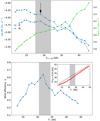 |
Fig. 1 Mass-loss rates Ṁ and Ṁt (top panel, dashed and solid blue lines, respectively), terminal velocities ν∞ (top panel, in green), and wind efficiency parameters η for the T* sequence of Z* = Z⊙ atmosphere models. The shaded region denotes the transition regions of two wind regimes. The arrow denotes the T* where η overturns. |
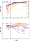 |
Fig. 2 Individual radiative accelerations throughout the wind of Fe IV (top panel) and Fe V (bottom panel), afe IV and afeV for the Z* = Z⊙ sequence. Both accelerations are normalized by g. The models at the turnover in Fig. 1 are highlighted; the T* = 32 kK model is shown as solid dotted lines, and T* = 33 kK is shown as dashed lines. |
3.3 Spectral imprint
The spectral appearance of WR stars is significantly affected by the wind stratification. Even in the case of ß-type velocity laws, the effect on the choice of β for the observed emission lines can be significant (see, e.g., Lefever et al. 2023). In Fig. 3 we show example spectra from our Z⊙ sequence for models with T* = 31, 32, 33 and 34 kK, that is, in the region in which η turns over (see also Fig. 1). Including some of the diagnostic lines from the WN-star classification by Smith et al. (1996), we plot the optical NIII λ4640 Å, HeII λ4686 Å, HeI λ5411 Å, and HeI λ5875 Å, as well as the CIV λλ 1550 Å UV line to illustrate the effect on the P Cygni lines. From the raw temperature effect on the spectra, one expects the spectral lines to show some gradual changes over this 3 kK range. Because of the inherent coupling with different wind parameters, the spectra actually display a sharper difference between T* = 32 and 33 kK. This is especially clear for the He I and He II lines in Fig. 3. he hotter models show weaker He I lines as expected. In contrast, the NIII λ 4640 Å lines show a different behavior. The 31 and 33 kK models are similar to each other, on the one hand, and the 32 and 34 kK models are similar to each other, on the other hand. As discussed in detail by Rivero González et al. (2011) the origin of these 3d→3p nitrogen-lines is complex. In O-stars, these lines can originate in the (quasi-)hydrostatic layers and still be in emission as a result of non-LTE effects. Depending on the model assumptions and the atomic data treatment, the line predictions can change considerably (see, e.g., the recent comparison in Sander et al. 2024). For WR stars, they eventually become wind lines, but are still very sensitive to the velocity, and thus, to the density. As reflected by our η and Ṁt values, the winds of our models are not that dense, despite the nominally high mass-loss rates. Hence, even when the changes in Ṁ and ν∞ between two models are moderate, the exact hydrodynamic solution in the wind onset region can overturn the gradual temperature effects on the spectral lines. This is different for the UV CIV λλ 1550 Å line, where the absorption is produced in the outer wind and the changes are only gradual. This confirms that the transitions of the global wind behavior are rather smooth for Z⊙.
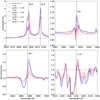 |
Fig. 3 Selection of optical diagnostic lines commonly used to determine the WN-star spectral type (see Smith et al. 1996) (top panels and bottom left panel), and the CIV λλ 1550 Å P Cygni profile. The four selected model spectra go over the turnover shown in Fig. 1. |
3.4 Effect of the metallicity
After examining the Z⊙-sequence, we studied additional model sequences at different metallicities from 1.2 to 0.02 Z⊙ (see Table 1 for an overview of the models per temperature and metal-licity). The Ṁ and ν∞ values of all temperature sequences except solar are shown in Fig. 4, similarly to the top panel in Fig. 1. Iron driving and spectral imprint plots similar to Figs. 2 and 3 can be found in Appendices B and C, respectively.
1.2Z. At supersolar metallicity, the behavior is generally similar to the solar metallicity case (see Fig. 4): There is an overturn in Ṁ, but now in double-peak form, and a flattening of Ṁt for cool temperatures. On the hot side, a strong decrease with temperature is again obtained. As in the Z⊙ case, two different wind regimes can be distinguished based on the difference in the aFe IV and aFe IV trends This is shown in the left panel of Fig. B.1. The exact point of the transition between the regimes is less clear because these models are close to the Eddington limit and because the radiative force in this (even moderately) supersolar regime is so high that models with T* between 32 and 36 kK did not converge within the same model setup. Based on the results of the Z⊙ models and because the wind efficiency of the 1.2 Z⊙ models peaked at 31 kK, we expect the transition to occur similarly smoothly, now at T* ≈ 31-32 kK.
0.8 Z. A different type of behavior occurs for the transition to subsolar metallicity. A clear trend discontinuity (jump) occurs between T* = and 33 kK in Ṁ and ν∞. The changes in aFeIV and aFeV (see the top-right panel in Fig. B.1) are now very distinct over this jump, in contrast to Z⊙. Moreover, at Z⊙, the trend in Ṁt started to flatten where η peaks, which also aligned with the iron switch. This is not the case in the 0.8 Z⊙ sequence, where η peaks at 29 kK, that is, below the iron switch. Similar to Z⊙, however, Ṁ peaks where η peaks and Ṁt approximately flattens for cooler temperatures.
The sharp drop between T* = 32 and 33 kK also results in a decrease in η by a factor of two. Interestingly, at T*≥ 34 kK, the wind regime seems to recover to the trend started on the cool side of the jump, and then to then to drop again for models where T* ≥ 40 kK.
0.6 Z⊙. When the metallicity is decreased further, the Ṁ- and ν∞ trends showed a sharp jump (see the middle left panel in Fig. 4), which now occured between T* = 33 and 34 kK. Below the jump, Ṁ was approximately constant before it eventually decreased again.
This behavior shows similarities to the bistability jump in the B supergiant models from Vink et al. (1999). The wind velocity stratification now clearly shows two separates regimes as depicted in Fig. 5. This did not occur for 1.2 Z⊙ and Z⊙ metallici-ties. For the 0.8 Z⊙ sequence, the situation is less clear. The jump in the 0.6 Z⊙ sequence coincides with differences in the aFe IV and aFe V stratifications (see the left panel of Fig. B.2). The position of the jump does not exactly coincide with Fe IV, however, taking over from FeV at Rcrit. On both sides, FeV is the leading line contribution at Rcrit, and although the importance of Fe IV increases continually, it only becomes the lead line acceleration at 30kK and below. At 29 kK, Ṁ, η, and Ṁt reach their peak values in the 0.6 Z⊙ sequence. The regime below shows a slight scatter in the Ṁ and Ṁt trend.
In Fig. 6 we show the corresponding spectra across the jump between 33 and 34 kK. The changes in Ṁ are now clearly visible in the lines (except for the aforementioned N III lines) while the change in ν is only evident in the UV.
0.4 Z⊙. The behavior of the 0.4 Z⊙ sequence is very similar to that of the 0.6 Z⊙ sequence. Again, there is a sharp jump in Ṁ and ν∞ between 33 and 34 kK and an approximately constant Ṁ for the temperatures below, as well as clear stratification differences in ν(r). The similarities are also visible in the aFe IV and aFeV stratification (see the left panel of Fig. D.2 and the right panels of Fig. B.2) and the spectral imprint (see Fig. C.5). The η turnover now occurs at 28 kK, but is otherwise in a similar fashion as for the 0.8 and 0.6 Z⊙ sequences.
0.2-0.02 Z⊙. At the lowest metallicity values studied in this work, the hotter models hardly converge to a solution within the given framework. For example, we find an upper limit of −6.48 for the 36kK model at 0.2Z⊙, but the model would not be considered converged by the same criteria as the other models. Showing only those models that converged within the same set of criteria in Fig. 4, we can only resolve the beginning of the jump at 0.2 Z⊙ (between 33 and 35 kK). The jump heavily influences the wind stratification (see Figs. D.2 and B.3) and the spectra (see Fig. C.5), similar to the 0.6 Z⊙ and 0.4 Z⊙ sequences. On the hotter side, the trend in η no longer turns over, but flattens for T* ≤ 29 kK. This is a consequence of Ṁ no longer decreasing for the coolest models.
For the 0.1 Z⊙−0.02 Z⊙ sequences, the general picture is similar to that of the 0.2 Z⊙ sequence with iron becoming even less important. Within the T* regime we covered, we no longer find a jump. While there is a some discontinuity in the M⊙ trend between 27 and 28 kK for 0.1 Z⊙, there is no dramatic drop of M⊙, but a rather continuous downward trend in the temperature range where we found the jump at higher Z. There is no local maximum in Ṁ, but the η values seem to settle for the cool-temperature end of our sequence. As we discuss further in Sect. 4, the main driving ingredients in this low-metallicity regime change. The wind-launching opacity bump formed by N III and N IV is further supported by other elemental ions, most notably S V and O IV. Carbon hardly plays a role because of the assumed WN-type composition we assumed, where most carbon has been transformed into nitrogen.
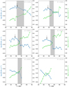 |
Fig. 4 Similar to Fig. 1, but now for other Z* sequences (denoted in gray in the top right corner of each panel). The Ṁ values are plotted in blue, and the ν∞ values are shown in green; The shaded regions and arrows denote the wind regime change and the turnover in η, respectively, if present. |
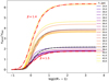 |
Fig. 5 Velocity fields for the 0.6 Z⊙ temperature sequence. Similar to Fig. 2, the models adjacent to the sharp wind transition are shown. The dotted solid lines show the T* = 33 kK model, and dashed lines show the 34 kK model. Two β velocity laws are shown, with β such that they fit the coolest and hottest models closest. |
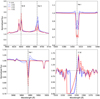 |
Fig. 6 Similar to Fig. 3, but here for the Z = 0.6 Z⊙ sequence and with models over the sharp wind transition. An overview of the same models in the K band is shown in Fig. C.1. |
4 Discussion
4.1 The turnover of Ṁ at low temperatures and higher metallicities
In all of the sequences between 1.2 Z⊙ and 0.4 Z⊙, we find that Ṁ and thus also η no longer increases monotonously with lower T*, but reach a maximum and eventually decline again. A more detailed inspection of the radiative accelerations of all models revealed that this is most likely related to a small opacity peak resulting from the FeV to FeVI recombination. At the hot side of the turnover, this opacity bump is located immediately below the wind launching at Rcrit, and it thus helps to boost the massloss rate. For cooler temperatures, this bump moves inward, now slightly below the wind-launching region. There, the peak is not sufficient to launch the wind in our current framework, but it affects the solution depending on whether or not a small superEddington regime has to be suppressed. Above this bump, a dip occurs in the Fe IV acceleration, which leads to a reduction in Ṁ. A similar effect was observed for OB star winds by Muijres et al. (2011) and Vink & Sander (2021). The magnitude of the dip is also connected to the scatter in Ṁ in the T* regime below the maximum. Eventually, Ṁ is expected to rise again when the repeated increase in the Fe IV acceleration reaches Rcrit, but this does not yet occur for our coolest models in the sequences.
Whether this overturn in the mass-loss rate is realized in nature is an open question. As demonstrated by Moens et al. (2022) and Debnath et al. (2024), radiatioy-driven turbulence might occur for a near- or super-Eddington opacity bump slightly below the stellar surface. As we demonstrate in González-Tora et al. (2025), this can affect the wind-launching solution and thus might cancel the effects of the bump. A study of this would require a depth-dependent implementation of turbulent pressure, however, which is beyond the scope of the current work.
For the lowest metallicities (Z ≤ 0.2 Z⊙), the turnover no longer occurs. This is a natural consequence of the diminished importance of iron, which no longer dominates the wind solution.
4.2 Strong discontinuities (jumps) in the Ṁ trend
For several but not all metallicities, we obtained a strong jump in the Ṁ(T*) trend. Interestingly, the jump is absent at Z ≥1.0Z⊙, but is present between 0.8 and 0.4Z⊙. This might initially seem counterintuitive because the role of line opacities at higher metallicities becomes more important. While the jump occurs close to the Fe V to Fe IV recombination regime, the inspection of our models indicated that this is not an immediate consequence of this ionization switch. It becomes especially evident in the 0.4 Z⊙ sequence, where the leading acceleration does not change at the same T* at which the jump in Ṁ occurs. The jump is instead the consequence ofa change in the iron opacity behavior. On the cool side of the jump, where Ṁ is significantly higher, the flux (F(r)) weighted mean iron opacity
 (4)
(4)
increases outward at Rcrit, while this is not the case for the hotter models with the lower mass-loss rate. As pointed out by Nugis & Lamers (2002), ξF must increase at Rcrit to for stable wind solution. If the leading Fe ion opacity does not provide this, other less efficient line opacities either from a different Fe stage or from an element such as nitrogen will eventually provide this when the mass-loss rate is reduced. When the two Fe ions do not contribute to an increasing opacity over Rcrit at a certain T*, but contribute for the next-cooler model, a large jump in Ṁ is obtained. This effect is shown in Fig. 7 in for the 0.8 Z⊙ sequence.
In the high-metallicity cases without a jump (e.g., at Z* = Z⊙), no split in the iron opacity gradient into an increasing and decreasing regime over Rcrit occurs. The κF-values continue to increase outward for all models, however. For the lowest metallicities, on the other hand (Z ≤ 0.2 Z⊙), the role of iron is no longer important enough to dominate the wind solution. Nitrogen instead becomes the leading line opacity and shows an outward-increasing χF around Rcrit for the whole model sequence, thereby preventing any strong discontinuities in Ṁ. Vink et al. (2001) described that carbon took over from iron as the main driver at low metallicity. We observed no minor jump behaviour caused by (e.g., carbon) recombination effects in the low-metallicity case, however.
It is currently unclear whether the obtained sharp discontinuities might be smeared out by multidimensional effects. In current multidimensional simulation efforts (e.g., Moens et al. 2022; Debnath et al. 2024), significant fluctuations in the temperature are seen throughout the wind. They reach differences of 10kK and more. If this were to very roughly correspond to an averaging between different 1D T* solutions, we cannot rule out that our obtained jumps in the Ṁ trend would be considerably reduced by multidimensional effects.
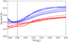 |
Fig. 7 Flux-weighted mean opacities χF for iron ions of the 0.8 Z⊙ sequence. The blue curves represent the blue side of the Ṁ jump in Fig. 4, where the red curves represent the hot side. |
4.3 WNh wind driving at very low metallicities
In all our models, the recombination of He III to He II only occurs beyond Rcrit. Despite the important role of iron, the Thomson free-electron contribution therefore outweighs the acceleration of any specific element at Rcrit at all metallicities. This is also illustrated in the three examples in Fig. 8, which show the most important contributions to the total wind acceleration atot in the wind onset region for three different models. Because Γe(r) is rather smooth, however, the wind solutions are dominated by the acceleration terms, which vary more strongly radially. At Z ≤ 0.2 Z⊙, the role of the Fe opacities becomes so weak in our models, that other opacity sources eventually take over. This is illustrated in the bottom panel of Fig. 8, where in particular nitrogen opacities of NIII and NIV and (at T* ≲ 29 kK) also the bound-free opacity from the continuum transitions of He II are the leading ion contributions at Rcrit. S IV and S V ions also play a role as do individual ions of elements such as C, Si, or Ar.
The complex Fe opacity no longer sets the overall Ṁ trend, and the mass-loss rate decreases with lower T*, driven by the combined continuum and line accelerations mentioned above. Interestingly, this trend is smoother than we find otherwise in our sample. As illustrated in Fig. 9, this regime closely resembles the relation
 (5)
(5)
that was found for the dense-wind regime of cWR stars by Sander et al. (2023). Although this is a very different parameter regime, this means that the pure geometrical effect from the lower temperature, that is, the implied lower log g(Rcrit), is the dominant reason for the increase in Ṁ. We ran a few models for even lower metallicities of 0.06 Z⊙ and 0.02 Z⊙ in this comparably higher mass-loss regime and found a similar trend, but shifted to lower Ṁ, as expected by the further decreasing line opacities.
In the outer wind, different ions contribute to the wind, depending on T*. For lower temperatures, FeIV still has an impact similar to carbon, nitrogen, and sulfur there at 0.1 Z⊙. For hotter models, iron hardly plays a role in the outer wind, but argon becomes more important instead, while nitrogen, carbon and sulfur maintain their prominent role.
For the coolest models and Z ≤ 0.1 Z⊙, the terminal velocities become very low (ν∞ ≲ 500 km s−1). Here, the radiative acceleration alone would not be sufficient to sustain the outer wind, but the slowly falling 1/r-term from the gas pressure contribution helps the material to escape. This is also evident from the resulting velocity fields shown in Fig. 10, where we obtain a nonmonotonic solution from the hydrodynamic equation of motion for the cool model3. A similar dichotomy is obtained in models with an even lower metallicity of 0.06 Z⊙ and 0.02 Z⊙ (in the same T* region). With decreasing Z, ν∞ first increases due to the effect of the decreasing Ṁ. he opacity in the wind that supports higher ν∞ eventually also decreases, however, and thus ν∞ again decreases.
In Fig. 11 we illustrate the Ṁ and the corresponding ν∞(Z) trend resulting from the models with T* = 26 kK, which is slightly hotter than the aforementioned coolest models, and thus, it does not correspond to the highest mass-loss regime at (very) low metallicity (see the bottom right panel in Fig. 13). The overall behavior is still the same, with ν∞ tending to increase due to weaker Ṁ, but it also needs to decrease because the available line opacity decreases. Despite the huge change in Ṁ, this example shows that ν∞ mainly scatters around the same order of values despite the significant changes in Z. This approximately constant ν(Z) trend is not obtained for the hotter models, which behave more similar to the classical WR stars in Sander & Vink (2020). For example, the 35 kK models change from ν = 1209 km s−1 at Z⊙ to 3408 km s−1 at 0.1 Z⊙. This change by more than 2000 km s−1 is accompanied by a decrease in Ṁ by about 1.6 dex, similar to what we see in Fig. 11 despite the very different ν behavior.
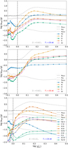 |
Fig. 8 Top two panels: main contributions to the total wind acceleration atot for a hot (top) and cold (midlle) model from the 0.6 Z⊙ sequence. The main elemental contributions to the summed radiative acceleration arad are indicated as well. The bottom panel shows the 0.1 Z⊙ model at T*, = 25 kK, but now lists the strongest contributions from individual ions to arad. |
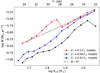 |
Fig. 9 Ṁ values shown at critical radii Rcrit for low-metallicity sequences of 0.1, 0.06, and 0.02 Z⊙. The dashed line represents the geometric effect of |

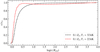 |
Fig. 10 Different types of velocity fields obtained in the low-metallicity regime. The hot model shows a typical radiation-driven wind settling on a terminal velocity, and the cool model shows a deceleration region and then a shallow, but continuously increasing velocity. |
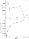 |
Fig. 11 Terminal wind velocities (top) and mass-loss rates (bottom) in terms of metallicity at T* = 26 kK. |
4.4 Comparison to Previous WNh Modeling
In Fig. 12 we show an example from the current WNh sequence compared to a model where Tmax = 100 and that launches its wind from the hot iron opacity bump, but has otherwise the same fundamental stellar parameters and also a similar effective temperature T2/3. While the terminal velocities differ by only ≈200 km s−1 (2030 km s−1 for the deep model versus 2260 km s−1 for the shallow model), the mass-loss rates differ by 1.46 dex (−3.80 versus −5.26). The combination of T2/3 and the line strengths in the spectrum can thus provide an immediate insight into the structure of the deeper atmosphere layers and the windlaunching regime. We therefore can conclude that most known WNh stars that reside on and below the main sequence cannot have winds that are launched by the hot iron bump.
The qualitatively different behavior of the wind regime we studied compared to the wind regime launched by the hot iron bump is also evident. In Fig. 13 we compare the T2/3 trend of the transformed mass-loss rate. For the comparison sequence at Z⊙, we obtain a smooth downward trend with increasing T2/3, while our model series shows a qualitatively different slope with much more substructure.
Based on an set of dynamically consistent models calculated with an earlier version of PoWR (e.g., containing a more limited set of elements and ions), Gräfener & Hamann (2008) derived a mass-loss recipe for WNh-type stars. While their recipe was anchored in the analysis of the hotter WN7h star WR 22 (T* = 44.7 kK), their models also covered a regime down to 31.6 kK. We extrapolated their derived formula and show the comparison of our models with their recipe in Fig. 14 for two different metal-licities. In the Z = Z⊙ case, the Ṁ values of our model sequence are of a similar order as their formula. The slightly higher values on average likely arise from the additional opacities that were included in the newer models. While the formula from Gräfener & Hamann (2008) reflected all the scatter in their individual models, our model trends show more substructure than in their model sets. While this might partially result from the additional complexity of the newer models, the prominent flattening of the Ṁ trend toward cooler temperatures does not occur in Gräfener & Hamann (2008) because this only occurs at the edge and beyond their grid coverage, that is, for T* ≤ 32 kK. This is even more relevant for the 0.4 Z⊙ sequence, where the Gräfener & Hamann (2008) formula essentially only covers the regime of lower mass-loss rates. On the cooler side of the Ṁ jump, the difference in mass-loss rate is almost an order of magnitude for some temperatures.
More recently, Bestenlehner (2020) suggested a mass-loss recipe for the Of to WNh regime based on empirical results in the Large Magellanic Cloud Tarantula region. As there is no explicit metallicity and temperature dependence, we highlight the covered M⊙ range in Fig. 14, using the calibration values from Brands et al. (2022). Notably, this region agrees with the cooler part of our 0.4 Z⊙ sequence, that is, the part with higher mass-loss rates, while there is a difference of about half an order of magnitude on the hotter side. We note, however, that the nature of the objects we modeled is likely different from most of the Large Magellanic Cloud R136 stars because their hydrogen surface abundances are higher, which would boost the resulting mass-loss rates (for the same L/Ṁ), as shown by Sander et al. (2023); Sander (2024).
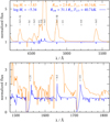 |
Fig. 12 Comparison of the optical (upper panel) and UV (lower panel) spectrum for a PoWRHD model from the current WNh sequence with a shallow wind launching (T* = 42 kK, blue) compared to model with a similar T2/3 (and ν∞) but with a deep wind launching (T* = 115 kK, orange). The two models share the same L, Ṁ, and chemical composition, but differ significantly in log Ṁt. |
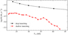 |
Fig. 13 Comparison of Ṁt vs. T2/3 between the Z⊙ PoWRHD model sequence with a shallow wind launching (red) and models with the same stellar parameters, but a deep wind launching (black). |
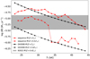 |
Fig. 14 Comparison of the Z⊙ model sequence with the Ṁ(Z) recipe from Gräfener & Hamann (2008, GH2008), where we display the Z = Z⊙ and 0.4 Z⊙ cases (in black). The shaded area represents the Ṁ range resulting from the recipe by Brands et al. (2022, B2022), for the different Γe of our Z = 0.4 sequence. |
4.5 Spectral appearance and WR definition
Wolf-Rayet stars are formally a spectroscopic definition, which raises the question whether our models with low mass-loss rates qualify for being classified as WR. The criteria for classification as a WR star vary between different temperature regimes. For the transition between early-O and mid-type WNh stars, which corresponds to objects that are located near or on the zero-age main sequence in the HRD, Hß is the main qualifier (Crowther & Walborn 2011). Hß in emission defines a WR star. Cooler objects with a mixture of absorption and emission lines are sometimes summarized under the label Ofpe/WN9, but as Crowther et al. (1995) and Crowther & Smith (1997) argued, the WN sequence can be extended to lower ionization stages. As HeII 4686Å can be in emission in O supergiants, they suggested using the occurrence of blueshifted absorption or narrow emission features in HeII4542Å (or 5412 Å) and HeI4471Å (or 5876 Å) to distinguish between wind-dominated and thus WN-defining spectra and mainly photospheric spectra.
In Fig. 15 we show a sequence of spectra at different metal-licities for the same T*. At solar-like metallicities, the spectra clearly are of WN type, but this changes with lower Z. At 0.2Z⊙, small emissions features remain, for example, in He II 4542 Å, while HeII 5412 Å appears to be in pure absorption already. At 0.06 Z⊙ and below, none of the lines except for HeII4686Å is in emission, although some traces of electron-scattering wings can still be noted for a few HeI and He II lines given the proximity to the Eddington limit. The spectra in Fig. 15 correspond to the model sequence plotted in Fig. 11, meaning that the terminal velocities do not change much throughout this particular sequence. These models, with their late-type WNh-star characteristic parameters, no longer have spectra that will be seen as WR-star spectra at lower metallicities. From Z ≲ 0.2 Z⊙ on, diagnostic lines in emission for WR stars are now in absorption, which additionally signals that the winds become comparatively very thin in the low Z regime. Hence, there is a transition from stars that show clear characteristics for late-type WNh stars at higher metallicities to stars with some wind imprint on the spectra but no longer a sufficiently strong wind to cause WR-like spectra.
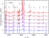 |
Fig. 15 Optical spectra of T* = 26 kK for different metallicities with the offset by increasing metallicity. |
5 Summary and conclusions
The in-depth analyses of late-type hydrogen-rich WR star models with our T* sequences revealed a range of remarkable properties in this regime near the Eddington limit. Ranging from supersolar to sub-SMC metallicities, myriad effects are seen that not all occur in other WR-star parameter ranges (e.g. at higher T* in Sander et al. 2023). At solar metallicity, an overturn in both the mass-loss rates and wind efficiencies is seen. After an initial increase in Ṁ for rising T*, the overall trend decreases for models where T* ≳ 25 kK. In addition, the behavior for the wind efficiency is similar, where the η values peak at 32 kK instead. This also occurs at supersolar metallicities, where the trends in global wind parameters are the same overall. For subsolar metallicity models with 0.4 Z⊙ ≤ Z ≤ 0.8 Z⊙, this same overturn for Ṁ and η is observed. This now coincides at around the same T* values while the temperatures at which these maxima occur drop systematically for decreasing Z. These maxima can be related to an increase in iron opacity χF as a result of the Fe V to Fe IV recombination, which tends to peak at the T* at which the turnover occurs. At SMC and sub-SMC metallcities Z ≲ 0.2Z⊙, these global wind maxima no longer seem to be present or fall below the temperature range of our models.
A striking feature we observed is the jump in Ṁ values for our 0.4 Z⊙ ≤ Z ≤ 0.8 Z⊙ model sequences. Here, our models are clearly separated in a hot and a cool side, where the wind characteristics differ significantly. On the cool side of these jumps, the winds typically show significantly higher Ṁ and lower ν∞, and vice versa on the hot side. The T* values at which this jump occurs range from 32 to 34 kK. This sharp difference in the wind regime also translates into wind stratification (e.g., the velocity fields in Appendix D and the line accelerations in Appendix C) and spectral differences, the latter especially in the case of strongly wind-affected lines in the UV (see Appendix B). In a number of ways, this sharp transition of the wind regimes is reminiscent of the classical bistability jump (see e.g. Vink et al. 1999, 2001). By studying the iron opacity χF stratification in our wind models, we can clearly distinguish two opacity groups in the sequences in which the jump occurs. While the classical bistability jump is described to be caused by the recombination of Fe IV to Fe III, the situation in our models is more complex, however. While generally, Fe V recombines to Fe IV and the lead iron ion driving in the temperature ranges of our model sequences switches, this does not necessarily lead to a sharp jump in the wind behavior, which is the case for Z ≥ Z⊙ models. Instead, we here distinguish two regimes on the basis of overall χF considerations: on the cool side of the jump, these models typically have a clear χF increase on and around the critical point Rcrit. On the hot side, this χF tends to plateau instead.
These two main effects, the Ṁ-η turnover and the Ṁ jumps, do not occur clearly or at all for our lower-metallicity sequences at Z ≤ 0.2Z⊙. At these Z, the contribution of iron to the wind driving starts to diminish and so do the effects of the iron opacities. Here, other opacity sources dominate the driving of the wind, that is, line opacities from e.g. N III, NIV and C IV along with continuum opacities from H I and He II. WITH the low impact of iron on the wind driving, the models agree better with the results from studies of cWR stars (e.g., Sander et al. 2023). At sub-SMC metallicities (Z ≤ 0.1 Z⊙), the radiation driving no longer suffices to continue to drive the wind material farther out in the wind. Acceleration from the pressure gradient instead takes over as the main driver there.
These model sequences show significant differences to previous studies, in which the winds were typically launched at high optical depths τ. The main cause of this is that the models we used are launched at shallow depths τ, in contrast to previous work, where the winds were typically thought to be launched at the hot iron bump. Spectroscopically, our models tend to represent nature better with more physically realistic spectra, where there is a general drop of an order of magnitude in the mass-loss rates we find for this type of star. We note that our atmosphere models and the resulting spectra are representative for luminous late-type WNh stars, thought to be burning their core H. Our results should not be directly extrapolated to all WNh-type stars because they might have very different combinations of stellar parameters, which would cause a different wind behavior from what we observed in our model sequences. Additional model sequences covering further parameter regimes are required to combine our work with other recent work into an improved mass-loss description for (cooler) WNh-type stars.
This range of effects and the insights into the wind behavior, along with the numerous spectral considerations from our analyses, shows that future work requires observational studies on late-type WNh stars that take our results into account. This is exactly the theme of a planned follow-up study, that will compare previous results for WNh stars in the Galactic center with novel spectroscopic analysis using a hydrodynamically consistent modeling.
Data availability
Appendices B (radiative accelerations), C (spectra) and D (velocity fields) and figures therein are found in https://doi.org/10.5281/zenodo.15675082
Acknowledgements
A.A.C.S., M.B.P., and R.R.L. are supported by the Deutsche Forschungsgemeinschaft (DFG, German Research Foundation) in the form of an Emmy Noether Research Group - Project-ID 445674056 (SA4064/1-1, PI: Sander). A.A.C.S. and R.R.L. further acknowledge support from the Deutsche Forschungsgemeinschaft (DFG, German Research Foundation) - Project-ID 138713538 -SFB 881 (“The Milky Way System”, subproject P04). This project was co-funded by the European Union (Project 101183150 - OCEANS). G.N.S. and J.S.V. are supported by STFC (Science and Technology Facilities Council) funding under grant number ST/Y001338/1. R.R.L. is a member of the International Max Planck Research School for Astronomy and Cosmic Physics at the University of Heidelberg (IMP.RS-HD). N.M. acknowledges the support of the European Research Council (ERC) Horizon Europe grant under grant agreement number 101044048. F.N. acknowledges support by PID2022-137779OB-C41 funded by MCIN/AEI/10.13039/501100011033 by “ERDF A way of making Europe”.
Appendix A Model abundances
In Table A.1, we provide an overview of the abundances and ions entering the atmosphere model calculations prestented in this work. The specific mass fractions listed in table A.1 only refer to the sequence marked as solar metallicity Z⊙. For the sequences with different metallicities, we keep the same XH, but scale metals (N to Fe) with Z/Z⊙. The He mass fraction then follows as  .
.
Elements, ions and their respective abundances in mass fractions Xm used in this work for the Z = Z⊙-sequencea,b.
References
- Abbott, R., Abbott, T. D., Abraham, S., et al. 2021, Phys. Rev. D, 103, 122002 [NASA ADS] [CrossRef] [Google Scholar]
- Asplund, M., Grevesse, N., Sauval, A. J., & Scott, P. 2009, ARA&A, 47, 481 [NASA ADS] [CrossRef] [Google Scholar]
- Barniske, A., Oskinova, L. M., & Hamann, W. R. 2008, A&A, 486, 971 [NASA ADS] [CrossRef] [EDP Sciences] [Google Scholar]
- Bestenlehner, J. M. 2020, MNRAS, 493, 3938 [Google Scholar]
- Brands, S. A., de Koter, A., Bestenlehner, J. M., et al. 2022, A&A, 663, A36 [Google Scholar]
- Clark, J. S., Lohr, M. E., Patrick, L. R., et al. 2018, A&A, 618, A2 [NASA ADS] [CrossRef] [EDP Sciences] [Google Scholar]
- Conti, P. S., Garmany, C. D., De Loore, C., & Vanbeveren, D. 1983, ApJ, 274, 302 [NASA ADS] [CrossRef] [Google Scholar]
- Crowther, P. A. 2007, ARA&A, 45, 177 [Google Scholar]
- Crowther, P. A., & Hadfield, L. J. 2006, A&A, 449, 711 [NASA ADS] [CrossRef] [EDP Sciences] [Google Scholar]
- Crowther, P. A., & Smith, L. J. 1997, A&A, 320, 500 [NASA ADS] [Google Scholar]
- Crowther, P. A., & Walborn, N. R. 2011, MNRAS, 416, 1311 [Google Scholar]
- Crowther, P. A., Hillier, D. J., & Smith, L. J. 1995, A&A, 293, 172 [NASA ADS] [Google Scholar]
- Crowther, P. A., Dessart, L., Hillier, D. J., Abbott, J. B., & Fullerton, A. W. 2002, A&A, 392, 653 [NASA ADS] [CrossRef] [EDP Sciences] [Google Scholar]
- de Koter, A., Heap, S. R., & Hubeny, I. 1997, ApJ, 477, 792 [Google Scholar]
- Debnath, D., Sundqvist, J. O., Moens, N., et al. 2024, A&A, 684, A177 [NASA ADS] [CrossRef] [EDP Sciences] [Google Scholar]
- Dray, L. M., & Tout, C. A. 2003, MNRAS, 341, 299 [Google Scholar]
- Farmer, R., Laplace, E., de Mink, S. E., & Justham, S. 2021, ApJ, 923, 214 [NASA ADS] [CrossRef] [Google Scholar]
- González-Torà, G., Sander, A. A. C., Sundqvist, J. O., et al. 2025, A&A, 694, A269 [NASA ADS] [CrossRef] [EDP Sciences] [Google Scholar]
- Gräfener, G., & Hamann, W. R. 2005, A&A, 432, 633 [NASA ADS] [CrossRef] [EDP Sciences] [Google Scholar]
- Gräfener, G., & Hamann, W. R. 2008, A&A, 482, 945 [Google Scholar]
- Gräfener, G., & Vink, J. S. 2013, A&A, 560, A6 [NASA ADS] [CrossRef] [EDP Sciences] [Google Scholar]
- Gräfener, G., Koesterke, L., & Hamann, W. R. 2002, A&A, 387, 244 [NASA ADS] [CrossRef] [EDP Sciences] [Google Scholar]
- Hainich, R., Pasemann, D., Todt, H., et al. 2015, A&A, 581, A21 [NASA ADS] [CrossRef] [EDP Sciences] [Google Scholar]
- Hamann, W. R. 1985, A&A, 148, 364 [Google Scholar]
- Hamann, W. R., & Gräfener, G. 2003, A&A, 410, 993 [CrossRef] [EDP Sciences] [Google Scholar]
- Hamann, W. R., & Koesterke, L. 1998, A&A, 335, 1003 [Google Scholar]
- Hamann, W. R., Gräfener, G., & Liermann, A. 2006, A&A, 457, 1015 [NASA ADS] [CrossRef] [EDP Sciences] [Google Scholar]
- Higgins, E. R., Sander, A. A. C., Vink, J. S., & Hirschi, R. 2021, MNRAS, 505, 4874 [NASA ADS] [CrossRef] [Google Scholar]
- Hillier, D. J., & Miller, D. L. 1999, ApJ, 519, 354 [Google Scholar]
- Hillier, D. J., Lanz, T., Heap, S. R., et al. 2003, ApJ, 588, 1039 [Google Scholar]
- Hiltner, W. A., & Schild, R. E. 1966, ApJ, 143, 770 [NASA ADS] [CrossRef] [Google Scholar]
- Josiek, J., Sander, A. A. C., Bernini-Peron, M., et al. 2025, A&A, 697, A193 [NASA ADS] [CrossRef] [EDP Sciences] [Google Scholar]
- Lefever, R. R., Sander, A. A. C., Shenar, T., et al. 2023, MNRAS, 521, 1374 [NASA ADS] [CrossRef] [Google Scholar]
- Lenoir-Craig, G., Antokhin, I. I., Antokhina, E. A., St-Louis, N., & Moffat, A. F. J. 2022, MNRAS, 510, 246 [Google Scholar]
- Liermann, A., Hamann, W. R., & Oskinova, L. M. 2009, A&A, 494, 1137 [NASA ADS] [CrossRef] [EDP Sciences] [Google Scholar]
- Liermann, A., Hamann, W. R., Oskinova, L. M., Todt, H., & Butler, K. 2010, A&A, 524, A82 [NASA ADS] [CrossRef] [EDP Sciences] [Google Scholar]
- Maeder, A. 1983, A&A, 120, 113 [NASA ADS] [Google Scholar]
- Moens, N., Poniatowski, L. G., Hennicker, L., et al. 2022, A&A, 665, A42 [NASA ADS] [CrossRef] [EDP Sciences] [Google Scholar]
- Muijres, L. E., de Koter, A., Vink, J. S., et al. 2011, A&A, 526, A32 [NASA ADS] [CrossRef] [EDP Sciences] [Google Scholar]
- Nugis, T., & Lamers, H. 2002, A&A, 389, 162 [NASA ADS] [CrossRef] [EDP Sciences] [Google Scholar]
- Oskinova, L. M., Steinke, M., Hamann, W. R., et al. 2013, MNRAS, 436, 3357 [Google Scholar]
- Poniatowski, L. G., Sundqvist, J. O., Kee, N. D., et al. 2021, A&A, 647, A151 [NASA ADS] [CrossRef] [EDP Sciences] [Google Scholar]
- Rivero González, J. G., Puls, J., & Najarro, F. 2011, A&A, 536, A58 [NASA ADS] [CrossRef] [EDP Sciences] [Google Scholar]
- Sabhahit, G. N., Vink, J. S., Sander, A. A. C., & Higgins, E. R. 2023, MNRAS, 524, 1529 [NASA ADS] [CrossRef] [Google Scholar]
- Sabhahit, G. N., Vink, J. S., Sander, A. A. C., et al. 2025, A&A, 696, A200 [NASA ADS] [CrossRef] [EDP Sciences] [Google Scholar]
- Sander, A. A. C. 2024, IAU Symp., 361, 473 [Google Scholar]
- Sander, A. A. C., & Vink, J. S. 2020, MNRAS, 499, 873 [Google Scholar]
- Sander, A., Todt, H., Hainich, R., & Hamann, W. R. 2014, A&A, 563, A89 [NASA ADS] [CrossRef] [EDP Sciences] [Google Scholar]
- Sander, A., Shenar, T., Hainich, R., et al. 2015, A&A, 577, A13 [NASA ADS] [CrossRef] [EDP Sciences] [Google Scholar]
- Sander, A. A. C., Hamann, W. R., Todt, H., Hainich, R., & Shenar, T. 2017, A&A, 603, A86 [NASA ADS] [CrossRef] [EDP Sciences] [Google Scholar]
- Sander, A. A. C., Vink, J. S., & Hamann, W. R. 2020, MNRAS, 491, 4406 [Google Scholar]
- Sander, A. A. C., Lefever, R. R., Poniatowski, L. G., et al. 2023, A&A, 670, A83 [NASA ADS] [CrossRef] [EDP Sciences] [Google Scholar]
- Sander, A. A. C., Bouret, J. C., Bernini-Peron, M., et al. 2024, A&A, 689, A30 [NASA ADS] [CrossRef] [EDP Sciences] [Google Scholar]
- Scott, P., Asplund, M., Grevesse, N., Bergemann, M., & Sauval, A. J. 2015a, A&A, 573, A26 [NASA ADS] [CrossRef] [EDP Sciences] [Google Scholar]
- Scott, P., Grevesse, N., Asplund, M., et al. 2015b, A&A, 573, A25 [NASA ADS] [CrossRef] [EDP Sciences] [Google Scholar]
- Shenar, T., Hainich, R., Todt, H., et al. 2016, A&A, 591, A22 [NASA ADS] [CrossRef] [EDP Sciences] [Google Scholar]
- Shenar, T., Sablowski, D. P., Hainich, R., et al. 2019, A&A, 627, A151 [NASA ADS] [CrossRef] [EDP Sciences] [Google Scholar]
- Shenar, T., Sablowski, D. P., Hainich, R., et al. 2020, A&A, 641, C2 [NASA ADS] [CrossRef] [EDP Sciences] [Google Scholar]
- Smith, L. F. 1968, MNRAS, 138, 109 [NASA ADS] [CrossRef] [Google Scholar]
- Smith, N. 2014, ARA&A, 52, 487 [NASA ADS] [CrossRef] [Google Scholar]
- Smith, L. F., Shara, M. M., & Moffat, A. F. J. 1996, MNRAS, 281, 163 [NASA ADS] [CrossRef] [Google Scholar]
- Smith, L. J., Norris, R. P. F., & Crowther, P. A. 2002, MNRAS, 337, 1309 [CrossRef] [Google Scholar]
- Sundqvist, J. O., Björklund, R., Puls, J., & Najarro, F. 2019, A&A, 632, A126 [NASA ADS] [CrossRef] [EDP Sciences] [Google Scholar]
- Todt, H., Sander, A., Hainich, R., et al. 2015, A&A, 579, A75 [NASA ADS] [CrossRef] [EDP Sciences] [Google Scholar]
- Tramper, F., Straal, S. M., Sanyal, D., et al. 2015, A&A, 581, A110 [NASA ADS] [CrossRef] [EDP Sciences] [Google Scholar]
- Vink, J. S., & Sander, A. A. C. 2021, MNRAS, 504, 2051 [NASA ADS] [CrossRef] [Google Scholar]
- Vink, J. S., de Koter, A., & Lamers, H. J. G. L. M. 1999, A&A, 350, 181 [Google Scholar]
- Vink, J. S., de Koter, A., & Lamers, H. J. G. L. M. 2001, A&A, 369, 574 [NASA ADS] [CrossRef] [EDP Sciences] [Google Scholar]
- Vink, J. S., Higgins, E. R., Sander, A. A. C., & Sabhahit, G. N. 2021, MNRAS, 504, 146 [NASA ADS] [CrossRef] [Google Scholar]
- Woosley, S. E., Sukhbold, T., & Janka, H. T. 2020, ApJ, 896, 56 [NASA ADS] [CrossRef] [Google Scholar]
Our choice of τcont,max = 5 compared to the more common values of 20 and 100 also reduces the difference a bit.
Γe is defined similarly to the aforementioned Γrad, but only takes the acceleration due to (Thomson) electron scattering opacity into account.
For the radiative transfer calculation, the nonmonotonic part in ν(r) is interpolated as explained and illustrated by Sander et al. (2023).
All Tables
Elements, ions and their respective abundances in mass fractions Xm used in this work for the Z = Z⊙-sequencea,b.
All Figures
|
Fig. 1 Mass-loss rates Ṁ and Ṁt (top panel, dashed and solid blue lines, respectively), terminal velocities ν∞ (top panel, in green), and wind efficiency parameters η for the T* sequence of Z* = Z⊙ atmosphere models. The shaded region denotes the transition regions of two wind regimes. The arrow denotes the T* where η overturns. |
| In the text | |
|
Fig. 2 Individual radiative accelerations throughout the wind of Fe IV (top panel) and Fe V (bottom panel), afe IV and afeV for the Z* = Z⊙ sequence. Both accelerations are normalized by g. The models at the turnover in Fig. 1 are highlighted; the T* = 32 kK model is shown as solid dotted lines, and T* = 33 kK is shown as dashed lines. |
| In the text | |
|
Fig. 3 Selection of optical diagnostic lines commonly used to determine the WN-star spectral type (see Smith et al. 1996) (top panels and bottom left panel), and the CIV λλ 1550 Å P Cygni profile. The four selected model spectra go over the turnover shown in Fig. 1. |
| In the text | |
|
Fig. 4 Similar to Fig. 1, but now for other Z* sequences (denoted in gray in the top right corner of each panel). The Ṁ values are plotted in blue, and the ν∞ values are shown in green; The shaded regions and arrows denote the wind regime change and the turnover in η, respectively, if present. |
| In the text | |
|
Fig. 5 Velocity fields for the 0.6 Z⊙ temperature sequence. Similar to Fig. 2, the models adjacent to the sharp wind transition are shown. The dotted solid lines show the T* = 33 kK model, and dashed lines show the 34 kK model. Two β velocity laws are shown, with β such that they fit the coolest and hottest models closest. |
| In the text | |
|
Fig. 6 Similar to Fig. 3, but here for the Z = 0.6 Z⊙ sequence and with models over the sharp wind transition. An overview of the same models in the K band is shown in Fig. C.1. |
| In the text | |
|
Fig. 7 Flux-weighted mean opacities χF for iron ions of the 0.8 Z⊙ sequence. The blue curves represent the blue side of the Ṁ jump in Fig. 4, where the red curves represent the hot side. |
| In the text | |
|
Fig. 8 Top two panels: main contributions to the total wind acceleration atot for a hot (top) and cold (midlle) model from the 0.6 Z⊙ sequence. The main elemental contributions to the summed radiative acceleration arad are indicated as well. The bottom panel shows the 0.1 Z⊙ model at T*, = 25 kK, but now lists the strongest contributions from individual ions to arad. |
| In the text | |
|
Fig. 9 Ṁ values shown at critical radii Rcrit for low-metallicity sequences of 0.1, 0.06, and 0.02 Z⊙. The dashed line represents the geometric effect of |
| In the text | |
|
Fig. 10 Different types of velocity fields obtained in the low-metallicity regime. The hot model shows a typical radiation-driven wind settling on a terminal velocity, and the cool model shows a deceleration region and then a shallow, but continuously increasing velocity. |
| In the text | |
|
Fig. 11 Terminal wind velocities (top) and mass-loss rates (bottom) in terms of metallicity at T* = 26 kK. |
| In the text | |
|
Fig. 12 Comparison of the optical (upper panel) and UV (lower panel) spectrum for a PoWRHD model from the current WNh sequence with a shallow wind launching (T* = 42 kK, blue) compared to model with a similar T2/3 (and ν∞) but with a deep wind launching (T* = 115 kK, orange). The two models share the same L, Ṁ, and chemical composition, but differ significantly in log Ṁt. |
| In the text | |
|
Fig. 13 Comparison of Ṁt vs. T2/3 between the Z⊙ PoWRHD model sequence with a shallow wind launching (red) and models with the same stellar parameters, but a deep wind launching (black). |
| In the text | |
|
Fig. 14 Comparison of the Z⊙ model sequence with the Ṁ(Z) recipe from Gräfener & Hamann (2008, GH2008), where we display the Z = Z⊙ and 0.4 Z⊙ cases (in black). The shaded area represents the Ṁ range resulting from the recipe by Brands et al. (2022, B2022), for the different Γe of our Z = 0.4 sequence. |
| In the text | |
|
Fig. 15 Optical spectra of T* = 26 kK for different metallicities with the offset by increasing metallicity. |
| In the text | |
Current usage metrics show cumulative count of Article Views (full-text article views including HTML views, PDF and ePub downloads, according to the available data) and Abstracts Views on Vision4Press platform.
Data correspond to usage on the plateform after 2015. The current usage metrics is available 48-96 hours after online publication and is updated daily on week days.
Initial download of the metrics may take a while.