| Issue |
A&A
Volume 699, July 2025
|
|
|---|---|---|
| Article Number | A319 | |
| Number of page(s) | 9 | |
| Section | Interstellar and circumstellar matter | |
| DOI | https://doi.org/10.1051/0004-6361/202555333 | |
| Published online | 16 July 2025 | |
The Crab Nebula at sub-arcsecond resolution with the International LOFAR Telescope
1
ASTRON Netherlands Institute for Radio Astronomy,
Oude Hoogeveensedijk 4,
7991
PD
Dwingeloo,
The Netherlands
2
Anton Pannekoek Institute, University of Amsterdam,
Science Park 904,
1098
XH
Amsterdam,
The Netherlands
3
Centre for Extragalactic Astronomy, Department of Physics, Durham University,
Durham,
DH1 3LE,
UK
4
Institute for Computational Cosmology, Department of Physics, Durham University,
South Road,
Durham
DH1 3LE,
UK
5
Leiden Observatory, Leiden University,
PO Box 9513,
2300
RA
Leiden,
The Netherlands
★ Corresponding author: This email address is being protected from spambots. You need JavaScript enabled to view it.
Received:
29
April
2025
Accepted:
19
June
2025
Abstract
We present International LOw Frequency ARray (LOFAR) Telescope (ILT) observations of the Crab Nebula, the remnant of a core-collapse supernova explosion observed by astronomers in 1054. The field of the Crab Nebula was observed between 120 and 168 MHz as part of the LOFAR Two-Metre Sky Survey (LoTSS), and the data were re-processed to include the LOFAR international stations to create a high-angular-resolution (0.43″ × 0.28″) map at a central frequency of 145 MHz. Combining the ILT map with archival centimetre-range observations of the nebula with the Very Large Array (VLA) and LOFAR data at 54 MHz, we become sensitive to the effects of free-free absorption against the synchrotron emission of the pulsar wind nebula. This absorption is caused by the ionised filaments visible in optical and infrared data of the Crab Nebula, which are the result of the pulsar wind nebula expanding into the denser stellar ejecta that surrounds it and forming Rayleigh-Taylor fingers. The LOFAR observations are sensitive to two components of these filaments: their dense cores, which have electron densities of ≳1000 cm−3, and the diffuse envelopes, with electron densities of ~50–250 cm−3. The denser structures have widths of ~0.03 pc, whereas the diffuse component is at one point as large as 0.2 pc. The morphology of the two components is not always the same. These findings suggest that the layered temperature, density, and ionisation structure of the Crab optical filaments extends to larger scales than previously considered.
Key words: radiation mechanisms: non-thermal / ISM: supernova remnants / radio continuum: ISM / ISM: individual objects: Crab Nebula
© The Authors 2025
 Open Access article, published by EDP Sciences, under the terms of the Creative Commons Attribution License (https://creativecommons.org/licenses/by/4.0), which permits unrestricted use, distribution, and reproduction in any medium, provided the original work is properly cited.
This article is published in open access under the Subscribe to Open model. This email address is being protected from spambots. You need JavaScript enabled to view it. to support open access publication.
1 Introduction
The Crab Nebula is one of the most thoroughly observed objects in the Galaxy (Hester 2008). Its many names are a testament to its observational draw: it is called SN 1054 from the year it was observed as an optical transient by historical astronomers, Messier 1 for its optical nebula, 3C 144 and Taurus A for its radio nebula, and has the supernova remnant catalogue name of G 184.6–5.8. It is also one of the brightest sources in the radio sky, with a flux density at 1 GHz of 1042 ± 75 Jy (Baars et al. 1977).
The Crab Nebula consists of the Crab Pulsar (PSR B0531+21, the neutron star left behind in the supernova explosion), its synchrotron-emitting pulsar wind nebula, and a bright shell of thermally emitting stellar ejecta and swept-up interstellar material (Hester 2008). It might also have a faint, undetected supernova remnant shell that surrounds the other components (Sollerman et al. 2000). The pulsar wind nebula is confined by, and pushing into, the thermally emitting material; this results in Rayleigh-Taylor instabilities that give the appearance of a ‘cage’ of thermal filaments enclosing the synchrotron nebula (Chevalier & Gull 1975; Hester et al. 1996). The filaments are photoionised due to the radiation emitted by the synchrotron nebula and show a variety of ionisation states (e.g. Graham et al. 1990; Blair et al. 1992) in elements typically present in supernova ejecta, such as oxygen, sulfur, iron, and nickel (Temim et al. 2024). Throughout this work, we refer to the ‘pulsar wind nebula’ as the wind of relativistic particles powered by the loss of the rotational energy of the pulsar, and to the ‘supernova remnant’ as the expelled stellar ejecta and swept-up circumstellar and interstellar media, including the supernova blast wave that would be seen as an (as of now undetected) shell surrounding the complete structure that we call the Crab Nebula.
The ionisation structure of the ejecta filaments that enclose the pulsar wind nebula is layered, with lower ionisation states found in compact, sheltered cores surrounded by higherionisation envelopes. The filament cores also contain dust, which can be seen as extinction features against the synchrotron nebula (Sankrit et al. 1998; Owen & Barlow 2015). This geometry – an extended synchrotron source with ionised material in the foreground – can result in free-free absorption of the synchrotron emission at low radio frequencies (<100 MHz; Arias et al. 2018, 2019), provided that the foreground material is sufficiently dense and/or cold.
The Crab Nebula has been observed extensively in the radio, in particular with the Karl G. Jansky Very Large Array (VLA) in all its configurations and at a variety of observing frequencies (Bietenholz & Kronberg 1990; Kassim et al. 1993; Bietenholz et al. 2004, 2015). Its integrated radio spectral index is constant at α = −0.27 ± 0.04 (for Sν ∝ να) from 10 MHz to ~104 GHz (corresponding to the frequency of the synchrotron break; Bietenholz et al. 1997).
The ‘historical’ VLA, the array as it was before the upgrade completed in 2011, had two receivers at frequencies below 1 GHz: one at 74 MHz and one at 327 MHz. Combining observations at these frequencies with data at 1.5 GHz and 4.9 GHz, Bietenholz et al. (1997) carried out a radio spectral index study of the source with the aim of looking for spatial variations. The authors found that the spectral index of the nebula is spatially uniform between the 327 MHz, 1.4 GHz, and 4.9 GHz maps but that at 74 MHz there is an unresolved absorption feature, which they ascribe to free-free absorption from the brightest optical knot with a negative radial velocity. Here we confirm and expand on this interpretation with high-resolution, low-frequency imaging of the Crab Nebula.
The LOw Frequency ARray (LOFAR; van Haarlem et al. 2013) is a radio interferometer with a dense core located in and around Exloo, The Netherlands, and individual stations elsewhere in The Netherlands and Europe. When the Dutch LOFAR stations are combined with the remaining LOFAR international stations, the array is known as the International LOFAR Telescope (ILT) and provides sub-arcsecond resolution with its high-band antennas (HBAs) centred at 150 MHz. In this work we present low-frequency radio observations of the Crab Nebula with the ILT in which absorption effects due to the thermal filament cage surrounding the nebula are present and resolved.
In Sect. 2, we present the ILT observations and describe the ancillary data used in this work. In Sect. 3, we present spectral index maps of the Crab Nebula and the results of fitting the images at different frequencies as a synchrotron source subject to free-free absorption. We also quote a surface brightness upper limit at LOFAR frequencies for the, as of yet undetected, Crab Nebula supernova remnant shell. In Sect. 4, we discuss the implications of the LOFAR observations for the conditions in the absorbing Rayleigh-Taylor filaments, and in Sect. 5 we summarise our work.
2 Observations and data reduction
2.1 ILT observations
The observations used in this work were taken as part of the LOFAR Two-Metre Sky Survey (LoTSS; Shimwell et al. 2017, 2019, 2022), a survey with the LOFAR HBA at a central frequency of 145 MHz that covers 85% of the northern sky. Although the LoTSS data products are imaged using only the Dutch LOFAR stations, resulting in 6″ resolution and typically reaching sensitivities of ~100 μJy bm−1, most of the survey data were recorded using the full ILT array. This provides the option of re-processing the data to include the international stations, increasing the maximum baseline length and reaching an angular resolution of 0.3″.
The LoTSS observation covering the Crab Nebula was taken on 4 March 2023 for a total on-source integration time of 4 hours. The data were recorded in full linear polarisation mode between 120 and 168 MHz with a frequency channel width of 12 kHz and an integration interval of 1 second. In addition, the primary calibrator source 3C 48 was observed with the same observing setup for 10 minutes immediately afterwards.
The data on 3C48 were first processed using the PREFACTOR package (now the LOFAR Initial Calibration pipeline, LINC; van Weeren et al. 2016; Williams et al. 2016; de Gasperin et al. 2019) to obtain calibration solutions for the bandpass, the polarisation alignment, and the clock offsets for each LOFAR station. Next, these solutions were applied to the target data and an initial phase calibration cycle was performed by comparing the data for the Dutch stations against a sky model obtained from the TIFR GMRT Sky Survey (TGSS; Intema et al. 2017).
Following this initial calibration, the full international LOFAR array was calibrated using a bespoke strategy implemented using LOFAR very long baseline interferometry pipeline tools (Morabito et al. 2022; van Weeren et al. 2021). First, the data were phase-shifted to the coordinates of the Crab pulsar, converted to circular polarisation, and averaged to a channel width of 49 kHz and an integration interval of 4 seconds. Next, calibration solutions were derived for the full array on the central pulsar using only baselines exceeding 80 kλ to suppress the surrounding large-scale emission. This baseline cut causes the calibration to only consider emission on scales smaller than ~2.6 arcseconds. These calibration solutions include short-timescale phase corrections for left- and right-handed circular polarisations separately, as well as gain corrections to solve for the slowly varying gain of the array and to correct for giant pulses (Heiles & Campbell 1970) from the central pulsar. The giant pulses are intense bursts of radio emission occurring on nanosecond timescales, but emitting several orders of magnitude above the typical pulse flux (Karuppusamy et al. 2010). After deriving all calibration solutions and applying these to the data, the full Crab Nebula was imaged using WSCLEAN (Offringa et al. 2014). The resulting image is shown in Fig. 1.
2.2 Ancillary data
In addition to the LOFAR HBA data described above, we used archival and published radio data in order to conduct a spectral analysis of the source. We used the LOFAR low-band antenna (LBA) observations published in de Gasperin et al. (2020), centred at 54 MHz. We also used C-band data centred at 5450 MHz taken with the VLA and published in Bietenholz et al. (2015). Finally, we downloaded calibrated L-band visibilities from the VLA archive (Kent et al. 2018) and made an image centred at 1520 MHz. The properties of each image are summarised in Table 1.
3 Results
3.1 Spectral index maps
To correct for the expansion of the pulsar wind nebula in the time period between the LOFAR and the VLA observations, we spatially rescaled the LOFAR map with respect to the central pulsar. By eye, we estimate a scaling factor of 0.990 ± 0.001 in order to match features in the VLA maps to the LOFAR map better than the angular resolution. This correction agrees well with the difference in age of the Crab Nebula between the VLA and LOFAR epochs (Bietenholz et al. 2015). With this re-scaling applied, we created spectral index maps between the 145 and 1520 MHz maps (the LOFAR HBA and the VLA L band), and between the 54 and 1520 MHz maps (LOFAR LBA and the VLA L band). The results are shown in Fig. 2. For each spectral index map, the higher-resolution map was convolved with a Gaussian to match the resolution of the lower-resolution map as given in Table 1, and then re-gridded to match its grid.
The most prominent feature in the LBA to L band (54 MHz to 1.5 GHz) spectral index map is a filament south-west of the pulsar, which stands out as having a flatter spectral index (α ≈ 0) than the rest of the source (labelled ‘Filament 1’ in Fig. 2, left). As mentioned earlier, the presence of an (unresolved) flatter structure at this location was first noted by Bietenholz et al. (1997) from the analysis of VLA 74 MHz data. The authors attributed the spectral index flattening to free-free absorption by the thermal material in the optical filaments. This interpretation is further confirmed by the morphology of the 54 MHz to 1.5 GHz spectral index map: the regions of flat spectral index in yellow and green clearly trace the outline of the blueshifted (i.e. foreground) Rayleigh-Taylor fingers as seen in the optical and infrared (see e.g. Hester et al. 1996; Loll et al. 2013; Martin et al. 2021; Temim et al. 2024).
Filament 1 is also seen as the main feature in the HBA to L band (145 MHz to 1.5 GHz) spectral index map: a thin band of emission that partially encircles the pulsar from the south. Figure 3 shows a cutout of this feature in the spectral index map, alongside the HBA image and a Chandra X-ray map of the source (Weisskopf et al. 2012). The absorption effects here are so significant that the filament appears as a dark track in the LOFAR HBA total intensity map (Fig. 3, middle) and in the X-rays (Fig. 3, left). Figure 3 shows that Filament 1 is in fact inhomogeneous, and has knots of positive spectral index on its western side.
The HBA to L band (145 MHz to 1.5 GHz) spectral index map shows a gradient in spectral index seen from the south-east to the north-west. We cannot exclude the possibility that this feature is caused by residual primary beam effects: the source lies one degree from the phase centre of the LoTSS pointing that was re-processed to include the international stations and make the map in Fig. 1, and hence it is subject to edge effects when applying the primary beam correction. The extended feature of flatter spectral index that follows the semi-major axis of the nebula (coinciding with what is seen as a jet in the X-rays) does not show in the LBA to L band map (54 MHz to 1.5 GHz) and is also likely due to artefacts in the 145 MHz high-resolution map.
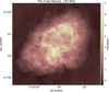 |
Fig. 1 The Crab Nebula as seen with the HBA of the ILT. This map has a central frequency of 145 MHz, an angular resolution of 0.43″ × 0.28″, an rms noise of 260 μJy bm−1, and a dynamic range of 61 000; the area displayed here has a size of 8′ × 8′. |
3.2 Free-free absorption of the synchrotron nebula by the optical filaments
The cage of optically emitting filaments that confines the pulsar wind nebula can cause the latter’s synchrotron emission to be free-free absorbed. If the synchrotron emission of the nebula is modulated by free-free absorption, the observed radio emission should have the following functional form (Rybicki & Lightman 1986):
![Mathematical equation: $\[S_\nu=S_0\left(\frac{\nu}{\nu_0}\right)^\alpha e^{-\tau_\nu},\]$](/articles/aa/full_html/2025/07/aa55333-25/aa55333-25-eq1.png) (1)
(1)
with
![Mathematical equation: $\[\tau_\nu=3.014 \times 10^4 ~Z\left(\frac{T}{\mathrm{~K}}\right)^{-3 / 2}\left(\frac{\nu}{\mathrm{MHz}}\right)^{-2}\left(\frac{E M}{\mathrm{pc} \mathrm{~cm}^{-6}}\right) g_{\mathrm{ff}}.\]$](/articles/aa/full_html/2025/07/aa55333-25/aa55333-25-eq2.png) (2)
(2)
Here, S0 is the flux density of the nebula at some reference frequency ν0, and α is the value of the spectral index. The free-free optical depth τν depends on Z the number of free electrons per absorbing ion (such that Ze is the charge of each ion), T the temperature of the absorbing plasma, EM its emission measure, and gff a Gaunt factor. The emission measure (EM) is further related to the electron number density (ne) via
![Mathematical equation: $\[n_e=\sqrt{\frac{E M}{l}},\]$](/articles/aa/full_html/2025/07/aa55333-25/aa55333-25-eq3.png) (3)
(3)
where l is the length of the absorbing slab (in this case, the thickness of the absorbing filament).
A function of this form behaves like an (unabsorbed) synchrotron power law at high frequencies, and is optically thick at low frequencies, where the absorption effects are high. Sources with this spectral behaviour show a turnover frequency νturnover (the value of v for which Sν peaks) that depends on T, Z, and EM1.
Given the frequency dependence of the optical depth, the effect of absorption is seen most clearly in the map centred at 54 MHz (this image can be seen in Fig. 1 of de Gasperin et al. (2020); the Crab Nebula is labelled Taurus A). However, note that the filament shown in Fig. 3 (Filament 1) shows in some knots a positive spectral index value in the HBA to L band (145 MHz to 1.5 GHz) map, indicating that the photoionised material is so dense that the turnover happens at frequencies higher than 150 MHz.
If we assume that the value of the spectral index is fixed at α = −0.27 (as suggested by e.g. Bietenholz et al. 1997) and that the Gaunt factor, gff, is weakly dependent on v, we can rewrite Eqs. (1) and (2) as functions of only two variables, the flux density, S, at a given frequency, for example 1 GHz, and a constant X that determines the absorption for a given frequency:
![Mathematical equation: $\[S_\nu=S_{1 ~\mathrm{GHz}}\left(\frac{\nu}{1 ~\mathrm{GHz}}\right)^{-0.27} e^{-X \nu^2}.\]$](/articles/aa/full_html/2025/07/aa55333-25/aa55333-25-eq4.png) (4)
(4)
Since we have images at multiple frequencies (54, 145, 1520, and 5450 MHz), we can fit, for each pixel, for S1 GHz and X in Eq. (4) to understand the degree of free-free absorption done by the Rayleigh-Taylor fingers (after convolving and re-gridding the maps to a common resolution, that of the 54 MHz map). An example of the fitting procedure for a region showing high absorption is show in Fig. 4, left. In Fig. 5, right, we show the value of the free-free optical depth at 54 MHz, τ54 MHz for the corresponding best-fit value of X. Note that for some pixels the value of the optical depth is as high as τ54 MHz = 0.6 ± 0.1.
We followed a similar approach with the three higherfrequency maps to highlight the effects of absorption at higher resolution (in this case, the images are convolved to the resolution of the 1520 MHz map, 1″). The best-fit optical depth at 145 MHz is presented in Fig. 5, left. For the heavily absorbed Filament 1, the optical depth values in the high-resolution fit show τ145 MHz > 1, with values as high as τ145 MHz = 1.5 ± 0.1.
Properties of the images used in this work.
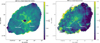 |
Fig. 2 Spectral index maps of the Crab Nebula at low radio frequencies. Left: spectral index map between 54 MHz and 1520 MHz, with an angular resolution of 11″. Right: spectral index map between 145 MHz and 1520 MHz, with an angular resolution of 0.8″. |
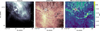 |
Fig. 3 Cutout of the filament with a flat spectral index visible in the HBA to L band (145 MHz to 1.5 GHz) spectral index map (‘Filament 1’). On the left is the region as seen in the Chandra Low-Energy Transmission Grating with the High-Resolution Camera Spectroscopy detector (Weisskopf et al. 2012), in the middle as seen in the LOFAR HBA at 145 MHz, and in the right, the HBA to L band (145 MHz to 1.5 GHz) spectral index map (same as Fig. 2, right). The contours correspond to spectral index values of α = −0.15 and 0.05. |
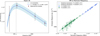 |
Fig. 4 Left: example of the best-fit procedure for a given region (Region 48 as labelled in Fig. 5). The data points are the integrated flux density measurements for the region in each of the images. We fit for the values of S0 and X in Eq. (4), and then convert to a best-fit value of EM with its associated error after fixing, in this case T = 20 000 K and Z = 3. This is the same procedure that is followed on a pixel-by-pixel basis when making Figs. 6 and 7. The turnover frequency (νt) in this case occurs at 130 MHz and is indicated by the vertical dashed line. Right: emission measure (EM) as a function of turnover frequency (νturnover) for the regions labelled in Fig. 5. The values in green correspond to the regions in Table 3, and the values in blue to those in Table 2. The dashed lines are the analytical relationship between EM and νturnover for the corresponding values of T and Z. |
3.3 Electron density in the Rayleigh–Taylor filaments
Ideally, we would use the best-fit values of Fig. 5 alongside Eqs. (2) and (3) to obtain a value for the emission measure (EM) and electron number density (ne) in the absorbing filaments. This requires knowing the average temperature (T) and charge (Z) of the absorbing material. Note that the neutral atoms, the molecules, and the dust present in the filaments (Graham et al. 1990; Sankrit et al. 1998; Temim et al. 2024) do not contribute to the low frequency absorption that this method is sensitive to (since free-free absorption requires free electrons).
A further necessary parameter is the thickness of the absorbing volume. Filament 1 appears to have a clumpy structure (see Fig. 3), but we measure its average width to be 3″. In the low-resolution map, we are sensitive to thicker (yet in some cases resolved) structures; for the same Filament 1 we measure an average width of 15″. Here we approximated the length of the absorbing slab l in Eq. (3) as the measured thickness of the filaments.
Fesen & Kirshner (1982) present spectroscopic observations of several filaments in the Crab Nebula, and find electron temperatures in the range 11 000-18 300 K and a typical electron density in the filaments of 1300 cm−3. Using Z = 2, T = 15 000 K, and a filament thickness of l = 3″ (0.03 pc for a 2 kpc distance to the Crab; Trimble 1973), the resulting ne values are in good agreement with those of Fesen & Kirshner (1982): the densest knot has ne = 1410 ± 140 cm−3 at its highest value (α = 5h34m29s.1, δ = +22°00′36.6″) and the filaments show ne = 600–800 cm−3 in their more diffuse parts (see Fig. 6).
We also measured the flux density in a series of regions (shown in Fig. 5, left) in each of the images and jointly fitted for the absorption for their average values of EM and ne. In Table 2, we show the best-fit values for EMZ=2,T=15 000 and ne l=0.03), where
![Mathematical equation: $\[E M(Z, T)=E M_{Z=2, T=15~000}\left(\frac{3}{Z}\right)\left(\frac{T}{20~000 \mathrm{~K}}\right)^{3 / 2}\]$](/articles/aa/full_html/2025/07/aa55333-25/aa55333-25-eq5.png) (5)
(5)
and
![Mathematical equation: $\[n_e(Z, T, l)=n_{e ~l=0.03}\left(\frac{2}{Z}\right)^{1 / 2}\left(\frac{T}{15~000 \mathrm{~K}}\right)^{3 / 4}\left(\frac{0.03 ~\mathrm{pc}}{l}\right)^{1 / 2}.\]$](/articles/aa/full_html/2025/07/aa55333-25/aa55333-25-eq6.png) (6)
(6)
Carrying out a similar analysis using the low-resolution best-fit maps (which include the LOFAR LBA data at 54 MHz) the effects of absorption are visible at scales that are partially resolved in some cases, indicating a larger absorbing volume. As seen in Fig. 5, right, the region of most intense absorption is thicker than the angular resolution of the LBA map, with an approximate width of 15″ and measuring over 20″ at its thickest point. However, many of the features are only as wide as the angular resolution of the LBA map, implying that their thickness should be less than 0.08 pc.
We do not know the average T and Z values in the volume probed by the LOFAR LBA observations, but from the stratified ionisation structure of the filaments it is clear that both Z and T should be higher than the values we used for the high-resolution analysis. Using Z = 3 and T = 20 000 and a filament thickness of l = 8″ (0.075 pc) the resulting ne are in the range of ~50–250 cm−3, (see Fig. 7). For a series of regions shown in Fig. 5, right, we show the best-fit values of EMZ=3,T=20 000 and ne l = 0.08, defined as above, in Table 3. The flux density values and best-fit parameters for a sample region showing high absorption are plotted in Fig. 4, right. Note that for the region 46 (corresponding to Filament 1), which is resolved, the value of ne is slightly overestimated, as a more appropriate value of l for this region is l ~ 0.15 pc.
Finally, in Tables 2 and 3 we show the turnover frequency vturover corresponding to the peak of the spectrum of each region for the best-fit values of the parameters. The turnover frequency is obtained directly from fitting Eq. (4) to the parameters. Figure 4, right, shows a plot of the emission measure as a function of turnover frequency for the regions under consideration.
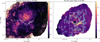 |
Fig. 5 Left: best-fit free-free optical depth at 145 MHz. The integrated values for the regions labelled 1–14 are shown in Table 2. Right: best-fit free-free optical depth at 54 MHz. The integrated values for the regions labelled 21–70 are shown in Table 3. The region within the white box corresponds to the inset plotted in Fig. 7. |
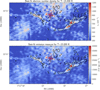 |
Fig. 6 Results from combining our best-fit absorption values with Eqs. (2) and (3) using T = 15 000 K (Fesen & Kirshner 1982), Z = 2, and l = 0.03 pc. Plotted are the electron number density (ne; above) and emission measure (EM; below). The contours correspond to the blueshifted oxygen emission as mapped in Martin et al. (2021). Note that the contour levels are the same in Fig. 7. |
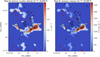 |
Fig. 7 Results from combining our best-fit absorption values with Eqs. (2) and (3) using T = 20 000 K (Fesen & Kirshner 1982), Z = 3, and l = 0.08 pc. Plotted are the electron number density (ne; left) and emission measure (EM; right). The region displayed here is shown as a blue box in Fig. 5, middle. The contours correspond to the blueshifted oxygen emission as mapped in Martin et al. (2021). Note that the contour levels are the same in Fig. 6. |
3.4 Non-detection of the supernova remnant shell
The supernova blast wave is not visible as an extended outer shell in the case of the Crab Nebula, unlike for other young supernova remnants. Sollerman et al. (2000) found evidence of a fast outer shell surrounding the visible nebula from the far ultraviolet spectrum of the pulsar; they inferred a mass and velocity in the extended shell of 0.3 M⊙ and 2500 km s−1, respectively.
We made a lower-resolution image in the HBA band with a minimum baseline length of 80λ, sensitive to structures of up to 43′, and could not find evidence of a radio shell around the Crab. At a distance of 2 kpc (Trimble 1973), 43′ corresponds to a physical length of 25 pc; for reference, if the blast wave had a free expansion velocity of 10 000 km s−1 for 1000 years, the resulting structure would have a radius of 10 pc (17′).
At the edge of the low-resolution map, 25′ away from the pulsar, the noise is 4 mJy bm−1 for a 6″ × 8″ beam, corresponding to a surface brightness upper limit of Σ = 3.5 × 10⁻²⁰ W m−2 Hz−1 sr−1; the noise of the map increases as we move closer to the nebula. This is a less stringent upper limit than the one quoted for the Crab shell by Frail et al. (1995) from VLA 330 MHz data due to the dynamic range limitations posed by the Crab pulsar, for which we measure a spectral index as steep as α ~ −3 between 145 and the 1520 MHz maps.
4 Discussion
The absorption effects visible in our analysis are associated with features in the optical and infrared that trace the densest material in the filaments. Comparing the dust and [S III] emission in Fig. 10 of Temim et al. (2024) with the location of our regions plotted in Fig. 5 and Tables 2 and 3, we can see that all the regions, both in the high and low resolution maps, have a bright counterpart in these components.
It is not straightforward to go from a measurement of the optical depth (which our observations are sensitive to) to physically meaningful quantities describing the plasma. Conclusions about the electron densities in the free-free absorbing material are dependent on its ionisation state and temperature structures. But, as with most astronomical objects, the more high resolution observations are available, the more complex the source appears; in the case of the Crab Nebula, the clearer it becomes that a variety of compositions and ionisation states are present in a given filament, and that the filaments sustain a range of temperatures. This became evident once the Hubble Space Telescope first observed the cage of filaments in the nebula (Sankrit et al. 1998), and the complexity of their structure was further revealed by the James Webb Space Telescope (Temim et al. 2024).
Sankrit et al. (1998) found that the filaments in the Crab show neutral and low-ionisation emission concentrated in sharp structures, and high-ionisation emission occurring in a more diffuse component. This is similar to what we find by comparing the high and low resolution maps: the absorption at 54 MHz is more extended, and overlaps with the majority of the optical foreground (blueshifted) filaments, whereas the absorption visible in the 145 MHz map is limited to the one filament that traverses the nebula south of the pulsar, Filament 1 (seen in Fig. 6). The difference is due to the fact that the high resolution map is only sensitive to structures for which the turnover frequency due to free-free absorption happens at a frequency higher than the LOFAR HBA observations at 145 MHz, which requires an overall higher density and/or lower temperature than a turnover at ≳50 MHz, which the low-resolution map is sensitive to. The regions in high resolution map that we fitted for have ne l = 0.03 in the 500–1000 cm−3 range (although this is due to integrating over an area; the map in Fig. 6 shows that for the hotspots the electron density is >1000 cm−3), whereas the low-resolution regions have ne l=0.08 ≈ 100–200 cm−3.
Sankrit et al. (1998) modelled the photoionisation structure of the filaments with lower temperatures (4000–9000 K) for the innermost filament; this is less than the value we assumed to make Fig. 6 (15 000 K). However, the core of the filaments for which these temperatures are valid has a scale ~1016 cm, whereas for the high-resolution map, our method is only tracking scales of ~1018 cm.
Our absorption study finds that this density stratification extends to much larger scales than the ones considered by Sankrit et al. (1998). Whereas it is the case that many of the regions fitted for in Table 3 have widths of the order of the angular resolution of the LOFAR LBA map, this is not the case for the highly absorbed filament labelled Filament 1, which is partially resolved. Comparing Figs. 6 and 7 it is clear that the region of high emission measure is more extended in the low-resolution map (it extends further along the western side). Both components are visible within the oxygen contours, but the highest absorption at high frequencies coincides with the brightest optical emission, whereas the highest absorption values in the low-resolution map coincide with a region of more extended and fainter optical emission.
Whereas the absorbed filament in the high-resolution map is resolved, and has a thickness of ~0.03 pc, in most cases, the filaments visible in the low-resolution map are unresolved in their width dimension, implying that they are in general <0.08 pc. However, at its thickest, the region of high optical depth at 54 MHz is ~0.2 pc. It is not possible to tell whether this is due to an overlap of thinner filaments as opposed to an extended envelope, although if this were the case, we would expect to see their structure in the high-resolution map. The lack of features in the optical depth map at 145 MHz points to the ~0.2 pc structure being indeed an extended region of relatively low density.
5 Summary and conclusions
We made a sub-arcsecond angular resolution map of the Crab Nebula at 145 MHz by re-processing LoTSS observations to include the LOFAR international stations. These are the highest-angular-resolution low-frequency observations of the source to date.
Combining this map with archival observations at 5 GHz, 1.5 GHz, and 54 MHz, we fitted for free-free absorption due to ionised material in front of the synchrotron nebula. Our absorption fit recovered the morphology of the cage of thermally emitting filaments composed of stellar ejecta that surround the pulsar wind nebula, indicating that they are the source of absorption. The inclusion or not of the 54 MHz map in the fit (whose resolution is much lower than the remaining three maps but which is much more sensitive to the effects of absorption) resulted in two different optical depth maps, sensitive to two different filamentary components: a compact component, resolved, with a thickness of ~0.03 pc and electron densities of 500–1200 cm−3, and a more extended component enveloping the dense component, with electron densities <200 cm−3. The width of this second component varies, with structures that could well be <0.08 pc and structures as large as 0.2 pc. These findings suggest that the well-known stratified density, temperature and ionisation structure of the Crab Nebula’s optical filaments might extend to larger scales than previously considered.
Data availability
The 145 and 1520 MHz maps are available at the CDS via anonymous ftp to cdsarc.cds.unistra.fr (130.79.128.5) or via https://cdsarc.cds.unistra.fr/viz-bin/cat/J/A+A/699/A319.
Acknowledgements
We thank M. Bietenholz for sharing his VLA 5 GHz map of the Crab. We thank D. Milisavljevic and Z. Ding for sharing their optical data, and J. Vink for our helpful scientific discussions on the Crab Nebula. We also thank the anonymous referee for their useful comments, which improved the paper. MA acknowledges support from the VENI research programme with project number 202.143, which is financed by the Netherlands Organisation for Scientific Research (NWO). RT is grateful for support from the UKRI Future Leaders Fellowship (grant MR/T042842/1). This work was supported by the STFC [grants ST/T000244/1, ST/V002406/1]. FS appreciates the support of STFC [ST/Y004159/1]. LOFAR (van Haarlem et al. 2013) is the LOw Frequency ARray designed and constructed by ASTRON. It has observing, data processing, and data storage facilities in several countries, which are owned by various parties (each with their own funding sources), and are collectively operated by the ILT foundation under a joint scientific policy. The ILT resources have benefited from the following recent major funding sources: CNRS-INSU, Observatoire de Paris and Université d’Orléans, France; BMBF, MIWF-NRW, MPG, Germany; Science Foundation Ireland (SFI), Department of Business, Enterprise and Innovation (DBEI), Ireland; NWO, The Netherlands; The Science and Technology Facilities Council, UK; Ministry of Science and Higher Education, Poland; Istituto Nazionale di Astrofisica (INAF), Italy. This research made use of the Dutch national e-infrastructure with support of the SURF Cooperative (e-infra 180169) and the LOFAR e-infra group. The Jülich LOFAR Long Term Archive and the German LOFAR network are both coordinated and operated by the Jülich Supercomputing Centre (JSC), and computing resources on the supercomputer JUWELS at JSC were provided by the Gauss Centre for Supercomputing e.V. (grant CHTB00) through the John von Neumann Institute for Computing (NIC). This research made use of the University of Hertfordshire high-performance computing facility and the LOFAR-UK computing facility located at the University of Hertfordshire and supported by STFC [ST/P000096/1], and of the Italian LOFAR IT computing infrastructure supported and operated by INAF, and by the Physics Department of Turin University (under an agreement with Consorzio Interuniversitario per la Fisica Spaziale) at the C3S Supercomputing Centre, Italy.
References
- Arias, M., Vink, J., de Gasperin, F., et al. 2018, A&A, 612, A110 [NASA ADS] [CrossRef] [EDP Sciences] [Google Scholar]
- Arias, M., Vink, J., Zhou, P., et al. 2019, AJ, 158, 253 [NASA ADS] [CrossRef] [Google Scholar]
- Baars, J. W. M., Genzel, R., Pauliny-Toth, I. I. K., & Witzel, A. 1977, A&A, 61, 99 [NASA ADS] [Google Scholar]
- Bietenholz, M. F., & Kronberg, P. P. 1990, ApJ, 357, L13 [NASA ADS] [CrossRef] [Google Scholar]
- Bietenholz, M. F., Kassim, N., Frail, D. A., et al. 1997, ApJ, 490, 291 [NASA ADS] [CrossRef] [Google Scholar]
- Bietenholz, M. F., Hester, J. J., Frail, D. A., & Bartel, N. 2004, ApJ, 615, 794 [NASA ADS] [CrossRef] [Google Scholar]
- Bietenholz, M. F., Yuan, Y., Buehler, R., Lobanov, A. P., & Blandford, R. 2015, MNRAS, 446, 205 [NASA ADS] [CrossRef] [Google Scholar]
- Blair, W. P., Long, K. S., Vancura, O., et al. 1992, ApJ, 399, 611 [NASA ADS] [CrossRef] [Google Scholar]
- Chevalier, R. A., & Gull, T. R. 1975, ApJ, 200, 399 [Google Scholar]
- de Gasperin, F., Dijkema, T. J., Drabent, A., et al. 2019, A&A, 622, A5 [NASA ADS] [CrossRef] [EDP Sciences] [Google Scholar]
- de Gasperin, F., Vink, J., McKean, J. P., et al. 2020, A&A, 635, A150 [NASA ADS] [CrossRef] [EDP Sciences] [Google Scholar]
- Fesen, R. A., & Kirshner, R. P. 1982, ApJ, 258, 1 [Google Scholar]
- Frail, D. A., Kassim, N. E., Cornwell, T. J., & Goss, W. M. 1995, ApJ, 454, L129 [Google Scholar]
- Graham, J. R., Wright, G. S., & Longmore, A. J. 1990, ApJ, 352, 172 [Google Scholar]
- Heiles, C., & Campbell, D. B. 1970, Nature, 226, 529 [Google Scholar]
- Hester, J. J. 2008, ARA&A, 46, 127 [Google Scholar]
- Hester, J. J., Stone, J. M., Scowen, P. A., et al. 1996, ApJ, 456, 225 [Google Scholar]
- Intema, H. T., Jagannathan, P., Mooley, K. P., & Frail, D. A. 2017, A&A, 598, A78 [NASA ADS] [CrossRef] [EDP Sciences] [Google Scholar]
- Karuppusamy, R., Stappers, B. W., & van Straten, W. 2010, A&A, 515, A36 [NASA ADS] [CrossRef] [EDP Sciences] [Google Scholar]
- Kassim, N. E., Perley, R. A., Erickson, W. C., & Dwarakanath, K. S. 1993, AJ, 106, 2218 [Google Scholar]
- Kent, B. R., Masters, J. S., Chandler, C. J., et al. 2018, in American Astronomical Society Meeting Abstracts, 231, 342.14 [Google Scholar]
- Loll, A. M., Desch, S. J., Scowen, P. A., & Foy, J. P. 2013, ApJ, 765, 152 [Google Scholar]
- Martin, T., Milisavljevic, D., & Drissen, L. 2021, MNRAS, 502, 1864 [NASA ADS] [CrossRef] [Google Scholar]
- Morabito, L., Jackson, N., Mooney, S., et al. 2022, A&A, 658, A1 [NASA ADS] [CrossRef] [EDP Sciences] [Google Scholar]
- Offringa, A. R., McKinley, B., Hurley-Walker, N., et al. 2014, MNRAS, 444, 606 [Google Scholar]
- Owen, P. J., & Barlow, M. J. 2015, ApJ, 801, 141 [NASA ADS] [CrossRef] [Google Scholar]
- Rybicki, G. B., & Lightman, A. P. 1986, Radiative Processes in Astrophysics (Wiley-VCH) [Google Scholar]
- Sankrit, R., Hester, J. J., Scowen, P. A., et al. 1998, ApJ, 504, 344 [Google Scholar]
- Shimwell, T. W., Röttgering, H. J. A., Best, P. N., et al. 2017, A&A, 598, A104 [NASA ADS] [CrossRef] [EDP Sciences] [Google Scholar]
- Shimwell, T. W., Tasse, C., Hardcastle, M. J., et al. 2019, A&A, 622, A1 [NASA ADS] [CrossRef] [EDP Sciences] [Google Scholar]
- Shimwell, T. W., Hardcastle, M. J., Tasse, C., et al. 2022, A&A, 659, A1 [NASA ADS] [CrossRef] [EDP Sciences] [Google Scholar]
- Sollerman, J., Lundqvist, P., Lindler, D., et al. 2000, ApJ, 537, 861 [Google Scholar]
- Temim, T., Laming, J. M., Kavanagh, P. J., et al. 2024, ApJ, 968, L18 [Google Scholar]
- Trimble, V. 1973, PASP, 85, 579 [NASA ADS] [CrossRef] [Google Scholar]
- van Haarlem, M. P., Wise, M. W., Gunst, A. W., et al. 2013, A&A, 556, A2 [NASA ADS] [CrossRef] [EDP Sciences] [Google Scholar]
- van Weeren, R. J., Williams, W. L., Hardcastle, M. J., et al. 2016, ApJS, 223, 2 [Google Scholar]
- van Weeren, R. J., Shimwell, T. W., Botteon, A., et al. 2021, A&A, 651, A115 [NASA ADS] [CrossRef] [EDP Sciences] [Google Scholar]
- Weisskopf, M. C., Elsner, R. F., Kolodziejczak, J. J., O’Dell, S. L., & Tennant, A. F. 2012, ApJ, 746, 41 [NASA ADS] [CrossRef] [Google Scholar]
- Williams, W. L., van Weeren, R. J., Röttgering, H. J. A., et al. 2016, MNRAS, 460, 2385 [Google Scholar]
The dependence, for constant T and Z, is found by setting the derivative of Eq. (1) to zero and solving numerically for v. Note that νturnover ≈ ντ=1, the value of v for which the optical depth is equal to one.
All Tables
All Figures
|
Fig. 1 The Crab Nebula as seen with the HBA of the ILT. This map has a central frequency of 145 MHz, an angular resolution of 0.43″ × 0.28″, an rms noise of 260 μJy bm−1, and a dynamic range of 61 000; the area displayed here has a size of 8′ × 8′. |
| In the text | |
|
Fig. 2 Spectral index maps of the Crab Nebula at low radio frequencies. Left: spectral index map between 54 MHz and 1520 MHz, with an angular resolution of 11″. Right: spectral index map between 145 MHz and 1520 MHz, with an angular resolution of 0.8″. |
| In the text | |
|
Fig. 3 Cutout of the filament with a flat spectral index visible in the HBA to L band (145 MHz to 1.5 GHz) spectral index map (‘Filament 1’). On the left is the region as seen in the Chandra Low-Energy Transmission Grating with the High-Resolution Camera Spectroscopy detector (Weisskopf et al. 2012), in the middle as seen in the LOFAR HBA at 145 MHz, and in the right, the HBA to L band (145 MHz to 1.5 GHz) spectral index map (same as Fig. 2, right). The contours correspond to spectral index values of α = −0.15 and 0.05. |
| In the text | |
|
Fig. 4 Left: example of the best-fit procedure for a given region (Region 48 as labelled in Fig. 5). The data points are the integrated flux density measurements for the region in each of the images. We fit for the values of S0 and X in Eq. (4), and then convert to a best-fit value of EM with its associated error after fixing, in this case T = 20 000 K and Z = 3. This is the same procedure that is followed on a pixel-by-pixel basis when making Figs. 6 and 7. The turnover frequency (νt) in this case occurs at 130 MHz and is indicated by the vertical dashed line. Right: emission measure (EM) as a function of turnover frequency (νturnover) for the regions labelled in Fig. 5. The values in green correspond to the regions in Table 3, and the values in blue to those in Table 2. The dashed lines are the analytical relationship between EM and νturnover for the corresponding values of T and Z. |
| In the text | |
|
Fig. 5 Left: best-fit free-free optical depth at 145 MHz. The integrated values for the regions labelled 1–14 are shown in Table 2. Right: best-fit free-free optical depth at 54 MHz. The integrated values for the regions labelled 21–70 are shown in Table 3. The region within the white box corresponds to the inset plotted in Fig. 7. |
| In the text | |
|
Fig. 6 Results from combining our best-fit absorption values with Eqs. (2) and (3) using T = 15 000 K (Fesen & Kirshner 1982), Z = 2, and l = 0.03 pc. Plotted are the electron number density (ne; above) and emission measure (EM; below). The contours correspond to the blueshifted oxygen emission as mapped in Martin et al. (2021). Note that the contour levels are the same in Fig. 7. |
| In the text | |
|
Fig. 7 Results from combining our best-fit absorption values with Eqs. (2) and (3) using T = 20 000 K (Fesen & Kirshner 1982), Z = 3, and l = 0.08 pc. Plotted are the electron number density (ne; left) and emission measure (EM; right). The region displayed here is shown as a blue box in Fig. 5, middle. The contours correspond to the blueshifted oxygen emission as mapped in Martin et al. (2021). Note that the contour levels are the same in Fig. 6. |
| In the text | |
Current usage metrics show cumulative count of Article Views (full-text article views including HTML views, PDF and ePub downloads, according to the available data) and Abstracts Views on Vision4Press platform.
Data correspond to usage on the plateform after 2015. The current usage metrics is available 48-96 hours after online publication and is updated daily on week days.
Initial download of the metrics may take a while.