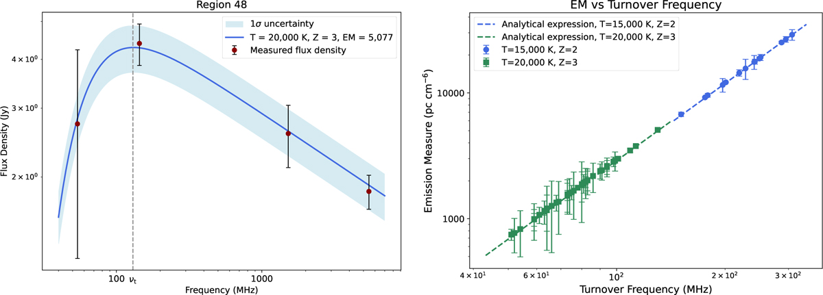
Left: example of the best-fit procedure for a given region (Region 48 as labelled in Fig. 5). The data points are the integrated flux density measurements for the region in each of the images. We fit for the values of S₀ and X in Eq. (4), and then convert to a best-fit value of EM with its associated error after fixing, in this case T = 20 000 K and Z = 3. This is the same procedure that is followed on a pixel-by-pixel basis when making Figs. 6 and 7. The turnover frequency (ν_t) in this case occurs at 130 MHz and is indicated by the vertical dashed line. Right: emission measure (EM) as a function of turnover frequency (ν_turnover) for the regions labelled in Fig. 5. The values in green correspond to the regions in Table 3, and the values in blue to those in Table 2. The dashed lines are the analytical relationship between EM and ν_turnover for the corresponding values of T and Z.