| Issue |
A&A
Volume 699, July 2025
|
|
|---|---|---|
| Article Number | A354 | |
| Number of page(s) | 11 | |
| Section | Interstellar and circumstellar matter | |
| DOI | https://doi.org/10.1051/0004-6361/202555308 | |
| Published online | 22 July 2025 | |
The HI-to-H2 transition in the Draco cloud
1
I. Physikalisches Institut, Universität zu Köln,
Zülpicher Str. 77,
50937
Köln,
Germany
2
Physikalischer Verein, Gesellschaft für Bildung und Wissenschaft,
Robert-Mayer-Str. 2,
60325
Frankfurt,
Germany
3
Universität Heidelberg, Zentrum für Astronomie,
69120
Heidelberg,
Germany
4
Physics Department, University of California,
San Diego, La Jolla,
CA
92093-0319,
USA
5
SOFIA Science Center, NASA Ames Research Center,
Moffett Field,
CA
94 045,
USA
★ Corresponding author: nschneid@ph1.uni-koeln.de
Received:
26
April
2025
Accepted:
24
June
2025
In recent decades, significant attention has been dedicated to analytical and observational studies of the atomic hydrogen (H I) to molecular hydrogen (H2) transition in the interstellar medium. We focussed on the Draco diffuse cloud to gain deeper insights into the physical properties of the transition from H I to H2. We employed the total hydrogen column density probability distribution function (N-PDF) derived from Herschel dust observations and the NHI-PDF obtained from H I data collected by the Effelsberg H I survey. The N-PDF of the Draco cloud exhibits a double-log-normal distribution, whereas the NHI-PDF follows a single log-normal distribution. The H I-to-H2 transition is identified as the point where the two log-normal components of the dust N-PDF contribute equally; it occurs at AV ~ 0.33 (N ~ 6.2 × 1020 cm−2). The low-column-density segment of the dust N-PDF corresponds to the cold neutral medium, which is characterized by a temperature of around 100 K. The higher-column-density part is predominantly associated with H2. The shape of the Draco N-PDF is qualitatively reproduced by numerical simulations. In the absence of substantial stellar feedback, such as radiation or stellar winds, turbulence exerts a significant influence on the thermal stability of the gas and can regulate the condensation of gas into denser regions and its subsequent evaporation. Recent observations of the ionized carbon line at 158 μm in Draco support this scenario. Using the KOSMA-tau photodissociation model, we estimate a gas density of n ~50 cm−3 and a temperature of ~100 K at the location of the H I-to-H2 transition. Both the molecular and atomic gas components are characterized by supersonic turbulence and strong mixing, suggesting that simplified steady-state chemical models are not applicable under these conditions.
Key words: ISM: clouds / dust, extinction / ISM: structure
© The Authors 2025
 Open Access article, published by EDP Sciences, under the terms of the Creative Commons Attribution License (https://creativecommons.org/licenses/by/4.0), which permits unrestricted use, distribution, and reproduction in any medium, provided the original work is properly cited.
This article is published in open access under the Subscribe to Open model. Subscribe to A&A to support open access publication.
1 Introduction
The formation of molecular hydrogen (H2) in the interstellar medium (ISM) has historically been described using steadystate and chemical equilibrium models (Tielens & Hollenbach 1985; van Dishoeck & Black 1988; Sternberg & Dalgarno 1989; Krumholz et al. 2008). In such models, the dissociation of H2 by photons in the Lyman-Werner bands from the local radiation field competes with H2 formation on the surfaces of dust grains. Although H2 self-shielding and dust shielding against UV photodissociation are highly effective, the formation rate of molecular H2 remains relatively low, approximately 3 × 10⁻¹⁷ cm3 s−1 (Jura 1974). The H2 formation rate and the efficiency of dust shielding are further influenced by the abundance of dust grains, which is commonly scaled in models based on metallicity. For a more detailed discussion of the atomic-to-molecular hydrogen (H i-to-H2) transition and associated references, see Bellomi et al. (2020) and Park et al. (2023). In dynamic scenarios, however, H2 formation is also influenced by turbulent mixing motions in the ISM (Glover & Mac Low 2007; Bialy et al. 2017). These motions induce large- and small-scale density fluctuations that can drastically reduce H2 formation timescales from tens of millions of years to just a few million years (Glover & Mac Low 2007; Valdivia et al. 2016). This reduction in timescales has profound implications for the ISM. For instance, Mac Low & Glover (2012) argue that star-forming clouds are often disrupted by stellar feedback before they can reach chemical equilibrium.
Turbulence in the ISM can be generated by a variety of mechanisms. These include colliding H i flows and other dynamic processes that lead to H2 formation in shock-compressed layers (Walder & Folini 1998; Koyama & Inutsuka 2000; Heitsch et al. 2006; Vázquez-Semadeni et al. 2006; Dobbs 2008; Hennebelle et al. 2008; Banerjee et al. 2009; Clark et al. 2012; Colman et al. 2025). Additionally, large-scale gravitational instabilities in the galactic disc and stellar feedback, predominantly from supernova explosions, contribute significantly to turbulence generation (Mac Low & Klessen 2004; Klessen & Glover 2016).
In plane-parallel photodissociation region (PDR) models (van Dishoeck & Black 1986; Hollenbach et al. 1991; Wolfire et al. 2010; Sternberg et al. 2014), the H i-to-H2 transition is parameterized by the density of the gas and the intensity of the incident radiation field. For low densities (typically n < 103 cm−3) and a weak to moderate far-ultraviolet (FUV) radiation field1, with χ in the range 1-103, the H i-to-H2 transition occurs at visual extinctions (AV) below unity2. Due to molecular formation and the cumulative dust shielding, this transition is accompanied by a significant drop in temperature, typically from values exceeding 100 K to approximately 20 K. Imara & Burkhart (2016) observed a column density of NH ~ 8-20 × 1020 cm−2 (AV ~ 0.4-1.1) for the Hi-to-H2 transition in optically thick molecular clouds surrounded by H i envelopes. Studies of infrared cirrus, as well as intermediate-velocity clouds (IVCs) and high-velocity clouds (HVCs: Reach et al. 1994; Lagache et al. 1998; Gillmon et al. 2006; Gillmon & Shull 2006; Röhser et al. 2014), suggest values of NH ~ 2-5 × 1020 cm−2 (AV−0.1-0.3) for the H I-to-H2 transition. Similar values were found by Schneider et al. (2022) using column density probability distribution functions (N-PDFs) of dust for diffuse, quiescent, and low-density clouds. Moreover, the H i to far-infrared (FIR) continuum relation turns non-linear at values above NH = 5 × 1020 cm−2 (Desert et al. 1988; Lenz et al. 2015; Planck Collaboration 2011), which is interpreted as the transition from atomic to molecular hydrogen.
While the chemical state of the ISM is governed by the balance between photodissociation and H2 formation on dust grains, its thermal state is regulated by heating processes, such as the photoelectric effect, and cooling, primarily through collisionally excited emission in FIR molecular and atomic fine-structure lines. The relatively shallow dependence of the cooling rate on temperature for T < 104 K, dominated by cooling via the ionized carbon [C ii] 158 μm line, leads to thermal instabilities that produce a multi-phase ISM (Field et al. 1969; Wolfire et al. 1995). It consists of volume-filling warm neutral medium (WNM), characterized by temperatures of T - 8000 K and densities n ~ 1 cm−3, in pressure equilibrium with the cold neutral medium (CNM), which has temperatures of T ~ 30-100 K and densities n ~ 10-100 cm−3 (Wolfire et al. 2003; Bialy & Sternberg 2019). Additionally, molecular H2 gas typically exhibits temperatures below 30 K and densities exceeding several hundred cm−3. However, thermally unstable gas, often referred to as the lukewarm neutral medium or the unstable neutral medium (UNM; Murray et al. 2018), can also exist with temperatures in between those of the CNM and the WNM (Marchal et al. 2019). Depending on its density, such gas can cool to become denser and fully molecular, or it can heat up and join the WNM (Heiles & Troland 2003). Under turbulent conditions, significant amounts of thermally unstable gas can be present as turbulent motions expand the interface between stable thermal phases. Although this unstable gas is challenging to observe, it plays a critical role in probing the H i-to-H2 transition as a function of the hydrogen column density and the incident UV field, offering insights into the formation of molecular clouds and stars from diffuse H i gas. A possible tracer of this gas phase is the [C ii] line, as proposed by Schneider et al. (2023), who observed interacting flows - partly atomic, partly molecular - in the Cygnus X region. This gas, which does not emit prominently in the lines of carbon monoxide and is thus called ‘CO-dark’ (Wolfire et al. 2010), has a density of n ~ 100 cm−3 at T - 100 K in Cygnus.
To investigate the H i-to-H2 transition, we selected the Draco iVC, a region that is likely on the verge of forming a molecular cloud and is exposed to a very low incident UV field. The dust column density map of this high-latitude cloud was obtained from FiR dust continuum maps based on observations taken with the Herschel satellite and was presented in Schneider et al. (2022, 2024). This map, which spans a large dynamic range, includes both atomic and molecular phases, with the relative contributions of these phases depending on the cloud’s evolutionary state. Other column density maps of Draco at various angular resolutions obtained from Herschel were created by Miville-Deschênes et al. (2017) and Bieging & Kong (2024). in Schneider et al. (2022) we demonstrate that the atomic and molecular gas in Draco can be separated using N-PDFs. For the atomic N-PDF, we utilized H i data from the Effelsberg H i survey (Winkel et al. 2016), with an angular resolution of 10′. in this study we investigated the physical conditions (e.g. the density and temperature) and dynamics (e.g. the turbulent Mach number) of the atomic and molecular gas. We show that turbulent mixing significantly influences the chemical evolution of clouds and that steady-state equilibrium models fail to explain the observed gas properties.
We start with a short description of the source (Sect. 2) and a summary of the interpretation of the N-PDFs. We then derive the physical properties of the gas using a PDR model, describe its turbulent properties, and compare the observed N-PDF with those obtained from simulations (Sect. 3). Section 4 concludes the paper.
2 The Draco cloud
The Draco cloud (iVC G091.0+38.0, MBM41) is situated above the Galactic plane (Gladders et al. 1998) at a Galactic latitude of b = 38°, corresponding to a scale height of 298 pc, assuming a distance of 481 pc3. Draco is classified as an iVC with a radial velocity of approximately −20 km s−1. it is part of the iR cirrus and is associated with diffuse H i emission (Heiles & Habing 1974). The Draco cloud is thought to originate from a Galactic fountain process, in which material from the Galactic disc is lifted into the halo and subsequently returns to the disc at high velocities (Lenz et al. 2015) and references therein. However, the possibility of infalling extragalactic gas contributing to its origin cannot be entirely ruled out. The Draco iVC is located within the inner Galactic halo and thus outside of the bulk of the WNM in the Galactic disc.
In the HVC part of the region, there is gas with significantly higher negative velocities (v ~ −100 km s−1), and in the low-velocity cloud (LVC) part there are local velocities near 0 km s−1. Figure 1 presents Hi emission channel maps spanning the entire velocity range, from that of the LVC to that of the HVC, alongside a zoomed-in view of the iVC velocity range. Analysis of the low-angular-resolution (10′) Effelsberg-Bonn H i Survey (EBHiS) data reveals the absence of a velocity bridge connecting the HVC and iVC components. Additionally, there is a notable gap in emission around −70 km s−1, meaning there is no clear evidence that Draco originates from a collision between the HVC and iVC, as was previously hypothesized by Herbstmeier et al. (1993). Higher-angular-resolution (1′) data from the Dominion Radio Astrophysical Observatory (DRAO) highlight the small-scale structure of the Draco cloud. At velocities beginning near −13 km s−1, a broad front emerges, characterized by individual knots of emission. At more negative velocities (−19 km s−1), filamentary structures become apparent, oriented towards the Galactic plane. This morphology was interpreted by Kalberla et al. (1984), Rohlfs et al. (1989), and Miville-Deschênes et al. (2017) as indicative of gas compression resulting from a halo cloud interacting with a more diffuse medium as it moves towards the Galactic plane. We note that this paper does not focus on the general physics of iVCs. For further discussion on iVCs, we refer the reader to Putman et al. (2012), Röhser et al. (2014), Röhser et al. (2016a), Röhser et al. (2016b), Kerp et al. (2016), and references therein.
The hydrogen column density map obtained with Herschel is presented in Fig. 2. See Appendix A for further information on this dust column density map. In the regions of highest column density, CO and other molecules with critical densities exceeding 103 cm−3 have been detected (Mebold et al. 1985; Herbstmeier et al. 1993; Schneider et al. 2024). Bieging & Kong (2024) present a 12CO 2→1 map of the whole Draco region at 38″ angular resolution. Comparing our total hydrogen column density map with the CO data (Fig. 2), it becomes obvious that CO is found in the densest regions with a column density around 0.8-1 × 1021 cm−2. These dense clumps consist of molecular hydrogen (H2) and are CO-bright. The remaining emission in the Herschel map is then either CO-dark molecular gas or atomic gas. Note that the CO-bright H2 clumps are also visible in Hi emission, as shown in the right panel of Fig. 1. Bieging & Kong (2024) derived an H2 map by subtracting the DRAO H i map from a total Herschel hydrogen column density map that was obtained using only the 250 μm emission (and not by a spectral energy distribution fit as done in Schneider et al. 2022). With this method, they obtained that CO formation starts at a column density of around 1.3 × 1021 cm−2. Bieging & Kong (2024) estimated that a high fraction of gas in Draco is molecular, in contrast to Schneider et al. (2022), who derived that −89% of the mass in the Draco cloud is composed of atomic hydrogen. Miville-Deschênes et al. (2017), using Herschel dust observations, concluded that the molecular gas primarily consists of small clumps with characteristic sizes of ~0.1 pc, high densities (n ~ 1000 cm−3), and low temperatures (T ~ 20 K). The highly clumpy structure of the gas was confirmed by the CO map of Bieging & Kong (2024). However, the Draco cloud exhibits no evidence of ongoing star formation, as no pre-stellar or protostellar cores have been detected.
Recently, Schneider et al. (2024) reported the first detection of the 158 μm [C ii] line at five positions in the Draco IVC. Combining CO, Hi, and [C ii] data led us to the conclusion that shocks heat the gas that subsequently emit in the [C ii] cooling line. These shocks are probably caused by the motion of the cloud towards the Galactic plane that leads to collisions between H i clouds.
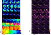 |
Fig. 1 Draco cloud in HI. Left: channel maps of HI brightness temperature in K from EBHIS at 10′ angular resolution in steps of 4 km s−1. The central velocity is given in the lower-left corner, and the individual velocity components of Draco (high, intermediate, and local) are indicated. Right: zoom into the velocity range of the IVC between −12 and −28 km s−1 using the DRAO with the Synthesis Telescope H I data at 1′ angular resolution (Blagrave et al. 2017) in steps of 0.82 km s−1. |
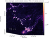 |
Fig. 2 Draco total hydrogen column density map (N(H)) and CO 2→1 contours. The Herschel N(H) map (Schneider et al. 2022, 2024) has an angular resolution of 36″. The 12CO 2→1 data have a resolution of 38″ and stem from Bieging & Kong (2024). The contours are 2, 7, and 12 K km s−1. |
3 Analysis and discussion
In the following analysis, we first determine the physical properties of the gas in the Draco cloud using a PDR model (Sect. 3.1). Subsequently, we examine the turbulent properties of the multiphase gas in Draco (Sect. 3.2) and then compare the observed Draco N-PDF to those obtained from simulations (Sect. 3.3). For this analysis, we utilized the dust and Hi N-PDFs presented in Schneider et al. (2022) and depicted in Fig. B.1. This figure shows a double log-normal PDF for the total hydrogen column density. The lower-column-density component, characterized by a width of σN = 0.32, is attributed to atomic gas, while the higher-column-density component, with a width σN = 0.34, is associated with molecular gas. The H i-to-H2 transition occurs where the contributions from the two log-normal components are equal, corresponding to an extinction value of AV = 0.33 or a column density of NH = 6.2 × 1020 cm−2. Note, however, that H2 can also occur already at lower column densities, but with a lower probability. Bieging & Kong (2024) measured an AV of 0.7 for the onset of CO formation. This value is lower than typical CO formation scale thresholds (Lee et al. 1996; Visser et al. 2009), but well explained if a small-scale clumpy structure of the molecular material is considered with dense clumps of size <0.1 pc. We come back to this point in Sect. 3.1.
Column density PDFs are widely employed as diagnostic tools to characterize the physical processes that shape the column density structure of the ISM. It has been shown that a log-normal density distribution emerges naturally for isothermal flows (e.g. Passot & Vázquez-Semadeni 1998; Vazquez-Semadeni 1994; Padoan et al. 1997; Klessen et al. 2000; Li et al. 2003; Kritsuk et al. 2007; Federrath et al. 2008; Ballesteros-Paredes et al. 2011; Burkhart & Lazarian 2012) and for thermally bistable flows (Audit & Hennebelle 2010; Gazol & Kim 2013), as a result of the central limit theorem. This assumes that density perturbations caused by successive shock passages accumulate independently and randomly.
Previous Herschel studies of evolved star-forming regions have consistently shown a log-normal component in the N-PDF at low column densities. These are often accompanied by one (e.g. Schneider et al. 2013, 2015c,b; Stutz & Kainulainen 2015) or two (Schneider et al. 2015a, 2022) power-law tails at higher column densities, which are typically attributed to the effects of self-gravity (e.g. Kritsuk et al. 2011; Girichidis et al. 2014; Schneider et al. 2015c,b). For example, N-PDFs of the Lupus and Coalsack clouds derived from extinction maps (Kainulainen et al. 2009) appear log-normal in shape. However, Herschel dust-based N-PDFs, which provide a higher dynamic range, reveal a log-normal component at low column densities followed by a power-law tail at higher column densities (Benedettini et al. 2015). Double log-normal N-PDFs with a single powerlaw tail at high column densities were observed by Tremblin et al. (2014) for molecular clouds associated with Hii regions. In these star-forming clouds, the second log-normal component is thought to be produced by feedback processes (Schneider et al. 2022). For Draco, however, no power-law tail is observed, indicating that self-gravity does not yet play a significant role. As said above, this is observationally supported by the nondetection of signposts of ongoing star formation. This suggests that Draco represents an excellent example of a turbulence-dominated, multi-phase region, where the total hydrogen column density is primarily composed of atomic hydrogen.
3.1 Physical properties of the gas
To determine the conditions for the H i-to-H2 transition, we did not try to reproduce the emission and clumpy nature of the Draco cloud but instead performed the simple geometrical study measuring the critical depth for H2 formation in a plane-parallel configuration. The balance between photodissociation of H2 and its formation on dust grain surfaces is controlled by the local gas density and the FUV photon flux.
The FUV radiation field is computed by converting the 160 μm flux observed in Draco into a FUV field assuming that the dust is only heated by FUV radiation (Schneider et al. 2024). This gives a value of χ ~ 1.8-2.5 at the dust peaks4. This is higher than expected as there is no known OB star close to the Draco cloud. In Schneider et al. (2024), we show that cosmic rays are also not a sufficient heating source, which leaves as the most likely reason shock excitation. We assumed an uncertainty of at least a factor of 2 and calculate with an average field of χ ~ 2.
We used the KOSMA-tau PDR model (Röllig et al. 2006, 2007; Röllig & Ossenkopf-Okada 2022) to estimate the average density, 〈n〉, as a function of the incident FUV field and the HI-to-H2 transitional AV. The model is designed to represent clouds by a superposition of spherical clumps with a given mass and density or to model a single clump. Here, n = n(H) + 2n(H2) is the total proton density in cm−3 and 〈〉 indicates the average over the clumps5. In order to approximate a plane-parallel situation in KOSMA-tau, we used a model mass of M = 106 M⊙; this resulted in very large cloud radii. However, the total mass has no significant influence on the H i-to-H2 transition. We computed a grid of model PDRs, covering the diffuse to moderate gas parameter space through gas densities n0 = 1-1000 cm−3 and FUV intensities of χ = 0.1-10. We did not consider turbulent mixing (which is discussed in the next section); we assumed isotropic illumination and expressed our results in terms of AV,eff (Röllig et al. 2007) to be able to convert them from an isotropic illumination to an unidirectional geometry. In Fig. 3, the depth for the transition from H i to H2, i.e. the effective AV at which n(H) = n(H2), is plotted. The general behaviour is intuitive: For a given model density, the transition depth increases with χ. For a fixed FUV strength, the transition occurs at lower AV when the density grows. For the observed transitional H i-to-H2 AV of 0.33 and an UV-field of G0 = 3.4, equivalent to χ = 2, we then derive an average density of 〈n〉 ~ 50 cm−3. This density is consistent with the mean density of 76 cm−3 for cold Hi filament gas at high Galactic latitudes derived by Kalberla (2025). Thus, the scenario we obtain is that small, dense (up to a few times 103 cm−3), cold (T ~ 20 K) molecular cloud clumps are embedded in a lower-density (<50 cm−3) inter-clump medium. An alternative to the steady-state solution computed by KOSMA-tau might be higher densities combined with short timescales. When starting from atomic material, the transition that would occur at AV ~ 0.03 for 〈n〉 = 300 cm−3 in a steady state may well occur at AV ~ 0.3 on the cloud formation timescale, which is too short for the system to reach chemical equilibrium.
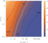 |
Fig. 3 H I-to-H2 transitional AV as a function of UV field and the clump-averaged density 〈n〉, determined from the KOSMA-tau PDR model. The colour wedge gives the value of AV, and the white line indicates our observed transitional AV of 0.33. |
3.2 Turbulence properties of the gas in Draco
Dynamical effects in molecular cloud formation simulations are often neglected and chemistry assumed to be at equilibrium in most of the cases. Exceptions are, for example, the studies of Godard et al. (2014), Valdivia et al. (2016), Seifried et al. (2022), and Ebagezio et al. (2023). Because the dynamical timescale, tdyn, is inverse to the (density-independent) Mach number and the chemical timescale, tchem, for H2 formation on grains is inverse to the density, we are closer to equilibrium when the gas is denser. Because of the relatively low densities in Draco we need to investigate the turbulence properties to assess the importance of dynamical processes in Draco, using the dust PDF (Schneider et al. 2022) and CO observations (Mebold et al. 1985; Herbstmeier et al. 1993; Schneider et al. 2024; Bieging & Kong 2024).
Generally, for a log-normal density (ρ) PDF, the rms sonic Mach number6, M is linked to the standard deviation σρ of the PDF via
 (1)
(1)
The forcing parameter b is related to the kinetic energy injection mechanism and varies from b ≈ 1/3 for solenoidal forcing to b=1 for compressive forcing (Federrath et al. 2008). When magnetic fields are included, the density variance additionally depends on the ratio of thermal pressure pth to magnetic pressure pmag defined as
 (2)
(2)
with the sound speed cs and the Alfvénic velocity, vA. Molina et al. (2012) found that if the magnetic field, B, is proportional to ρ1/2, the density variance is
 (3)
(3)
For N-PDFs, Burkhart & Lazarian (2012) derived the correlation
 (4)
(4)
which does not include any magnetic field dependence. We assumed that the magnetic pressure term scales in a similar fashion as determined by Molina et al. (2012) (Eq. (3)), so
 (5)
(5)
We determined the sonic Mach number MHI for the H I CNM phase from
 (6)
(6)
with the isothermal sound speed cs given as
 (7)
(7)
with the hydrogen mass mH, the Boltzmann constant kB, and the molecular weight μ=1.27.
For Draco, we obtain an average H i linewidth ΔνHI ~ 5 km s−1 from the high-angular-resolution (1′) interferometric DRAO HI data (Blagrave et al. 2017; Schneider et al. 2024). Note, however, that this is a rough approximation. First, there is variation in the line profile with sometimes two components, and second, the line widths for single profiles varies between 4 and 7 km s−1. The temperature is determined in different ways. If we use the PDR toolbox (Pound & Wolfire 2023), with the Wolfire & Kaufman model of 2020 as well as with the KOSMA-tau model from 2020, with a CNM density of 50 cm−3 as an upper limit (Sect. 3.1) and a radiation field of χ ~ 2 (Go ~ 3.4), we obtain a surface temperature of ~100 K. If we use Fig. 2 of Clark et al. (2019), which presents magnetohydrodynamic (MHD) molecular cloud formation simulations, we also obtain a gas temperature of ~ 100 K. Note that such a temperature is on the high end for cold CNM, but still characterize CNM conditions. With T = 100 K and ΔνHI ~ 5 km s−1, we calculate a Mach number of MHI = 4.1. The width (σN) of the dust’s low N-PDF is 0.32 (Fig. B.1), so the b parameter for the hydrodynamic (HD) case is 0.29. If we consider a magnetic field and assume a β of 1, i.e. equipartition between magnetic and thermal pressures, b increases by a factor of  to 0.42. Such a value of the b parameter is consistent with fully developed turbulence. However, it is important to emphasize that the value of b can exhibit significant variation depending on the input parameters used in the calculations. For instance, an increase in the temperature of the CNM or a decrease in the H i line width results in a lower Mach number but a correspondingly higher b-value. Figure 4 illustrates how M and b vary, depending on the H I linewidth and for a range of typical CNM temperatures. From a physical perspective, the b parameter is expected to lie within the range from 0.33 to 1, with a typical value around 0.5. In summary, all reasonable variations within the parameter space defined by line width and temperature lead to supersonic Mach numbers, typically larger than 3, and yield b-values close to 0.5. In all considered scenarios, the flow velocity exceeds the thermal line width, aligning more closely with the relative velocity between the IVC and the LVC.
We calculated the sonic Mach number M for the CO-bright H2 gas phase from
 (8)
(8)
with the CO mass mCO = 28 mH and the mean molecular weight in H2 gas μ = 2.33. We used a temperature of T = 12.5 K for the molecular gas in Draco, which is an average from the COdetermined values shown in Table 8 of Schneider et al. (2024) for a density of a few times 1000 cm−3, consistent with Miville-Deschênes et al. (2017). The typical CO linewidth, ΔvCO, in Draco is 1-1.5 km s−1 for 13CO and 2 km s−1 for 12CO for both the J = 2→1 and 1→0 transitions (Mebold et al. 1985; Herbstmeier et al. 1993; Schneider et al. 2024; Bieging & Kong 2024). We derive a Mach number of M = 6.9 for ΔvCO = 2 km s−1 and M = 5.2 for AvCO = 1.5 km s−1. Note that these values are valid for the CO-bright H2 phase and that M might be somewhat smaller (and b somewhat larger) in the more diffuse CO-dark H2. For the determination of the b parameter, we again used Eqs. (4) and (5) and a width of σN = 0.34 from the Herschel N-PDF for the H2 gas phase. We obtain b = 0.20 (0.27) for ΔvCO = 2 (1.5) km s−1 the HD case and b = 0.28 (0.37) for the magnetized case with β = 1, corresponding to mostly solenoidal driving. If the temperature is higher, the Mach-number is lower and the b parameter increases. However, we note that the CO-linewidth is clearly not lower than 1 km s−1 and shows less variation than the Hi line width.
Summarizing, the cold H i and the H2 gas in Draco are both supersonic, with MHI ~ 4 and MH2 ~ 5. These values are consistent with what was obtained by Miville-Deschênes et al. (2017).
We could then check to what extent the assumption of steady-state chemistry is fulfilled in Draco by calculating the chemical and dynamical timescales, tchem and tdyn, respectively, following Wolfire et al. (2010). In their turbulent scenario, the mass-weighted median density, nmed is defined as
 (9)
(9)
with the Mach number M and the density n. The chemical timescale is then (Wolfire et al. 2010)
 (10)
(10)
which is the time for atomic gas to become completely molecular and R = 3 10−17 cm3 s−1 is the rate coefficient for H2 formation on dust grains assuming solar metallicity (Jura 1974; Gry et al. 2002). For the dynamical time for mixing material over the scale corresponding to an optical depth AV, we used (Wolfire et al. 2010)
![t_{dyn} \, [\mathrm{s}] = \frac{L_{{\rm A}_{\rm V}}}{\sigma} = \frac{1.87 \, 10^{21} \, \cdot {\rm A}_{\rm V}}{10^5 \, n \, \sigma\, [\mathrm{km\,s^{-1}}]}](/articles/aa/full_html/2025/07/aa55308-25/aa55308-25-eq12.png) (11)
(11)
with the 1D velocity dispersion
![\sigma \, [\mathrm{km\,s}^{-1}] = \frac{\Delta {\rm v}\,[\mathrm{km\,s^{-1}}]}{\sqrt{(8 \, \ln(2))}}.](/articles/aa/full_html/2025/07/aa55308-25/aa55308-25-eq13.png) (12)
(12)
This dynamical timescale describes the time needed for the turbulence to mix gas over a length scale LAV corresponding to an optical depth AV to move molecular gas from the dissociation front in a clump to the surface, and to bring atomic gas from the surface to the interior. This scale is then divided by the turbulent velocity field, characterized by σ to obtain tdyn. With M = 4, n = 50 cm−3, AV = 0.33 and Δν = 5 km s−1 (Sect. 3.1), we obtain tdyn = 1.87 Myr. Note that Bieging & Kong (2024) calculated dynamical timescales of individual features in Draco from their CO observations. They obtained that a typical extended clump has a transverse motion of ~ 15′ in 105 yr. For the chemical timescale, following Eq. (10), we estimate tchem = 3.3 Myr. Even considering the uncertainties in all calculations, tchem > tdyn so that dynamical mixing effects cannot be neglected. This estimate shows that it is essential to consider dynamical effects and apply time-dependent chemical models (gas + grains) on observational data.
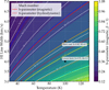 |
Fig. 4 Parameter space for the Mach number and b parameter. The diagram displays the variation in M and b as a function of the H I line width and temperature for the HD case (dotted line) and the magnetic case (straight line). |
3.3 Comparison of the N-PDF to turbulent molecular cloud formation simulations
Various authors performing (M)HD turbulence simulations (Glover & Mac Low 2007; Glover et al. 2010; Micic et al. 2012; Gazol & Kim 2013; Valdivia et al. 2016; Bialy et al. 2017) argue that large density compressions caused by supersonically turbulent gas allow H2 to form more rapidly than in models without turbulence. It was shown that H2 can be rapidly produced on timescales of a few million years and that much of the H2 is formed on very small scales (<0.1 pc) in high-density gas, and then transported to lower densities by turbulent motions. However, there are some subtle differences in the predictions of these studies, which we outline below and compare to our observational results.
Glover & Mac Low (2007) perform turbulent box (size 20 pc) simulations and investigate the H2 formation timescale as a function of density. In their models, the densities must be high in order to obtain a significant H2 fraction. For a density of 50 cm−3 for Draco, we find that 11% of the gas is in molecular form (see also Schneider et al. 2022), consistent with the n = 30 cm−3 case in Glover & Mac Low (2007) with only local shielding (that underestimates the H2 fraction).
Gazol & Kim (2013), Hennebelle & Audit (2007), Seifried et al. (2011), and Valdivia et al. (2016) study thermally bistable turbulent flows. Audit & Hennebelle (2010) in addition compare 2-phase, isothermal and polytropic flows. All authors find double log-normal density and column density PDFs for bistable flows, which is not surprising in view of the bimodal nature of the distribution. Note, however, that the two phases in these studies mostly correspond to WNM and CNM and are thus not directly comparable to what we propose to see in Draco, i.e. the cold atomic and molecular CNM phases. However, Audit & Hennebelle (2010) noticed that their CNM PDF is not well described by a purely log-normal distribution, suggesting that there can be substructure in this part of the PDF; this could correspond to what we observe in Draco. Gazol & Kim (2013) show N-PDFs as a function of Mach number obtained from their purely HD thermally bistable turbulent flows. Again, their N-PDFs are not purely log-normal and their absolute peak values around a few 1020 cm−2 agree with what we observe in Draco. However, it remains unclear which gas phases (WNM or CNM) correspond to which part of their N-PDF.
In order to separate these phases, we calculated the N-PDFs from existing simulations. The first one is a MHD simulation of the multi-phase turbulent ISM (Kritsuk & Norman 2004; Kritsuk et al. 2017) and the second one a 3D zoom-in simulation of the formation of two molecular clouds out of the galactic ISM from the SILCC7-Zoom project (Walch et al. 2015; Girichidis et al. 2016; Seifried et al. 2017). Both simulations include the earliest phases of cloud formation and are thus relevant for the interpretation of the observed N-PDF of Draco. The advantage of these simulations is that it is possible to perform PDFs of total, atomic, and molecular hydrogen individually in different gas phases (CNM, UNM, etc.). We do not expect a one-to-one correspondence since the simulations setup was not designed for the Draco case, but anticipate a qualitative resemblance.
3.3.1 Multi-phase MHD model
The simulation by Kritsuk et al. is a 200 pc multi-phase model with uniform magnetic field strength of B = 3 μG, a mean H i density of5 cm−3, and a velocity dispersion of 16 km s−1. There is no chemistry and no cooling below 18 K in this model, so model-derived temperatures below 18 K may be wrong by a factor of ~2. The density regime is fixed by the mean density of the model, so this should not be expected to make an exact match to the observations. However, the key physics (magnetized multi-phase turbulence) is included and allows for a qualitative comparison to the Draco PDF. The model PDF is shown in Fig. 5. The blue line displays the CNM, the atomic, and molecular phase. This is approximately what can be expected for dust N-PDFs that are not sensitive to the high-temperature WNM. The green line displays the WNM PDF alone with the typical prominent peak at low column densities. This particular simulation already reproduces qualitatively a similar N-PDF (the blue line) as we observed for Draco even though not all observational features match well (PDF width, peak, etc.).
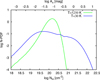 |
Fig. 5 PDF from a MHD simulation (magnetic field strength B = 3μG) of forced multi-phase turbulence (Kritsuk & Norman 2004; Kritsuk et al. 2017) in a 200 pc box with a mean HI density of 5 cm−3 and a velocity dispersion of 16 km s−1. The WNM is represented by the green line, the CNM (atomic and molecular) by the blue line. |
3.3.2 SILCC model
The second model is based on the SILCC-Zoom project that simulates a section of a galactic disc with solar neighbourhood properties and solar metallicity at a size of 500 pc × 500 pc × ±5 kpc. The MHD and purely HD simulations include (supernova-driven) turbulence and self-gravity; they model the chemistry as well as the heating and cooling processes of the ISM using the networks and methods described in Nelson & Langer (1997), Glover & Mac Low (2007), Glover et al. (2010), and Glover & Clark (2012). Various cloud structures develop from the diffuse ISM and are selected for a dedicated high spatial and temporal resolution to study the evolution of their internal substructure and chemistry. From various zoom-in simulations, we selected the HD run using the cloud ‘MC1’ (extent 88 × 78 × 71 pc3 and final mass 7.3 × 10⁴ M) and focus on the early snapshots in the cloud evolution, i.e. 1.5 and 2Myr after the start of the zoom-in procedure. At this time, the H2 fraction of the MC1 cloud is already significant (−50% Seifried et al. 2017), and thus probably more evolved than the Draco cloud8, but still allows for a qualitative comparison to our observations.
Figure 6 shows the resulting PDFs of the total hydrogen column density arising from the CNM and UNM, as we expect for Draco, together with the Draco PDF for comparison. Overall, we observe a good match between the observed and simulated PDFs. The N-PDFs from the simulation also show a double-peak at similar column densities as the Draco N-PDF. As said above, the H2 fraction is slightly higher than in the observed N-PDF, which is not surprising because the MC1 cloud at these two time steps is most likely more evolved as Draco. Only the N-PDF from the simulations including CNM and UNM reproduce our observed Draco N-PDF. The PDFs produced from the same simulation setup but focussing only on CNM as well as the PDFs from the H2 phase only (CNM + UNM or CNM only) do not match the Draco PDF. Interestingly, most of the MHD simulations result in PDFs with a larger molecular fraction and do not reproduce the observed Draco N-PDF.
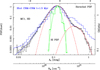 |
Fig. 6 PDFs from a SILCC-Zoom simulation together with the observed Draco PDF. The blue line shows the total hydrogen N-PDF at the 1.5 Myr timestep of the HD MC1 simulation (Seifried et al. 2017), which includes the CNM and UNM; see Sect. 1. The black line is the observed N-PDF of Draco, the green line the H I-PDF of Draco obtained from EBHIS, and the dashed red curves are the log-normal fits of the observed N-PDF. See also Fig. B.1. |
4 Conclusions
Summarizing our results, we have a scenario in which high-density (up to 103 cm−3), cold (T ~ 10-20 K), and small molecular gas clumps with a low filling factor (Miville-Deschênes et al. 2017) are embedded in a more diffuse atomic phase (n < 50 cm−3, T ~ 100 K). Cooling via dust and atomic FIR lines, mainly the [Cii] 158 μm line and the [Ci] 609 μm line (Glover et al. 2015), would also explain the nearly bimodal gas distribution, i.e. the atomic and molecular CNM phase that also causes the double log-normal N-PDF. The expected [C ii] and [Ci] intensities, however, are estimated to be extremely low (Clark et al. 2019). On the other hand, if shocks are involved, the clump surfaces would be significantly heated and could then be traced in [C ii], for example. This is indeed the case, as shown by Schneider et al. (2024), who report the detection of the [C ii] line in Draco at the position of dense clumps.
The dynamical scenario for H2 formation (e.g. Ballesteros-Paredes et al. 1999; Hartmann et al. 2001; Vázquez-Semadeni et al. 2006; Heitsch et al. 2006; Banerjee et al. 2009; Audit & Hennebelle 2010; Clark et al. 2012; Valdivia et al. 2016; Seifried et al. 2017; Colman et al. 2025) depicts a picture in which warm, trans-sonically turbulent H i flows are converging and the compression of H i gas causes the gas to cool via thermal instability to form high-density H2 (e.g. Walder & Folini 1998; Audit & Hennebelle 2005; Klessen & Hennebelle 2010). in Draco, the scenario may be somewhat different because the Draco iVC has a significant velocity of around −23 km s−1 and falls through the WNM onto the Galactic disc. Regardless of whether the iVC has its origin in extragalactic gas infall or from a Galactic fountain process, WNM gas is compressed and cooling then leads to the nearly instantaneous formation of atomic CNM and H2 clumps. in the cold, supersonic H2 phase, a 2-to-1 ratio between the energy in solenoidal and compressive modes is established, so the estimated b value for this mixed case is ~0.3-0.5 (Federrath et al. 2010), which is consistent with our value of b.
Draco can thus not be considered a typical example of colliding H i flows, in particular because the existing ‘flows’, the HVC and iVC, have no velocity link and are well separated (Fig. 1). Moreover, Draco is probably a special type of cloud in which the density structure and chemistry are influenced by shocks that naturally occur during the passage of the iVC through the WNM. A similar scenario was suggested by Bieging & Kong (2024) based on simulations of Saury et al. (2014), in which supersonic turbulence is created as the infalling iVC encounters the WNM layer in the Galactic plane, leading to a rapid formation of CO.
We propose that the shock compression leads to a large distribution of small H2 clumps embedded in the atomic phase. We note that the FiR emission in high-density regions in Draco is unusually high, compared to other iVCs, which could be an indication of shock heating. This was first seen in IRAS (Infrared Astronomical Satellite) 12 and 25 μm maps (Odenwald & Rickard 1987) and then in Herschel flux maps (Miville-Deschênes et al. 2017; Schneider et al. 2024). Again, Schneider et al. (2024) demonstrate that shock excitation can be responsible for the high FIR intensities.
We presume that Draco is seen in an early evolutionary phase and that it will continue to grow in mass via accretion from the surrounding atomic gas that becomes molecular at the stagnation point above a certain extinction value, as suggested in the numerical simulations by Heitsch et al. (2006) and Clark et al. (2012).
Acknowledgements
N.S. and E.K. acknowledge support from the FEEDBACK plus project that was supported by the BMWI via DLR, Projekt Number 50 OR 2217. This work was supported by the Collaborative Research Center 1601 (SFB 1601 sub-projects A6, B1, B2, B4) funded by the Deutsche Forschungsgemeinschaft (DFG, German Research Foundation) - 500700252. S.D. acknowledges support from the International Max Planck Research School (IMPRS) for Astronomy and Astrophysics at the Universities of Bonn and Cologne. A.K. was supported in part by the NASA Grant 80NSSC22K0724.
Appendix A The Herschel column density map
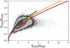 |
Fig. A.1 Colour-colour plot of the Herschel 250/350 μm vs 250/500 μm ratios. Blue, green, yellow, and red curves are theoretical colour-colour curves for a dust emissivity index β = 0, 1, 2, and 3, respectively. Contours mark the 68%, 95%, and 99% confidence levels. |
The Herschel hydrogen column density map was derived following the methodology described in Schneider et al. (2022). This approach involves a pixel-by-pixel grey-body fit to the spectral energy distribution (SED), utilizing the Herschel flux maps at 160, 250, 350, and 500 μm, all convolved to a common angular resolution of 36″ . This method is widely adopted within the astrophysical community and has been extensively referenced (André et al. 2010; Russeil et al. 2013; Lombardi et al. 2014; Schneider et al. 2015c; Stutz & Kainulainen 2015; Pokhrel et al. 2020; Spilker et al. 2021; Schneider et al. 2022). All maps were subjected to absolute flux calibration. The zeroPointCorrection task in HIPE was employed for SPIRE and IRAS maps and PACS data. SPIRE maps were calibrated for extended emission. The SED fitting procedure assumed a fixed specific dust opacity per unit mass (dust+gas) characterized by the power law κν = 0.1 (ν/1000 GHz)β cm2/g, with β = 2, while leaving the dust temperature and column density as free parameters (see Hill et al. 2011; Russeil et al. 2013; Roy et al. 2013, for details). For Draco, calibration uncertainties of 10% for SPIRE and 20% for PACS were applied to weight data points at each wavelength. In Schneider et al. (2022), an alternative weighting using full noise maps was tested but was found not to have an impact due to the high signal-to-noise ratio of the Herschel data. Draco is expected to exhibit diffuse cloud conditions with minimal ice accretion or dust coagulation. Based on Planck observations, Juvela et al. (2015) derived a dust opacity value of κν = 2.16 × 10⁻²⁵ cm−2/H for such regions, consistent with standard interstellar reddening, which we adopted for Draco.
To assess potential contributions from the cosmic infrared background and unresolved extragalactic point sources, we constructed a colour-colour diagram using the S250/S350 and S250/S500 ratios (Fig. A.1). The pixel distribution closely resembles typical Galactic values, suggesting minimal contamination from extragalactic sources or cosmic infrared background anisotropies. Potential contributions appear as outliers, located within S250/S350 ratios of 1-1.5 and S250/S500 ratios of 6-12, with an estimated contribution of less than a few percent. These results confirm that a dust emissivity index of β = 2 provides an excellent fit to the data. Opacity, dust temperature, and β maps of Draco, based on Planck data, were previously presented in Irfan et al. (2019, see their Fig. 15), showing significant variation depending on the method employed (e.g. premise, GNILC, or 2013). Bieging & Kong (2024) cite a study of Singh & Martin (2022) who used a SED fitting method with variable β and obtained a total hydrogen column density map that is a factor of 3 lower than what is obtained by Schneider et al. (2022) and Bieging & Kong (2024). Summarizing, while a detailed comparison of methods for deriving column density maps from Planck and Herschel is an important topic, it lies beyond the scope of this study. Using the simple conversion of the 250 μm Herschel flux map into a total hydrogen column density with N(H) = 2.49× 10²⁰ I(250) [MJy sr−1] H atoms/cm2 (Miville-Deschênes et al. 2017) results in a column density map that is typically 30% to 50% higher than what we obtained with the SED fit. One reason could be that because the calibration of the dust opacity is performed at long wavelengths with Planck data, typically at 353 GHz, a change of the wavelength exponent β affects the opacity and thus column density estimation at smaller wavelength, in this case at 250 μm. We used β=2, in contrast to the β of around 1.6 used in Miville-Deschenes et al. Hence, the dust model assumed here has a higher opacity at 250 μm, thus translating into a somewhat lower column density on our map. We note also that relying solely on one wavelength is inherently less reliable compared to a full SED fit across multiple wavelengths. A detailed discussion of the uncertainties related to the different methods how to obtain a column density map in Draco is found in Bieging & Kong (2024).
Appendix B N-PDF
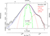 |
Fig. B.1 N-PDF of Draco from Schneider et al. (2022). The black histogram indicates the N-PDF obtained from Herschel data and the blue line its analytic description. The dashed red line gives the fit of two lognormal PDFs and takes into consideration the noise contribution that leads to a nearly linear behaviour at low column densities (Ossenkopf-Okada et al. 2016). The green histogram displays the NHI-PDF of the HI data, and the continuous line a single log-normal fit. The fitted peak positions of the PDFs and the widths (σ in units of η=ln(N/〈N〉)) are given in the panel. Error bars are based on the method presented in Jaupart & Chabrier (2022). The left y-axis gives the probability value for the Herschel map, and the right y-axis for the H I map. |
Figure B.1 shows the N-PDF of Draco obtained from Herschel and Hi EBHIS data and presented in Schneider et al. (2024). The shapes of the PDFs are discussed in detail in Schneider et al. (2022). We note that the width of the H i PDF will be systematically underestimated because of the low angular resolution of 10′ of the Hi map (Schneider et al. 2015c; Ossenkopf-Okada et al. 2016). The location of the peak of the PDF, however, is unaffected by the spatial resolution (see the appendix in Schneider et al. (2015c). We updated the PDF determination by using the proper ergodic theory developed by Jaupart & Chabrier (2022) for the estimate of the uncertainties in a finite map. It compares the size of correlated regions in the individual column density bins to the total number of samples in that bin. We used two different approaches to practically measure this size. In an isotropic approximation, we fitted the correlation length, lcorr, and obtained the size as  . In a discretized approach, we counted the pixels in the 2D auto-correlation function that fall above a level of 1/e. In general, the results of the two approaches agree well, within 10-20 %. To be conservative, we always used the larger of the two values to compute the error bars here. It turns out that for AV values between 0.025 and 0.5, the error bars hardly differ from those shown in Schneider et al. (2022). The uncertainty becomes somewhat larger for AV > 0.7, slightly modifying our fit result but not changing any of the conclusions drawn in Schneider et al. (2022).
References
- André, P., Men’shchikov, A., Bontemps, S., et al. 2010, A&A, 518, L102 [NASA ADS] [CrossRef] [EDP Sciences] [Google Scholar]
- Audit, E., & Hennebelle, P. 2005, A&A, 433, 1 [CrossRef] [EDP Sciences] [Google Scholar]
- Audit, E., & Hennebelle, P. 2010, A&A, 511, A76 [NASA ADS] [CrossRef] [EDP Sciences] [Google Scholar]
- Ballesteros-Paredes, J., Hartmann, L., & Vázquez-Semadeni, E. 1999, ApJ, 527, 285 [NASA ADS] [CrossRef] [Google Scholar]
- Ballesteros-Paredes, J., Vázquez-Semadeni, E., Gazol, A., et al. 2011, MNRAS, 416, 1436 [NASA ADS] [CrossRef] [Google Scholar]
- Banerjee, R., Vázquez-Semadeni, E., Hennebelle, P., & Klessen, R. S. 2009, MNRAS, 398, 1082 [NASA ADS] [CrossRef] [Google Scholar]
- Bellomi, E., Godard, B., Hennebelle, P., et al. 2020, A&A, 643, A36 [NASA ADS] [CrossRef] [EDP Sciences] [Google Scholar]
- Benedettini, M., Schisano, E., Pezzuto, S., et al. 2015, MNRAS, 453, 2036 [NASA ADS] [CrossRef] [Google Scholar]
- Bialy, S., & Sternberg, A. 2019, ApJ, 881, 160 [NASA ADS] [CrossRef] [Google Scholar]
- Bialy, S., Burkhart, B., & Sternberg, A. 2017, ApJ, 843, 92 [NASA ADS] [CrossRef] [Google Scholar]
- Bieging, J. H., & Kong, S. 2024, MNRAS, 531, 4138 [Google Scholar]
- Blagrave, K., Martin, P. G., Joncas, G., et al. 2017, ApJ, 834, 126 [Google Scholar]
- Bohlin, R. C., Savage, B. D., & Drake, J. F. 1978, ApJ, 224, 132 [Google Scholar]
- Burkhart, B., & Lazarian, A. 2012, ApJ, 755, L19 [NASA ADS] [CrossRef] [Google Scholar]
- Clark, P. C., Glover, S. C. O., Klessen, R. S., & Bonnell, I. A. 2012, MNRAS, 424, 2599 [CrossRef] [Google Scholar]
- Clark, P. C., Glover, S. C. O., Ragan, S. E., & Duarte-Cabral, A. 2019, MNRAS, 486, 4622 [Google Scholar]
- Colman, T., Hennebelle, P., Brucy, N., et al. 2025, arXiv e-prints, [arXiv:2503.03305] [Google Scholar]
- Desert, F. X., Bazell, D., & Boulanger, F. 1988, ApJ, 334, 815 [NASA ADS] [CrossRef] [Google Scholar]
- Dobbs, C. L. 2008, MNRAS, 391, 844 [NASA ADS] [CrossRef] [Google Scholar]
- Draine, B. T. 1978, ApJS, 36, 595 [Google Scholar]
- Ebagezio, S., Seifried, D., Walch, S., et al. 2023, MNRAS, 525, 5631 [NASA ADS] [CrossRef] [Google Scholar]
- Federrath, C., Klessen, R. S., & Schmidt, W. 2008, ApJ, 688, L79 [NASA ADS] [CrossRef] [Google Scholar]
- Federrath, C., Roman-Duval, J., Klessen, R. S., Schmidt, W., & Mac Low, M. M. 2010, A&A, 512, A81 [NASA ADS] [CrossRef] [EDP Sciences] [Google Scholar]
- Field, G. B., Goldsmith, D. W., & Habing, H. J. 1969, ApJ, 155, L149 [NASA ADS] [CrossRef] [Google Scholar]
- Gazol, A., & Kim, J. 2013, ApJ, 765, 49 [Google Scholar]
- Gillmon, K., & Shull, J. M. 2006, ApJ, 636, 908 [Google Scholar]
- Gillmon, K., Shull, J. M., Tumlinson, J., & Danforth, C. 2006, ApJ, 636, 891 [NASA ADS] [CrossRef] [Google Scholar]
- Girichidis, P., Konstandin, L., Whitworth, A. P., & Klessen, R. S. 2014, ApJ, 781, 91 [CrossRef] [Google Scholar]
- Girichidis, P., Walch, S., Naab, T., et al. 2016, MNRAS, 456, 3432 [NASA ADS] [CrossRef] [Google Scholar]
- Gladders, M. D., Clarke, T. E., Burns, C. R., et al. 1998, ApJ, 507, L161 [CrossRef] [Google Scholar]
- Glover, S. C. O. & Mac Low, M.-M. 2007, ApJ, 659, 1317 [NASA ADS] [CrossRef] [Google Scholar]
- Glover, S. C. O., & Clark, P. C. 2012, MNRAS, 421, 116 [NASA ADS] [Google Scholar]
- Glover, S. C. O., Federrath, C., Mac Low, M. M., & Klessen, R. S. 2010, MNRAS, 404, 2 [Google Scholar]
- Glover, S. C. O., Clark, P. C., Micic, M., & Molina, F. 2015, MNRAS, 448, 1607 [NASA ADS] [CrossRef] [Google Scholar]
- Godard, B., Falgarone, E., & Pineau des Forêts, G. 2014, A&A, 570, A27 [NASA ADS] [CrossRef] [EDP Sciences] [Google Scholar]
- Gry, C., Boulanger, F., Nehmé, C., et al. 2002, A&A, 391, 675 [NASA ADS] [CrossRef] [EDP Sciences] [Google Scholar]
- Habing, H. J. 1968, Bull. Astron. Inst. Netherlands, 19, 421 [Google Scholar]
- Hartmann, L., Ballesteros-Paredes, J., & Bergin, E. A. 2001, ApJ, 562, 852 [NASA ADS] [CrossRef] [Google Scholar]
- Heiles, C., & Habing, H. J. 1974, A&AS, 14, 1 [NASA ADS] [Google Scholar]
- Heiles, C., & Troland, T. H. 2003, ApJ, 586, 1067 [NASA ADS] [CrossRef] [Google Scholar]
- Heitsch, F., Slyz, A. D., Devriendt, J. E. G., Hartmann, L. W., & Burkert, A. 2006, ApJ, 648, 1052 [CrossRef] [MathSciNet] [Google Scholar]
- Hennebelle, P., & Audit, E. 2007, A&A, 465, 431 [NASA ADS] [CrossRef] [EDP Sciences] [Google Scholar]
- Hennebelle, P., Banerjee, R., Vázquez-Semadeni, E., Klessen, R. S., & Audit, E. 2008, A&A, 486, L43 [NASA ADS] [CrossRef] [EDP Sciences] [Google Scholar]
- Herbstmeier, U., Heithausen, A., & Mebold, U. 1993, A&A, 272, 514 [NASA ADS] [Google Scholar]
- Hill, T., Motte, F., Didelon, P., et al. 2011, A&A, 533, A94 [NASA ADS] [CrossRef] [EDP Sciences] [Google Scholar]
- Hollenbach, D. J., Takahashi, T., & Tielens, A. G. G. M. 1991, ApJ, 377, 192 [NASA ADS] [CrossRef] [Google Scholar]
- Imara, N., & Burkhart, B. 2016, ApJ, 829, 102 [CrossRef] [Google Scholar]
- Irfan, M. O., Bobin, J., Miville-Deschênes, M.-A., & Grenier, I. 2019, A&A, 623, A21 [NASA ADS] [CrossRef] [EDP Sciences] [Google Scholar]
- Jaupart, E., & Chabrier, G. 2022, A&A, 663, A113 [NASA ADS] [CrossRef] [EDP Sciences] [Google Scholar]
- Jura, M. 1974, ApJ, 191, 375 [NASA ADS] [CrossRef] [Google Scholar]
- Juvela, M., Ristorcelli, I., Marshall, D. J., et al. 2015, A&A, 584, A93 [NASA ADS] [CrossRef] [EDP Sciences] [Google Scholar]
- Kainulainen, J., Beuther, H., Henning, T., & Plume, R. 2009, A&A, 508, L35 [NASA ADS] [CrossRef] [EDP Sciences] [Google Scholar]
- Kalberla, P. M. W. 2025, A&A, 694, L11 [NASA ADS] [CrossRef] [EDP Sciences] [Google Scholar]
- Kalberla, P. W. M., Herbstmeier, U., & Mebold, U. 1984, in NASA Conference Publication, 2345, 243 [Google Scholar]
- Kerp, J., Lenz, D., & Röhser, T. 2016, A&A, 589, A123 [NASA ADS] [CrossRef] [EDP Sciences] [Google Scholar]
- Klessen, R. S., & Glover, S. C. O. 2016, Saas-Fee Adv. Course, 43, 85 [NASA ADS] [CrossRef] [Google Scholar]
- Klessen, R. S., & Hennebelle, P. 2010, A&A, 520, A17 [NASA ADS] [CrossRef] [Google Scholar]
- Klessen, R. S., Heitsch, F., & Mac Low, M.-M. 2000, ApJ, 535, 887 [NASA ADS] [CrossRef] [Google Scholar]
- Koyama, H., & Inutsuka, S.-I. 2000, ApJ, 532, 980 [Google Scholar]
- Kritsuk, A. G., & Norman, M. L. 2004, ApJ, 601, L55 [Google Scholar]
- Kritsuk, A. G., Norman, M. L., Padoan, P., & Wagner, R. 2007, ApJ, 665, 416 [NASA ADS] [CrossRef] [Google Scholar]
- Kritsuk, A. G., Norman, M. L., & Wagner, R. 2011, ApJ, 727, L20 [NASA ADS] [CrossRef] [Google Scholar]
- Kritsuk, A. G., Ustyugov, S. D., & Norman, M. L. 2017, New J. Phys., 19, 065003 [Google Scholar]
- Krumholz, M. R., McKee, C. F., & Tumlinson, J. 2008, ApJ, 689, 865 [NASA ADS] [CrossRef] [Google Scholar]
- Lagache, G., Abergel, A., Boulanger, F., & Puget, J. L. 1998, A&A, 333, 709 [Google Scholar]
- Lee, H. H., Herbst, E., Pineau des Forets, G., Roueff, E., & Le Bourlot, J. 1996, A&A, 311, 690 [Google Scholar]
- Lenz, D., Kerp, J., Flöer, L., et al. 2015, A&A, 573, A83 [NASA ADS] [CrossRef] [EDP Sciences] [Google Scholar]
- Li, Y., Klessen, R. S., & Mac Low, M.-M. 2003, ApJ, 592, 975 [Google Scholar]
- Lombardi, M., Bouy, H., Alves, J., & Lada, C. J. 2014, A&A, 566, A45 [NASA ADS] [CrossRef] [EDP Sciences] [Google Scholar]
- Mac Low, M.-M., & Klessen, R. S. 2004, Rev. Mod. Phys., 76, 125 [Google Scholar]
- Mac Low, M.-M., & Glover, S. C. O. 2012, ApJ, 746, 135 [NASA ADS] [CrossRef] [Google Scholar]
- Marchal, A., Miville-Deschênes, M.-A., Orieux, F., et al. 2019, A&A, 626, A101 [NASA ADS] [CrossRef] [EDP Sciences] [Google Scholar]
- Mebold, U., Cernicharo, J., Velden, L., et al. 1985, A&A, 151, 427 [Google Scholar]
- Micic, M., Glover, S. C. O., Federrath, C., & Klessen, R. S. 2012, MNRAS, 421, 2531 [NASA ADS] [CrossRef] [Google Scholar]
- Miville-Deschênes, M. A., Salomé, Q., Martin, P. G., et al. 2017, A&A, 599, A109 [NASA ADS] [CrossRef] [EDP Sciences] [Google Scholar]
- Molina, F. Z., Glover, S. C. O., Federrath, C., & Klessen, R. S. 2012, MNRAS, 423, 2680 [NASA ADS] [CrossRef] [Google Scholar]
- Moritz, P., Wennmacher, A., Herbstmeier, U., et al. 1998, A&A, 336, 682 [Google Scholar]
- Murray, C. E., Stanimirovic, S., Goss, W. M., et al. 2018, ApJS, 238, 14 [NASA ADS] [CrossRef] [Google Scholar]
- Nelson, R. P., & Langer, W. D. 1997, ApJ, 482, 796 [NASA ADS] [CrossRef] [Google Scholar]
- Odenwald, S. F., & Rickard, L. J. 1987, ApJ, 318, 702 [Google Scholar]
- Ossenkopf-Okada, V., Csengeri, T., Schneider, N., Federrath, C., & Klessen, R. S. 2016, A&A, 590, A104 [NASA ADS] [CrossRef] [EDP Sciences] [Google Scholar]
- Padoan, P., Jones, B. J. T., & Nordlund, A. P. 1997, ApJ, 474, 730 [NASA ADS] [CrossRef] [Google Scholar]
- Park, G., Lee, M.-Y., Bialy, S., et al. 2023, ApJ, 955, 145 [Google Scholar]
- Passot, T., & Vázquez-Semadeni, E. 1998, Phys. Rev. E, 58, 4501 [Google Scholar]
- Planck Collaboration XXIV. 2011, A&A, 536, A24 [NASA ADS] [CrossRef] [EDP Sciences] [Google Scholar]
- Pokhrel, R., Gutermuth, R. A., Betti, S. K., et al. 2020, ApJ, 896, 60 [NASA ADS] [CrossRef] [Google Scholar]
- Pound, M. W., & Wolfire, M. G. 2023, AJ, 165, 25 [NASA ADS] [CrossRef] [Google Scholar]
- Putman, M. E., Peek, J. E. G., & Joung, M. R. 2012, ARA&A, 50, 491 [Google Scholar]
- Reach, W. T., Koo, B.-C., & Heiles, C. 1994, ApJ, 429, 672 [NASA ADS] [CrossRef] [Google Scholar]
- Rohlfs, R., Herbstmeier, U., Mebold, U., & Winnberg, A. 1989, A&A, 211, 402 [NASA ADS] [Google Scholar]
- Röhser, T., Kerp, J., Winkel, B., Boulanger, F., & Lagache, G. 2014, A&A, 564, A71 [NASA ADS] [CrossRef] [EDP Sciences] [Google Scholar]
- Röhser, T., Kerp, J., Ben Bekhti, N., & Winkel, B. 2016a, A&A, 592, A142 [NASA ADS] [CrossRef] [EDP Sciences] [Google Scholar]
- Röhser, T., Kerp, J., Lenz, D., & Winkel, B. 2016b, A&A, 596, A94 [NASA ADS] [CrossRef] [EDP Sciences] [Google Scholar]
- Röllig, M., & Ossenkopf-Okada, V. 2022, A&A, 664, A67 [NASA ADS] [CrossRef] [EDP Sciences] [Google Scholar]
- Röllig, M., Ossenkopf, V., Jeyakumar, S., Stutzki, J., & Sternberg, A. 2006, A&A, 451, 917 [Google Scholar]
- Röllig, M., Abel, N. P., Bell, T., et al. 2007, A&A, 467, 187 [Google Scholar]
- Roy, A., Martin, P. G., Polychroni, D., et al. 2013, ApJ, 763, 55 [Google Scholar]
- Russeil, D., Schneider, N., Anderson, L. D., et al. 2013, A&A, 554, A42 [NASA ADS] [CrossRef] [EDP Sciences] [Google Scholar]
- Saury, E., Miville-Deschênes, M. A., Hennebelle, P., Audit, E., & Schmidt, W. 2014, A&A, 567, A16 [NASA ADS] [CrossRef] [EDP Sciences] [Google Scholar]
- Schneider, N., André, P., Könyves, V., et al. 2013, ApJ, 766, L17 [NASA ADS] [CrossRef] [Google Scholar]
- Schneider, N., Bontemps, S., Girichidis, P., et al. 2015a, MNRAS, 453, L41 [CrossRef] [Google Scholar]
- Schneider, N., Csengeri, T., Klessen, R. S., et al. 2015b, A&A, 578, A29 [NASA ADS] [CrossRef] [EDP Sciences] [Google Scholar]
- Schneider, N., Ossenkopf, V., Csengeri, T., et al. 2015c, A&A, 575, A79 [CrossRef] [EDP Sciences] [Google Scholar]
- Schneider, N., Ossenkopf-Okada, V., Clarke, S., et al. 2022, A&A, 666, A165 [NASA ADS] [CrossRef] [EDP Sciences] [Google Scholar]
- Schneider, N., Bonne, L., Bontemps, S., et al. 2023, Nat. Astron., 7, 546 [NASA ADS] [CrossRef] [Google Scholar]
- Schneider, N., Ossenkopf-Okada, V., Keilmann, E., et al. 2024, A&A, 686, A109 [NASA ADS] [CrossRef] [EDP Sciences] [Google Scholar]
- Seifried, D., Schmidt, W., & Niemeyer, J. C. 2011, A&A, 526, A14 [NASA ADS] [CrossRef] [EDP Sciences] [Google Scholar]
- Seifried, D., Walch, S., Girichidis, P., et al. 2017, MNRAS, 472, 4797 [NASA ADS] [CrossRef] [Google Scholar]
- Seifried, D., Beuther, H., Walch, S., et al. 2022, MNRAS, 512, 4765 [NASA ADS] [CrossRef] [Google Scholar]
- Singh, A., & Martin, P. G. 2022, ApJ, 941, 135 [CrossRef] [Google Scholar]
- Spilker, A., Kainulainen, J., & Orkisz, J. 2021, A&A, 653, A63 [NASA ADS] [CrossRef] [EDP Sciences] [Google Scholar]
- Sternberg, A., & Dalgarno, A. 1989, ApJ, 338, 197 [Google Scholar]
- Sternberg, A., Le Petit, F., Roueff, E., & Le Bourlot, J. 2014, ApJ, 790, 10 [CrossRef] [Google Scholar]
- Stutz, A. M., & Kainulainen, J. 2015, A&A, 577, L6 [NASA ADS] [CrossRef] [EDP Sciences] [Google Scholar]
- Tielens, A. G. G. M., & Hollenbach, D. 1985, ApJ, 291, 722 [Google Scholar]
- Tremblin, P., Schneider, N., Minier, V., et al. 2014, A&A, 564, A106 [NASA ADS] [CrossRef] [EDP Sciences] [Google Scholar]
- Valdivia, V., Hennebelle, P., Gérin, M., & Lesaffre, P. 2016, A&A, 587, A76 [NASA ADS] [CrossRef] [EDP Sciences] [Google Scholar]
- van Dishoeck, E. F., & Black, J. H. 1988, ApJ, 334, 771 [Google Scholar]
- van Dishoeck, E. F., & Black, J. H. 1986, ApJS, 62, 109 [Google Scholar]
- Vazquez-Semadeni, E. 1994, ApJ, 423, 681 [Google Scholar]
- Vázquez-Semadeni, E., Ryu, D., Passot, T., González, R. F., & Gazol, A. 2006, ApJ, 643, 245 [Google Scholar]
- Visser, R., van Dishoeck, E. F., & Black, J. H. 2009, A&A, 503, 323 [NASA ADS] [CrossRef] [EDP Sciences] [Google Scholar]
- Walch, S., Girichidis, P., Naab, T., et al. 2015, MNRAS, 454, 238 [Google Scholar]
- Walder, R., & Folini, D. 1998, A&A, 330, L21 [NASA ADS] [Google Scholar]
- Winkel, B., Kerp, J., Flöer, L., et al. 2016, A&A, 585, A41 [NASA ADS] [CrossRef] [EDP Sciences] [Google Scholar]
- Wolfire, M. G., Hollenbach, D., McKee, C. F., Tielens, A. G. G. M., & Bakes, E. L. O. 1995, ApJ, 443, 152 [Google Scholar]
- Wolfire, M. G., McKee, C. F., Hollenbach, D., & Tielens, A. G. G. M. 2003, ApJ, 587, 278 [Google Scholar]
- Wolfire, M. G., Hollenbach, D., & McKee, C. F. 2010, ApJ, 716, 1191 [Google Scholar]
- Zucker, C., Speagle, J. S., Schlafly, E. F., et al. 2020, A&A, 633, A51 [NASA ADS] [CrossRef] [EDP Sciences] [Google Scholar]
The FUV field is expressed in units of Habing Go (Habing 1968) or Draine χ (Draine 1978), where χ = 1.71 Go.
We used the conversion NH/AV = 1.87 × 1021 cm−2 mag−1 (Bohlin et al. 1978) to relate the total hydrogen column density to the visual extinction.
The distance to the iVC was initially estimated to be between 463 and 618 pc (with an uncertainty of −200 pc) by Gladders et al. (1998), using sodium doublet absorption measurements. Here, we adopt the more recent distance of 481 ± 50 pc, determined by Zucker et al. (2020) based on Gaia DR2 parallax measurements.
SImulating the LifeCycle of molecular Clouds; http://www.astro.uni-koeln.de/-silcc.
There is some uncertainty concerning the molecular fraction in Draco. Schneider et al. (2022) determined as a global average that −10% of the total gas in Draco is molecular, Moritz et al. (1998) obtained spatially varying values between 0 and 50%, and Bieging & Kong (2024) show the detailed distribution of molecular fraction over the dense filaments, with 90% only in the highest column density areas.
All Figures
|
Fig. 1 Draco cloud in HI. Left: channel maps of HI brightness temperature in K from EBHIS at 10′ angular resolution in steps of 4 km s−1. The central velocity is given in the lower-left corner, and the individual velocity components of Draco (high, intermediate, and local) are indicated. Right: zoom into the velocity range of the IVC between −12 and −28 km s−1 using the DRAO with the Synthesis Telescope H I data at 1′ angular resolution (Blagrave et al. 2017) in steps of 0.82 km s−1. |
| In the text | |
|
Fig. 2 Draco total hydrogen column density map (N(H)) and CO 2→1 contours. The Herschel N(H) map (Schneider et al. 2022, 2024) has an angular resolution of 36″. The 12CO 2→1 data have a resolution of 38″ and stem from Bieging & Kong (2024). The contours are 2, 7, and 12 K km s−1. |
| In the text | |
|
Fig. 3 H I-to-H2 transitional AV as a function of UV field and the clump-averaged density 〈n〉, determined from the KOSMA-tau PDR model. The colour wedge gives the value of AV, and the white line indicates our observed transitional AV of 0.33. |
| In the text | |
|
Fig. 4 Parameter space for the Mach number and b parameter. The diagram displays the variation in M and b as a function of the H I line width and temperature for the HD case (dotted line) and the magnetic case (straight line). |
| In the text | |
|
Fig. 5 PDF from a MHD simulation (magnetic field strength B = 3μG) of forced multi-phase turbulence (Kritsuk & Norman 2004; Kritsuk et al. 2017) in a 200 pc box with a mean HI density of 5 cm−3 and a velocity dispersion of 16 km s−1. The WNM is represented by the green line, the CNM (atomic and molecular) by the blue line. |
| In the text | |
|
Fig. 6 PDFs from a SILCC-Zoom simulation together with the observed Draco PDF. The blue line shows the total hydrogen N-PDF at the 1.5 Myr timestep of the HD MC1 simulation (Seifried et al. 2017), which includes the CNM and UNM; see Sect. 1. The black line is the observed N-PDF of Draco, the green line the H I-PDF of Draco obtained from EBHIS, and the dashed red curves are the log-normal fits of the observed N-PDF. See also Fig. B.1. |
| In the text | |
|
Fig. A.1 Colour-colour plot of the Herschel 250/350 μm vs 250/500 μm ratios. Blue, green, yellow, and red curves are theoretical colour-colour curves for a dust emissivity index β = 0, 1, 2, and 3, respectively. Contours mark the 68%, 95%, and 99% confidence levels. |
| In the text | |
|
Fig. B.1 N-PDF of Draco from Schneider et al. (2022). The black histogram indicates the N-PDF obtained from Herschel data and the blue line its analytic description. The dashed red line gives the fit of two lognormal PDFs and takes into consideration the noise contribution that leads to a nearly linear behaviour at low column densities (Ossenkopf-Okada et al. 2016). The green histogram displays the NHI-PDF of the HI data, and the continuous line a single log-normal fit. The fitted peak positions of the PDFs and the widths (σ in units of η=ln(N/〈N〉)) are given in the panel. Error bars are based on the method presented in Jaupart & Chabrier (2022). The left y-axis gives the probability value for the Herschel map, and the right y-axis for the H I map. |
| In the text | |
Current usage metrics show cumulative count of Article Views (full-text article views including HTML views, PDF and ePub downloads, according to the available data) and Abstracts Views on Vision4Press platform.
Data correspond to usage on the plateform after 2015. The current usage metrics is available 48-96 hours after online publication and is updated daily on week days.
Initial download of the metrics may take a while.