| Issue |
A&A
Volume 699, July 2025
|
|
|---|---|---|
| Article Number | A20 | |
| Number of page(s) | 11 | |
| Section | Stellar structure and evolution | |
| DOI | https://doi.org/10.1051/0004-6361/202555264 | |
| Published online | 25 June 2025 | |
Digging deeper for RR Lyrae stars with low modulation amplitudes
Konkoly Observatory, Research Center for Astronomy and Earth Sciences of HUN-REN, Budapest, 1121 Konkoly Thege ut. 15-17, Hungary
⋆ Corresponding author: This email address is being protected from spambots. You need JavaScript enabled to view it.
Received:
23
April
2025
Accepted:
18
May
2025
Abstract
With the goal of searching for very low modulation amplitudes among fundamental mode RR Lyrae stars and assessing their incidence rate, we performed a survey of 36 stars observed by the Kepler satellite over the entire four-year period of its mission. The search was conducted by a task-oriented code, designed to find low-amplitude signals in the presence of high-amplitude components and instrumental systematics. We found six new modulated stars and negated one earlier claimed star, thereby increasing the number of known Blazhko stars from 18 to 24 and yielding an observed occurrence rate of 67% for the Kepler field. Five of the new stars have the lowest modulation amplitudes found so far, with ∼250 ppm Fourier side-lobe amplitudes near the fundamental mode frequency. Because of the small sample size in the Kepler field, we extended the survey to 12 campaign fields observed by K2, the two-wheeled mission of Kepler. From the 1061 stars, we identified 514 Blazhko stars. After correcting for the short duration of the time spent on each field and for the noise dependence of the detections, we arrived at an underlying occurrence rate of ∼75% – likely a lower limit for the true rate of Blazhko stars in the K2 fields.
Key words: surveys / stars: variables: RR Lyrae
© The Authors 2025
 Open Access article, published by EDP Sciences, under the terms of the Creative Commons Attribution License (https://creativecommons.org/licenses/by/4.0), which permits unrestricted use, distribution, and reproduction in any medium, provided the original work is properly cited.
This article is published in open access under the Subscribe to Open model. This email address is being protected from spambots. You need JavaScript enabled to view it. to support open access publication.
1. Introduction
RR Lyrae stars are unique objects among the large-amplitude variables. At least half of the fundamental mode (RRab) stars show periodic light curve modulation, commonly known as the Blazhko phenomenon (see Blazhko 1907, Shapley 1916, and Szeidl & Kolláth 2000 for some historical background). The modulation amplitudes vary in a wide range from object to object, occasionally reaching the size of the amplitude of the pulsation. A large number of observational studies have been devoted to these stars over the past hundred years, without leading to any clue to the root cause of this mesmerizing physical phenomenon.
Among the various observables that could play a role in the discovery of the basic physics behind the modulation, here we focus on the frequency of the Blazhko objects. Because measurement accuracy and data volume (especially the length of the time base) obviously play an important role in the detectability of the modulation, we used the single-field data from the nearly four-year-long Kepler mission, and that of the extended mission K21, covering various fields but with a much shorter duration of ∼80 days each. Although both of these sets are of (very) high quality, the high stellar density in the Kepler field is a serious issue, in particular, when the various quarters are to be merged for a joint analysis. Similarly, in the light of the analysis of the OGLE (Optical Gravitational Lensing Experiment) Galactic Bulge data by Prudil & Skarka (2017) and Skarka et al. (2020), the K2 data surely miss many objects with long-period modulations. In spite of these and some other drawbacks such as the low sample size for the Kepler data and the overwhelming instrumental noise for many of the stars in the K2 data, these sets obviously belong to the indispensable data domain in the present context.
Observed occurrence rates reported so far for modulated RRab stars from various stellar populations range from the ridiculously low 12% (field stars in the Large Magellanic Cloud, via the Massive Compact Halo Objects or MACHO survey – see Alcock et al. 2003) to the shockingly high ∼90% (Galactic field, from the analysis of several K2 fields by Kovacs 2018, 2021). The importance of the sample size and, in particular, of the data precision can be further illustrated by the change from the earlier estimate of 20 − 30% for Galactic field stars (Szeidl 1988) to the almost 50%, estimated later by Jurcsik et al. (2009) from a small (i.e., 30) but high-quality sample. Similarly for the Galactic Bulge, from a relatively small sample of 150 stars from the OGLE-I inventory, Moskalik & Poretti (2003) derive ∼20%, whereas from the accumulated data of ∼8000 stars by the domination of the observations made in the OGLE-IV phase, Prudil & Skarka (2017) arrives at ∼40%.
Here, focusing solely on RRab stars and following the methodology described in Sect. 2, we perform a frequency analysis for the combined data of nearly all quarters of the original Kepler mission. We also extend our earlier work on the K2 campaign fields and search for RR Lyrae stars with low modulation amplitudes. The basic question we intend to address is whether there is a real dearth of low-amplitude Blazhko stars, or whether the data are still insufficient to address this question. In other words, we ask whether all non-detections are attributable to genuine unmodulated monoperiodic fundamental-mode pulsators.
2. Method
With some important modifications, here we essentially follow the methodology used in our previous papers concerning modulated RR Lyrae stars (Kovacs 2018, 2021). The basic steps and signal constituents are depicted in Fig. 1. Below, we describe the most important features of the data handling and analysis2.
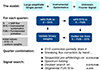 |
Fig. 1. Brief summary of the time series procedures employed in this work to search for modulated RR Lyrae stars. The prefix “w” in wFit denotes a weighted least squares fit, controlled by the outlier array, generated during the fitting cycle. Additional details can be found in Sect. 2. |
Signal component separation. The fundamental problem in discovering a shallow signal in the presence of a large signal (hereafter referred to as FUN) and instrumental systematics (hereafter referred to as SYS) is the separation of these constituents with a minimum distortion of the components, including the unknown component. The separation of the components is executed in a simple iteration loop. Because the shallow signal is unknown, we cannot include it in the iteration, except if, at each step of the iteration, a frequency analysis is performed on the residuals X-FUN-SYS, where X denotes the input signal, i.e., the raw data, usually obtained from simple aperture photometry (SAP). This, however, could be extremely expensive computationally, and, based on our earlier efforts, does not seem to be profitable in terms of the discovery of new signals. Therefore, only FUN and SYS are involved in the iteration, and, then, when the iteration is complete, the residuals X-FUN-SYS are searched for new signals.
The systematics correction vector. We employed co-trending to filter out instrumental systematics via simple weighted least squares. Co-trending is based on the assumption that systematics can be modeled by using the linear combination of non-variable stars measured simultaneously in the same field where the target is (Kovacs et al. 2005; Tamuz et al. 2005; Smith et al. 2012). The correction time series (or vectors) are built up from a properly selected set of non-variable stars. Then, this set is run through some standard dimension reduction methods (e.g., Singular Value Decomposition, or SVD – see Press et al. 1992), whereby a new set of vectors is constructed from all the vectors selected in the first step. These SVD vectors are ordered according to “essentiality”, and some fraction of them is used as SYS. For the Kepler data, we employed about 10–30, whereas for K2, we used 100 SVD vectors (constructed from ∼500 stars in each field). It is important to note that target-dependent external parameters (such as photocenter pixel positions – see Bakos et al. 2010) were not used in this work, because they could lead to considerable signal distortion and do not result in a higher signal detection rate.
Quarterly fit of FUN and SYS. For the systematics correction vectors SYS, it is clear that the fit is performed on a quarterly basis. However, when global functions (functions that are assumed to be independent of the quarters) are also included in the model, this is no longer true. In general, the signals we search for are in the ppt (parts per thousand) – sub-ppt regime. Our experimentation with the model including FUN as a global function suggests that this approach always leaves extra power very close to the fundamental mode frequency, f0, and its harmonics, making the detection of nearby faint signal components more difficult. Consequently, we opted for a quarterly based FUN fit and assumed that the very small differences among the resulting solutions for FUN reflect the remaining minor systematics that were not filtered by the previous systematics correction steps. Obviously, if the modulation has a small amplitude and long period, this method suppresses the modulation, and this particular property of the target thereby remains hidden. Nevertheless, the quarterly separate fits are in line with the way we treated the K2 time series, and the short-period Blazhko phenomena (with PBL 50 days) can still be very well studied and provide warning signs at moderately longer periods.
Outlier selection. In many cases, outliers could cause trouble if they are not treated correctly. After some experimentation with a robust fit algorithm, we opted for a “milder” approach by using a simple sigma-clipping method during the iterative phase of the systematics filtering. It is important to note that we selected the outliers from X-FUN-SYS and began with uniform weights. Once an initial outlier label array was generated, we used this array in the weighted least squares fits. With a properly chosen sigma-clipping factor (usually between 3.5 and 5-times of the standard deviation), at each iteration the weight array was updated with 0 or 1, depending on the current outlier status of the given data item.
Quarter stitching. For the Kepler data, where seasonal segments (quarters) are available, a particular issue is the combination of those segments. Because the leading cause of the different flux variations from quarter to quarter is the sneaking in and out of neighboring stars into the aperture where the raw flux is measured, we opted to use a single parameter, instead of using two proper flux-adjusting parameters (e.g., Nemec et al. 2011; Benkő et al. 2014). This parameter is constant throughout the full span of a given quarter but varies between the different quarters, and, of course, it is also target dependent. The sneaking flux correction was applied to the raw (i.e., SAP) flux as follows:
 (1)
(1)
where Xraw(i) is the i-th input (actually measured) stellar flux and Fsneak is the properly adjusted sneak flux for a given target and a given quarter. Because the systematics corrections are quarter-dependent, most of the adjustment was already done via the iterated SYS time series. Fsneak was needed to tackle the uncorrected part. The value of Fsneak was selected on a trial and error basis after an inspection of either the multi-quarter, systematics-corrected signal X-SYS, or the variation of the temporal Fourier fits (see below).
Modulation diagnostics. The basic diagnostic tool is the prewhitened Fourier spectrum3 (DFT – Discrete Fourier Transform, Deeming 1975). The lack of residual power near the fundamental mode frequency f0 and/or its harmonics disqualifies any further inquiry about a possible modulation component4.
Assuming repeating frequency patterns around f0 and its harmonics, the above spectrum can be used to compute the folded Fourier spectrum. Here, we simply added up the power (i.e., the square of the amplitudes obtained from DFT) in the ±f0/2 neighborhood of f0 and its harmonics throughout the evaluated spectrum. We used the square root of the derived power spectrum to maintain compatibility with the original DFT spectrum.
In the method of doublet search, we assume that the prewhitened time series X-FUN-SYS can be approximated by frequency doublets around f0 and its harmonics (here, we used frequencies up to the 5th harmonics). By changing the modulation frequency fmod, we fit these doublets to X-FUN-SYS, computed the RMS of the fit, and searched for the minimum value. Although an exact repeating frequency distribution does not seem to be present in all cases, this method is proven to be the most powerful diagnostic to detect very shallow modulation components barely seen in the DFT spectrum.
Lastly, following Nemec et al. (2011), in the method of segmental FUN fit, we used overlapping small segments of the full light curve X-SYS (corrected for sneaking fluxes in the multi-quarter case) to fit FUN and use the temporal Fourier amplitudes and phases (A1(t) and φ1(t), respectively) at f0. The pattern observed in these Fourier parameters is also a very powerful diagnostic tool and weighs in on the final evaluation of a given target.
Simple light curve inspection. Serving as an overall data quality assessment, all the above can be combined by inspecting the full light curve (including the raw data) and the close-ups of the upper and lower envelopes of the systematics-filtered light curves. Examples of the diagnostic diagrams are shown in Figs. 2 and 6.
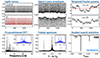 |
Fig. 2. Example of diagnostic diagrams for an RR Lyrae star from the Kepler field, used in search for modulated stars. Upper row, from left to right: Systematics-corrected (upper subpanel) and raw light curves; units on the horizontal and vertical axes are in days and relative magnitudes, respectively. Close-up of the lower and upper parts (respectively, upper and lower halves of the panel) of the filtered light curve shown in the first panel (units are the same as in the first panel). Variation (relative to the average) of the time-dependent Fourier parameters at the fundamental frequency f0. The red line indicates the linear regression to ΔA1(t). Vertical axis units: [ppt] and [rad]. Lower row, from left to right: Full DFT of the prewhitened data, with the inset zooming on the region of f0 (the horizontal axis shows f − f0). Folded spectrum, with a similar plot structure as in the previous panel. RMS values of the doublet search at various modulation frequencies. The KIC ID (also known as V1510 Cyg) is shown in the lower right corner. All vertical axes are normalized to the peak values; horizontal axes have the same units (i.e., [c/d]). See Sect. 2 for additional details. |
Annual variation test. Because the systematics correction vector SYS is composed from bright stars, they are presumably less affected by seasonal and annual variations than the RR Lyrae stars, which are on the fainter tail of the brightness distribution. As a result, co-trending is in general not able to eliminate fully long-term systematics manifesting as fake annual modulations in several RR Lyrae stars. To test whether suspicious modulations near the time scale of a year5 and its harmonics may be related to instrumental effects, we also fit a Fourier sum to the Kepler data with frequencies {j × f0 ± k/365; j, k = 1, 2, ..,5}, and check whether the suspected component is eliminated. If so, the candidate is dropped.
Target classification. We used a simple three-level classification scheme to assess the likelihood of a modulation signal6 being present in a given target. The lack of significant residual peaks near f0 and/or its harmonics leads to class 0. Peaks close to the noise level may also lead to the above classification, if other diagnostics are not strong enough for a different classification. If the residual peak is strong, it usually leads to class 2, implying a possible long-period modulation, assuming that other diagrams do not suggest otherwise (e.g., strongly corrupted data by observational and/or instrumental effects). Finally, if all diagrams are cooperative, and, in particular, the doublet search suggests the presence of a significant signal, then the object is labeled as class 1, i.e., an RR Lyrae with a Blazhko effect. Additional complications may occur during the analysis of the K2 data, when multiple data sources are available with different classifications. In this case, we assign class 1 to the star if at least one of the sources has this classification. Otherwise, the star is labeled as class 2. This scheme favors decisions made on detections even if the data sources used to make these decisions are in the minority with respect to the remaining sets analyzed for a given target.
3. Datasets
We analyzed the RRab stars from two databases: the one gathered by the Kepler satellite during its original mission by monitoring a single field over a four-year span (Borucki 2017); and the multi-field data collected by the extended mission K2 (Howell et al. 2014) along the ecliptic belt. While during the original mission the pointing was accurate, the K2 phase was overwhelmed by instrumental systematics due to the correction mechanisms applied for the lost reaction wheels. In the rest of the paper, we refer to the data gathered during the original Kepler mission as “Kepler data”. The quarters are referred to as Q##, where the hash marks refer to the two-digit quarter numbers. The campaign fields in the case of the K2 data are similarly referred to beginning with the letter “C”.
We used only long-cadence (i.e., ∼ half-hour-integrated) data from both missions. Except for Q01, all the available quarters were employed. Most of the targets we analyze from the Kepler data contain over 60 000 data points, allowing, in principle, a search for sinusoidal signals at the level of a few times 10 ppm in the RR Lyrae sample. Following the list of Plachy & Szabó (2021), a sample of 37 RRab stars have been investigated. Although Forró et al. (2022) provides an extension of this list containing an additional 20 RRab stars, after experimenting with the data, we decided not to use these stars. The stars are mostly faint and therefore not only have greater noise but also suffer from stronger systematics due to the crowded nature of the Kepler field. With these quality factors, it is nearly impossible to discover hidden low-amplitude Blazhko stars (in particular those with long modulation periods). All the data used for the analysis of the Kepler data have been downloaded from the STScI MAST site7.
The RRab list provided by Molnár et al. (2018), Plachy et al. (2019) were used to select the targets for the K2 analysis. Although there is an updated, more extensive list by Bódi et al. (2022), we decided not to use their list (and the accompanying data) in the present analysis, because the set based on the above two lists is large enough to ensure the statistical stability of the results derived from this sample. The campaign fields covered by Molnár et al. (2018) span from C00 to C13 and include 1211 RRab stars. Extended by the list of Plachy et al. (2019), we began with the set of 1301 stars. Except for C00, all the fields were used. This results in 1061 stars, considering data availability and quality.
Fortunately, there are several data sources with published raw photometry available for the K2 fields. First, the pipeline of the mission provides easy access to these data via the MAST site. Second, a number of groups made serious efforts to treat the data using various methodologies. These studies have provided different approaches to deriving better raw and systematics-filtered photometric data. We used the following sources: Petigura et al. (2015), downloaded from the NASA ExoFop site;8Vanderburg & Johnson (2014) and Luger et al. (2016, 2018), which were downloaded from corresponding MAST sites. Thereby, when the K2 data were analyzed, we had four independent raw time series to use as inputs, and hence the final classification is certainly based on a more solid ground than if only a single source were used. Nevertheless, for various reasons (individual project preference, failed target aperture, etc.) there are cases in which not all four sources were available.
4. Results: The Kepler data
Following the method described in Sect. 2, we analyzed all 37 RRab stars as listed by Plachy & Szabó (2021). We quickly detected the 19 previously claimed Blazhko stars (including V346 Lyr, earlier identified by Benkő et al. 2019), but after many repeated analyses of the full sample, we found that KIC 007021124 did not pass our detection criteria. In particular, quarter stitching had led to seasonal changes, and no other significant variations were identifiable in any of the diagnostic diagrams. An earlier classification of this object as a Blazhko star by Benkő & Szabó (2015) is based predominantly on apparent long-term phase and light curve shape variations, which, due to its long-term nature, is hard to disentangle from the seasonal variations present in many RR Lyrae stars in the Kepler data. Therefore, we labeled this star as class 2.
Turning to the 18 stars so far classified as non-Blazhko stars, we found that, except for KIC 006100702, all show residual power near f0 and its harmonics. This object is bright (Kp = 13.46), seems unaffected by long-term systematics, lacks any other secondary signal component, and therefore looks like a genuine single-mode RRab star.
Another star, KIC 003866709, turned out to be intractable by the method we used. There are repeating flip-flopping systematics from one quarter to the other that are target specific, which do not apparently share enough commonality with the co-trending set we applied. As a result, no classification was possible for this target within our scheme. Consequently, we excluded this target from the sample.
The remaining 17 stars were thoroughly scrutinized through an examination of the various features as discussed in Sect. 2 and shown in Fig. 2, exhibiting one of our strongest detections. Because the temporal Fourier analysis works on the full (systematics-corrected and stitched) light curve, it is sensitive to local amplitude and phase variations (see upper right panel). The frequency spectra (and also the doublet search; see thelower panels), however, work on the quarter-by-quarter FUN-prewhitened data and are therefore naturally less sensitive to long-term amplitude variations (meaning that they are more likely to miss such variations). The low-amplitude modulation is best detected by the doublet-fit, but standard DFT spectra also produce high-power signals (including the infamous “f68” component – see, e.g., Benkő et al. 2019).
Altogether, we identified six modulated stars among the 17, previously classified as non-Blazhko RRab stars. The doublet search diagrams are shown in Figs. 3 and 4. For V894 Lyr, we took the clean dip at fmod = 0.018 c/d, based on the annual variation test (see Sect. 2) that suppressed the low-frequency, barely dominating dip. The same test led to the choice of the components near 0.05 c/d for KIC 009658012 and V2470 Cyg by eliminating the low-frequency component for the latter, or seriously depressing it for KIC 009658012. To compare the doublet search diagrams for a class 1 and 2 object and illustrate the effect of annual filtering, Fig. 4 shows the case of FN Lyr and KIC 007030715. While both spectra have been cleaned by the annual filter, the already high S/N detection for FN Lyr is not affected, whereas the new dominant dip at fmod = 0.0145 for KIC 007030715 may warrant further investigation. Nevertheless, the S/N of this signal is still much too low to consider the object as class 1.
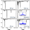 |
Fig. 3. Doublet-search statistics for the six new Blazhko detections in the Kepler data. Insets show the DFT spectra of the prewhitened data in the close neighborhood of the fundamental mode frequency f0 (horizontal axes are relative to f0). For all panels, the vertical axes are normalized, frequencies are in [c/d]. |
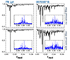 |
Fig. 4. Upper row: Same as in Fig. 3, for a new class 1 (left) and a class 2 (right) object. Lower row: Same as in the upper row, except the data were processed by annual filtering to clean the spectrum from possible instrumental effects on seasonal time scales (see text and Sect. 2). |
It may also be of interest to see the actual time series corresponding to the modulation component BLA. We recall that this time series is still a fast oscillating function with frequency components j × f0 ± k × fmod. This, together with the low amplitude, makes it difficult to find a good way to see directly the underlying signal. Using temporal Fourier fits and follow the variation of the low-order Fourier parameters (A1, φ1) is another possibility, albeit this method also suffers from some drawbacks, including the dependence on the success of the combination of quarters. Modulations are often displayed as residuals on the folded light curve, using the pulsation period as the folding period (e.g., Jurcsik et al. 2009). We opted for this method and show the corresponding plot for FN Lyr in Fig. 5. We see that the fifth-order modulation search model is a good approximation of the full BLA component, as it closely follows the observed pattern of the folded residuals.
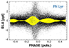 |
Fig. 5. Pulsation phase-folded residuals (X-SYS-FUN, black dots) for one of the new Blazhko variables in the Kepler data, comprising nearly 64 000 data points. The maximum light of the pulsation is at phase zero. The best-fit five-component modulation model is indicated by yellow dots. |
The relevant parameters of the six new Blazhko stars are given in Table 1. As an extension of the table notes, we add the following: The parameters were obtained by fitting a Fourier series to X-SYS, stitched quarterly. The model contains the following frequency triplets: {j × f0 − fmod, j × f0, j × f0 + fmod }, with j extending to very high harmonics, usually to ∼409. The amplitudes Atot and Amod are peak-to-peak amplitudes of the fitted fundamental and Blazhko components (FUN and BLA time series, respectively).
New Blazhko stars from the Kepler field.
5. Results: The K2 data
As described in Sect. 3, by using four different data sources for the raw photometric data, we analyzed campaign fields C01-C13 (excluding the microlensing field C09), following the RRab lists of Molnár et al. (2018) and Plachy et al. (2019). The method of analysis was the same as for the Kepler data but without the need for stitching and annual variation testing. The lack of successive campaign data on the same target, of course, requires higher levels of caution, because we have no trustworthy information as to whether a small amplitude variation on the time scale over the duration of the campaign is due to some seasonal effects or represents a real change in the star’s amplitude (even though co-trending eliminates much of the seasonal variation).
Figure 6 shows an example of the diagnostic plots obtained in the course of the analysis of the K2 data. Various data sources show different degrees of systematics. By comparing the results from these sources, we both get a better assessment of the effectiveness of the systematics filtering and a feedback on the reliability of the final classification.
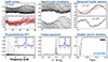 |
Fig. 6. Example of the diagnostic diagrams obtained from the K2 database. Many stars show strong systematics, such as EPIC 212457000 from field C06 shown in this figure. For a detailed description of the panels, see Fig. 2. |
A summary of the field-by-field observed occurrence rates for the various classes is given in Table 2. As a data quality parameter, in column 3 we also give the averages of the relative amplitude errors, defined (somewhat arbitrarily) as follows:
Blazhko star statistics for K2 fields.
 (2)
(2)
Here At denotes the total (peak-to-peak) fundamental mode amplitude, σ is the standard deviation of the residuals after subtracting the full triplet model (see Sect. 4), and N is the number of data points of the time series. When At is substituted by one of the low-order Fourier amplitudes (Ak in Aksin(kω + φk)), Eq. 2 gives the standard deviation (1σ error) relative to that amplitude. The true relative error for At is larger than eA/A, but this is unimportant in the present context. The inclusion of the last column – the rate of all potential Blazhko stars – is aimed at indicating the compatibility of the present survey and our earlier, more limited surveys (Kovacs 2018, 2021), where most of the class 2 objects were regarded as potential class 1 objects.
We observe a broad positive correlation between eA/A and q0 (the fraction of pure noise detections) and a negative correlation for q1 (the fraction of the Blazhko detections). This is the expected effect of noise on the outcome of the time series analysis. The class 2 objects show no correlation. This indicates a mixture of objects with and without additional signals.
The distribution of eA/A shows an approximate bimodality: eA/A > 0.0008 for the five LQ fields, whereas eA/A < 0.0006 for the seven HQ fields. Using this bimodality, for the LQ fields we obtain q1 = 0.401, whereas for the HQ set we obtain q1 = 0.535. This seems to be a significant10 difference, underscoring the effect of observational noise on the derived occurrence rates.
6. Occurrence rates
Considering only the two most important effects (noise and time base) on the detection likelihood, we find it useful to compare the Kepler and K2 results with the unique analysis of Prudil & Skarka (2017) and Skarka et al. (2020) of the Galactic Bulge RR Lyrae stars from the OGLE project. Because of the lack of strong evidence for the contrary, here we assume that the underlying distributions of the Blazhko stars are the same in the modulation frequency – modulation amplitude space, independently of the population under investigation (e.g., see Smolec 2005, on the lack of metallicity effect in the frequency of Blazhko phenomenon).
The accompanying supplementary material by Skarka et al. (2020) allows us to compare the modulation properties on a common parameter space, involving the modulation frequency, fm, and the side-lobe amplitudes, A±, relative to the full pulsation amplitudes, At11. To characterize the strength of the modulation and minimize the effect of blending, we used relative modulation amplitudes, As/At, where As = (A− + A+)/2.
In the following subsections (Sects. 6.1, 6.2, 6.3, and 6.4), we briefly review the observational support for the dependence of the observed occurrence rates on the data quality and time span. Lastly, Sect 6.5 facilitates these observations in the estimation of the underlying occurrence rate for the K2 set.
6.1. The low modulation amplitudes
First, we embarked on the distribution of the modulation amplitudes. The cumulative distribution functions (CDFs) for the three datasets are shown in Fig. 7. The Kepler set contains 24 modulated stars. The high fraction of low modulation amplitudes (33%, with As/At < 10−3) is quite remarkable. However, because the full Kepler RRab population is small, this observation carries small overall statistical weight. In comparison, while the K2 sample contains ∼23 stars (4.5%) with low modulation amplitudes, the OGLE sample has only ∼4 (0.12%). All these are in agreement with the expected trend of a decreasing number of detections with an increase of the overall noise level of the data.
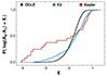 |
Fig. 7. CDF of the logarithm of the relative side-lobe amplitudes from different data sources as given in the header of the figure. While OGLE samples the Galactic Bulge, Kepler and K2 cover parts of the field. |
In a separate observation, we draw attention to the topological change in the CDF for K2 at As/At = 10−2 (X = −2), with an approximately linear decline toward smaller amplitudes. This behavior is quite different from what is observed for the OGLE sample. The change in the CDF of the K2 sample may indicate the existence of a subclass within the Blazhko stars below a critical modulation amplitude.
6.2. The long modulation periods
When considering the modulation periods, PBL, it is clear that aiming for long modulation periods with K2 is rather difficult, and, in fact, above PBL ∼ 100 d, we can only acknowledge the presence of the long-term variation. However, even this can be done with reasonably high confidence only if the modulation amplitude is large enough and the Blazhko phase is suitable at the time of the observation. Therefore, it is important to examine the fraction of long-period Blazhko stars in surveys with long baselines. With this information, we can estimate the expected number of the long-period Blazhko stars lost in the K2 data, due to the short time spans of the various campaigns.
Unlike for the modulation amplitudes, the available data in the literature on the modulation periods are fairly abundant. Including the Galactic Bulge data from OGLE, we found five extended sources covering various populations in the Galaxy and in the Large Magellanic Cloud (LMC). Table 3 summarizes the relevant data, and most importantly RL, the fraction of the long-periodic Blazhko stars to those with short modulation periods (i.e., with PBL < 100 d).
Fraction of long Blazhko periods.
The “Data” column typifies the main data acquisition method, with “literature” implying various ground-based telescopes, both individual, target-oriented projects and surveys, such as ASAS (Pojmanski 2001). The data on the LMC and those in reference [3], with some extension, were used also by Skarka et al. (2016) to investigate the modulation period distribution of 1547 RRab stars. These data yield RL = 0.471. The blind averaging of column 3 in the upper five rows yields RL = 0.517, whereas the averaging with Ntot weighting results in RL = 0.443, obviously dominated by the OGLE data. Omitting the likely specific rate for M3, simple averaging of the remaining four sources yields RL = 0.495. From these data we think that using a correction factor of RL = 0.45 − 0.50 is quite appropriate for the field RRab stars. With this factor we can estimate the long modulation period fraction in a Blazhko population if only the short modulation period population is available due to observational constraints.
6.3. The fm – Am map
In addition to the marginalized distributions, it is useful to look at the data directly on the modulation frequency (fm) – modulation amplitude (Am) plot. Although the real modulation amplitude could be several to many factors higher than the side-lobe amplitude at the fundamental frequency, both are useful for the characterization of the modulation strength. Therefore, we continue using As/At also in the maps below.
The detected Blazhko stars in the Kepler and in the twelve K2 fields are shown in Fig. 8. In comparison with the Galactic Bulge data in the background, one can observe two important differences. First, as already discussed earlier, Kepler and K2 data (the latter naturally) miss many long-period Blazhko stars. Second, not entirely unexpectedly, the Kepler and K2 data reach much deeper toward low modulation amplitudes. Another relevant result from the OGLE data is that although the survey is shallower in Am than Kepler, there does not seem to be a dependence on the modulation period. Therefore, the relative number of the detected long modulation periods (RL in Table 3) does not seem to suffer from observational bias. Furthermore, the Kepler and K2 amplitudes surpass the OGLE amplitude in both directions. We do not have an answer as to why this also occurs in the high-amplitude regime. The expected high level of deficiency of Blazhko stars with fm < 0.01 c/d from K2 is clearly exhibited.
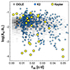 |
Fig. 8. Modulation frequency vs. relative side-lobe amplitude for the Galactic Bulge RRab inventory of the OGLE project (3141 stars from Skarka et al. 2020), plotted on a gray-scale object number density map). The 514 stars from 12 K2 fields and the 24 stars are from Kepler’s original field as detected in this paper. For comparison, there are only four stars in the OGLE sample with As/At < 0.001. |
6.4. Detection limits from signal injection
A fundamental question is whether the distribution of the amplitude modulation ends abruptly at low amplitudes, or whether it gradually decreases to zero as data precision allows for the detection of lower modulation amplitudes. In the former case, if the detection limit for a given dataset is known, one would see a clear break between the low-end of the distribution of Am and the detection limit. In a very preliminary way, we considered this question by performing injected signal tests in the Kepler and K2 data.
Begining with the raw input fluxes {Xi}, we generated injected fluxes {Zi} by modifying {Xi} according to the following formulae;
 (3)
(3)
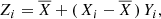 (4)
(4)
where {Yi} is the modulation signal at the i-th data item, Amod is the total modulation amplitude (different from the side-lobe modulation amplitude As/At), fmod is the modulation frequency, and  is the robust average of {Xi}. Importantly, these modified fluxes go through the same steps (including systematics filtering) as the other, non-modified input time series (see Sect. 2). For any given injected time series at fixed fmod and t0, we looked for a proper value of Amod to reach the detection limit (the minimum of Amod at which the detection becomes secure, based on the diagnostics described in Sect. 2). With this Amod, the analysis yields also the corresponding As/At, that can be compared with the observed values derived for the Blazhko stars.
We selected non-Blazhko stars (class 0 and 2 stars) both from the Kepler set (12 stars) and from field C08 of K2 (17 stars). The Kepler set was tested at two modulation frequencies to investigate the detection sensitivity to long and short modulation periods (the former is to aid our understanding of the apparent lack of more long-period Blazhko stars in the Kepler set).
Figure 9 delivers the following, partially expected results for the Kepler data12. For the short-period injected signals, the detection limits are close to the range of the low-amplitude Blazhko stars and also to the formal modulation amplitudes of the non-Blazhko stars (shown as yellow circles in Fig. 9; see also footnote 12). This implies a continuous spectrum of modulation amplitudes down to the detection limit (i.e., no sign of an abrupt stop to the Blazhko phenomenon below a critical modulation amplitude). For the modulation period approximately covering 2.5 quarters, naturally, we have a higher detection limit, but still low-enough to reach Blazhko stars (even though this is a low-populated region according to the OGLE Bulge data). Although this may imply that the available small sample of RR Lyrae stars in the Kepler field indeed lacks a sufficient number of long-period Blazhko stars, it is important to recall that several stars are affected by annual variations (see Sects. 2, 4) that may blur the long-period modulation. In any case, the hidden long-period Blazhko stars in the Kepler sample must have considerably lower modulation amplitudes than their counterparts in the Galactic Bulge.
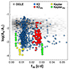 |
Fig. 9. Class 0 and 2 (i.e., non-Blazhko) stars from Kepler and K2 on the modulation frequency – relative side-lobe amplitude diagram (see footnote 12). For comparison, the Galactic Bulge Blazhko map is replotted. Also shown are the injection tests to assess detection efficacy. We used the non-Blazhko stars with the following injected modulation frequencies: fm = 0.004 and 0.03 c/d for Kepler and fm = 0.025 for C08 of K2. The K2 injected result is plotted for all the available data sources (i.e., there are multiple points for the same object). |
The K2 data obviously indicate a higher detection limit, but again in agreement with the low-amplitude tail of the detected modulations. For the first sight, the size of the scatter in the detected modulation frequencies seems to be unexpected. However, considering the overall length of a campaign (∼80 days), the line widths of the peak profiles of the frequency spectra are in the range of ∼0.01 c/d. Therefore, considering that these signals are at the detection limits, the observed scatter is not surprising.
6.5. Underlying occurrence rates
If we dismiss the sensitivity of the detection on the noise level (which is obviously incorrect), we can get a lower limit for the true number of Blazhko stars by simply considering the ratio between the short and long Blazhko periods as derived in Sect. 6.2 from samples, apparently complete in PBL. In the K2 fields, we find 514 Blazhko stars. From these 36 have PBL > 100 d. With a total number of 1061 RRab stars in the sample and using a long-period boosting factor 0.45 (see Sect. 6.2), we arrive at a rate of (514 − 36)×1.45/1061 = 0.653 (or to 0.676 if we use – a still likely – factor of 1.50).
For a better guess, we need to consider the fact that certain modulated stars might remain hidden even if PBL < 100 d simply because of the high noise level in cases when the modulation amplitudes are low. Pursuing this deeper assessment of the underlying rate, we essentially follow the method described in our former papers (Kovacs 2018, 2021, 2022). In principle, this is a simple Monte Carlo (MC) simulation, by using the available “best guesses” on the distributions of the modulation periods and modulation amplitudes. Here, we rely on the As/At distribution derived in this study from the analysis of 12 fields from K2 and the distribution for PBL, as given by the OGLE data for the Galactic Bulge (Skarka et al. 2020).
With the corresponding CDFs, we can assign modulation frequencies to each member of the sample and inject modulation signals in the observed fluxes (in the same way as described in Sect. 6.4, except if the known Blazhko stars were included in the simulation in which case we would need to prewhiten their fluxes from the Blazhko component). This is obviously a formidable task, considering the large number of stars and the large number of randomly selected (fm, Am) pairs needed for statistical stability. Instead, we can use a simplified method (similar to those in our earlier studies), enabling a fairly accurate assessment of the detectability of a sinusoidal signal in the presence of noise.
To estimate the detection limit from the noise of the signal, we would then relate the relative amplitude error eA/A (see Eq. 2 in Sect. 5) to the relative side-lobe amplitudes, As/At. We recall that eA/A is given for all stars, due to the frequency analysis performed during the survey. We plot the detected side-lobe amplitudes as a function of the amplitude error in the left panel of Fig. 10. Although the correspondence is not entirely flawless, the 6σ criterion seems to be a reasonable detection limit: nearly all class 1 and 2 objects fall above this detection limit, whereas a considerable number of the class 0 objects fall below13. The intermingling of class 1 and 2 objects is also expected, because the latter do have Fourier signals. Nevertheless, their origin is unclear from the available data.
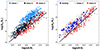 |
Fig. 10. Left: Relative amplitude error (see Fig. 2) vs. relative side-lobe amplitudes for the 1061 RRab stars from 12 K2 fields. The straight line corresponds to As/At = 6 × eA/A, which we identify as the 6σ detection limit in this paper. Right: Injected signal test for the 17 class 0 and class 2 stars in C08 of K2 (blue points). As in Fig. 9, we plot the results for all data sources used in the signal injection test. |
It is also useful to check the performance of the above detection criterion for injected signals, where the analysis is performed independently of this criterion, relying entirely on the diagnostics described in Sect. 2. Using the same test result for the K2 field C08 as in Sect. 6.4, we obtain the plot shown in the right panel of Fig. 10. Again, the 6σ condition looks valid, even though it was not used in tuning the injected amplitudes to the detectability. Furthermore, as partially expected, the detections cover the “gray area” of class 2 objects with Fourier detection flags but in the low- and/or mid-S/N regime.
Briefly, the search for the underlying occurrence rate that yields the best-matching predicted rate to the one observed is built on the following core loop. First, we randomly assign modulation status to N1 members of the whole population of N objects. Those with single-mode status (N − N1 stars) are no longer dealt with in this particular loop. Next, based on the CDFs chosen for the generation of the modulation parameters, (fm, Am) pairs are randomly assigned to the N1 stars. Then, from the noise-detection relation described above, the detection status can be determined due to the knowledge of the star-by-star value of the observed relative noise level eA/A. Next, the detections with short modulation periods (i.e., those with assigned fm greater than a fixed lower limit of fmmin) are counted, and their number is registered as detections in the particular realization.
The whole loop described above is repeated for an ample amount of times (in our case 500 times). The derived number of detections in the ir-th realization, Ndet(ir), is used together with the values from the other realizations to compute the average and standard deviation of the predicted observable rate of short-period modulated stars for the assumed underlying rate of the full population of modulated stars (i.e., including those with fm < fmmin). The underlying rate is tuned until the observed and predicted rates match.
Following a conservative approach, we first use the PBL distribution of the Bulge sample (although it yields a lower rate boost than expected for the field stars) and native (i.e., derived from the K2 sample) modulation amplitude distribution (although the CDF derived from the Kepler data suggest a considerably higher boost).
Table 4 summarizes the result for the K2 data. The short modulation period rates, Qobss, were matched with the predicted values within ±0.002. The overall boost in the Qobss rates is 59%, shared between the boost from accounting for the loss of class 1 objects due to noise (a boost with a factor of 1.15) and the boost from missing long-period modulations (a boost by a factor of 1.38, since we used the Galactic Bulge sample to constrain the ratio of the long modulations). Using these factors, we can perform a brief sanity check of the derived underlying rates. For the full K2 dataset, the number of detections with short modulation periods is 514 − 36 = 478. Considering the boost due to noise bias gives 478 × 1.15 = 550. Finally, the long-period bias yields: 550 × 1.38/1061 = 0.715, closely similar to what is shown in the third line of Table 4.
Underlying occurrence rates for K2.
The above simple estimation can be extended to consider more realistic boost factors for the loss of long modulation periods. Using the lower value of 1.45 from the preferred range of the modulation period bias factor (Sect. 6.2) and maintaining the moderate boost used above for debiasing the noise effect, we get 550 × 1.45/1061 = 0.752 for the full K2 set discussed above.
Although the Kepler set has rather moderate statistical weight, it is still interesting to test the effect of changing the CDF from K2 for the modulation amplitude to the one derived from the Kepler set (see Fig. 7). From the MC simulation, we obtain a factor of ∼1.5 for noise debiasing. This factor, and the boost for the long modulation periods derived from the field stars yield a rate of 478 × 1.50 × 1.45/1061 = 0.980. A more sensible (albeit ad hoc) noise boosting factor of 1.25 yields a rate of 0.82. We conclude that the current data for the K2 RRab sample support an underlying Blazhko occurrence rate of 75% or higher.
7. Conclusions
In this paper, we aimed at: (i) a deep analysis of the RRab stars in the Kepler field, which offers a unique dataset to investigate these variables at the 100 ppm level; (ii) extending the analysis to twelve K2 fields to compensate for the issues arising from the small sample size and, more importantly, from the high level of crowdedness in the Kepler field; and (iii) revisiting the question of the modulation amplitude distribution and the true occurrence rate of the Blazhko phenomenon. Concerning the last point, it is important to note that apparently none of the studies dealing with the occurrence rate of the Blazhko phenomenon are concerned much with observational biases, whereas these profoundly affect the number of detections.
In the present work, there are several important ingredients that differ from our earlier studies on the statistics of the Blazhko phenomenon (Kovacs 2018, 2021, 2022). The following is the list of the new features of the analysis presented in this paper:
-
We relied on the observed fraction of long modulation periods (from other surveys) and did not attribute every remnant Fourier peak near the fundamental mode to the effect of long-term modulation (as we largely did in our earlier studies).
-
For the K2 analysis, we used up to four independent data sources, thereby greatly increasing the reliability of the detection.
-
We used codes of higher sophistication, enabling us to perform better filtering of instrumental systematics and used various complimentary methods to search for light curve modulation.
-
We used a three-level modulation classification scheme, where significant peaks in the frequency spectra count only if they are accompanied by other supporting diagnostics.
The main results of this paper can be summarized as follows:
-
Although the Kepler data on RR Lyrae stars is at the highest standards both in length and quality, the high crowding and the accompanying instrumental effects make it difficult to aim at long-period Blazhko modulations at the ppt level or lower.
-
Despite the main obstacle above, we find six new Blazhko stars in the Kepler field with modulation periods of less than ∼100 d and side-lobe amplitudes around 250 ppm (for five stars). The considerable fraction (5/24) of such low-amplitude Blazhko stars serves as a warning that other, shallower surveys may miss a non-negligible fraction of the Blazhko population.
-
From the literature, which covers various RR Lyrae populations and instrumentation, we find that the relative number of Blazhko stars with long modulation periods (i.e., with PBL > 100 d) is very high. In the overall sense, there are half as many Blazhko stars in the long-period regime than in the short-period regime. This again is a warning sign for the short-term surveys when counting the Blazhko population. (e.g., works based on the non-continuous viewing sectors of the TESS satellite – Molnár et al. 2022).
-
From the analysis of 1061 RRab stars in 12 K2 fields, we obtain an observed occurrence rate of 48%, which, after correction for biases by the finite observational time base and noise, increases to 75%. This is our best (although still conservative) estimate for the underlying occurrence rate of Blazhko RRab stars in the Galactic field.
-
Based on the analysis of the Kepler and K2 data, the modulation amplitudes do not seem to exhibit a minimum value; there are modulations close to the detection limits in both datasets, continuously extending the distribution to very low amplitudes.
The actual physical implementation is realized by a stand-alone Fortran code, relying only on the publicly available raw photometric time series.
If not stated otherwise, the word “prewhitened” refers to the data and the spectra obtained after subtracting the fundamental mode FUN from the systematics-filtered data X-SYS.
This is slightly an “over safe” condition, because the doublet search method (see later) is, in general, more sensitive to modulation components due to power accumulation from several harmonics. The DFT yields information only separately on these components, and therefore, the signal-to-noise ratio (S/N) is smaller.
Although the orbital period of the Kepler satellite is slightly longer than that of the Earth, using the latter does not cause any appreciable difference.
That is, a close component to the fundamental mode, with a frequency difference of less than ∼0.15 c/d (we note that very few objects fall in the frequency interval of 0.10 − 0.15 c/d).
Because of the very high data quality, leakage to the low frequency regime may occur from components well above the Nyquist frequency, from the very high harmonics of the fundamental mode frequency f0. This can be avoided by a sufficiently high-order Fourier fit of FUN.
By using Eq. (1) of Alcock et al. (2003) for the sampling error – assuming Poisson distribution – we find that the difference between the two rates is significant above the 4 sigma level.
For the Galactic Bulge data, At = (AmeanMIN + AmeanMAX)/2 from Table 1 of Skarka et al. (2020).
Because of the absence of modulation signals surpassing the detection criteria for class 0 and 2 objects, the plotted quantities are simply those associated with the highest side peaks near the fundamental frequency.
The large jamming of class 0 objects above the detection limit at high noise level is due to C07, the noisiest field. By leaving out this field, the separation of the class 0 objects becomes far more favorable.
Acknowledgments
We thank József Benkő for drawing our attention to an earlier note on the Blazhko classification of V346 Lyr. We appreciate Marek Skarka’s quick response on the parameterization of the OGLE’s Bulge RR Lyrae sample. We thank Eric Petigura, Andrew Vanderburg and Rodrigo Luger for answering questions related to data accessibility. The quick and instructive report of the referee is acknowledged. This paper includes data collected by the Kepler mission and obtained from the MAST data archive at the Space Telescope Science Institute (STScI). Funding for the Kepler mission is provided by the NASA Science Mission Directorate. STScI is operated by the Association of Universities for Research in Astronomy, Inc., under NASA contract NAS 5-201326555.
References
- Alcock, C., Alves, D. R., Becker, A., et al. 2003, ApJ, 598, 597 [NASA ADS] [CrossRef] [Google Scholar]
- Bakos, G. Á., Torres, G., Pál, A., et al. 2010, ApJ, 710, 1724 [NASA ADS] [CrossRef] [Google Scholar]
- Benkő, J. M., & Szabó, R. 2015, ApJ, 809, L19 [CrossRef] [Google Scholar]
- Benkő, J. M., Plachy, E., Szabó, R., et al. 2014, ApJS, 213, 31 [CrossRef] [Google Scholar]
- Benkő, J. M., Jurcsik, J., & Derekas, A. 2019, MNRAS, 485, 5897 [CrossRef] [Google Scholar]
- Blazhko, S. 1907, Astron. Nachr., 175, 325 [NASA ADS] [CrossRef] [Google Scholar]
- Bódi, A., Szabó, P., Plachy, E., et al. 2022, PASP, 134, 4503 [Google Scholar]
- Borucki, W., Jr 2017, PAPhS, 161, 38B [Google Scholar]
- Deeming, T. J. 1975, Ap&SS, 36, 137 [Google Scholar]
- Forró, A., Szabó, R., Bódi, A., et al. 2022, ApJS, 260, 20 [CrossRef] [Google Scholar]
- Greer, P. A., Payne, S. G., Norton, A. J., et al. 2017, A&A, 607, A11 [NASA ADS] [CrossRef] [EDP Sciences] [Google Scholar]
- Howell, S. B., Sobeck, C., Haas, M., et al. 2014, PASP, 126, 398 [Google Scholar]
- Jurcsik, J. 2019, MNRAS, 490, 80 [Google Scholar]
- Jurcsik, J., Sódor, Á., Szeidl, B., et al. 2009, MNRAS, 400, 1006 [NASA ADS] [CrossRef] [Google Scholar]
- Kovacs, G. 2018, A&A, 614, L4 [NASA ADS] [CrossRef] [EDP Sciences] [Google Scholar]
- Kovacs, G. 2021, ASPC, 529, 51 [Google Scholar]
- Kovacs, G. 2022, VMSAI, 2, 24 [Google Scholar]
- Kovacs, G., Bakos, G., & Noyes, R. W. 2005, MNRAS, 356, 557 [CrossRef] [Google Scholar]
- Luger, R., Agol, E., Kruse, E., et al. 2016, AJ, 152, 100 [Google Scholar]
- Luger, R., Kruse, E., Foreman-Mackey, D., et al. 2018, AJ, 156, 99 [Google Scholar]
- Molnár, L., Plachy, E., Juhász, Á. L., et al. 2018, A&A, 620, A127 [NASA ADS] [CrossRef] [EDP Sciences] [Google Scholar]
- Molnár, L., Bódi, A., Pál, A., et al. 2022, ApJS, 258, 8 [CrossRef] [Google Scholar]
- Moskalik, P., & Poretti, E. 2003, A&A, 398, 213 [NASA ADS] [CrossRef] [EDP Sciences] [Google Scholar]
- Nemec, J. M., Smolec, R., Benkő, J. M., et al. 2011, MNRAS, 417, 1022 [NASA ADS] [CrossRef] [Google Scholar]
- Petigura, E. A., Schlieder, J. E., Crossfield, I. J. M., et al. 2015, ApJ, 811, 102 [Google Scholar]
- Plachy, E., & Szabó, R. 2021, Front. Astron. Space Sci., 7, 81 [NASA ADS] [CrossRef] [Google Scholar]
- Plachy, E., Molnár, L., Bódi, A., et al. 2019, ApJS, 244, 32 [CrossRef] [Google Scholar]
- Pojmanski, G. 2001, ASPC, 246, 53 [Google Scholar]
- Press, W. H., Teukolsky, S. A., Vetterling, W. T., et al. 1992, Numerical Recipes in Fortran 77. The Art of Scientific Computing, 2nd edn., 1992 [Google Scholar]
- Prudil, Z., & Skarka, M. 2017, MNRAS, 466, 2602 [NASA ADS] [CrossRef] [Google Scholar]
- Shapley, H. 1916, ApJ, 43, 217 [Google Scholar]
- Skarka, M., Liska, J., Auer, R. F., et al. 2016, A&A, 592, A144 [NASA ADS] [CrossRef] [EDP Sciences] [Google Scholar]
- Skarka, M., Prudil, Z., & Jurcsik, J. 2020, MNRAS, 494, 1237 [NASA ADS] [CrossRef] [Google Scholar]
- Smith, J. C., Stumpe, M. C., Van Cleve, J. E., et al. 2012, PASP, 124, 1000 [Google Scholar]
- Smolec, R. 2005, Acta Astron., 55, 59 [NASA ADS] [Google Scholar]
- Szeidl, B. 1988, in Multimode Stellar Pulsations, eds. G. Kovács, L. Szabados, & B. Szeidl (Budapest: Konkoly Observatory, Kultura), 45 [Google Scholar]
- Szeidl, B., & Kolláth, Z. 2000, ASPC, 203, 281 [Google Scholar]
- Tamuz, O., Mazeh, T., & Zucker, S. 2005, MNRAS, 356, 1466 [Google Scholar]
- Vanderburg, Andrew, & Johnson, John Asher 2014, PASP, 126, 948 [NASA ADS] [CrossRef] [Google Scholar]
All Tables
All Figures
|
Fig. 1. Brief summary of the time series procedures employed in this work to search for modulated RR Lyrae stars. The prefix “w” in wFit denotes a weighted least squares fit, controlled by the outlier array, generated during the fitting cycle. Additional details can be found in Sect. 2. |
| In the text | |
|
Fig. 2. Example of diagnostic diagrams for an RR Lyrae star from the Kepler field, used in search for modulated stars. Upper row, from left to right: Systematics-corrected (upper subpanel) and raw light curves; units on the horizontal and vertical axes are in days and relative magnitudes, respectively. Close-up of the lower and upper parts (respectively, upper and lower halves of the panel) of the filtered light curve shown in the first panel (units are the same as in the first panel). Variation (relative to the average) of the time-dependent Fourier parameters at the fundamental frequency f0. The red line indicates the linear regression to ΔA1(t). Vertical axis units: [ppt] and [rad]. Lower row, from left to right: Full DFT of the prewhitened data, with the inset zooming on the region of f0 (the horizontal axis shows f − f0). Folded spectrum, with a similar plot structure as in the previous panel. RMS values of the doublet search at various modulation frequencies. The KIC ID (also known as V1510 Cyg) is shown in the lower right corner. All vertical axes are normalized to the peak values; horizontal axes have the same units (i.e., [c/d]). See Sect. 2 for additional details. |
| In the text | |
|
Fig. 3. Doublet-search statistics for the six new Blazhko detections in the Kepler data. Insets show the DFT spectra of the prewhitened data in the close neighborhood of the fundamental mode frequency f0 (horizontal axes are relative to f0). For all panels, the vertical axes are normalized, frequencies are in [c/d]. |
| In the text | |
|
Fig. 4. Upper row: Same as in Fig. 3, for a new class 1 (left) and a class 2 (right) object. Lower row: Same as in the upper row, except the data were processed by annual filtering to clean the spectrum from possible instrumental effects on seasonal time scales (see text and Sect. 2). |
| In the text | |
|
Fig. 5. Pulsation phase-folded residuals (X-SYS-FUN, black dots) for one of the new Blazhko variables in the Kepler data, comprising nearly 64 000 data points. The maximum light of the pulsation is at phase zero. The best-fit five-component modulation model is indicated by yellow dots. |
| In the text | |
|
Fig. 6. Example of the diagnostic diagrams obtained from the K2 database. Many stars show strong systematics, such as EPIC 212457000 from field C06 shown in this figure. For a detailed description of the panels, see Fig. 2. |
| In the text | |
|
Fig. 7. CDF of the logarithm of the relative side-lobe amplitudes from different data sources as given in the header of the figure. While OGLE samples the Galactic Bulge, Kepler and K2 cover parts of the field. |
| In the text | |
|
Fig. 8. Modulation frequency vs. relative side-lobe amplitude for the Galactic Bulge RRab inventory of the OGLE project (3141 stars from Skarka et al. 2020), plotted on a gray-scale object number density map). The 514 stars from 12 K2 fields and the 24 stars are from Kepler’s original field as detected in this paper. For comparison, there are only four stars in the OGLE sample with As/At < 0.001. |
| In the text | |
|
Fig. 9. Class 0 and 2 (i.e., non-Blazhko) stars from Kepler and K2 on the modulation frequency – relative side-lobe amplitude diagram (see footnote 12). For comparison, the Galactic Bulge Blazhko map is replotted. Also shown are the injection tests to assess detection efficacy. We used the non-Blazhko stars with the following injected modulation frequencies: fm = 0.004 and 0.03 c/d for Kepler and fm = 0.025 for C08 of K2. The K2 injected result is plotted for all the available data sources (i.e., there are multiple points for the same object). |
| In the text | |
|
Fig. 10. Left: Relative amplitude error (see Fig. 2) vs. relative side-lobe amplitudes for the 1061 RRab stars from 12 K2 fields. The straight line corresponds to As/At = 6 × eA/A, which we identify as the 6σ detection limit in this paper. Right: Injected signal test for the 17 class 0 and class 2 stars in C08 of K2 (blue points). As in Fig. 9, we plot the results for all data sources used in the signal injection test. |
| In the text | |
Current usage metrics show cumulative count of Article Views (full-text article views including HTML views, PDF and ePub downloads, according to the available data) and Abstracts Views on Vision4Press platform.
Data correspond to usage on the plateform after 2015. The current usage metrics is available 48-96 hours after online publication and is updated daily on week days.
Initial download of the metrics may take a while.