| Issue |
A&A
Volume 699, July 2025
|
|
|---|---|---|
| Article Number | A345 | |
| Number of page(s) | 11 | |
| Section | Celestial mechanics and astrometry | |
| DOI | https://doi.org/10.1051/0004-6361/202555160 | |
| Published online | 22 July 2025 | |
Validating the bright Gaia celestial reference frame with new VLBI astrometry of radio stars
1
Shanghai Astronomical Observatory, Chinese Academy of Sciences,
80 Nandan Road,
Shanghai
200030,
PR China
2
University of Chinese Academy of Sciences,
No. 19 (A) Yuquan Rd, Shijingshan,
Beijing
100049,
PR China
3
Korea Astronomy and Space Science Institute,
776 Daedeok-daero,
Yuseong-gu,
Daejeon
34055,
Republic of Korea
4
University of Helsinki,
PO Box 64,
Helsinki
00014,
Finland
★ Corresponding author: This email address is being protected from spambots. You need JavaScript enabled to view it.
Received:
15
April
2025
Accepted:
20
June
2025
Abstract
Aims. There exist inconsistencies between the bright and faint Gaia Celestial Reference Frame 3 (Gaia-CRF3), which manifests as a systematic rotation and needs to be independently estimated then corrected in future data releases.
Methods. We collected 64 radio stars with very long baseline interferometry (VLBI) astrometry, of which 16 have new VLBI observations with reference epochs close to Gaia. We estimated the orientation and spin biases of the bright Gaia-CRF3 by comparing VLBI radio star astrometry with their Gaia DR3 counterparts. We also attempted to estimate orientation by utilizing the a priori magnitude-dependent spin parameters derived from Gaia’s internal estimations.
Results. Our independent estimation of the orientation at G < 10.5 is [−15 ± 119, +330 ± 139, +218 ± 109] μas (J2016.0), and the spin ([+21 ± 18, +52 ± 20, −7 ± 20] μ μas yr−1) agrees with Gaia’s internal estimation within a 1σ range. The orientation-only estimation suggests that the orientation bias of the bright Gaia-CRF3 may also be magnitude-dependent.
Key words: astrometry / reference systems / stars: kinematics and dynamics
© The Authors 2025
 Open Access article, published by EDP Sciences, under the terms of the Creative Commons Attribution License (https://creativecommons.org/licenses/by/4.0), which permits unrestricted use, distribution, and reproduction in any medium, provided the original work is properly cited.
This article is published in open access under the Subscribe to Open model. This email address is being protected from spambots. You need JavaScript enabled to view it. to support open access publication.
1 Introduction
The Gaia mission (Gaia Collaboration 2016) provides precise astrometry for 1.8 billion sources in its latest data release, Gaia DR3 (Gaia Collaboration 2023), and established its celestial reference frame, Gaia-CRF3 (Gaia Collaboration 2022), based on an extragalactic source (quasar) sample of 1.6 million. However, most quasars are faint in the optical band, the G-band magnitude of which ranges from 13 to 21, without coverage of the bright end (G < 13). This may result in potential inconsistency at the bright end. Unfortunately, evidence suggests that this inconsistency exists and manifests as a systematic rotation (orientation bias at reference epoch and spin with time) (Lindegren et al. 2018; Brandt 2018). The origin of this rotation may be astrometric instrument calibration limitations, such as window class effects (Lindegren 2020).
The rotation can be estimated internally within Gaia or through a comparison with the Hipparcos catalog (van Leeuwen 2007). For example, Cantat-Gaudin & Brandt (2021) estimated spin parameters with samples collected from known binaries and open clusters, and an ad hoc correction is applied in the astrometric solution of Gaia DR3 based on a comparison of proper motions with Hipparcos (Lindegren et al. 2021b).
It is necessary to validate the above estimations with independent external methods. For example, very long baseline interferometry (VLBI) astrometry of radio stars is a direct approach for the validation (Malkin 2016). Gaia-CRF3 is aligned to the International Celestial Reference Frame 3 (ICRF3, Charlot et al. 2020) using common quasars at the faint end. Although there are still inconsistencies in a small number of common quasars (Charlot 2025), the overall alignment uncertainty is about 7 μ as (Gaia Collaboration 2022). Since VLBI astrometry of radio stars is on an ICRF base, a comparison between VLBI and Gaia astrometry of radio stars can give an estimation of orientation and spin parameters between the bright and faint end of Gaia-CRF. There have been several related works, such as Lindegren (2020), Bobylev (2022), Lunz et al. (2023), Lunz et al. (2024), and Zhang et al. (2024), but the small sample size of available radio stars limits the reliability of their results.
In our previous studies, we observed 16 radio stars in total with the Very Long Baseline Array (VLBA), which significantly expanded the available radio star sample (Chen et al. 2023; Jiang et al., in prep.; Zhang et al., in prep.). In this paper, we present a new CRF alignment result based on radio stars, integrating historical data with our new data. The data we use are introduced in Sect. 2. Sect. 3 describes the methods and results of the CRF alignment. We sum up in Sect. 4.
2 Data
2.1 VLBI data
The VLBI data used in this study consist of two parts: historical data and our new data. Lindegren (2020) collected 41 radio stars that have both VLBI parallaxes and proper motions and full astrometry in Gaia DR2. However, some of the data are old and the positions of their calibrators are out of date. Lunz et al. (2023) transferred these positions to the latest ICRF3, and provided new one-epoch VLBA observations of 32 radio stars (in which one is fainter than G = 13, and therefore not used in this study). We included all these data in our dataset for this study. In Chen et al. (2023), Jiang et al. in prep., and Zhang et al., in prep., we provide VLBI astrometry of 2, 3, and 11 radio stars, respectively. These data include 15 stars with full five-parameter astrometry and 1 with two one-epoch observations, and are all included in our dataset. All historical and new VLBI data are listed in Appendix A, including 64 radio stars. Note that some stars have multiple data sources (e.g., we reobserved several “old” stars).
2.2 Gaia data
We collected Gaia counterparts of our VLBI samples, all of which have full five-parameter astrometry in Gaia DR3, and their G magnitudes range from 4.5 to 13. The parallax zero-point problem of Gaia DR3 may affect the usage of one-epoch VLBI data, so we corrected it using the recipe provided by Lindegren et al. (2021a), with coefficients given by Ding et al. (2024).
3 Estimation of the rotation between the bright Gaia-CRF3 and ICRF3
3.1 Solution of both orientation and spin parameters
We applied the CRF alignment solution method introduced in Sect. 2 of Zhang et al. (2024) to the radio star dataset. In simple terms, we assumed that there exists a timedependent rotation between the bright Gaia-CRF3 and ICRF3, and that it can be described with a set of six parameters x = [εX(T), εY(T), εZ(T), ωX, ωY, ωZ]′, of which the first three parameters describe an orientation bias at reference epoch T = J2016.0, while the last three parameters describe a spin at a constant angular velocity (or: the time derivative of orientation). This rotation can be estimated from the differences between VLBI and Gaia astrometry of the same sources. Because the rotation is on a small scale (hundreds of microarcseconds for orientation and tens of microarcseconds per year for spin), a linear approximation satisfies the need for accuracy, and we applied the least-square method to solve the parameters.
Not all radio stars are suitable for the CRF alignment solution, for different reasons, such as the intrinsic physical properties of the stars. For these stars, there may exist quite large differences between VLBI and Gaia astrometry, which will interfere with the estimation of CRF rotation. To eliminate these radio stars with high loss (outliers), we applied a similar iteration procedure to the one Lindegren (2020), Lunz et al. (2023), Zhang et al. (2024), and Lunz et al. (2024) used. The solution was first applied to the entire dataset (0 < G < 13) including m = 64 stars, then the star i(i = 1 … m) with the highest loss (Qi / vi., normalized by the dimension of VLBI data) was rejected and the solution was applied again to the remaining stars. The iteration was repeated for k = 0, 1, … rejected stars. The evolutions of max (Qi / vi), reduced chi-square ( ), and estimated rotation parameters are shown in Figure 1.
In the initial rounds of iteration, due to the influence of outliers,  is very large and the rotation parameters also change drastically. As k increases,
  and rotation parameters decrease and tend to be stable, and the max Qi / vi drops below 30 when k = 19, at which time the maximum in the remaining samples is 26.18 (VY CMa). The rotation parameters also keep stable between k = 17 and 21, so we adopted the result at k = 17 for the solution, with a remaining accepted star number of l = 47 and
  , as is shown in Table 1. Compared to the results of Lunz et al. (2024), the uncertainties of the parameters are improved by roughly 50% and 30% in orientation and spin, respectively, benefitting from the additional VLBI data.
However, systematic inconsistencies do not only exist between magnitudes above and below G = 13 in Gaia DR3. As is shown in Fig. 4 of Cantat-Gaudin & Brandt (2021) and Fig. 20 of Lindegren et al. (2021a), both proper motion and parallax biases are not stable between G = 10.5 and 13. The magnitude dependency may explain why the result of solution 0 < G < 13 does not agree very well with that of Lunz et al. (2024), especially in orientation parameters. The new astrometry we added changes the magnitude distribution of the radio star sample, and due to the epochs being close to the Gaia reference epoch, the new data have a high weight in the orientation estimation, which has a great impact on the result.
Internal estimations of the relationships between CRF spin and G magnitude can be conducted by dividing binary and open cluster samples into multiple magnitude bins, but the number of VLBI radio star samples is too small to do so. Therefore, we tried to solve rotation parameters with a magnitude limit of G < 10.5, and the remaining star number is 50. A similar iteration was conducted (iteration shown in Appendix B, statistics shown in Appendix C), and we adopted the result at k = 13 for the solution, with a remaining star number of l = 37 and  .
.
The results of solution 0 < G < 10.5 are also listed in Table 1 and agree well with Cantat-Gaudin & Brandt (2021): the spin parameters are within a 1σ range of the internal estimation at G < 10.5. The agreement between internal and external estimations is quite satisfying and is strong proof of the existence of systematic rotation between the bright and faint (quasar-based) Gaia-CRF3 (which is precisely aligned with ICRF3).
3.2 Solution of orientation parameters only
We noticed that the discrepancies in orientation parameters between solution 0 < G < 13 and 0 < G < 10.5 are much beyond 1σ, and so we conducted further investigations into it. It is necessary to fix spin parameters, then we can study orientation parameters independently. Since the spin parameters of solution G < 10.5 agree well with Cantat-Gaudin & Brandt (2021), we tend to accept that their results are reliable. We therefore tried to solve orientation parameters with spin parameters from Cantat-Gaudin & Brandt (2021, Table 1) as a priori values. This approach has several advantages:
A priori values are given as a set of spin parameters for each of the 12 magnitude bins, which better reflects reality than using a set of magnitude-independent spin parameters;
Only three orientation parameters need to be solved in the solution, reducing the negative impact of the limited sample size;
Similar to (2), now we can try to solve for several magnitude bins to examine the relationship between CRF orientation and the G magnitude.
The mathematical form of the solution needs to be slightly modified; this is introduced in Appendix E. We solved for 0 < G < 13, 0 < G < 10.5, and 10.5 < G < 13, respectively. The sky distribution of the samples is shown in Appendix D, and the results are listed in Table 1. As is shown in Fig. 2, the results show that the orientation parameters change with G magnitude, which suggests that the orientation bias of the bright Gaia-CRF3 may also be magnitude-dependent. However, due to the limited sample size of each bin (especially 10.5 < G < 13), the uncertainties are relatively large. The results may also be biased by systematic offsets of some samples; for example, radio-optical offsets of the stars or position errors of calibrators. Therefore, additional VLBI astrometry of radio stars is essential to achieve more robust and conclusive results.
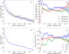 |
Fig. 1 Evolution of loss and rotation parameters with rejected star number, k, increasing in the full dataset (0 < G < 13). (a) Max Qi(x) in the solution (star names labeled). (b) |

Results of CRF alignment solution.
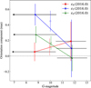 |
Fig. 2 Orientation-magnitude relationship of orientation-only solutions. Hollow markers denote the solution 0 < G < 13. Markers are horizontally shifted by 0.05 to avoid error bars overlapping. Horizontal lines of markers represent their magnitude range. |
4 Summary
We have given an external estimation of the orientation and spin biases of the bright Gaia-CRF3 by comparing VLBI radio star astrometry and their Gaia DR3 counterparts. We collected all available VLBI astrometry for 64 radio stars, including historical and new observations, and found:
Our external estimation of spin parameters at G < 10.5 ([+21 ± 18, +52 ± 20,−7 ± 20] μ as yr−1) agrees with Gaia’s internal estimation (binaries and open clusters, Cantat-Gaudin & Brandt 2021) within a 1σ range;
Taking spin parameters from the internal estimation as a priori values, our estimation of the orientation parameters suggests that the orientation bias of the bright Gaia-CRF3 may also be magnitude-dependent.
External estimation with radio stars is now the only way to determine the orientation of the bright Gaia-CRF. Our analysis demonstrates that the orientation in the bright-end Gaia-CRF samples exhibits a possible magnitude dependency. While the present sample size of 11 stars in the range of 10.5 < G < 13 provides a foundational insight, it underscores the need for additional radio stars with VLBI astrometry. Drawing parallels from the Gaia parallax zero-point, which is known to vary with G magnitude, color, sky position, and other potential factors, we emphasize the importance of a more even sky distribution and covering different magnitudes uniformly in future observations. Such efforts are expected to not only refine uncertainties in parameter estimation but also enable optimized binning strategies and mitigate potential selection biases.
Acknowledgements
The Python code for CRF link is available at Zhang (2025). This work is supported by the National Natural Science Foundation of China (NSFC) under grant Ns. U2031212, the National Key R&D Program of China (No. 2024YFA1611500), and the Strategic Priority Research Program of the Chinese Academy of Sciences, Grant No. XDA0350205. This work has made use of data from the European Space Agency (ESA) mission Gaia (https://www.cosmos.esa.int/gaia), processed by the Gaia Data Processing and Analysis Consortium (DPAC, https://www.cosmos.esa.int/web/gaia/dpac/consortium). Funding for the DPAC has been provided by national institutions, in particular the institutions participating in the Gaia Multilateral Agreement. The Gaia services (https://gaia.ari.uni-heidelberg.de/index.html) provided by the Astronomisches Rechen-Institut (ARI) of the University of Heidelberg are used in Gaia data retrieval. The Python package for Gaia DR3 parallax zero-point correction developed by P. Ramos can be found at https://gitlab.com/icc-ub/public/gaiadr3_zeropoint, and the coefficients used in this paper can be found at https://github.com/yedings/Parallax-bias-correction-in-the-Galactic-plane. This work has made use of the SIMBAD database, operated at CDS, Strasbourg, France (Wenger et al. 2000, https://simbad.u-strasbg.fr/simbad/). Python packages used in this work (in alphabetical order): Astropy (Astropy Collaboration 2022), Matplotlib (Hunter 2007), Numpy (Harris et al. 2020), and Pandas (The pandas development Team 2024).
Appendix A VLBI data used for CRF alignment
Five-parameter VLBI data used for CRF alignment
One-epoch VLBI data used for CRF alignment
Appendix B Iteration of solution 0 < G < 10.5
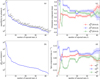 |
Fig. B.1 The evolution of loss and CRF link parameters with rejected star number k grows on the dataset 0 < G < 10.5. |
Appendix C Statistics of solution 0 < G < 10.5
Statistics of solution 0 < G < 10.5 for each star
Appendix D Radio star sky distribution
The sky distribution of the radio stars is shown in Fig. D.1. The whole sample lacks stars in the southern sky (< −30°). The number of stars between G = 9 and 13 is small and the stars are unevenly distributed, especially concentrated near the galactic plane, which may cause selection biases. A larger number of more evenly distributed available radio stars will help improve our results and reduce the impact of potential selection biases.
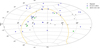 |
Fig. D.1 The sky distribution (Aitoff projection in equatorial coordinates) of the radio stars used in this study. The blue squares and green diamonds denote samples used in solution 0 < G < 10.5 and 10.5 < G < 13, respectively. The rejected stars are plotted as grey dots. The Galactic Equator is plotted in yellow. |
Appendix E Mathematics for orientation-only solution
The solution is based on Sect. 2 of Zhang et al. (2024), and the modifications needed for the orientation-only solution are as follows:
Proper motions of Gaia data μ = [μα*, μδ]′ need to be corrected with the a priori spin parameter ω = [ωX, ωY, ωZ]′ before the solution
 (E.1)
(E.1)
where
![Mathematical equation: $\boldsymbol{L}=\left[\begin{array}{ccc}\mathrm{c} \alpha_{i} \mathrm{~s} \delta_{i} & \mathrm{~s} \alpha_{i} \mathrm{~s} \delta_{i} & -\mathrm{c} \delta_{i} \\ -\mathrm{s} \alpha_{i} & \mathrm{c} \alpha_{i} & 0\end{array}\right];$](/articles/aa/full_html/2025/07/aa55160-25/aa55160-25-eq10.png) (E.2)
(E.2)
The parameters to be estimated is changed to x = [εX(T), εY(T), εZ(T)]′;
Because of the shape of x is changed from 6 × 1 to 3 × 1, the coefficient matrix Ki also needs to be changed to
![Mathematical equation: $\boldsymbol{K}_{i}=\left[\begin{array}{ccc}\mathrm{c} \alpha_{i} \mathrm{~s} \delta_{i} & \mathrm{~s} \alpha_{i} \mathrm{~s} \delta_{i} & -\mathrm{c} \delta_{i} \\ -\mathrm{s} \alpha_{i} & \mathrm{c} \alpha_{i} & 0 \\ 0 & 0 & 0 \\ 0 & 0 & 0 \\ 0 & 0 & 0\end{array}\right]$](/articles/aa/full_html/2025/07/aa55160-25/aa55160-25-eq11.png) (E.3)
(E.3)
to match the shape of x.
Appendix F Solution correlation coefficient matrices
Solution 0 < G < 13
![Mathematical equation: $\begin{align*}\operatorname{corr}\left[\varepsilon_{X}(T), \varepsilon_{Y}(T), \varepsilon_{Z}(T), \omega_{X}, \omega_{Y}, \omega_{Z}\right] & = \\ & \left[\begin{array}{cccccc} +1.000 & +0.191 & +0.204 & -0.102 & -0.120 & -0.206 \\ \ldots & +1.000 & +0.277 & -0.139 & -0.214 & -0.105 \\ \ldots & \ldots & +1.000 & -0.177 & -0.090 & -0.154 \\ \ldots & \ldots & \ldots & +1.000 & -0.032 & +0.099 \\ \ldots & \ldots & \ldots & \ldots & +1.000 & -0.021 \\ \ldots & \ldots & \ldots & \ldots & \ldots & +1.000\end{array}\right]\end{align*}$](/articles/aa/full_html/2025/07/aa55160-25/aa55160-25-eq12.png) (F.1)
(F.1)
Solution 0 < G < 10.5
![Mathematical equation: $\begin{align*} & \operatorname{corr}\left[\varepsilon_{X}(T), \varepsilon_{Y}(T), \varepsilon_{Z}(T), \omega_{X}, \omega_{Y}, \omega_{Z}\right] = \\ & \left[\begin{array}{cccccc} +1.000 & +0.134 & +0.192 & -0.166 & -0.100 & -0.237 \\ \ldots & +1.000 & +0.255 & -0.132 & -0.279 & -0.091 \\ \ldots & \ldots & +1.000 & -0.213 & -0.068 & -0.280 \\ \ldots & \ldots & \ldots & +1.000 & -0.043 & +0.120 \\ \ldots & \ldots & \ldots & \ldots & +1.000 & -0.043 \\ \ldots & \ldots & \ldots & \ldots & \ldots & +1.000 \end{array}\right] \end{align*}$](/articles/aa/full_html/2025/07/aa55160-25/aa55160-25-eq13.png) (F.2)
(F.2)
Orientation-only solution 0 < G < 13
![Mathematical equation: $\operatorname{corr}\left[\varepsilon_{X}(T), \varepsilon_{Y}(T), \varepsilon_{Z}(T)\right]=\left[\begin{array}{ccc}+1.000 & +0.142 & +0.158 \\ \cdots & +1.000 & +0.239 \\ \cdots & \cdots & +1.000\end{array}\right]$](/articles/aa/full_html/2025/07/aa55160-25/aa55160-25-eq14.png) (F.3)
(F.3)
Orientation-only solution 0 < G < 10.5
![Mathematical equation: $\operatorname{corr}\left[\varepsilon_{X}(T), \varepsilon_{Y}(T), \varepsilon_{Z}(T)\right]=\left[\begin{array}{ccc}+1.000 & +0.069 & +0.102 \\ \cdots & +1.000 & +0.206 \\ \cdots & \cdots & +1.000\end{array}\right]$](/articles/aa/full_html/2025/07/aa55160-25/aa55160-25-eq15.png) (F.4)
(F.4)
Orientation-only solution 10.5 < G < 13
![Mathematical equation: $\operatorname{corr}\left[\varepsilon_{X}(T), \varepsilon_{Y}(T), \varepsilon_{Z}(T)\right]=\left[\begin{array}{ccc}+1.000 & +0.414 & +0.345 \\ \cdots & +1.000 & +0.397 \\ \cdots & \cdots & +1.000\end{array}\right]$](/articles/aa/full_html/2025/07/aa55160-25/aa55160-25-eq16.png) (F.5)
(F.5)
References
- Asaki, Y., Deguchi, S., Imai, H., et al. 2010, ApJ, 721, 267 [NASA ADS] [CrossRef] [Google Scholar]
- Astropy Collaboration (Price-Whelan, A. M., et al.,) 2022, ApJ, 935, 167 [NASA ADS] [CrossRef] [Google Scholar]
- Bartel, N., Bietenholz, M. F., Lebach, D. E., et al. 2015, Class. Quant. Grav., 32, 224021 [NASA ADS] [CrossRef] [Google Scholar]
- Bobylev, V. V., 2022, Astron. Lett., 48, 790 [Google Scholar]
- Brandt, T. D., 2018, ApJS, 239, 31 [Google Scholar]
- Cantat-Gaudin, T., & Brandt, T. D., 2021, A&A, 649, A124 [NASA ADS] [CrossRef] [EDP Sciences] [Google Scholar]
- Charlot, P., 2025, in International VLBI Service for Geodesy and Astrometry 2024 General Meeting Proceedings, eds. D. Behrend, K. D. Baver, & K. L. Armstrong, 300 [Google Scholar]
- Charlot, P., Jacobs, C. S., Gordon, D., et al. 2020, A&A, 644, A159 [EDP Sciences] [Google Scholar]
- Chen, W., Zhang, B., Zhang, J., et al. 2023, MNRAS, 524, 5357 [Google Scholar]
- Ding, Y., Liao, S., Wu, Q., Qi, Z., & Tang, Z., 2024, A&A, 691, A81 [NASA ADS] [CrossRef] [EDP Sciences] [Google Scholar]
- Gaia Collaboration (Prusti, T., et al.,) 2016, A&A, 595, A1 [NASA ADS] [CrossRef] [EDP Sciences] [Google Scholar]
- Gaia Collaboration (Klioner, S. A., et al.,) 2022, A&A, 667, A148 [NASA ADS] [CrossRef] [EDP Sciences] [Google Scholar]
- Gaia Collaboration (Vallenari, A., et al.,) 2023, A&A, 674, A1 [NASA ADS] [CrossRef] [EDP Sciences] [Google Scholar]
- Galli, P. A. B., Loinard, L., Ortiz-Léon, G. N., et al. 2018, ApJ, 859, 33 [Google Scholar]
- Harris, C. R., Millman, K. J., van der Walt, S. J., et al. 2020, Nature, 585, 357 [NASA ADS] [CrossRef] [Google Scholar]
- Hunter, J. D., 2007, Comput. Sci. Eng., 9, 90 [NASA ADS] [CrossRef] [Google Scholar]
- Kounkel, M., Hartmann, L., Loinard, L., et al. 2017, ApJ, 834, 142 [Google Scholar]
- Kusuno, K., Asaki, Y., Imai, H., & Oyama, T., 2013, ApJ, 774, 107 [NASA ADS] [CrossRef] [Google Scholar]
- Lestrade, J. F., Preston, R. A., Jones, D. L., et al. 1999, A&A, 344, 1014 [NASA ADS] [Google Scholar]
- Lindegren, L., 2020, A&A, 633, A1 [Google Scholar]
- Lindegren, L., Hernández, J., Bombrun, A., et al. 2018, A&A, 616, A2 [NASA ADS] [CrossRef] [EDP Sciences] [Google Scholar]
- Lindegren, L., Bastian, U., Biermann, M., et al. 2021a, A&A, 649, A4 [NASA ADS] [CrossRef] [EDP Sciences] [Google Scholar]
- Lindegren, L., Klioner, S. A., Hernández, J., et al. 2021b, A&A, 649, A2 [NASA ADS] [CrossRef] [EDP Sciences] [Google Scholar]
- Loinard, L., Torres, R. M., Mioduszewski, A. J., et al. 2007, ApJ, 671, 546 [NASA ADS] [CrossRef] [Google Scholar]
- Lunz, S., Anderson, J. M., Xu, M. H., et al. 2023, A&A, 676, A11 [NASA ADS] [CrossRef] [EDP Sciences] [Google Scholar]
- Lunz, S., Anderson, J. M., Xu, M. H., et al. 2024, A&A, 689, A134 [NASA ADS] [CrossRef] [EDP Sciences] [Google Scholar]
- Malkin, Z., 2016, MNRAS, 461, 1937 [Google Scholar]
- Melis, C., Reid, M. J., Mioduszewski, A. J., Stauffer, J. R., & Bower, G. C., 2014, Science, 345, 1029 [NASA ADS] [CrossRef] [Google Scholar]
- Miller-Jones, J. C. A., Sivakoff, G. R., Knigge, C., et al. 2013, Science, 340, 950 [NASA ADS] [CrossRef] [Google Scholar]
- Nakagawa, A., Tsushima, M., Ando, K., et al. 2008, PASJ, 60, 1013 [NASA ADS] [Google Scholar]
- Nyu, D., Nakagawa, A., Matsui, M., et al. 2011, PASJ, 63, 63 [NASA ADS] [CrossRef] [Google Scholar]
- Ortiz-León, G. N., Dzib, S. A., Kounkel, M. A., et al. 2017a, ApJ, 834, 143 [Google Scholar]
- Ortiz-León, G. N., Loinard, L., Kounkel, M. A., et al. 2017b, ApJ, 834, 141 [Google Scholar]
- Peterson, W. M., Mutel, R. L., Lestrade, J. F., Güdel, M., & Goss, W. M., 2011, ApJ, 737, 104 [NASA ADS] [CrossRef] [Google Scholar]
- Reid, M. J., McClintock, J. E., Narayan, R., et al. 2011, ApJ, 742, 83 [Google Scholar]
- The pandas development Team 2024, https://doi.org/10.5281/zenodo.3509134 [Google Scholar]
- Torres, R. M., Loinard, L., Mioduszewski, A. J., & Rodríguez, L. F., 2007, ApJ, 671, 1813 [NASA ADS] [CrossRef] [Google Scholar]
- Torres, R. M., Loinard, L., Mioduszewski, A. J., et al. 2012, ApJ, 747, 18 [NASA ADS] [CrossRef] [Google Scholar]
- van Leeuwen, F., 2007, Hipparcos, the New Reduction of the Raw Data, 350 [Google Scholar]
- Vlemmings, W. H. T., & van Langevelde, H. J., 2007, A&A, 472, 547 [NASA ADS] [CrossRef] [EDP Sciences] [Google Scholar]
- Wenger, M., Ochsenbein, F., Egret, D., et al. 2000, A&AS, 143, 9 [NASA ADS] [CrossRef] [EDP Sciences] [Google Scholar]
- Zhang, J., 2025, https://doi.org/10.5281/zenodo.15031704 [Google Scholar]
- Zhang, B., Reid, M. J., Menten, K. M., & Zheng, X. W., 2012, ApJ, 744, 23 [NASA ADS] [CrossRef] [Google Scholar]
- Zhang, J., Zhang, B., Xu, S., et al. 2024, MNRAS, 529, 2062 [Google Scholar]
All Tables
All Figures
|
Fig. 1 Evolution of loss and rotation parameters with rejected star number, k, increasing in the full dataset (0 < G < 13). (a) Max Qi(x) in the solution (star names labeled). (b) |
| In the text | |
|
Fig. 2 Orientation-magnitude relationship of orientation-only solutions. Hollow markers denote the solution 0 < G < 13. Markers are horizontally shifted by 0.05 to avoid error bars overlapping. Horizontal lines of markers represent their magnitude range. |
| In the text | |
|
Fig. B.1 The evolution of loss and CRF link parameters with rejected star number k grows on the dataset 0 < G < 10.5. |
| In the text | |
|
Fig. D.1 The sky distribution (Aitoff projection in equatorial coordinates) of the radio stars used in this study. The blue squares and green diamonds denote samples used in solution 0 < G < 10.5 and 10.5 < G < 13, respectively. The rejected stars are plotted as grey dots. The Galactic Equator is plotted in yellow. |
| In the text | |
Current usage metrics show cumulative count of Article Views (full-text article views including HTML views, PDF and ePub downloads, according to the available data) and Abstracts Views on Vision4Press platform.
Data correspond to usage on the plateform after 2015. The current usage metrics is available 48-96 hours after online publication and is updated daily on week days.
Initial download of the metrics may take a while.