| Issue |
A&A
Volume 676, August 2023
|
|
|---|---|---|
| Article Number | A11 | |
| Number of page(s) | 23 | |
| Section | Celestial mechanics and astrometry | |
| DOI | https://doi.org/10.1051/0004-6361/202040266 | |
| Published online | 27 July 2023 | |
Enhancing the alignment of the optically bright Gaia reference frame with respect to the International Celestial Reference System
1
GFZ German Research Centre for Geosciences,
14473
Potsdam, Telegrafenberg, Germany
e-mail: This email address is being protected from spambots. You need JavaScript enabled to view it.
2
Technische Universität Berlin, Chair of Satellite Geodesy,
Kaiserin-Augusta-Allee 104-106,
10553
Berlin, Germany
3
Aalto University Metsähovi Radio Observatory,
Metsähovintie 114,
02540
Kylmälä, Finland
4
Aalto University Department of Electronics and Nanoengineering,
PL15500,
00076
Aalto, Finland
5
Geoscience Australia,
PO Box 378,
Canberra
2601, Australia
6
United States Naval Observatory (USNO),
3450 Massachusets Ave NW,
Washington, DC
20392, USA
Received:
31
December
2020
Accepted:
10
May
2023
Abstract
Context. The link of the Gaia frame in terms of non-rotation with respect to the International Celestial Reference System (ICRS), which is realized via very long baseline interferometry (VLBI) at radio wavelengths, has to be conducted for the wide range of optical magnitudes in which the spacecraft observes. There is a sufficient number of suitable counterparts between the two measurement systems for optically faint objects. However, the number of common optically bright (G ≤ 13 mag) objects is sparse as most are faint at radio frequencies, and only a few objects suitable for astrometry have been observed by VLBI in the past. As a result, rotation parameters for the optically bright Gaia reference frame are not yet determined with sufficient accuracy.
Aims. The verification of the Gaia bright frame of DR2 and EDR3 is enhanced by the reevaluation of existing VLBI observations and the addition of newly acquired data for a sample of optically bright radio stars.
Methods. Historical data from the literature were reevaluated, ensuring that the calibrator positions and uncertainties (used for the determination of the absolute star positions in the phase-referencing analysis) were updated and homogeneously referred to the ICRF3, the third realization of the International Celestial Reference Frame. We selected 46 suitable optically bright radio stars from the literature for new radio observations, out of which 32 were detected with the VLBA in continuum mode in the X or C band, along with radio-bright calibrators in the ICRF3. Improved Gaia-VLBI rotation parameters were obtained by adding new observations and utilizing more realistic estimates of the absolute position uncertainties for all phase-referenced radio observations.
Results. The homogenization greatly improved the steadiness of the results when the most discrepant stars were rejected one after another through a dedicated iterative process. For Gaia DR2, this homogenization reduced the magnitude of the orientation parameters to less than 0.5 mas but increased that of the spin parameters, with the largest component being the rotation around the Y axis. An adjustment of the position uncertainties improved the reliability of the orientation parameters and the goodness of fit for the iterative solutions. Introducing the new single-epoch positions to the analysis reduced the correlations between the rotation parameters. The final spin for Gaia DR2 as determined by VLBI observations of radio stars is (−0.056, −0.113, +0.033) ± (0.046, 0.058, 0.053) mas yr−1. A comparison of the new results with external, independently derived spin parameters for Gaia DR2 reveals smaller differences than when using the historical data from the literature. Applying the VLBI data to Gaia EDR3, which was already corrected for spin during Gaia processing, the derived residual spin is (+0.022, +0.065, −0.016) ± (0.024, 0.026, 0.024)mas yr−1, showing that the component in Y is significant at the 2.4σ level.
Conclusions. Even though our analysis provides a more accurate frame tie, more VLBI data are needed to refine the results and reduce the scatter between iterative solutions.
Key words: astrometry / reference systems / radio continuum: stars / methods: data analysis / methods: observational / instrumentation: interferometers
© The Authors 2023
 Open Access article, published by EDP Sciences, under the terms of the Creative Commons Attribution License (https://creativecommons.org/licenses/by/4.0), which permits unrestricted use, distribution, and reproduction in any medium, provided the original work is properly cited.
This article is published in open access under the Subscribe to Open model. This email address is being protected from spambots. You need JavaScript enabled to view it. to support open access publication.
1 Introduction
The Gaia spacecraft (Gaia Collaboration 2016b), operated by the European Space Agency (ESA) and launched in late 2013, has produced the most complete astrometric catalog of our Galaxy and the Local Group at optical wavelengths. In the first 22 months of its operations, it collected information about 1.7 billion objects, which was published as Data Release 2 (DR2; Gaia Collaboration 2018). Recently, the Gaia Early Data Release 3 (EDR3) was published, which is based on 34 months of observations and contains new astrometric data for about 1.8 billion sources (Gaia Collaboration 2021a). These data already outperform any other astronomical catalog and will very likely remain the most accurate source of optical positions for several decades into the future. Thus, verifying Gaia’s orientation and spin, particularly for the time after mission end when spin and proper motion errors dominate the position errors, is essential for high-precision navigation and orientation in space. This especially holds for optically bright objects, which are regularly used for attitude control and are being tested for use in deep space navigation beyond the medium Earth orbit (Martin-Mur et al. 2017, Optical Navigation Experiment1).
A suitable measurement technique for linking the Gaia catalog to the International Celestial Reference System (ICRS; Arias et al. 1995) is geodetic very long baseline interferometry (VLBI). This measurement technique is regularly utilized by observing extragalactic compact radio sources and creating a celestial reference frame by solving for global positions of the radio sources from observations spanning more than 40 yr. The resulting catalogs reach a similar accuracy as that of Gaia DR2. The latest official realization is the Third International Celestial Reference Frame (ICRF3; Charlot et al. 2020), which was derived from data at S/X frequencies between March 1979 and March 2018. It includes positions for 4 536 objects with a noise floor of 30 microarcseconds (μas). For the first time, two further catalogs were published together with the S/X catalog, which list VLBI positions of radio sources from observations at 22 GHz and 32 GHz. These catalogs were aligned to the S/X catalog. The three catalogs also consider the effect of the galactocentric acceleration of the Solar System, which shows up in the data as effects with a global dipole pattern of apparent proper motions toward the Galactic center with an amplitude of 5.8 μas yr−1 (MacMillan et al. 2019). The positions consequently have an epoch, namely 2015.0. An unpublished prototype of this catalog was used to orient the Gaia DR2 catalog to the ICRS (2017-06-30, solution from GSFC, IAU Working Group Third Realization of International Celestial Reference Frame), and the spin was aligned to the prototype ICRF and AllWISE (mid-infrared) active galactic nucleus catalogs (Secrest et al. 2015, 2016). The alignment is confirmed to within ±20 μas for orientation and ±20 μas yr−1 for spin per axis (Lindegren et al. 2018) for the optically faint part of DR2, with a magnitude range of G ≳ 15 and a median magnitude of G ≃ 18.8. The celestial reference frame of Gaia EDR3 was aligned toward ICRF3 within ± 10 μas in orientation at epoch 2016.0 and with a spin of less than ± 10 μas yr−1, both values at magnitude G =19 (Gaia Collaboration 2021a).
The calibration processing in Gaia is separated into an optically faint and an optically bright part (where G < 13 mag), and therefore the bright fraction of the data set needs to be verified as well. Since the extragalactic objects are mostly optically faint (for DR2, all are fainter than G = 13 mag and 99.9% are fainter than G =16 mag), the bright Gaia reference frame was examined with a different method. In Lindegren et al. (2018) the orientation of the bright fraction of DR2 is verified at a level of ±0.4 milliarcseconds (mas) per axis at epoch T = 2015.5 by using positions and proper motions of about 20 radio stars found in the literature. The spin of the bright fraction was determined from stellar proper motion differences between DR2 and the Tycho-Gaia astrometric solution (TGAS; Lindegren et al. 2016) in DR1 (Gaia Collaboration 2016a) for 88 091 objects in the HIPPARCOS (van Leeuwen 2007; ESA 1997) subset of the TGAS. A significant spin of ~0.15 mas yr−1 is found. It is a result of uncalibrated instrumental effects, which will be resolved in future Gaia data releases (Lindegren 2020a). However, the parameters still have to be verified. In future data releases, the comparison to the HIPPARCOS data set will no longer be sufficiently accurate (Lindegren 2020a). It is suggested that VLBI observations of optically bright radio stars can be utilized for the link in both orientation and spin instead. Accordingly, an algorithm was published by Lindegren (2020a,b) that uses positions, proper motions, and parallaxes of stars from VLBI and Gaia to derive the six rotation parameters. Three parameters each represent the orientation and spin about the three coordinate axes. In addition, radial velocities (needed for the rotation parameter adjustment) were taken from SIMBAD Astronomical Database (Wenger et al. 2000) whenever possible, as was done for 53 HIPPARCOS sources in DR2 (Lindegren et al. 2018). The setup also allows the inclusion of single positional measurements at one epoch or proper motion measurements without absolute positions. The algorithm was tested in Lindegren (2020a) on a sample of 41 stars found in the literature. However, only the 26 best-fitting stars were included in the final solution. The orientation offset is determined to be (ϵX, ϵY, ϵZ)=(−0.019,+1.304,+0.553)±(0.158,0.349,0.135) mas, thus revealing that the offsets around the Y and Z axes are significant. The high uncertainty for the Y component results from the nonoptimal spatial distribution of the more recent VLBI observations. The spin of the DR2 bright fraction is determined to be (ωX, ωY, ωZ)=(−0.068,−0.051,−0.014)±(0.052,0.045, 0.066) mas yr−1 relative to the VLBI reference frame (Lindegren 2020b) and is thus not significant. Similar results for the spin parameters are independently obtained by Brandt (2018).
These results are not as accurate as desired, given that the expected uncertainties for bright objects with G ≤ 13 mag in the final Gaia data release will be less than 7.7 μas for positions and 5.4 μas yr−1 for proper motions according to de Bruijne et al. (2014). First, the major limitation of using VLBI observations of radio stars is their sparseness both in time and sky distribution. Second, many stars are located in multi-star systems, which requires the modeling of nonlinear motions. Third, binaries with separations of less than 100 mas are not resolved by Gaia and results refer to the photocenter (Lindegren et al. 2018), whereas they are resolved by VLBI and multiple components are detected. Fourth, radio-optical offsets of the observed emission of the stars should be considered, as the radio emission might not stem from the same position as the optical emission (Andrei et al. 1995). Because of these limitations, more radio observations of suitable optically bright stars are needed to reach the desired level of accuracy for a successful verification (Lindegren 2020a).
Most suitable stars are faint at radio frequencies, and only a few can be directly measured in absolute astrometry mode by VLBI as done for extragalactic objects in the ICRF (Titov et al. 2020). For this reason, phase-referencing as a relative observing method is commonly used for those faint targets (Wrobel et al. 2000). In this technique, a bright primary calibrator is alternately observed with the weak target. The phases from which source positions are derived can thus be determined for the bright object with a good signal-to-noise ratio (S/N) and transferred to the weak object. Thereby, precise positions of the weak objects can be determined relative to the bright objects (Reid & Honma 2014). If source positions from ICRF3 are used for the calibrators, the derived positions of the radio-weak targets are also those of the ICRF3. Furthermore, if the calibrator position improves in the future (e.g., through another realization of the ICRF), the position of the target will also improve.
This paper reports on the homogenization of data from the existing analysis of Lindegren (2020a). This homogenization was carried out by referencing the model positions of the stars to a common reference frame, obtaining a realistic error budget estimation for absolute positions from phase-referencing, and using new observations of stars in radio frequencies to enhance the verification of the Gaia bright reference frame. For the new observations, we selected 46 known radio stars from the literature and conducted a survey with the Very Long Baseline Array (VLBA) to see which of them would be suitable for further astrometric measurements. The original purpose of the observations was to determine the peak intensities of the stars and calibrators in order to adjust on-source time for a high S/N in subsequent observations. While we report such peak intensities in the following, we also make use of the star positions derived from this short experiment to enhance the estimates of rotation parameters between the Gaia and ICRF3 S/X frames in various test scenarios.
Section 2 describes the effort to homogenize the historical data and gives information about the observational setup, processing, and results of the new observations. The star position differences from phase-referencing to multiple calibrators as well as the position differences between the barycenter and the center of luminosity for unresolved binaries as seen by Gaia are examined. In Sect. 3 the mathematical tools for the fit of the rotation parameters and the evaluation of the iterative results are given. Realistic uncertainty estimates for the absolute positions of stars from phase-referencing are also derived. In Sect. 4 various rotation parameter solutions are shown using Gaia DR2 and Gaia EDR3 data. In Sect. 5 we discuss the results, and Sect. 6 provides conclusions and an outlook. In the following, the abbreviation α* = α · cos(δ) for the right ascension coordinate and a similar one for its uncertainty are used.
2 Processing of historical and new VLBI data
Lindegren (2020a) provides a determination of rotation parameters between the Gaia bright frame and the ICRF3 based on the collection of radio star positions, proper motions, and parallaxes provided in his Table 1. We evaluated the list and extended it with star positions from dedicated observations in January 2020. Using the Gaia identifier in Table 1 below, the respective Gaia data can be obtained from the Gaia archive directly, and therefore the data are not presented here.
2.1 Homogenization of historical data
As a first step, we evaluated the data in Table 1 of Lindegren (2020a). As mentioned by Lindegren (2020a), not all listed calibrator (and thus star) positions were transferred to ICRF3, some being left in the original frame. As this could result in a bias in the rotation parameters, we made efforts to transfer all such positions to ICRF3. Furthermore, it was found that the uncertainties of the star positions that were not transferred to ICRF3 did not take into account the uncertainties of the calibrator positions.
Not all original publications clearly indicate the calibrator positions used. If not found in the publication or in a cited catalog, the positions from .vex files or, if missing, from the .crd files in the VLBA observing archive2 were collected in order to obtain the calibrator positions most likely used. For some publications only the observed fields were given, but it was possible to connect each star to a field and then to identify the calibrator used by cross-referencing some of the tables in the respective publications. Thus, some assumptions were made, and crosschecks with the VLBA observation archive, where metadata of the observation sessions are stored, were performed. We assume that if the calibrator positions would have been changed after the scheduling or .vex file creation, it would have been mentioned in the respective publication. For one publication contradictory information was sorted out with the help of the main author. In all cases, the calibrator positions were given with a sufficient level of accuracy.
All original calibrator positions were identified and the differences to the ICRF3 positions were determined. They are listed in Table E.1. With this information, all star positions could be transformed to ICRF3 by applying the shifts Δα and Δδ between the original calibrator position αoriginal and δoriginal and the ICRF3 S/X catalog position. The ICRF3 catalog position uncertainties were applied as calibrator position uncertainties σα,CRF or σδ,CRF to the star position uncertainties. All star positions thereby have a consistent error budget. For S Per, the calibrator position and uncertainty from the rfc_2018b catalog (Petrov 2018) were taken, as the calibrator used is not present in ICRF3. It is indicated in Table E.1. As shown in Lunz et al. (2019), the rfc_2018b and ICRF3 S/X are aligned within about 50 Mas in orientation, which is acceptable at the current stage of analysis, considering the error level involved (see below). It is assumed that for the stars from references 3, 5, 14, and 17 in Table 1 of Lindegren (2020a) the model positions were already transformed to ICRF3, and the calibrator uncertainties from ICRF3 were applied, as stated in the publication. Furthermore, the two data entries for the star HD 283572 are based upon the same observational data but different calibration strategies (Galli et al. 2018); therefore, they are highly correlated3.
2.2 New one-epoch observations, data analysis, and results
In order to obtain a high probability of successful detections, it was decided to prioritize the re-observation of already known radio stars rather than testing continuum observations at radio frequencies of stars that have not yet been observed by VLBI on intercontinental baselines. This will also make it possible to refine the proper motions and parallaxes for stars within a short time by combining the data already available in the archive.
In Lunz et al. (2020) we made a literature search for stars that have been observed in radio continuum in the past and which are probably suitable for the radio-optical link. Further information on the selection process of stars and calibrators as well as the observation planning can be found in Appendix A. Both the primary calibrators, P 1, and the secondary calibrators, S 1 and S 2, were selected, with preference given to calibrators already employed in previous observations from the literature. If in previous observations of a star different primary calibrators were used regularly, two primary calibrators P 1 and P 2 were chosen to see if one of them was more suitable for current observations. The secondary calibrators were not used for any corrections of the star positions in this work but only for the determination of their peak intensities for better planning of follow-up observations. The sets of stars, calibrators, and the references can be found in Table 1. To be able to connect to phase-referencing results of historical data, the stars were observed at the same frequency bands (X or C band) that were employed in previous observations.
The project was split into three experiments as shown in Table E.2, so that it was possible to observe the stars within only 14h of VLBA observing time of the United States Naval Observatory (USNO) time-share agreement, while still getting a sufficient uv-coverage. The schedule for each star consisted of three blocks, where in each block the antennas observed the primary calibrator for 30 s, the target star for 100 s, and again the primary calibrator for 30 s. The time intervals were chosen to not lose phase-coherence between the scans of the primary calibrator at the given frequencies and considering the targetcalibrator separations (Marti-Vidal et al. 2010, 2011). The three observing blocks for each star were distributed over one or two of the three experiments as listed for each star in Table 1. In one of the blocks, the secondary calibrators were observed with one 30 s scan between the respective target and primary calibrator scans. Within an experiment, frequency setups were depending on the observed star. The center frequencies were 8.11225 GHz for observations in the X band and 4.61175 GHz for the C band. Four subbands with a bandwidth of 128 MHz each were used. Dual-polarization observations were recorded with a total data rate of 4 Gbit s−1. With this setup, stars as faint as 1 mJy beam−1 can be detected. For each experiment additional observations to a known bright compact source were scheduled, which are needed for instrumental calibrations like bandpass calibration and global fringe fitting. Two geodetic blocks of 30 min length each containing observations to bright radio sources at various elevations were included in each experiment at the end of the first third and the second third of the scheduled time slot, to allow for atmospheric corrections using group-delays according to Mioduszewski (2009). The data were correlated at the VLBA correlator in Socorro, New Mexico (USA).
The data were processed using the NRAO Astronomical Image Processing System (AIPS; Greisen 2003) as outlined in the AIPS cookbook4 and with the help of ParselTongue (Kettenis et al. 2006). In the X band, strong radio frequency interference (RFI) occurred at the Pie Town antenna, and in addition the observations collected by the antenna had very low S/N. We obtained better results after flagging the antenna entirely. In the C band, RFI occurred at the Brewster antenna and the respective subband (IF 1 at 4.6118 GHz in AIPS) was flagged.
The amplitude calibration was based on Walker (2014). The a priori Earth Orientation Parameters were corrected using the final series from the USNO. Then the dispersive delay from the ionosphere was removed utilizing global maps of total electron content derived from GPS observables and provided by the Jet Propulsion Laboratory (JPL). After the purely geometric parallactic angle correction was applied, the digital sampling correction to amplitudes was carried out. In the next step, instrumental delays and phases were corrected. Pulse-calibration information was used except for antennas with ambiguities in those data. For those antennas the corrections were done manually using the known bright compact radio source J0359+5057 in experiment UL005A, J0927+3902 in experiment UL005B, J2253+1608 in experiment UL005C in the X band, and J1927+7358 in experiment UL005C in the C band. Bandpass calibration was then performed, auto-correlations were calibrated to be unity, and a priori amplitude calibration was applied using system temperature and gain curve tables. Atmospheric opacity correction was negligible at the given frequencies. Multiband delays for the observations of the geodetic blocks were produced and used to correct for elevationand time-dependent delay errors for each antenna, as described in Mioduszewski (2009), by interpolation over all scans. The secondary calibrators are in principle used to calculate residual phase gradients between the primary calibrator and the secondary calibrator. With this additional information, the correction of the target positions can be improved using the task ATMCA in AIPS (Fomalont & Kogan 2005). However, it was not possible to employ this feature for our observations since the secondary calibrators were only scheduled in one of the three phase-referencing blocks in order to obtain their peak intensities for follow-on observations, as noted above.
A final fringe fit of each phase-referencing calibrator was made, and corrections were applied to the respective calibrator itself as well as to its associated secondary calibrators and target star. If an object was observed in multiple experiments, its data were combined after the instrumental calibrations. In all fringe fits the calibrators were assumed to be point sources, as was done in the geodetic VLBI analysis conducted for the creation of the ICRF3. If a star was observed by using two phase-referencing calibrators, the fringe fit of the calibrator data and subsequent steps were repeated for each of the calibrators.
From these data, CLEANed images (Högbom 1974; Clark 1980) with a cell size of 0.2 mas and natural weighting (robust =5) were produced in AIPS from which positions were derived using the task JMFIT. This task fits two-dimensional Gaussians to a given area including the source in the image. The position uncertainty resulting from this task is based on the expected theoretical precision of the interferometer and the RMS noise of the image.
An independent comparison was done with the MODELFIT task in the Caltech DIFMAP imaging package (Shepherd 1997)5. This task determines Gaussian model parameters of the radio source from the visibility data directly instead of from the image. The model can consist of multiple components. The uncertainty σrandom of a model component position was calculated from the beam shape and RMS noise of the image based on formulas for elliptical Gaussians in Condon (1997).
The evaluation of the differences in position of a star derived with both MODELFIT in DIFMAP and JMFIT in AIPS improved the reliability in the detection of faint stars and provided additional insights into the absolute position uncertainties from VLBI observations at individual epochs. We detected 32 out of the 46 observed stars with a dynamic range6 of 5 or higher. Details on the calculation of the peak intensities are given in Appendix B. Peak intensities for the 32 detected stars and calibrators are listed in Table B.1. The stars that could not be detected were HD 283641, V1961 Ori, HD 290862, RCMa, XYUMa, RVLib, AGDra, WWDra, HD 226868, ER Vul, RTLac, lamAnd, ZHer, and TYPyx. Three of the stars (HD 283447, DoAr51, and UXAri) are close binaries, and the identification of their individual Aa and Ab components is described in Appendix C.
We find that MODELFIT can be more robust to find the position of the centroid of emission if structure or multiple close components are present, which is why its results are used in the following analysis. Star coordinates are listed in Table E.3 as a(t) and δ(t) along with their uncertainties σα*,randam and σδ,randam. The epochs of observation t are displayed with five digits after the decimal point of the Julian year to represent 6 min time difference. This higher precision compared to information in other publications such as Lindegren (2020a) is needed, because star HD 224085 in our list has a proper motion of approximately 577 mas yr−1 according to literature. Such a proper motion translates to a position error of about 0.007 mas over the quoted 6-min time accuracy, which is acceptable. The three scans of this star were conducted within a time interval of 23 min in order to prevent significant smearing effects. The positions determined from the analysis of the single epoch observations were corrected for the influence of parallax to obtain positions referenced to the solar system barycenter that are comparable to those in the Gaia data releases. In addition, the influence of the Römer delay (geometrical delay associated with the observer’s motion around the Solar System barycenter) was corrected in order to obtain the barycentric time of light arrival, as explained in Appendix A of Lindegren (2020a). For these reductions we derived the barycentric coordinates of the Earth center at the time of observation from the DE 421 ephemeris (Folkner et al. 2009) using the VieVS@GFZ VLBI software developed by the German Research Centre for Geosciences (GFZ). For the investigation of the Gaia DR2 data set, the Gaia parallax was applied to all stars, as the VLBI parallax is not available for all objects (for example, for the stars in Boboltz et al. 2007), and a unified result was aimed for. The parallaxes of Gaia DR2 are known to be biased by a few tens of μas (Arenou et al. 2018). For faint quasars an offset of −0.03 mas was determined by Lindegren et al. (2018), but for brighter objects this parameter was determined to be larger. A variety of studies examining this topic by using different sets of stars and methods already exist (Riess et al. 2018; Schönrich et al. 2019; Zinn et al. 2019). Following Lindegren (2020a), a parallax offset of -0.05 mas was used to keep results comparable. In the last columns of Table E.3, the calculated Römer delay Roe (t) and the shifts to mitigate the parallax effect Δα (t) and Δδ (t) at the epoch of observation t, both using the Gaia DR2 parallax, are listed along with the radial velocity vr from SIMBAD, which is needed for the transformation of the Gaia results to the VLBI epoch in the rotation parameter adjustment (see below). For Gaia EDR3, the parallax correction is not static and a python implementation calculating the bias function provided in Lindegren et al. (2021a) was used instead. Corrections Δα (t) and Δδ (t) in Table E.3 are thus slightly different for Gaia DR2 and Gaia EDR3.
By using the method of phase-referencing to calibrator positions in the ICRF3, the resulting positions of the stars refer to the ICRF3. For those calibrators that are not part of ICRF3, positions from catalog rfc_2018b were used. This should not introduce position inconsistencies since the rfc_2018b catalog is reasonably well aligned with the ICRF3, as noted above. In this work, the effect of galactocentric acceleration on the calibrator positions in ICRF3, and thus on the star positions and proper motions, was ignored. This effect would show up as a tiny but systematic global dipole pattern (with an amplitude of about 5 μas yr−1) in the proper motions of the stars and it would be pointing toward the Galactic center (Titov et al. 2011; Xu et al. 2012; Titov & Krásná 2018; MacMillan et al. 2019). Only with Gaia EDR3 the Gaia internal systematics are small enough to detect this effect (Gaia Collaboration 2021b). At the current level of accuracy (see below), this effect was considered negligible and was not accounted for. An investigation of its impact is deferred to a later publication.
Calibrators, observation setup, and metadata for the 46 radio stars observed with the VLBA.
2.3 Multiple phase-referencing calibrators
Seven of the detected target stars, UX Ari, HD 283447, CoKu HP Tau G2, BHCVn, del Lib, ARLac, and SZPsc, were observed along with two different primary calibrators within the same respective observing block as indicated in Table 1. The pattern was P 1-P 2-star-P 1-P 2. Therefore, the star positions relative to P 1 and P 2 are highly correlated in terms of error sources like earth orientation, atmosphere, and uv-coverage; however both are valid results considering an appropriate error budget. This observational setup provides the opportunity to study the accuracy of the absolute positions of these stars. The positions derived with MODELFIT in DIFMAP were obtained from the same data set once with phase referencing all objects of the group, consisting of the star and the associated calibrators, to the primary calibrator P 1 and once with phase referencing all objects of the group to P 2. The results are also reported in Table E.3. The differences between the positional fits to P 1 and P 2, Δα* and Δδ, are presented in Table 2. These quantities can be used to quantify potential systematic errors in the absolute star positions, which is further investigated in Sect. 3.2.
The RMS of the offsets Δα* and Δδ is 0.47 mas in α* and 1.08 mas in δ. For comparison, the RMS of the standard deviations of the catalog positions of the calibrators σΔα*,CRF and σΔδ,CRF is 0.26 mas and 0.47 mas, respectively, which is a factor of 2 smaller than the RMS of the offsets. The RMS of the offsets in the α direction is half that in the δ direction. This could be due to the poor uv-coverage of our observations in the δ direction due to network geometry, as indicated by the beam sizes, and the short observation time span for most objects. For double stars only one component was considered for these calculations in order not to bias the results. For both UX Ari and del Lib, one of the calibrators is not part of the ICRF3, and thus its position and uncertainty were taken from the rfc_2018b catalog. However, the offsets for these two stars are not significantly different than those for the other stars and there seems to be no impact at the current level of precision. The offsets of the respective other primary and secondary calibrators observed along with the stars, as listed in Table 1, do not differ significantly from those of the stars.
The calibrator position from phase-referencing experiments best matches the ICRF3 catalog position if the radio source is compact. Xu et al. (2019a) examined 3417 celestial reference frame radio sources in terms of source structure effects in closure phase and amplitude signals over their whole observation history. They introduce the closure amplitude root mean square (CARMS). This quantity represents the lower boundary of structure effects that can be detected in the data. A CARMS value above 0.3 indicates a radio source with significant structure.
The CARMS values of Xu et al. (2019a) based on basic-noise weighting are used to verify the compactness of the primary calibrators. The values for our calibrators were confirmed by the closure statistics computed from the phase-referencing data itself. The calibrators chosen in the older historical observations, P 2 (except for del Lib, where both calibrators P 1 and P 2 are new), are usually very bright but have significant structure, whereas the other calibrators, P 1, were chosen because they are more compact. However, the latter are farther away in most cases. More work has to be conducted in order to better understand which calibrator should be chosen for future observations. Surely the decision will also depend on the availability and data quality of the single epoch data from the literature and the archive.
Difference Δα* and Δδ in the absolute positions of seven stars when phase-referenced to two different primary calibrators.
2.4 Unresolved binaries as seen by Gaia
As mentioned in Sect. 1, Gaia can only distinguish between objects more than 100 mas apart and otherwise will refer to the photocenter. In our data set three close binaries that were resolved by the VLBI observations are within this threshold at the time of observation and therefore unresolved by the Gaia spacecraft.
The barycenter of the stellar system can be chosen as a stable reference point for comparing the trajectory of the binary from VLBI and Gaia. It might however not be the same position as the photocenter of Gaia detections. Therefore, as an alternative, we also determined the center of luminosity, as we expect it to be closer to the photocenter observed by Gaia than the barycenter. Even if the binaries are located within a multiple star system, we apply the binary star model as an approximation as we detected only the emission of two components.
For HD 283447 the apparent separation between the two components of the binary system was determined to be (2.824 ± 0.070) mas in α* and (1.975 ± 0.174) mas in δ, which is the mean value of the observations to the first and the second primary calibrators (Fig. C.1). Respective values for DoAr 51 are (−4.031 ± 0.105) mas in α* and (−5.626 ± 0.309) mas in δ (Fig. C.2). The positions of the two best fitting Gaussian components for UX Ari differ on average by (−1.514 ± 0.030) mas in α* and (−0.268 ± 0.076) mas in δ (Fig. C.3).
For calculation of the barycenter coordinates of a binary system, the masses of the two components, m1 for the primary and m2 for the secondary, are needed. For HD 283447 Aa and Ab the masses are given in Torres et al. (2012), for DoAr 51 they are given in Ortiz-Leon et al. (2017b) and for UX Ari they are given in Hummel et al. (2017). Then, the vector r1 between the primary star position and the barycenter is (Torres et al. 2012) (1)
(1)
where r is the separation between the primary and secondary star.
The center of luminosity was calculated in the same manner, but instead of the masses the luminosities of the stars were used for the calculations. For HD 283447 the optical luminosities for components Aa and Ab are given in Welty (1995) and for UX Ari, they are given in Hummel et al. (2017). For DoAr 51 we determined a factor equivalent to  from the flux ratio in Schaefer et al. (2018), assuming that both stars are equally distant, since we could not find the luminosities directly. We used the J-band flux ratio because it is the closest to the Gaia bands. The components in α and δ of the vector r1, which provides the barycenter offset or luminosity center offset from the primary star and their differences, are listed in Table 3. They are several hundreds of microarcseconds large. These offsets can be added to the position of the primary star of the binary system to obtain the absolute positions of the barycenter and center of luminosity.
The differences between the barycenter and center of luminosity positions remain similar whether using the P 1 or the P 2 calibrator for phase-referencing. No clear sign could be found which of the two centers match better the Gaia position at the VLBI epoch. Therefore, no final conclusion can be made at this point, and the center of luminosity is used in the following.
3 Analysis method
In this section the relevant tools for the rotation parameter analysis and evaluation are described.
3.1 Combined fit of rotation parameters and corrections to the Gaia astrometric models
As we apply the same algorithm as introduced in Lindegren (2020a) for simultaneously fitting the orientation and spin parameters between VLBI and Gaia along with adjustments to the star model of Gaia transformed to the VLBI epoch, we only give a short description here. We use the same terms of “orientation”, denoted ϵ(T) = (ϵX(T), ϵY(T), ϵZ(T)) for conciseness, for the instantaneous global solid-body rotation between two reference frames about their three axes X, Y, and Z at reference epoch T, and of “spin,” denoted ω = (ωX, ωY, ωZ), for the corresponding the rotation rate. Consequently, an orientation offset at epoch t can be calculated as
 (2)
(2)
The coordinate differences from the orientation offset between two reference frames, in this case determined by VLBI and Gaia, are given by
 (3)
(3)
 (4)
(4)
where the star positions determined by VLBI, αVLBI and δVLBI, and the star positions determined by Gaia, αGaia and δGaia, are at the same epoch t. Similar equations are used for the differences in proper motion,
 (5)
(5)
 (6)
(6)
In the combined estimation of ϵ(T) and ω, written as the column vector x = [ϵX(T), ϵY(T), ϵZ(T), ωY, ωZ]’, the observables are the position, proper motion, and parallax differences, Δfi. These quantities are determined as the differences between the observed VLBI data and the Gaia data set propagated to the VLBI epoch, and are available for a total of S stars. The position offsets contribute to the determination of both orientation and spin, whereas the proper motion differences contribute to the spin determination only. The results of the least squares fit are an estimate  for the six rotation parameters between the two frames along with estimates of the five astrometric parameters for each star i (where i = 1…S), and their full covariance matrix. The residuals vi for the star i are calculated as the differences between the VLBI data and the predicted Gaia data corrected for the rotation offset using the estimates of the rotation parameters (for more information see Lindegren 2020a). The term
  describes the discrepancy of a star, i, for a given solution,
  , where ni is the number of observables for the star contained in the solution (i.e., the length of the vector Δfi). The quantity
  can be determined from the residuals vi as
 (7)
(7)
where Di is the covariance of Δfi. If the data fits the five-parameter astrometric model well and the uncertainties of the observables are correctly estimated, Qi/ni should be close to unity. We used this measure for the iterative analysis of the rotation parameters in the following way: after a first fit using all stars, the star with max(Qi/ni) is discarded from the data set and another fit involving only the new subset of stars is determined, then the star with max(Qi/ni) from the new fit is discarded as well, and so on. In the end, all possible solutions with k = 0,1,2,… discarded stars are analyzed. In addition, the quantity Q/n = Σ Qi/Σni, is used to evaluate the improvement of the overall fit at each iteration.
Components in α and δ of the vector r1, which provides the position of the barycenter or center of luminosity with respect to the position of the primary star for the close binary systems in UX Ari, HD 283447, and DoAr51.
3.2 Discussion on VLBI position error bounds
The positions derived in the previous sections are of two kinds, that is, the model positions from Sect. 2.1 and the single-epoch positions from Sect. 2.2. The single-epoch positions describe the star positions at a specific epoch in time. For these positions no averaging or correction for nonvisible binary companions and other disturbances could be applied. In contrast, the model positions from a fit of relative position time series to models of stellar motion (usually mean position, proper motion, and parallax) are affected by such disturbances. These would increase the uncertainty of the estimated astrometric parameters because the formal errors are usually adjusted so that the reduced χ2 of the fit equals unity. The impact is minimized by selecting stars with a small renormalized unit weight error (RUWE) parameter (calculated from Gaia DR2 data; Lindegren et al. 2018), indicating that the Gaia data fits the five-parameter astrometric model well, and by the iterative approach, where deviating stars get rejected first. Nevertheless, the difference of the error budget for the two types of positions needs further investigation, which is given in the following.
In general, positions derived from phase-referencing measurements, as in the present study, are affected by the following five thermal or systematic errors. The first is the random error σrandom [thermal] due to thermal noise calculated based on the S/N and the shape of the elliptical Gaussian fitted to the central map component (e.g., Thompson et al. 1986; Condon 1997). Mean (Median) values of 0.034(0.026) mas in α* and 0.087 (0.067) mas in δ are obtained from the data of this study.
The second is the celestial reference frame calibrator position uncertainty, σCRF [thermal]. The median position uncertainty in ICRF3 S/X is 0.1 mas in α and 0.2 mas in δ. The additional error due to the absolute position wander of individual calibrators, for example quantified by the Allan variance in Gattano et al. (2018), is ignored.
The third is the delay model error σdelay model [systematic] from residual ionospheric and tropospheric errors, antenna and calibrator position errors, and Earth orientation parameter errors. These mostly depend on the declination of the source and the calibrator-target separation. Pradel et al. (2006) determined that the combined error is roughly between 0.015 mas to 0.284 mas per coordinate direction for a calibrator-target separation of 1° based on a simulation without ionospheric delay uncertainty considered. The uncertainty due to residual ionospheric delay from JPL total electron content maps is below 0.1 mas.
The fourth is the source structure error σstructure [systematic] due to non-point-like and possibly varying calibrator structure. The larger the structure, the higher the effect. When modeling calibrator structure, the positions of the stars estimated in our analysis show a mean difference of −0.003 mas in α* and 0.002 mas in δ, while the RMS of the differences is 0.019 mas in α* and 0.035 mas in δ.
The last is the uncertainty σphase-group [systematic] due to the difference between calibrator groupand phase-delay positions in the presence of core shift (possibly varying with time). This uncertainty was determined to be between 0.036 mas and 0.326 mas for a source with a median core shift between the S and X band of 0.44 mas (Kovalev et al. 2008) and for a variety of power-law exponents (Porcas 2009). We anticipate the impact of core shift in the C band to be smaller since this frequency lies between the S and X frequency bands. In practice, it is possible that σphase-group is also affected by structure at S band, which impacts the S/X positions, but this is only a second order effect.
All of these effects are unique in magnitude and direction in the sky from radio sources to radio sources.
A possible way to get insights into the magnitude of unaccounted systematic errors in the single-epoch positions may be obtained by comparing absolute star positions determined by phase-referencing with respect to two different calibrators (see Sect. 2.3). In principle, that is to say, in the absence of systematic errors, the difference in the absolute positions of a star measured in such a case should be consistent with the uncertainties derived from a combination of the positions uncertainties of the two calibrators in the ICRF3, σΔα*,CRF and σΔδ,CRF. Any difference larger than that reveals the presence of systematic errors. In our analysis (see Sect. 2.3 and Table 2), the RMS of the differences of the star positions, Δα* and Δδ, is on average twice as large as the combined calibrator uncertainties, σΔα*,CRF and σΔδ,CRF. Thus, our analysis is not free of systematic errors. To evaluate the magnitude of such systematic errors, we subtracted in quadrature the RMS of σΔα*,CRF and σΔδ,CRF, respectively, from the RMS of Δα* and Δδ, as  mas for α* and
  mas for δ. The errors thus determined can then be added to the thermal errors σrandom and σCRF to get the absolute star position uncertainties, expressed as
![Mathematical equation: $\sigma _{\alpha * ,{\rm{absolute}}}^{{\rm{single}}\,{\rm{epoch}}} = \sqrt {\sigma _{\alpha * ,{\rm{random}}}^2 + {{\left[ {{\sigma _{\alpha ,{\rm{CRF}}}} \cdot \cos \left( \delta \right)} \right]}^2} + {{0.25}^2}} {\rm{mas}}$](/articles/aa/full_html/2023/08/aa40266-20/aa40266-20-eq17.png) (8)
(8)
and
 (9)
(9)
The values of these absolute positional uncertainties are reported in Table 4 for each of the 32 detected individual stars in addition to their random errors. The mean (median) of such values for all stars in our sample are 0.315 (0.305) mas for α* and 0.738 (0.714) mas for δ.
In case of star positions derived from fitting models of stellar motion to multi-epoch relative positions, many systematic errors were accounted for by inflating the formal errors such that the χ2 of the fit equals one. Such inflated errors are labeled σmodelpos; if the σCRF were added (as it was done for the homogenization efforts in Sect. 2.1). However, not all systematic errors can be accounted for by this method. To complete the error budget, an additional component to account for σphase-group still needs to be applied. We found three approaches for estimating the magnitude of this uncertainty. First, the difference between group-delay position and phase-delay position determined from simulations in Porcas (2009) is 0.166 mas for a core shift of 0.440 mas between 2.3 GHz and 8.4 GHz, and in the case of an ideal source having no jet. Second, Fomalont et al. (2011) studied the difference between ICRF2 positions and positions from phase-referencing at 8.6 GHz for four compact radio sources by using the VLBA. The conclusion was that the positions in ICRF2 can be offset from the phase-referenced positions (materialized by the core of the sources) by up to 0.5 mas, with the mean offset being 0.42mas. Dividing this value by  a σphase-group magnitude of 0.30 mas per coordinate direction is obtained. Third, the trajectory of the Cassini spacecraft was observed at 8.4 GHz relative to various primary calibrators by the VLBA as well (Jones et al. 2020). From this study, σphase-group was determined to be in the range of 0.18 mas to 0.20 mas, similar to the above values. The mean value of the three approaches is 0.21 mas. For star positions observed in the C band, the magnitude might be smaller due to the C band being in between the S- and X-band frequencies. However, this is not considered in this study. Based on our analysis, an extra noise of 0.21 mas was thus added to σmodel pos to obtain a more realistic error budget for the absolute positions derived from models of stellar motions:
 (10)
(10)
and
 (11)
(11)
The more realistic error budget for the absolute positions presented in this section must be used when comparing the two kinds of absolute positions from VLBI (single-epoch or derived from models of stellar motions) to an independent measurement system such as Gaia.
3.3 Metrics for evaluating the rotation parameters
To compare the iterative solutions of the rotation parameters for various scenarios s, the steadiness of the parameters can be used as a criterion for the reliability of such solutions. Three quantities were computed to this end: (i) the weighted mean (WM) of the rotation parameters, WMs, (ii) the weighted root mean square (WRMS) of the difference between the rotation parameters at each iteration and the WM over all iterations, WRMSs, and (iii) the mean of the parameter formal errors, MEs. These quantities can be expressed as
 (12)
(12)
![Mathematical equation: $WRM{S_s} = \sqrt {{{\left( {j i + 1} \right)\sum\nolimits_{k = i}^j {\left[ {{{\left( {{{\hat x}_k} {\rm{W}}{{\rm{M}}_{\rm{s}}}} \right)}^2}\left( {{1 \mathord{\left/ {\vphantom {1 {\sigma _k^2}}} \right. \kern-\nulldelimiterspace} {\sigma _k^2}}} \right)} \right]} } \over {\left( {j i} \right)\sum\nolimits_{k = i}^j {{1 \mathord{\left/ {\vphantom {1 {\sigma _k^2}}} \right. \kern-\nulldelimiterspace} {\sigma _k^2}}} }},} $](/articles/aa/full_html/2023/08/aa40266-20/aa40266-20-eq23.png) (13)
(13)
 (14)
(14)
where  is the rotation parameter of interest at iteration k and σk its uncertainty. Only a representative range of iterations was used to derive these quantities. The start, i, of the selected iterations was chosen so that no outliers were included, and the stop, j, was chosen to avoid having too few stars left in the sample and thereby allow us to obtain reliable estimates of the rotation parameters. For solutions without the January 2020 positions, the WMs and WRMSs were calculated from iterations i = 9 to j = 34, while for solutions including the January 2020 positions, iterations i = 12 to j = 47 were considered. When calculating MEs, the last ten iterations were left out because the formal errors then tend to be larger compared to those in the range of iterations where the baseline solution is normally chosen.
If WRMSs is two times larger than MEs, the rotation parameter estimates are considered statistically unstable within a scenario. The significance of the difference in rotation parameters between two scenarios can be determined by a two-sample t-test with the null hypothesis that means are equal and a 5% significance level. It is assumed that the rotation parameters are normal distributed with unknown and unequal variances, which is the Behrens-Fisher problem. If the test cannot be accepted and the probability value (p-value) is smaller than the significance level, the parameter difference between two scenarios is significant.
4 Improved rotation parameters
In this section we present various iterative solutions for rotation parameters between different VLBI and Gaia data sets. Solution “41,DR2,Lind2020” corresponds to the solution published by Lindegren (2020a). The effects of homogenizing the complete data from Lindegren (2020a) versus Gaia DR2 and applying more realistic errors are shown in solution “41,DR2.” Second, the results using Gaia EDR3 are presented in solution “41,EDR3.” Third, the implications of the new one-epoch observations are demonstrated in solutions “55,DR2” and “55,EDR3”.
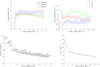 |
Fig. 1 Results for the homogenized Lindegren (2020a) data set 41,DR2 that includes more realistic uncertainties for the absolute VLBI star positions. The upper row shows the orientation and spin parameters for 38 different adjustment solutions, where for each adjustment solution the star with the largest (Qi/ni) was rejected in the following iteration. The respective (Qi/ni) and the star names are given in the lower-left plot. The lower-right plot represents the quality of the fit, equivalent to the χ2 of the adjustment, the so-called Q/n. |
4.1 Homogenized data set
Recalculating the rotation parameters using the homogenized data of the 41 stars from Sect. 2.1 and the more realistic errors from Sect. 3.2 yields scenario 41,DR2, which is pictured in Fig. 1. For completeness, the results for a scenario “41,DR2,σmodel pos” are provided in Appendix D. Both scenarios are based on the same values for the star positions. However, the star positions in 41,DR2 have uncertainties σabsolute applied, whereas those in 41,DR2 σmodel pos have only the thermal errors applied (see Sect. 3.2). The latter application is similar to the error scheme in Lindegren (2020a), but applied consistently to all stars. In total, 38 iterations were performed. In the upper two plots in Fig. 1 the results of the orientation (left) and spin (right) parameters are shown, while in the lower left plot, the max (Qi/ni) quantity along with the corresponding star names are given. The lower right plot gives information about the goodness of the fit, Q/n. All plots are relative to the number of rejected stars, k, in the iteration.
The homogenization and the more realistic error budget reduce the WRMS of the parameters by a factor of 2 to 4 for ϵY, ϵZ, ωX, and ωY when compared to the original scenario 41,DR2,Lind2020 (see Table 4). On the other hand, the parameters ϵX and ωZ are only slightly affected. The mean formal errors ME41,DR2 of the orientation parameters are 2.5–3.5 times those in scenario 41,DR2,Lind2020, whereas the mean formal errors of the spin parameters only increase marginally. The ratio between WRMS41,DR2 and ME41,DR2 is not significant for scenario 41,DR2, whereas it was significant for all orientation parameters in scenario 41,DR2,Lind2020. The t-test shows that the reduction in ϵY of 0.88 mas, and ϵZ of 0.56 mas as well as the increase in ωY of 0.07 mas yr−1 are significant.
The shifted phase-referencing calibrator positions from historical positions to ICRF3 positions are mostly less than a milliarcsecond but they have a large impact on both orientation and spin parameters, given the provided data set. In addition, the improved weighting of the model star positions by applying the calibrator catalog uncertainties homogeneously for all stars, and not a mixture of error budgets as in Lindegren (2020a), influences the resulting rotation parameters as well (see Appendix D). The change in the error budget for the positions has the largest impact on the orientation parameters. This approach reduces the Q/n quantity compared to 41,DR2,Lind2020. It now decreases below unity when k = 26 stars are rejected, compared to k = 33 rejected stars for 41,DR2,Lind2020. The plots showing the evolution of the variable max(Qi/ni) with the number of rejected stars k indicate that the order of rejected stars is almost the same.
4.2 Gaia EDR3
Also, in Gaia EDR3 no matched ICRF3 S/X radio sources are brighter than G =13 mag and optically bright radio stars are needed for the link of the bright Gaia reference frame to ICRF.
Gaia EDR3 is based on a longer observation time span than DR2, and the epoch of the catalog changed to T = 2016.0. Velocities are still only modeled linearly. Higher order terms or orbits due to multiple star systems are neglected. Therefore, differences in proper motion of Gaia EDR3 and DR2 may not only be due to better sampling but also due to nonlinear motions. The red supergiant VY CMa shows very large differences between Gaia DR2 and EDR3. Its Gaia EDR3 proper motion better matches the VLBI data in Zhang et al. (2012). In addition its negative parallax of approximately -6 mas in Gaia DR2 disappeared. Gaia EDR3 was corrected for its spin offset during the Gaia data processing. Therefore, the adjusted rotation parameters (Fig. 2) are the orientation and residual spin of the frame as determined by VLBI. The uncertainty in the Gaia EDR3 spin correction is at least 0.024 mas yr−1 per axis (Lindegren et al. 2021b).
All WM parameters change significantly in solution 41,EDR3 compared to the result for Gaia DR2 (see Table 4). The magnitude of the orientation parameters changed by 0.09 mas to 0.17 mas, and that of the spin parameters by 0.0 7mas yr−1 to 0.20 mas yr−1. The WRMS41,edr3 is between 0.079 and 0.129 mas for the orientation parameters, corresponding to 1.0to 2.5-fold the values for Gaia DR2. At the same time, their mean formal errors remain similar because the error budget for the orientation parameters is dominated by the (inflated) VLBI uncertainties. In contrast, the mean formal errors for the spin are only about 50 % of those for 41,DR2, which is expected due to smaller proper motion uncertainties in Gaia EDR3 compared to Gaia DR2 due to the longer observation time span in Gaia EDR3. Moreover, the WRMS41,EDR3 for ωZ reduced by a factor of 2.1 and that for ωX by a factor of 1.4.
WM, WRMS, and ME of the various rotation parameter scenarios.
4.3 Including the new one-epoch observations
The newly derived single-epoch star positions determined with the VLBA were inserted into the analysis. If the stars were observed relative to two different primary calibrators, both positions were employed in the adjustment. This will, if only those two positions are present, result in a WM position for the corresponding stars. For close binaries the center of luminosity was used.
Star bet Per, although successfully detected in VLBI, was not used in the adjustment. In our VLBI observations in January 2020, star betPer was scheduled although it only had a matching object in Gaia DR2 with a two parameter solution (position only). It was assumed that in Gaia EDR3 a five parameter solution would be available for the object assumed to be bet Per due to the longer data time span and therefore presumably more observations for the parameter fit. The assumption was supported by the fact that the star was also detected by its predecessor spacecraft HIPPARCOS. However, in Gaia EDR3, no counterpart was found for bet Per. This position will however be useful if comparing to future Gaia data releases, should a counterpart with a full five-parameter solution be available for the star. In total, the observations of 55 stars in both VLBI and Gaia were utilized for the adjustment of the rotation parameters. There were 21 stars that had more than one entry of positions or proper motions. Eleven stars had only a position measurement and no proper motion or parallax. Three stars had only a proper motion and parallax entry but no position. The remaining stars had one position, proper motion, and parallax entry.
Having 55 stars available, 52 iterations were run, with the same rule for star rejection as in Sect. 4.1 applied. Two solutions of the frame tie, 55,DR2 and 55,EDR3, were generated. The WM, WRMS, and ME values are given in Table 4. The respective plots for Gaia EDR3 are shown in Fig. 3. Comparing 55,EDR3 with 41,EDR3, the MEs reduce by 30–50% for the orientation parameters, and by 10 to 20% for the spin parameters. This decrease can be explained by the increase in the volume of observations. In both orientation and spin, the MEs in Y decrease most but are still the largest compared to the MEs in X and Z. For 55,EDR3 the value of unity is reached for Q/n when 15 stars are still in the sample, whereas for 41,EDR3 it is 9 stars. The WRMSs decrease by 40–50% for the orientation parameters in X and Y, while they remain similar for the other rotation parameters. The WMs change significantly (by about 0.1 mas) for parameters ϵX and ϵY.
The quantities change similarly when comparing 55,DR2 to 41,DR2. The MEs reduce by 20 to 40% for the orientation parameters, and by 10 to 20% for the spin parameters. The Q/n reaches unity when there are 9 more stars in the sample (plot not shown). The WRMSs vary very heterogeneously. For ϵX it decreases by 60%, whereas for ϵY and ϵZ it increases by 20% and 50%, respectively. For and the WRMS decreases by 35%, while it remains similar for ωY. According to the two-sample t-test introduced in Sect. 3.3, the WM changes for ϵY (−0.027 mas) and ωY (0.015 mas yr−1) are significant.
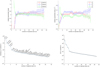 |
Fig. 2 Results for the homogenized Lindegren (2020a) data set 41,EDR3 that includes more realistic uncertainties for the absolute star VLBI positions. For a description of the plots, refer to Fig. 1. |
5 Discussion
5.1 Homogenization effect and realistic error budget
When the model positions of 29 stars were consistently referenced to the ICRF3 (scenario 41,DR2), the orientation parameters in Y and Z, and, more importantly for the frame alignment, the spin parameter in Y, were found to change significantly compared to the original scenario of Lindegren (2020a, i.e., scenario 41,DR2,Lind2020).
In this case, a spin vector with a magnitude lower than 0.1 mas yr−1, as obtained in the baseline solution of Lindegren (2020b), cannot be reached. The homogenization of the input data showed a great improvement in reducing the jumps in the orientation and spin parameters with subsequent iterations. This is a demonstration that one needs to carefully consider the systematic errors of the VLBI positions for the weighting in the frame tie determination. The effect of homogenization stresses the benefit of revisiting historical VLBI data for the alignment of Gaia to ICRF3, especially because the observations of radio stars are sparse and any systematic errors due to the use of inconsistent positions would thus likely impact the result.
In Appendix D, the results of scenario 41,DR2,σmodel pos are presented. This scenario is the same as 41,DR2, but using a VLBI position error budget based only on the uncertainties from the fit of the astrometric model and the calibrator catalog position uncertainty, applied consistently to all stars. The MEs are higher for 41,DR2 compared to 41,DR2,σmodel pos, as expected due to the inflated VLBI uncertainties. At the same time, the WRMS values in solution 41,DR2 are no better than those in solution 41,DR2,σmodel pos despite the increase in the VLBI position uncertainties – in details, the WRMS values are slightly better for ϵX, ϵY, and ωX (by 10% at most) but are 15–35 % worse for ϵZ, ωY, and ωZ. The number of rejected stars to obtain Q/n = 1, changes from 29 in 41,DR2,σmodel pos to 26 in 41,DR2, a difference that can be expected just from the inflated VLBI position uncertainties in 41,DR2. In all, the differences between solutions 41,DR2,σmodel pos and 41,DR2 are not that marked – the major changes happen when going from solution 41,DR2,Lind2020 to 41,DR2,σmodel pos. The correlation coefficients between the three orientation parameters are all above 0.5 for 41,DR2,σmodel pos, whereas they are reduced by 0.1–0.2 for 41,DR2. These reduced correlations may explain the significant change in ϵX (0.038 in scenario 41,DR2 vs. −0.152 in scenario 41,DR2,σmodel pos), whereas all other parameters are similar.
5.2 Alignment of Gaia DR2 and adding new one-epoch positions
Given the variability of our iteration solutions, the question arises as to how a baseline solution (i.e., a selected iteration solution from one scenario) can be selected. For this purpose, it is best to choose an iteration solution with as many stars as possible involved, but when a somewhat steady solution is reached – that means, after which the fluctuation of the rotation parameters lies within their level of uncertainties. On the other hand, Q/n should not deviate largely with respect to the next iteration solution anymore, and because Qi/ni may reflect the influence of binarity and radio-optical position offsets of the stars, it should be made sure that the stars with excessively large values of Qi/ni are not included.
In the case of 41,DR2, if a baseline solution had to be chosen, the one with k = 9 rejected stars would be selected. This is because the above mentioned metrics, the rotation parameter offsets, the Q/n, and the Qi/ni, do not show large jumps anymore when rejecting even more stars. The rotation parameters from this baseline solution are provided in TableE.4. The Q/n for this solution is 4.75, slightly lower than the value in Lindegren (2020b) of 5.68. However, if rejecting 15 stars as done in Lindegren (2020b), the Q/n from our solution would be as low as 2.26, which reflects the improvement resulting from the homogenization and the increase in uncertainties for the absolute positions in scenario 41,DR2. The correlation coefficients between the rotation parameters from the baseline solution are
corr[ϵX(T), ϵY(T), ϵZ(T), ωX, ωY, ωZ] =
![Mathematical equation: $\left[ {\matrix{ { + 1.000} \hfill & { + 0.419} \hfill & { + 0.276} \hfill & { + 0.173} \hfill & { + 0.119} \hfill & { + 0.031} \hfill \cr \ldots \hfill & { + 1.000} \hfill & { + 0.372} \hfill & { + 0.052} \hfill & { + 0.315} \hfill & { + 0.046} \hfill \cr \ldots \hfill & \ldots \hfill & { + 1.000} \hfill & { + 0.033} \hfill & { + 0.125} \hfill & { + 0.113} \hfill \cr \ldots \hfill & \ldots \hfill & \ldots \hfill & { + 1.000} \hfill & { 0.007} \hfill & { + 0.345} \hfill \cr \ldots \hfill & \ldots \hfill & \ldots \hfill & \ldots \hfill & { + 1.000} \hfill & { 0.065} \hfill \cr \ldots \hfill & \ldots \hfill & \ldots \hfill & \ldots \hfill & \ldots \hfill & { + 1.000} \hfill \cr } } \right]$](/articles/aa/full_html/2023/08/aa40266-20/aa40266-20-eq26.png) (15)
(15)
which shows that the orientation parameters are still weakly correlated (correlation coefficients up to 0.4). The largest changes in correlation coefficient compared to the Lindegren (2020b) baseline solution happened for that between the orientation and spin parameters in Y (increase by 0.184), and for that between the Y and Z orientation parameters (increase by 0.166).
For scenario 55,DR2 the baseline solution can be the one when rejecting k =11 stars, as listed in Table E.4. The rotation parameters agree with each other for the baseline solutions from the scenarios 41,DR2 and 55,DR2, but there is an improvement in their uncertainties for the scenario 55,DR2. The correlation coefficients between the rotation parameters from the baseline solution are
corr[ϵX(T), ϵY(T), ϵZ(T), ωX, ωY, ωZ] =
![Mathematical equation: $\left[ {\matrix{ { + 1.000} \hfill & { + 0.246} \hfill & { + 0.248} \hfill & { 0.044} \hfill & { 0.038} \hfill & { 0.040} \hfill \cr \ldots \hfill & { + 1.000} \hfill & { + 0.178} \hfill & { 0.014} \hfill & { 0.118} \hfill & { 0.013} \hfill \cr \ldots \hfill & \ldots \hfill & { + 1.000} \hfill & { 0.052} \hfill & { + 0.011} \hfill & { 0.133} \hfill \cr \ldots \hfill & \ldots \hfill & \ldots \hfill & { + 1.000} \hfill & { 0.004} \hfill & { + 0.290} \hfill \cr \ldots \hfill & \ldots \hfill & \ldots \hfill & \ldots \hfill & { + 1.000} \hfill & { 0.046} \hfill \cr \ldots \hfill & \ldots \hfill & \ldots \hfill & \ldots \hfill & \ldots \hfill & { + 1.000} \hfill \cr } } \right]$](/articles/aa/full_html/2023/08/aa40266-20/aa40266-20-eq27.png) (16)
(16)
As shown in this matrix, there are only negligible correlations between the rotation parameters (correlation coefficients smaller than 0.3).
In 55,DR2, the weights of the stars used for solving for the spin are similar to those in scenario 41,DR2,Lind2020, ranging from 0.68 mas−2 yr2 to 910 mas−2 yr2 with a median of 107 mas−2 yr2. The group of stars having the largest weights is the same as that in 41,DR2 and 41,DR2,Lind2020 (see Lindegren 2020b). The weights of the stars used for solving for the orientation, however, reduce substantially to be within the range of 0.01 mas−2 to 54 mas−2, with a median of 9 mas−2. This means that the corresponding stars more evenly contribute to the orientation estimates compared to 41,DR2,Lind2020, where the range of weights was 0.2 mas−2 to 1156 mas−2. The contribution to the determination of the orientation parameters with the highest weights are from the stars reobserved in the January 2020 sessions.
For 55,DR2, we also tried employing the barycenter instead of the center of luminosity as a reference point for the new observations of the close unresolved binaries in Table 3 to investigate which center is closer to the Gaia photocenter. The differences in the residuals for the astrometric parameters are similar to the position differences between the two centers in Table 3. The residuals are not systematically smaller for either center. However, the study may be biased because the historical positions of the three binary stars (from Lindegren 2020a) included in the VLBI data set have not been changed. A more detailed study needs to be carried out to investigate the change from the barycenter to the center of luminosity also for the historical data. The proper motion values and uncertainties did not change between Lindegren (2020b) and our work. Thus, if the spin were determined only from the proper motion information, it would be the same when using the proper motions of either the 55,DR2 or the 41,DR2,Lind2020 data set. The latter is scenario B in Lindegren (2020b) and the determined spin is (-0.050, -0.139, 0.002) ± (0.036, 0.055, 0.038) mas yr−1. The spin from the baseline solution of 55,DR2 (including the information coming from the positions) that is reported in Table E.4 can thus be compared directly to the spin from scenario B to see if the positions have an effect on the determination of the spin. The comparison shows that the spin parameters from the two solutions differs by less than 1σ. However, their uncertainties are about halved in the case of 55,DR2, meaning that the addition of the positions allows the determination of the spin to be improved. For the spin in Y, our baseline solution (−0.113 ± 0.024 mas yr−1) is closer to scenario B than to the baseline solution of 41,DR2,Lind2020 (−0.051 ± 0.027 mas yr−1, equivalent to scenario A in Lindegren 2020b). Compared to 41,DR2,Lind2020, the positions in 55,DR2 were given lower weights relative to the proper motion information because of inflated uncertainties. However, the effect of the inflated position uncertainties was compensated by the increased number of star positions so that the formal errors for the spin parameters in 55,DR2 are similar to those of the original baseline solution 41,DR2,Lind2020.
Another possibility to assess the results of the homogenization effort and the new one-epoch positions is to compare with other results from the literature. Brandt (2018) derived proper motions of 115 662 stars by dividing the differences of positions from Gaia DR2 and HIPPARCOS by the time difference of their respective epochs, which is 24.25 yr. In addition, he reduced systematics by cross-calibrating these proper motions with the proper motions from the Gaia and HIPPARCOS catalogs themselves. This includes the correction of global rotations between the catalogs. The spin parameters he derived are (ωX, ωY, ωZ) = (−0.081, −0.113, −0.038) mas yr−1. Lindegren (2020a) estimated the corresponding uncertainties to be 0.03 mas yr−1. Brandt’s spin parameters for Gaia DR2 must be corrected for the orientation offset between the Gaia DR2 bright frame and ICRF3 in order to compare them to the spin parameters of 55,DR2. This requires adding the orientation parameters of 55,DR2 divided by the time difference of 24.25 yr to the spin parameters of Brandt (2018; Lindegren 2020a). The corrected spin parameters are (ωX, ωY, ωZ) = (−0.077, −0.094, −0.037)±(0.026, 0.026, 0.025) mas yr−1. Comparing with the values for 55,DR2 in Table E.4, the differences are at the level of 0.7σ, 0.5σ, and 2.1σ, thus showing reasonably good agreement between the two determinations.
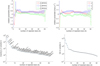 |
Fig. 3 Results for Gaia EDR3 in scenario 55,EDR3 when using the homogenized data set described in Sect. 2.1 as well as the new data acquired for this work as explained in Sect. 2.2, with the more realistic errors from Sect. 3.2 applied. For a description of the plots, refer to Fig. 1. |
5.3 Alignment of Gaia EDR3
The iteration that rejects the 13 most deviating stars is selected as a new baseline solution for 55,EDR3 as given in Table E.4. The uncertainties show a similar behavior as those predicted by Lindegren (2020b) that is that the spin parameter uncertainties should decrease in future Gaia data releases, even without adding further VLBI observations. This is due to smaller uncertainties in the Gaia EDR3 positions and proper motions. However, the Q/n equals 5.58 for this solution, which is larger than that for the baseline solution of 55,DR2 at iteration k = 13 (4.63), thus signalizing the presence of systematic errors. The correlation coefficients between the rotation parameters from the baseline solution are
corr[ϵX(T), ϵY (T), ϵZ (T), ωX, ωY, ωZ] =
![Mathematical equation: $\left[ {\matrix{ { + 1.000} \hfill & { + 0.225} \hfill & { + 0.212} \hfill & { + 0.200} \hfill & { + 0.024} \hfill & { 0.003} \hfill \cr \ldots \hfill & { + 1.000} \hfill & { + 0.177} \hfill & { + 0.021} \hfill & { + 0.177} \hfill & { + 0.010} \hfill \cr \ldots \hfill & \ldots \hfill & { + 1.000} \hfill & { 0.007} \hfill & { + 0.039} \hfill & { + 0.023} \hfill \cr \ldots \hfill & \ldots \hfill & \ldots \hfill & { + 1.000} \hfill & { + 0.044} \hfill & { + 0.326} \hfill \cr \ldots \hfill & \ldots \hfill & \ldots \hfill & \ldots \hfill & { + 1.000} \hfill & { + 0.018} \hfill \cr \ldots \hfill & \ldots \hfill & \ldots \hfill & \ldots \hfill & \ldots \hfill & { + 1.000} \hfill \cr } } \right]$](/articles/aa/full_html/2023/08/aa40266-20/aa40266-20-eq28.png) (17)
(17)
Only negligible correlations (i.e., correlation coefficients smaller than 0.3) among the rotation parameters are present except between ωX and ωZ.
For the bright reference frame, a correction was applied to its spin in one of the middle iterations of the Gaia EDR3 processing (Lindegren et al. 2021b). The correction was derived through comparing the proper motions of Gaia EDR3 at that iteration step with those obtained by dividing the position differences between Gaia DR2 and HIPPARCOS by the epoch difference of the two catalogs. The applied spin correction is (−0.0166, −0.0950, +0.0283) mas yr−1. No orientation offset could be applied due to the lack of suitable data to compare with. Due to the involvement of HIPPARCOS positions in the calculations and their ±0.6mas uncertainties in aligning to ICRS at epoch J1991.25, the spin of the bright reference frame of Gaia EDR3 cannot be determined to better than about 0.024 mas yr−1 per axis using this method (Lindegren et al. 2021b). This is about twice as large as the formal errors of the spin parameters derived in this study. Due to the applied correction, the result of 55,EDR3 can be understood as the residual spin of the corrected Gaia bright frame. The residual spin is determined to be significant at the 2.4σ level in Y (+0.065±0.026 mas yr−1 when the scaling factor  is applied). Reversing the applied correction by adding it back to the baseline solution results in an original, uncorrected spin in Gaia EDR3 of (+0.005, −0.030, +0.012) ± (0.024, 0.026, 0.024) mas yr−1. Our study thus suggests that the uncorrected bright Gaia EDR3 frame is more consistent with the ICRF3 than the corrected frame and thus that the spin correction based on HIPPARCOS had better not been applied in the Gaia EDR3 processing.
In terms of precision, the current tie of the bright reference frame of Gaia to ICRF3 is not yet at the required level. For example, the formal errors of the spin parameters for 55,EDR3 are about 0.01 mas yr−1, which is five times the anticipated 0.002 mas yr−1 proper motion uncertainty for a single star in the final Gaia data release7, and the WRMS55,EDR3 values are even larger (see Table 4). Moreover, the parameter estimates do not appear to be very robust (see, e.g., the steadiness of the spin parameters in Fig. 3). Comparing with Gaia DR2, the mean errors of the spin parameters are reduced by 50%, an effect due to the increased time span for Gaia EDR3, while the mean errors for the orientation parameters remain similar. The WRMS values for Gaia EDR3 remain at the same level as that in Gaia DR2, or even increase, except for ωZ. For 55,EDR3, Q/n becomes smaller than unity at k = 40, where 15 stars are still included, while for 55,DR2 the value of 1 is reached for k = 35, while 20 stars are still included. In all, the increased time span for Gaia EDR3 does not translate into an improved frame tie, which indicates that the limitation most probably comes from the VLBI data. Further VLBI observational efforts are therefore highly desirable to improve the current situation.
The residuals of the position and proper motion differences between VLBI and Gaia are plotted in Fig. 4 for the baseline solution of 55,DR2 and in Fig. 5 for the baseline solution of 55,EDR3. Apart from a few outliers, most residuals remain within twoto three-fold their uncertainties. The improvement of the Gaia proper motion for VY CMa is confirmed. The plots show that the large residuals generally correspond to the stars that have VLBI positions determined from observations at epochs far away from the Gaia epoch. This finding suggests that it is best to have VLBI observations concentrated during the Gaia observation period.
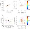 |
Fig. 4 Residuals of the differences of the positions and proper motions between VLBI and Gaia after adjustment of the orientation and spin between the two reference frames. Results are given for the baseline solution of 55,DR2 described in Table E.4. Individual values are color coded by the epoch of the VLBI position. The lower plots show zoomedin views of the central area of the upper plots. The position residuals for T Tau and S Crt are not shown, as they are outside the plotted area. The residuals for VY CMa are marked with a black diamond. |
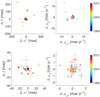 |
Fig. 5 Residuals of the differences of the positions and proper motions between VLBI and Gaia after adjustment of the orientation and spin between the two reference frames. Results are given for the baseline solution of 55,EDR3 described in Table E.4. See Fig. 4 for a description of the plot. |
6 Conclusion and outlook
In this work we have evaluated and extended the determination of the orientation and spin of the optically bright (G ≤ 13 mag) Gaia reference frame with respect to the ICRF3 as introduced by Lindegren (2020a). We homogenized the data collected in Lindegren (2020a) so that all star positions refer to the ICRF3 and have consistent uncertainties based on the position uncertainty of the calibrators in the ICRF3. Additionally, newly acquired VLBA observations allowed for the detection of 32 stars. The resulting radio positions of these stars were used in our study together with the historical data to further constrain the tie between the two frames. An attempt was also made to evaluate the error budget of the radio positions of the stars with respect to the ICRF3 in order to derive more realistic weights for these positions, which should help further improve the frame tie.
Our study has led to more stable parameter estimates in the iterative process, in which the most divergent star is rejected at each iteration. Moreover, the bright reference frame of Gaia DR2, which is estimated to be offset by about 1.3 mas in the Y direction and 0.6 mas in the Z direction by Lindegren (2020b), is now found to agree with the ICRF3 within 0.5 mas in any direction. On the other hand, its spin component in the Y direction is found to be significant at the 2σ level. The newly determined radio positions of 32 stars reduce the correlations among the rotation parameters. Our study further suggests that the bright reference frame of Gaia EDR3 is consistent in orientation with the ICRF3 within about 0.3 mas, while its rotation rate is statistically significant, with a magnitude of 0.065 ±0.026 mas yr−1 in the Y direction.
Additional VLBI observations, particularly of new stars, will help reduce the formal error of the orientation parameters. The orientation in the Y direction is still the least well determined for both Gaia DR2 and Gaia EDR3. The observations should be conducted in the immediate future, as observations close to the final Gaia epoch will help reduce the formal errors of the orientation parameters most (Lindegren 2020a).
As the optical positions and proper motions of the radio stars will continue to be improved by Gaia in the near future, the result of the frame tie will be primarily affected by the astrophysical nature of these stars and the systematic errors in their radio positions with respect to the ICRF3. Although we made an attempt to carefully consider the systematic errors in the process of deriving the results, they are source-dependent and should be assessed on a case-by-case basis. To reduce the impact, it is desirable to acquire further VLBI observations of the known and new stars on a regular basis in the future.
Both data entries were used for this work to be consistent with Lindegren (2020a).
We corrected the u, v, w terms of the target stars to match the position of the brightest peak in the images created from the uncorrected data by using task UVFIX in AIPS. This allowed all channels of each subband to be combined, which is needed for DIFMAP, without loss of S/N due to potential bandwidth smearing in case the a priori position of the target star deviated from the approximate positions used for correlation by more than several tens of mas.
Dynamic range is defined as the ratio of the peak intensity to the image noise level.
Acknowledgements
We are grateful for the helpful support of F. Schinzel (NRAO) during AIPS data processing. We deeply thank the anonymous referee for constructive suggestions to improve the content and readability of the manuscript. The authors acknowledge use of the Very Long Baseline Array under the US Naval Observatory’s time allocation. This work supports USNO’s ongoing research into the celestial reference frame and geodesy. We thank also the Socorro correlator for reliably and quickly providing the correlated data. The National Radio Astronomy Observatory is a facility of the National Science Foundation operated under cooperative agreement by Associated Universities, Inc. This project is supported by the DFG grants no. SCHU 1103/7-2 and no. HE 5937/2-2. M.H. Xu was supported by the Academy of Finland project no. 315721. This work has made use of the data from the European Space Agency (ESA) mission Gaia processed by the Gaia Data Processing and Analysis Consortium as well as from the mission HIPPARCOS. Funding for the DPAC has been provided by national institutions, in particular the institutions participating in the Gaia Multilateral Agreement. Calibrators were selected using the NRAO VLBA calibrator search tool (www.vlba.nrao.edu/astro/calib/), the RFC calibrator search tool (www.astrogeo.org/calib/search.html), and the Astrogeo VLBI FITS image database (www.astrogeo.org/vlbi_images/). This research has made use of the VizieR catalog access tool, CDS, Strasbourg, France and the SIMBAD database (Wenger et al. 2000), operated at CDS, Strasbourg, France. Calculations were made in MATLAB which is distributed by the MathWorks, Inc.
Appendix A Selection of candidate stars and calibrators for new observations
After collecting suitable VLBI data of stars from relevant literature, we conducted a crossmatch between VLBI and Gaia by exploiting capabilities of the Gaia archive8 in order to identify counterparts. We mainly made use of the literature collections of Lindegren (2020a), as well as Xu et al. (2019b), and references therein. Stars that are probably not suitable for the radio-optical link, such as Mira-type stars and red supergiants (Lindegren 2020a) and stars of spectral types other than A, F, G, and K (Lindegren, June 2019, priv. comm.), were rejected. The sample was restricted to stars brighter than G =13 mag having a full 5-parameter solution in DR2. Furthermore, only objects with declinations above -30° were considered because of the declination limit of the VLBA.
Using the RUWE parameter (calculated from Gaia DR2 data; Lindegren et al. 2018), we selected stars that were not indicated to be resolved binaries in DR2. For groups of stars within a few degrees on the sky, we selected only the brightest stars at radio frequencies, as multiple detections clustered in one part of the sky are geometrically worse for the determination of the rotation parameters than spreading the observations over the whole sky considering limited telescope time availability. Nine stars were included in the observation proposal although they do not fully meet all selection criteria. Among these are, σ2 CrB and UX Ari, which were excluded in the analysis of Lindegren (2020b) because they show evidence for a binary companion. However, they are well observed objects in Lestrade et al. (1999), and therefore by extending their position time series with just a few new observations, highly accurate proper motions in the radio frame can be derived along with any nonlinear orbital motions if necessary. Plots of the sky and magnitude coverage of the selected subset, as well as further information on selection criteria, can be found in Lunz et al. (2020). In total 46 stars were chosen as candidates for re-observation.
Criteria for scheduling phase-referencing observations in nodding-style described in Wrobel et al. (2000) were considered. Phase-referencing calibrators that are compact, radio-bright, and close in direction to the target stars were selected, and the ideal switching times between the calibrators and targets were determined. In case historical data used a different calibrator, we added the original phase-referencing calibrator whenever appropriate. In addition, secondary calibrators were chosen whenever possible. These can be utilized for removing residual phasegradients during the data processing. The recommendations of geometrical arrangements of the secondary calibrators with respect to the primary calibrator and star in Fomalont & Kogan (2005) were followed. Sometimes there were no other suitable calibrators available, whereupon no secondary calibrator was selected.
Appendix B Peak intensities
For the derivation of peak intensities, phaseand amplitude-selfcalibration was performed in AIPS on the phase-referencing calibrator P 1 (see Table 1). With this step, absolute positional information is lost, but the dynamic range in the images increases. More importantly, the phase coherence for the target star is improved, and the accuracy of the flux density measurement is increased. The derived corrections of phase and amplitude were applied to the respective target stars, the secondary calibrators, and the phase-referencing calibrator itself, in the multisource file. Then, the target stars and secondary calibrators were split and imaged again as described above. If necessary and possible, phase-only self calibration was performed on the target and secondary calibrators afterward. At the end, the peak flux densities of all objects were determined using the task JMFIT on the brightest component based on the image. For the star del Lib, the radio source J1456-0617 was used as the final phase-referencing calibrator because it had more valid fringes than J1510-0843.
For the detected stars and their calibrators, the peak intensities P I are listed in Table B.1. The mean (median) peak intensity for the detected target stars is 11 (1.5) mJy beam−1. Their mean (median) standard deviation σΡΙ, which represents the RMS noise of the images, is 0.17 (0.09) mJy beam−1. Dynamic ranges DR vary from 5.5 for star SV Cam to 349.6 for SZ Psc.
Peak intensities for the 32 detected stars and their calibrators from the VLBA observations conducted on 6–7 January 2020.
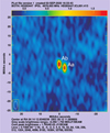 |
Fig. C.1 Phase-referenced map of star HD 283447. Self-calibration was performed on the calibrator J0408+3032 and applied to the star. The labels Aa and Ab identify the components of subsystem A. |
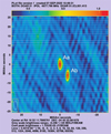 |
Fig. C.2 Phase-referenced map of star Do Ar 51. Self-calibration was performed on the calibrator J1633−2557 and applied to the star. The labels Aa and Ab identify the components of subsystem A. |
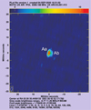 |
Fig. C.3 Phase-referenced map of star UX Ari. Self-calibration was performed on the calibrator J0316+2733 and applied to the star. The labels Aa and Ab identify the components of the close binary subsystem A. |
Appendix C Identification of close binaries
The VLBI images in Figs. C1, C.2, and C.3 show that three of our stars are resolved close binaries. Stars HD 283447 (V773 Tau) and DoAr 51 (V2248 Oph) consist of two close components of almost equal peak intensity. As Torres et al. (2012) summarize, HD 283447 is at least a quadruple system. The subsystem HD 283447 A is a strong radio source and a spectroscopic binary consisting of components Aa and Ab (Phillips et al. 1996; Boden et al. 2007; Massi et al. 2008). Its trajectory is gravitationally influenced by the other components of the system, mainly by subsystem HD 283447 Β, which has an apparent separation of about 150 mas. From comparison of Fig. C.1 with the orbit (Fig. 4 of Torres et al. 2012), it could be determined that the west (right) component is the primary component Aa, and the east (left) component is the secondary component Ab. DoAr 51 is a triple system with a close binary of about 60 mas maximum separation and a third component about 078 away (Barsony et al. 2003; Ortiz-Leon et al. 2017b). From comparison of the image in Fig. C.2 with the orbit in Fig. 3 of Ortiz-Leon et al. (2017b), it could be determined that the east (left) component is the primary component Aa, and the west (right) component is the secondary component Ab. For UX Ari, structure was detected, as shown in Fig. C.3, which could represent the inner close binary system A of the triple system described in Hummel et al. (2017). Then the stronger eastern (left) component is the subgiant primary star Aa, and the weaker western (right) component is its main-sequence companion Ab as reported in Carlos & Popper (1971). JMFIT was unable to fit two separate Gaussians, which is why only one component is shown in Table B.1.
Appendix D Rotation parameter solution using homogenized positions and uncertainties for the calibrators
The recalculation of the rotation parameters as in Fig. 3 in Lindegren (2020b), but using homogenized positions and uncertainties for the 41 stars from Sect. 2.1, yields scenario 41,DR2,σmodel pos for the Gaia DR2 analysis (Fig. D.l).
The metrics for the evaluation of the iterative solutions are shown in Table D.1. For comparison, the same metrics for scenario 41,DR2,Lind2020 from the original data published in Lindegren (2020a) are shown in Table 4. The homogenization of the positions and uncertainties reduces the WRMS of all parameters except ϵX. In particular, the WRMS decreases by a factor of 2 to 4 for ϵY, ϵZ, ωX, and ωY. At the same time, the formal errors of the orientation parameters are increased by a factor of 1.5 to 2 while the formal errors of the spin parameters are only marginally affected. Except for ϵX, the WRMSs are equal or smaller than the MEs, whereas they were larger (by up to a factor of 3.5) in scenario 41,DR2,Lind2020. The plots in Fig. D.1 confirm that the solutions of the iterations become steadier for most rotation parameters.
The large orientation offset about the Y axis (1.273 mas) reduces to about one third of its original value (0.393 mas), and the one about the Ζ axis (0.537 mas) vanishes, while ϵX remains small (−0.152 mas). In contrast, the magnitude of the spin parameters along the three axes increase. The differences in orientation and spin except for ωZ are statistically significant applying the t-test.
The parameter Q/n is below unity with k = 29 rejected stars in this scenario compared to k = 33 rejected stars in scenario 41,DR2,Lind2020, which shows that the VLBI and Gaia data sets align better for more stars now. The order of the rejected stars is almost the same.
WM, WRMS, and ME of the rotation parameters in scenario 41,DR2,σmodel pos
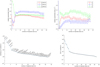 |
Fig. D.1 Results for the homogenized Lindegren (2020a) data set 41,DR2,σmodel pos. The upper row shows the orientation and spin parameters for 38 different adjustment solutions, where for each adjustment solution the star with the largest (Qi/ni) was rejected in the following iteration. The respective (Qi/ni) and the star names are given in the lower-left plot. The lower-right plot represents the quality of the fit, equivalent to the χ2 of the adjustment, the so-called Q/n. |
Appendix E Tables
Subset of stars from Table 1 of Lindegren (2020a) along with the corresponding phase-referencing calibrators and the corrections to be applied in order to homogenize the data set.
Date and time of experiments.
Positions estimated for the 32 radio stars detected with the VLBA on 6–7 January 2020, along with the respective phase-referencing calibrators used.
Notes. The apparent star-calibrator separation is Δc. Uncertainties σα*,random and σδ,random refer to the random error from observations, whereas σα*,absolute and σδ,absolute are inflated uncertainties as described in Sect. 3.2. The parameters Roe (t), Δα(t), and Δδ(t) need to be applied if the effect of parallax should be corrected. Thereby, the Römer delay Roe needs to be subtracted from the epoch t in column 4, which is the mean epoch between the first and the last scans. In addition, the parallax effects Δα, and Δδ need to be added to the positions in Cols. 5 and 8. The last column shows the radial velocity (υr) taken from SIMBAD and used in the rotation parameter calculation.
Baseline solutions for various scenarios.
References
- Andrei, A. H., Jilinski, E. G., & Puliaev, S. P. 1995, AJ, 109, 428 [NASA ADS] [CrossRef] [Google Scholar]
- Arenou, F., Luri, X., Babusiaux, C., et al. 2018, A&A, 616, A17 [NASA ADS] [CrossRef] [EDP Sciences] [Google Scholar]
- Arias, E. F., Charlot, P., Feissel, M., & Lestrade, J. F. 1995, A&A, 303, 604 [NASA ADS] [Google Scholar]
- Asaki, Y., Deguchi, S., Imai, H., et al. 2010, ApJ, 721, 267 [NASA ADS] [CrossRef] [Google Scholar]
- Barsony, M., Koresko, C., & Matthews, K. 2003, ApJ, 591, 1064 [NASA ADS] [CrossRef] [Google Scholar]
- Bartel, N., Bietenholz, M. F., Lebach, D. E., et al. 2015, Class. Quant. Grav., 32, 224021 [NASA ADS] [CrossRef] [Google Scholar]
- Boboltz, D. A., Fey, A. L., Puatua, W. K., et al. 2007, AJ, 133, 906 [NASA ADS] [CrossRef] [Google Scholar]
- Boden, A. F., Torres, G., Sargent, A. I., et al. 2007, ApJ, 670, 1214 [NASA ADS] [CrossRef] [Google Scholar]
- Brandt, T. D. 2018, ApJS, 239, 31 [Google Scholar]
- Carlos, R. C., & Popper, D. M. 1971, PASP, 83, 504 [NASA ADS] [CrossRef] [Google Scholar]
- Charlot, P., Jacobs, C. S., Gordon, D., et al. 2020, A&A, 644, A159 [EDP Sciences] [Google Scholar]
- Clark, B. G. 1980, A&A, 89, 377 [NASA ADS] [Google Scholar]
- Condon, J. J. 1997, PASP, 109, 166 [NASA ADS] [CrossRef] [Google Scholar]
- de Bruijne, J. H. J., Rygl, K. L. J., & Antoja, T. 2014, in EAS Publications Series, 67-68, 23 [Google Scholar]
- ESA 1997, The Hipparcos and Tycho catalogues. Astrometric and photometric star catalogues derived from the ESA Hipparcos Space Astrometry Mission, ESA Special Publication, 1200 [Google Scholar]
- Folkner, W. M., Williams, J. G., & Boggs, D. H. 2009, IPN Progress Report, 178 [Google Scholar]
- Fomalont, E., & Kogan, L. 2005, AIPS Memo 111, NRAO [NASA ADS] [Google Scholar]
- Fomalont, E., Johnston, K., Fey, A., et al. 2011, AJ, 141, 91 [NASA ADS] [CrossRef] [Google Scholar]
- Gaia Collaboration (Brown, A. G. A., et al.) 2016a, A&A, 595, A2 [NASA ADS] [CrossRef] [EDP Sciences] [Google Scholar]
- Gaia Collaboration (Prusti, T., et al.) 2016b, A&A, 595, A1 [NASA ADS] [CrossRef] [EDP Sciences] [Google Scholar]
- Gaia Collaboration (Brown, A. G. A., et al.) 2018, A&A, 616, A1 [NASA ADS] [CrossRef] [EDP Sciences] [Google Scholar]
- Gaia Collaboration, (Brown, A. G. A., et al.) 2021a, A&A, 649, A1 [NASA ADS] [CrossRef] [EDP Sciences] [Google Scholar]
- Gaia Collaboration (Klioner, S. A., et al.) 2021b, A&A, 649, A9 [EDP Sciences] [Google Scholar]
- Galli, P. A. B., Loinard, L., Ortiz-Léon, G. N., et al. 2018, ApJ, 859, 33 [Google Scholar]
- Gattano, C., Lambert, S. B., & Le Bail, K. 2018, A&A, 618, A80 [NASA ADS] [CrossRef] [EDP Sciences] [Google Scholar]
- Greisen, E. W. 2003, in Information Handling in Astronomy Historical Vistas, 285, ed. A. Heck (Astrophys and Space Sci Lib: Springer Netherlands), 109 [NASA ADS] [CrossRef] [Google Scholar]
- Högbom, J. A. 1974, A&As, 15, 417 [Google Scholar]
- Hummel, C. A., Monnier, J. D., Roettenbacher, R. M., et al. 2017, ApJ, 844, 115 [NASA ADS] [CrossRef] [Google Scholar]
- Jones, D. L., Folkner, W. M., Jacobson, R. A., et al. 2020, AJ, 159, 72 [NASA ADS] [CrossRef] [Google Scholar]
- Kettenis, M., van Langevelde, H. J., Reynolds, C., & Cotton, B. 2006, in Astronomical Data Analysis Software and Systems XV, eds. C. Gabriel, C. Arviset, D. Ponz, & S. Enrique, Astronomical Society of the Pacific Conference Series, 351, 497 [NASA ADS] [Google Scholar]
- Kounkel, M., Hartmann, L., Loinard, L., et al. 2017, ApJ, 834, 142 [Google Scholar]
- Kovalev, Y. Y., Lobanov, A. P., Pushkarev, A. B., & Zensus, J. A. 2008, A&A, 483, 759 [NASA ADS] [CrossRef] [EDP Sciences] [Google Scholar]
- Kusuno, K., Asaki, Y., Imai, H., & Oyama, T. 2013, ApJ, 774, 107 [NASA ADS] [CrossRef] [Google Scholar]
- Lestrade, J. F., Preston, R. A., Jones, D. L., et al. 1999, A&A, 344, 1014 [NASA ADS] [Google Scholar]
- Lindegren, L. 2020a, A&A, 633, A1 [Google Scholar]
- Lindegren, L. 2020b, A&A, 637, A5 [NASA ADS] [CrossRef] [EDP Sciences] [Google Scholar]
- Lindegren, L., Lammers, U., Bastian, U., et al. 2016, A&A, 595, A4 [NASA ADS] [CrossRef] [EDP Sciences] [Google Scholar]
- Lindegren, L., Hernández, J., Bombrun, A., et al. 2018, A&A, 616, A2 [NASA ADS] [CrossRef] [EDP Sciences] [Google Scholar]
- Lindegren, L., Bastian, U., Biermann, M., et al. 2021a, A&A, 649, A4 [EDP Sciences] [Google Scholar]
- Lindegren, L., Klioner, S. A., Hernández, J., et al. 2021b, A&A, 649, A2 [EDP Sciences] [Google Scholar]
- Loinard, L., Torres, R. M., Mioduszewski, A. J., et al. 2007, ApJ, 671, 546 [NASA ADS] [CrossRef] [Google Scholar]
- Lunz, S., Heinkelmann, R., Anderson, J., et al. 2019, Radio source position offsets among various radio frames and Gaia [Google Scholar]
- Lunz, S., Heinkelmann, R., Anderson, J., et al. 2020, in Astrometry, Earth Rotation, and Reference Systems in the GAIA era, ed. C. Bizouard, 49 [Google Scholar]
- MacMillan, D. S., Fey, A., Gipson, J. M., et al. 2019, A&A, 630, A93 [NASA ADS] [CrossRef] [EDP Sciences] [Google Scholar]
- Martí-Vidal, I., Ros, E., Pérez-Torres, M. A., et al. 2010, A&A, 515, A53 [NASA ADS] [CrossRef] [EDP Sciences] [Google Scholar]
- Martí-Vidal, I., Ros, E., Pérez-Torres, M. A., et al. 2011, A&A, 533, C1 [NASA ADS] [CrossRef] [EDP Sciences] [Google Scholar]
- Martin-Mur, T. J., Zhai, C., Jacobs, C., et al. 2017, in 2017 IEEE International Conference on Space Optical Systems and Applications (ICSOS), 176 [CrossRef] [Google Scholar]
- Massi, M., Ros, E., Menten, K. M., et al. 2008, A&A, 480, 489 [NASA ADS] [CrossRef] [EDP Sciences] [Google Scholar]
- Miller-Jones, J. C. A., Sivakoff, G. R., Knigge, C., et al. 2013, Science, 340, 950 [NASA ADS] [CrossRef] [Google Scholar]
- Mioduszewski, A. J. 2009, AIPS Memo 110 [Google Scholar]
- Nakagawa, A., Tsushima, M., Ando, K., et al. 2008, PASJ, 60, 1013 [NASA ADS] [Google Scholar]
- Nakagawa, A., Omodaka, T., Handa, T., et al. 2014, PASJ, 66, 101 [NASA ADS] [CrossRef] [Google Scholar]
- Nyu, D., Nakagawa, A., Matsui, M., et al. 2011, PASJ, 63, 63 [NASA ADS] [CrossRef] [Google Scholar]
- Ortiz-León, G. N., Dzib, S. A., Kounkel, M. A., et al. 2017a, ApJ, 834, 143 [Google Scholar]
- Ortiz-León, G. N., Loinard, L., Kounkel, M. A., et al. 2017b, ApJ, 834, 141 [Google Scholar]
- Peterson, W. M., Mutel, R. L., Lestrade, J.-F., Güdel, M., & Goss, W. M. 2011, ApJ, 737, 104 [NASA ADS] [CrossRef] [Google Scholar]
- Petrov, L. 2018, VLBI global solution 2018b, http://astrogeo.org/sol/rfc/rfc_2018b/, accessed 2019-06-12 [Google Scholar]
- Phillips, R. B., Lonsdale, C. J., Feigelson, E. D., & Deeney, B. D. 1996, AJ, 111, 918 [NASA ADS] [CrossRef] [Google Scholar]
- Porcas, R. W. 2009, A&A, 505, L1 [NASA ADS] [CrossRef] [EDP Sciences] [Google Scholar]
- Pradel, N., Charlot, P., & Lestrade, J.-F. 2006, A&A, 452, 1099 [NASA ADS] [CrossRef] [EDP Sciences] [Google Scholar]
- Reid, M., & Honma, M. 2014, ARA&A, 52, 339 [NASA ADS] [CrossRef] [Google Scholar]
- Riess, A. G., Casertano, S., Yuan, W., et al. 2018, ApJ, 861, 126 [NASA ADS] [CrossRef] [Google Scholar]
- Schaefer, G. H., Prato, L., & Simon, M. 2018, AJ, 155, 109 [NASA ADS] [CrossRef] [Google Scholar]
- Schönrich, R., McMillan, P., & Eyer, L. 2019, MNRAS, 487, 3568 [Google Scholar]
- Secrest, N. J., Dudik, R. P., Dorland, B. N., et al. 2015, ApJS, 221, 12 [NASA ADS] [CrossRef] [Google Scholar]
- Secrest, N. J., Dudik, R. P., Dorland, B. N., et al. 2016, VizieR Online Data Catalog: J/ApJS/221/12 [Google Scholar]
- Shepherd, M. C. 1997, in Astronomical Data Analysis Software and Systems VI, eds. G. Hunt, & H. Payne, Astronomical Society of the Pacific Conference Series, 125, 77 [NASA ADS] [Google Scholar]
- Thompson, A. R., Moran, J. M., & Swenson, G. W. 1986, Interferometry and Synthesis in Radio Astronomy (New York: Wiley) [Google Scholar]
- Titov, O., & Krásná, H. 2018, A&A, 610, A36 [NASA ADS] [CrossRef] [EDP Sciences] [Google Scholar]
- Titov, O., Lambert, S. B., & Gontier, A. M. 2011, A&A, 529, A91 [NASA ADS] [CrossRef] [EDP Sciences] [Google Scholar]
- Titov, O., Shu, F., & Chen, W. 2020, in Astrometry, Earth Rotation, and Reference Systems in the GAIA Era, ed. C. Bizouard, 173 [Google Scholar]
- Torres, R. M., Loinard, L., Mioduszewski, A. J., & Rodriguez, L. F. 2007, ApJ, 671, 1813 [NASA ADS] [CrossRef] [Google Scholar]
- Torres, R. M., Loinard, L., Mioduszewski, A. J., & Rodríguez, L. F. 2009, ApJ, 698, 242 [NASA ADS] [CrossRef] [Google Scholar]
- Torres, R. M., Loinard, L., Mioduszewski, A. J., et al. 2012, ApJ, 747, 18 [NASA ADS] [CrossRef] [Google Scholar]
- van Leeuwen, F. 2007, A&A, 474, 653 [CrossRef] [EDP Sciences] [Google Scholar]
- Walker, R. C. 2014, VLBA Scientific Memorandum [Google Scholar]
- Welty, A. D. 1995, AJ, 110, 776 [CrossRef] [Google Scholar]
- Wenger, M., Ochsenbein, F., Egret, D., et al. 2000, A&As, 143, 9 [NASA ADS] [CrossRef] [EDP Sciences] [Google Scholar]
- Wrobel, J. M., Walker, R. C., Benson, J. M., & Beasley, A. J. 2000, VLBA Scientific Memorandum, NRAO, 24 [Google Scholar]
- Xu, M. H., Wang, G. L., & Zhao, M. 2012, A&A, 544, A135 [NASA ADS] [CrossRef] [EDP Sciences] [Google Scholar]
- Xu, M. H., Anderson, J. M., Heinkelmann, R., et al. 2019a, ApJS, 242, 5 [Google Scholar]
- Xu, S., Zhang, B., Reid, M. J., Zheng, X., & Wang, G. 2019b, ApJ, 875, 114 [NASA ADS] [CrossRef] [Google Scholar]
- Zhang, B., Reid, M. J., Menten, K. M., & Zheng, X. W. 2012, ApJ, 744, 23 [NASA ADS] [CrossRef] [Google Scholar]
- Zinn, J. C., Pinsonneault, M. H., Huber, D., & Stello, D. 2019, ApJ, 878, 136 [Google Scholar]
All Tables
Calibrators, observation setup, and metadata for the 46 radio stars observed with the VLBA.
Difference Δα* and Δδ in the absolute positions of seven stars when phase-referenced to two different primary calibrators.
Components in α and δ of the vector r1, which provides the position of the barycenter or center of luminosity with respect to the position of the primary star for the close binary systems in UX Ari, HD 283447, and DoAr51.
Peak intensities for the 32 detected stars and their calibrators from the VLBA observations conducted on 6–7 January 2020.
Subset of stars from Table 1 of Lindegren (2020a) along with the corresponding phase-referencing calibrators and the corrections to be applied in order to homogenize the data set.
Positions estimated for the 32 radio stars detected with the VLBA on 6–7 January 2020, along with the respective phase-referencing calibrators used.
All Figures
|
Fig. 1 Results for the homogenized Lindegren (2020a) data set 41,DR2 that includes more realistic uncertainties for the absolute VLBI star positions. The upper row shows the orientation and spin parameters for 38 different adjustment solutions, where for each adjustment solution the star with the largest (Qi/ni) was rejected in the following iteration. The respective (Qi/ni) and the star names are given in the lower-left plot. The lower-right plot represents the quality of the fit, equivalent to the χ2 of the adjustment, the so-called Q/n. |
| In the text | |
|
Fig. 2 Results for the homogenized Lindegren (2020a) data set 41,EDR3 that includes more realistic uncertainties for the absolute star VLBI positions. For a description of the plots, refer to Fig. 1. |
| In the text | |
|
Fig. 3 Results for Gaia EDR3 in scenario 55,EDR3 when using the homogenized data set described in Sect. 2.1 as well as the new data acquired for this work as explained in Sect. 2.2, with the more realistic errors from Sect. 3.2 applied. For a description of the plots, refer to Fig. 1. |
| In the text | |
|
Fig. 4 Residuals of the differences of the positions and proper motions between VLBI and Gaia after adjustment of the orientation and spin between the two reference frames. Results are given for the baseline solution of 55,DR2 described in Table E.4. Individual values are color coded by the epoch of the VLBI position. The lower plots show zoomedin views of the central area of the upper plots. The position residuals for T Tau and S Crt are not shown, as they are outside the plotted area. The residuals for VY CMa are marked with a black diamond. |
| In the text | |
|
Fig. 5 Residuals of the differences of the positions and proper motions between VLBI and Gaia after adjustment of the orientation and spin between the two reference frames. Results are given for the baseline solution of 55,EDR3 described in Table E.4. See Fig. 4 for a description of the plot. |
| In the text | |
|
Fig. C.1 Phase-referenced map of star HD 283447. Self-calibration was performed on the calibrator J0408+3032 and applied to the star. The labels Aa and Ab identify the components of subsystem A. |
| In the text | |
|
Fig. C.2 Phase-referenced map of star Do Ar 51. Self-calibration was performed on the calibrator J1633−2557 and applied to the star. The labels Aa and Ab identify the components of subsystem A. |
| In the text | |
|
Fig. C.3 Phase-referenced map of star UX Ari. Self-calibration was performed on the calibrator J0316+2733 and applied to the star. The labels Aa and Ab identify the components of the close binary subsystem A. |
| In the text | |
|
Fig. D.1 Results for the homogenized Lindegren (2020a) data set 41,DR2,σmodel pos. The upper row shows the orientation and spin parameters for 38 different adjustment solutions, where for each adjustment solution the star with the largest (Qi/ni) was rejected in the following iteration. The respective (Qi/ni) and the star names are given in the lower-left plot. The lower-right plot represents the quality of the fit, equivalent to the χ2 of the adjustment, the so-called Q/n. |
| In the text | |
Current usage metrics show cumulative count of Article Views (full-text article views including HTML views, PDF and ePub downloads, according to the available data) and Abstracts Views on Vision4Press platform.
Data correspond to usage on the plateform after 2015. The current usage metrics is available 48-96 hours after online publication and is updated daily on week days.
Initial download of the metrics may take a while.