| Issue |
A&A
Volume 699, July 2025
|
|
|---|---|---|
| Article Number | A151 | |
| Number of page(s) | 18 | |
| Section | Celestial mechanics and astrometry | |
| DOI | https://doi.org/10.1051/0004-6361/202555115 | |
| Published online | 08 July 2025 | |
Testing gravity with wide binaries
3D velocities and distances of wide binaries from Gaia and HARPS⋆
1
Max Planck Institute for Extraterrestrial Physics,
Giessenbachstr. 85748
Garching,
Germany
2
ESO,
Karl Schwarzschild Strasse 2,
85478
Garching bei München,
Germany
3
Landessternwarte Zentrum für Astronomie der Universität Heidelberg,
Königstuhl 12,
69117
Heidelberg,
Germany
4
INAF, Osservatorio Astrofisico di Arcetri,
Largo E. Fermi,
Firenze,
Italy
5
Departamento de Fisica, Universidade Federal do Rio Grande do Norte,
59078-970
Natal,
RN,
Brazil
6
Centre for Astrophysics and Supercomputing, Swinburne University of Technology,
Hawthorn,
Victoria
3122,
Australia
★★ Corresponding author: This email address is being protected from spambots. You need JavaScript enabled to view it.
Received:
11
April
2025
Accepted:
31
May
2025
Abstract
Context. Wide binaries (WBs) are interesting systems to test Newton-Einstein gravity in low potentials. The basic concept is to verify whether the difference in velocity between the WB components is compatible with what is expected from the Newton law.
Aims. Previous attempts, based solely on Gaia proper motion differences scaled to transverse velocity differences using mean parallax distances, do not provide conclusive results. Here we add to the Gaia transverse velocities precise measurements of the third velocity component, the radial velocity (RV), in order to identify multiple stars and improve the reliability of the test by using velocity differences and positions in three dimensions.
Methods. We mined the ESO archive for observations of WBs with the high precision HARPS spectrograph, and we used these observations to search for RV variations, that indicate the presence of additional stars in the system. We used the HARPS spectra to determine accurate RV differences between the WB components while also correcting the observed velocities for gravitational redshift and convective shift. We exploited the Gaia distance distributions to determine the projected and intrinsic separations s and r and the three-dimensional velocity differences of the binaries.
Results. We retrieved 44 pairs observed with HARPS, most of them with numerous observations, spanning time baselines from one week to several years. A considerable fraction (27%) of these pairs show signs of multiplicity or are not suitable for the test, and 32 bona fide WBs survived our selection. Their projected separation, s, is up to 14 kAU, or 0.06 parsec. The median renormalized unit weight error parameter for the final sample is 0.975, highest value 1.24, and the median RV variability is 10 m s−1 with a standard deviation of 6 m s−1. Gaia RVs are on average smaller by only 68 m s−1 from those determined with HARPS, with an RMS dispersion of 311 m s−1. We determined the distances, eccentricities, and position angles to reproduce the velocity differences according to Newton’s law, finding reasonable solutions for all WBs but one, and some systems are possibly too near pericenter and/or at too high inclination. Conclusions. We show that precise (and accurate) multiple RVs of WB candidates are a very powerful tool to make the WBs test of gravity more robust and reliable. These observations allow one to minimize or eliminate one of the major limitations of previous tests, that is, the presence of multiple systems, and make the comparison with theory straightforward, without the need to resort to complex simulations. Our (limited) number of WBs does not show obvious trends with separation or acceleration and is consistent with Newtonian dynamics. We are currently collecting a larger sample of this kind to robustly assess these results.
Key words: astrometry / parallaxes / proper motions / binaries: general / stars: distances / stars: kinematics and dynamics
Based on Archival ESO data.
© The Authors 2025
 Open Access article, published by EDP Sciences, under the terms of the Creative Commons Attribution License (https://creativecommons.org/licenses/by/4.0), which permits unrestricted use, distribution, and reproduction in any medium, provided the original work is properly cited.
This article is published in open access under the Subscribe to Open model.
Open Access funding provided by Max Planck Society.
1 Introduction
General relativity (GR) and its Newtonian limit stands as a cornerstone of physics, having been proven across a vast range of accelerations. However, in regions with extremely low accelerations, such as the outskirts of galaxies, the inclusion of an additional component, dark matter (DM), is required. While cold DM models effectively reproduce many astrophysical phenomena, the quest for the elusive particle responsible for DM underscores the importance of rigorously testing gravity against the predictions of GR. Wide binaries (WB) have been proposed as an ideal laboratory for such scrutiny, given that their gravitational accelerations (~ 10−10 m s−2) closely resemble those found in the external regions of galaxies (see Hernandez et al. 2012).
The underlying test is seemingly straightforward: to assess the degree to which WBs adhere to Kepler’s laws. Given the exceedingly long period of their orbits, spanning many thousands of years, a complete reconstruction of the orbits is impossible. A statistical approach is instead employed, involving the measurement of velocity differences between the components of WBs and subsequent comparisons with simulations. The magnitude of this velocity difference, for a binary separation of 0.1 pc, or 20 kAU, is 50-200 m s−1, depending on eccentricity, which already sets the requirements for the velocity precision of this experiment. This test has recently been enabled by Gaia, thanks to its exquisite astrometry. Several groups have compiled samples of nearby WBs and executed the test using solely Gaia-derived data, focusing on 2D transverse velocities obtained from parallaxes, proper motions, and separations (Hernandez et al. 2022, 2024; Pittordis & Sutherland 2019, 2023; Chae 2023; Banik et al. 2024; Chae 2024). These works are limited to using 2D velocities because, given the magnitude of the expected velocities involved, Gaia’s radial velocities (RVs) in general fall short of the required precision for this particular application. Chae (2025) has improved on the situation by selecting the 312 WBs with the most precise available Gaia velocities, going beyond the transverse analysis. The outcomes of the highlighted investigations present a lack of consensus, with contrasting conclusions drawn by different groups. While Hernandez et al. (2022, 2024) and Chae (2023, 2024, 2025) suggest evidence indicating a departure from GR for separations exceeding approximately 3 kAU, Pittordis & Sutherland (2019, 2023) and Banik et al. (2024) argue that no deviations from GR are detected. As a reference, at 3 kAU separation, the velocity difference expected according to Newton’s law for two solar mass stars in circular orbits is (see below) V = 770 m s−1 and the acceleration 1.3 × 10⁻⁹ m s−2. The ongoing discussion underscores the complexity of the matter, which can be attributed to several factors, all arising from the absence of precise RVs. A primary complicating factor is the presence of triple systems. When one of the two components within the WBs is a binary system itself (with a separation too small to be resolved by Gaia), the resulting velocity becomes inflated (Clarke 2020). Thus, it is imperative to incorporate triple systems into simulations involving the WB population. Transitioning from 3D orbits to 2D projections introduces an additional layer of uncertainty. Furthermore, the potential lack of physical association among some WBs in the sample could contribute to contamination. These effects persist, despite various precautions taken by researchers in sample creation to minimize them. The divergence in conclusions among the studies primarily stems from simulating the parent WB population with different selections criteria, magnifying the need for more accurate observational data.
As suggested by Pittordis & Sutherland (2018), we overcome these limitations by searching in the ESO archive for HARPS (Mayor et al. 2003) observations of systems classified in literature as WBs, finding 44 systems in the archive, to obtain accurate measurements of their third (radial) velocity dimension, exclude the presence of triple systems, and make a full 3D velocity comparison. HARPS observations typically span a long (up to several years) time baseline, and thanks to the excellent RV precision (typically better than 10 m s−1) of this instrument, it is possible to determine whether a hidden companion contaminates the system. Moreover, we exploited the information coded by the Gaia parallaxes and their errors to estimate the probability distributions of the WB distances and intrinsic separations.
The paper is organized as follows. In Sect. 2 we explain the method used, and in Sect. 3 we describe the sample. Section 4 presents the modeling, considering first the relevant Newtonian equations and the geometric setup in Sect 4.1, then the determination of distances and the scaling of velocity differences in Section 4.2, and finally presenting the Newtonian solutions in Section 4.3. We discuss the obtained results in Sect. 5. Section 6 reports our conclusions. In Appendix A, we describe the discarded pairs.
2 Method
Comparing the observations of WBs with Newton theory is in principle simple, as it requires measurements of the distribution of observed velocity differences between the components of the WBs (Vra, Vdec, Vrad) and their separation, and comparison of the results of the observations with theoretical predictions. In practice, the exceedingly long orbital periods and the small velocity difference expected in WBs make the process more complex and also set some limitations. For instance, only angular separations on the sky are known with precision, and the full 3D orbit cannot be recovered. In the following we recap the steps used in the process and how they have been applied here and in the past.
The first step is to measure the separation. Thanks to Gaia, the separation between the stars can been computed very precisely by using Gaia coordinates and parallaxes. Several authors (Pittordis & Sutherland 2019; Chae 2024, 2025) have argued that the exquisite Gaia parallaxes are not precise enough to compute the separation in 3D because the residual error in the stellar distances is comparable to the stars’ separation. Then, projected separations, s, are computed, by assuming that both stars lie at the distance of the system, which is obtained by averaging the parallaxes, weighted for their parallax error. The uncertainty on the separation s is better than 0.1%. In Sect. 4.2 we describe how we can go beyond this approach and estimate the intrinsic separation, r, of the systems.
Next, one removes not-suitable systems. The main cause of contamination of WB samples is the presence of multiple systems, which heat the velocity difference between the components of the WBs. Chance alignment, though more rare in systems with separations below 1 parsec (El-Badry et al. 2021), must also be considered. As far as multiple systems are concerned, it is important to recall that these potential intruders are close companions of one of the stars unresolved by Gaia. The main tools we used to determine close companions are the variability of multiple precise RVs and the renormalized unit weight error (RUWE) parameter of Gaia. Kervella et al. (2022) argue that a RUWE value of around 1.0 is expected for a single-star astrometric solution. In contrast, a value significantly larger than 1.0, typically larger than 1.4, could indicate a non-single source or one that is problematic for the astrometric solution. Given the rather good agreement between the HARPS and Gaia RVs (see below), a very large difference (several kilometers per second) between HARPS and Gaia RVs also indicates the presence of a companion. Penoyre et al. (2022a) noted that RUWE values of less than 1.25 could still be multiple systems where the inner periods are a significant multiple of the Gaia baseline observation period (34 months for DR3). However, the fraction of binaries that can significantly survive a RUWE=1.25 threshold is considerable only for orbital periods of a few decades and drops at a few percent for binaries with a 100-year period. But we are able to identify such systems (provided they are not in extreme face-on configurations) through multiple HARPS observations. As an example, a 2 M⊙ binary at a separation of 20 AU has an orbital period of 63 yr; observing the system with HARPS one year apart allows one to detect the expected variations in the radial velocity differences (more than 30 m s−1 in 84% of the cases for an eccentricity of 0.6 and random orientations). Only binary #27 of our sample has an extremely low (0.02) radial to tangential velocity ratio (see Sect. 5).
It is not obvious how to establish a priori a firm criterion on RV variability for considering a star a close binary. RV variability may in fact depend on several factors, such as precision of the measurements, presence of companions, rotational velocity and spectral type (Bouchy et al. 2001), stellar activity, and pulsations. The typical precision of the HARPS single exposure is of a few meters per second, but no correction has been adopted for longterm instrumental drifts, nor for whether different versions of the pipeline have been used to measure the RVs (Barbieri 2024). For instance, if an object has been observed with HARPS before and after the fiber change (Lo Curto et al. 2015), a zero point offset of about 15 m s−1 is expected for solar stars. The RV variability induced by stellar activity, either due to rotational modulation or to long term stellar cycles, is difficult to estimate, but all our WBs are reasonably old (>1 Gyrs). When considering the 50 m s−1 RV modulation measured in the young (~8 × 10⁸ yrs) Hyades stars caused by rotational modulation (Saar & Donahue 1997) and that activity decreases exponentially with age in the first two Gyrs, to reach a level compatible to the Sun (Pace & Pasquini 2004), we estimate that rotational modulation should contribute to RV variability not more than a dozen m s−1 (peak to peak), as observed by HARPS in the Sun (Haywood et al. 2016) . Long term cycle RV variability (equivalent to the 11-yrs solar cycle), which is relevant for observations spanning a time baseline of years, is also poorly characterized, but the variations of the solar RV over almost a decade have been measured to less than 5 m s−1 with HARPS (Lanza et al. 2016). Considering all these factors, a long term RV velocity variability of the order of 10 m s−1 if fully compatible with a binary system. Only larger values may be seen as a signature of a third component.
The Gaia RUWE parameter is also a powerful tool to identify binaries (Belokurov et al. 2020) and different maximum values have been suggested to limit the sample to single stars, with Lindegren et al. (2018) suggesting RUWE < 1.4 for DR2 data and Penoyre et al. (2022b) finding that RUWE = 1.25 is the most extreme value expected from stochastic scatter of single stars. As a reference, our final sample has a median RUWE of 0.975 and the highest RUWE is 1.24.
To find systems aligned by chance, we adopt chemical composition as primary indicator: the high resolution spectra obtained for the RV measurements were used to determine precise stellar parameters and chemical composition (Spina et al. 2021). In our sample (see next section) we discarded as alignment chances those systems whose components [Fe/H] differ by more than 3 times their associated uncertainty in [Fe/H].
In order to minimize the contamination by proper motion pairs, we excluded cases younger than 1 Gyrs and/or belonging to known clusters. Common proper motion pairs have in fact a reasonable high probability to survive in the first Gyr of their life (Jiang & Tremaine 2010).
In the absence of firm physical limits on velocity variability and RUWE parameter to be imposed a priori, we opted to clean the original sample in an interactive way: we used the precise HARPS RVs to individuate stars showing large RV variations, eliminating WBs with RV variability exceeding 100 m s−1 and with high RUWE (>1.4). We carefully looked at the remaining stars, and in some doubtful case, we excluded stars that had both high RV variability and a large RUWE parameter. When the HARPS RV measurement differs substantially from Gaia (several km s−1), we also remove the star as a likely binary. We consider our selection process as conservative (cfr. next section and Appendix A, where we motivate our decisions).
Finally, one computes the 3D velocities. The 3D velocity difference Vtot has two components: the astrometric component (transverse or tangential velocity) and the RV. The tangential velocity difference is usually computed by scaling the Gaia proper motions and errors with the mean distance of the system. In Sect. 4.2 we go beyond this simplified approach by exploiting the distance probability distributions delivered by Gaia. We compute velocities in the right ascension and declination direction by scaling the proper motions and relative errors with the assumed distances of the two stars separately before taking their differences.
Since the two stars forming a WB have not the same physical parameters, we need to obtain accurate RVs, properly correcting the observed shifts. To compute the absolute RV we used the process adopted in Leão et al. (2019). These authors showed that HARPS observed shifts, corrected for gravitational redshift and convective motions, agree with astrometric velocities to better than 40 m s−1. A similar method has been applied to the α Cen system by Kervella et al. (2017) with a comparable accuracy. From the observed HARPS cross-correlation function (CCF) velocities we subtracted the gravitational redshift and the correction for convective shift. Both quantities depend on basic stellar parameters. Gravitational redshift depends on the stellar mass and radius, while the convective shift is computed by using 3D atmospheric models that depend mostly on stellar effective temperature and gravity (Ludwig et al. 2009). The metallicity of our sample stars is sufficiently close to solar, that only solar metal-licity atmospheric models can be used. In summary, the RV of each star i has been computed as  , where VHARPS,i is the HARPS velocity shift measured by fitting the mask cross-correlation function and determined to some meter per second precision, GRi is the gravitational redshift and Vcon,i is the convective (blue) shift estimated by cross-correlating the synthetic spectra generated with 3D models (Ludwig et al. 2009; Leão et al. 2019) with the same digital mask used for the observations.
As far as the associated error to RVi, the systematic uncertainties on the gravitational redshifts cancel out when the velocity differences of the pairs are computed, given that masses and radii of the pairs are never too dissimilar and are computed with the same method. The uncertainty on the convective shift correction is not precisely known, and it is estimated of the order of a few tens of m s−1. The uncertainty of 40 m s−1 obtained for the Hyades stars by Leão et al. (2019) and the estimated error of Kervella et al. (2017) empirically confirm this estimate. This factor is the main source of error in the RV measurements. The impact of the gravitational redshift and convective shift on the RV difference of the pair is in all but one WB small, but becomes relatively more important, the smaller the relative velocities of the WB are.
3 Sample
The HARPS science products available in the ESO archive contain, in addition to the spectra, also the computed RV, together with the mask used for the cross-correlation and other characteristics of the CCF. An interface has been recently built to retrieve the RVs and other CCF parameters from the catalog of HARPS observations (Barbieri 2024). In the past 20 years, several WB candidates have been observed with HARPS in the framework of different programs, either dedicated to the search of exoplanets or to study the detailed chemical composition of WBs (Spina et al. 2021). The list of Spina et al. has been the main input for the HARPS search, that has produced 44 WB candidates.
Most of the stars have been analyzed differentially obtaining very precise effective temperature, gravity and abundance determinations. Spina et al. (2021) quote errors of 10 K or less for temperatures, 0.2 dex or less for log(g), and 0.03-0.06 dex for [Fe/H]. The tiny abundance differences between the pairs might be the product of evolutionary effects like diffusion, or induced by the presence of exo-planetary systems or debris contamination (Spina et al. 2021) rather than evidence of different birthplace. Therefore, we have first cleaned the sample of binaries for stars with a [Fe/H] abundance difference larger than 3 times the [Fe/H] uncertainty in their components. One pair was discarded with this step. All the final pairs have differences in [Fe/H] abundance of less than 0.1 dex but two: binaries #12 and #21, that have the largest uncertainty in their [Fe/H] determination. The mean difference in [Fe/H] is −0.01 dex with 0.06 dex RMS. We also used the estimated stellar ages and their 95% confidence levels (determined while computing the stellar masses and radii, see below) to verify that the stars are older than 1 Gyr, that the age estimates for the components of the same WB are compatible within the errors. In this step one pair was eliminated: with an age estimate of 700 Myr and belonging to the Hyades. No other pair could be associated with a cluster, nor any other young star is left in the final sample. The average difference between the ages of the pairs is 0.3 Gyr with 3 Gyr RMS.
The sample is heterogeneous in terms of number of observations and time baseline. All stars but three have several HARPS observations, ranging from 2 to more than 90, covering a timeline that spans from weeks to more than 10 years. Since the majority of the stars has multiple HARPS observations, we are able to perform the cleaning using RV variability. RVs are read off the Barbieri (2024) catalog, inspected, and also compared with the Gaia RVs (Katz et al. 2023). The nature of our WBs requires some caution in using the catalog: some of the components of the WBs are so close on the sky that the 3.6 m telescope coordinates do not help in discriminating which star has been observed, and it is risky to rely only on the data header, so the observations must be carefully scrutinized. In those few doubtful cases the observations (RV, width of the CCF) have been inspected and they provide a clear information on which star has been observed. In one case we found an unexplained shift of several km s−1 in the HARPS catalog, that, after direct inspection of the spectra, was not present in the original data. This is to emphasize that for this sample we could not use the catalog blindly, but a manual cleaning has been necessary. For each star we measured the mean RV and its RMS. For three stars, HARPS observations are not available (WASP-94 B, HIP 47839, HD 135101B): for them we adopted the difference in RV with respect to the other binary component as measured by Gaia, with an associated RV error of 300 m s−1 (see below). For HD 135101A, out of 71 observations, two show a different RV, and CCF width. We attributed these observations to the companion, HD 135101B. The RUWE values were finally used, as explained above.
After the cleaning process, 32 binaries (64 stars, or 73%) out of 44 survived the selection. The Gaia parameters (right ascension, declination, parallax, proper motions, and RUWE values) of the 64 stars are given in Table B.1. The stellar properties (age, effective temperature, gravity, metallicity, mass, radius, gravitational redshift, convective shift, mask and number of HARPS observations, RV) are given in Table B.2. Temperature, gravity and metallicity come from Spina et al. (2021); the missing values are listed as 9999 ± 9999; they are available from Perdelwitz et al. (2024), but we do not use them for consistency. The gravity values given in italics are Gaia values. Age, mass, radius, and convective shifts are computed as described below. All the binaries are limited to on-sky separations of less than 20 kAU. The discarded pairs are described in the Appendix A, together with the rejection reason.
The median RV variability for the final sample is 10 m s−1 with 6 m s−1 RMS. Some of the stars with a high RV variability, such as HD 20782 or HD 106515A, are known to host massive exo-planets, and this clearly enhances their stellar RV variability. None of our stars show a RMS larger than 29 m s−1 (HD 106515A). Summarizing the results of our cleaning process, we can confirm that for this sample of observations a maximum RUWE value of 1.25, and, a long-term RV variability of 10 with 6 m s−1 RMS would have been a priori good choices to select pairs composed by single stars.
For most stars precise stellar parameters (Teff, log(g), chemical composition) are given in Spina et al. (2021), and have been determined by spectroscopy, applying a differential, line - to - line, technique that maximizes the precision. These parameters have been adopted as input to determine stellar masses, radii and ages using the ‘param 1.4’ interface (da Silva et al. 2006; Rodrigues et al. 2014, 2017)1 and PARSEC isochrones from Bressan et al. (2012). For the stars without spectroscopic log(g) (listed in italics in Table B.2) and/or metallicities from Spina et al. (2021), we used the version 1.3 that accepts magnitudes and parallaxes. For the stars with spectroscopic log(g) the two methods agree within the estimated errors. The only difference between the published data and those used in this work is that we set the minimum Teff uncertainty to 30 K (for most stars the published uncertainty is much smaller), in order to allow the evolutionary code to converge, because the algorithm may not do so for Teff uncertainties of a few Kelvin. The derived stellar masses and radii are used to compute the gravitational redshifts; the convective shift corrections are computed using the values of log(g) listed in Table B.2. They differ slightly (within the errors) from the values derived from the stellar masses and radii given in Table B.2.
Since what matters are the relative shifts and the relative gravitational redshifts between the two WB components, it is more important that the stellar parameters are on the same scale rather than their accuracy is on an absolute scale. We estimate from the 95% confidence levels quoted by ’param’ and the comparison between the versions 1.3 and 1.4 that the systematic error affecting the total masses of the binaries is at most 10%.
Comparing the HARPS (not corrected) and Gaia RV we find that the zero point differs by a median value of 68 m s−1, with 311 m s−1 RMS; when comparing our final RVs (corrected for gravitational redshift and convective shift) with Gaia, the median zero point difference is −37 m s−1, with 300 m s−1 RMS. This spread is in line with the expected precision of the Gaia RV. The HARPS RVs median values, not corrected for GR and convective shift, are given in Table B.2.
4 Modeling
4.1 Newtonian orbits and geometry
We define the geometry and the set of equations used to reproduce the measured velocities assuming Newtonian dynamics, similar to the approach of Chae (2023). Here we adopt lower case symbols to label velocities and angles; upper case symbols are used for the quantities determined in Sect. 4.2. Figure 1 shows the plane of the orbit. The reduced orbit is an ellipse with eccentricity e. The distance, r, to its focus in terms of the semimajor axis, a, depends on the actual position (or phase) on the orbit given by the angle φ − φ0:
 (1)
(1)
r/a can assume values between 1 - e (pericenter for φ - φ0 = 0) and 1 + e (apocenter for φ - φ0 = π):
 (2)
(2)
r/a is equal to 1 when cos(φ − φ0) = −e. The relative velocity of the binary expected from Newtonian dynamics is:
 (3)
(3)
where M = M1 + M2, a is the semimajor axis of the orbit, e the eccentricity of the orbit,  is the velocity expected for e = 0 and the acceleration is AN = GM/r2. The period of the orbit is
  . The fractional time Δt/TN spent between phase φ1 and φ2 is given by:
 (4)
(4)
Fig. 2 shows the projection on the sky· The angle between the plane of the orbit and the plane of the sky is the inclination angle, i. The true separation, r, of the binaries given its projected separation, s, on the sky is:
 (5)
(5)
where r ≥ s, φ is the angle between the axis x defined by the intersection of the plane of the orbit and the plane of the sky and the position on the orbit. The periastron is at an angle φ0 from the x axis. When i = 0 the orbit is face-on and r = s. When i = π/2 the orbit is edge-on and s/r = cos φ; when φ = π/2 or φ = 3π/2 the position of the orbit is orthogonal to the intersection of the plane of the orbit and the plane of the sky. Eq. (5) can be rewritten to express φ as a function of s/r and i:
 (6)
(6)
from which one finds that the minimum possible inclination angle has cos imin = s/r.
The component vrad of the relative velocity v along the line of sight is given by:
 (7)
(7)
where
 (8)
(8)
Since sin ψ = vrad/v/ sin i ≤ 1, this implies that the inclination angle has to be larger than imin = arcsin vrad/v.
The component vtan on the sky is then  . The ratio:
 (9)
(9)
is small for nearly face-on orbits with i ≈ 0° and is approximately equal to tan ψ for nearly edge-on orbits with i ≈ 90°. In this case values of ψ ≈ 0 also produce vrad/vtan ≈ 0.
The angle γ2D between the position vector projected on the sky and the velocity vector projected on the sky is given by:
 (10)
(10)
where
 (11)
(11)
(see Eq. (A1) of Hwang et al. 2022). For face-on (i = 0) orbits, γ2D = γ3D (see Eq. (13)); for edge-on (i = 90°) orbits, γ2D can be 0 or 180°. The velocities parallel and orthogonal to the position vector projected on the sky are:
 (12)
(12)
respectively. Finally, the angle γ3D between the (tri-dimensional) position and velocity vectors is given by:
 (13)
(13)
The maximum value that cos γ3D can reach is e at cos(φ − φ0) = −e. Both cos γ2D and cos γ3D change sign when the signs of both angles φ0 and φ are changed.
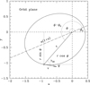 |
Fig. 1 Plane of the orbit. The axis x is defined by the intersection of the plane of the orbit and the plane of the sky. The periastron is at an angle φ0 from the x axis; φ is the angle between the x axis and the position on the orbit; ψ is the angle between the x axis and the velocity vector v. The angle between the position and velocity vectors is γ3D. |
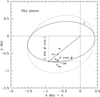 |
Fig. 2 Orbit projection on the sky. The angle between the position and velocity vectors on the sky is γ2D. |
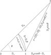 |
Fig. 3 Geometry of the binary system from the observer’s point of view. |
4.2 Distances and velocities
Figure 3 shows the geometric configuration of the binary system from the observer’s point of view, where we have assumed that star 1 (with mass M1) is at a distance D1 and star 2 (with mass M2) at a distance D2 with D1 < D2. For our sample of binaries the angle θ between the directions of the two stars of the pair is at most 5.4 arcmin, or 0.00157 radians, with a median value of 18.9 arcsec, or 10−4 radians (see Table B.3). This allows us to set the chord, S, to the length of the arc,  , and simplify the projected distance on the sky of the binary to
 (14)
(14)
and the true distance between the stars:
 (15)
(15)
The distances D1 and D2 follow approximately Gaussian distributions with means  pc and
  and dispersions
  and
and  , where p1 and p2 are the measured parallaxes and their respective errors δp1 and δp2 (see Table B.1). Then s and r are given by the Eqs. (14) and (15). We define Dmean = (D1 + D2)/2,
  and
and  . We compute
  inserting min(
 ) in Eq. (14) and r inserting
  and
and  in Eq. (15). We show in Sect. 5 that for our sample r overestimates r by more than one order of magnitude.
The relative velocities of the binary in the right ascension and declination directions are derived by scaling the proper motions of the pair (pmα1, pmδ1) and (pmα2, pmδ2) with the distances:
 (16)
(16)
 (17)
(17)
In analogy with what is written above, we defined  ,
,  ,
,  and
and  . Chae (2025, 2024) use
  and
and  in their analysis.
The errors on Vra and Vdec are in most of the cases less than 0.1%:
 (18)
(18)
 (19)
(19)
The relative velocity of the binary projected on the plane of the sky is:
 (20)
(20)
The angle between the vector connecting the pair and the vector of velocities on sky is:
 (21)
(21)
where (α1, δ1) and (α2, δ2) are the RA and Dec coordinates of the pair and δ = (δ1 + δ2)/2. Then, the components of Vtan parallel and orthogonal to the separation vector are
 (22)
(22)
We computed the errors δV||, δ V⊥, δVtan and δΓ2D by generating 100 Monte Carlo samples of Vra and Vdec and computing the RMS of the generated samples of V||, V⊥, Vtan and Γ2D. The errors reported in Table B.4 are on average 2% for Vra and Vdec. The error on the angle Γ2D is on average 0.3 degrees.
The (distance independent) component of the relative velocity of the binary along the line of sight is:
 (23)
(23)
with an error
 (24)
(24)
where δRV1 and δRV2 are the errors on the measured RVs and δVcor = 40 m s−1 takes into account the uncertainties in the gravitational redshift and convection motion corrections. On average, δVrad is on the order of 50 m s−1, except for the three pairs (#13, #15, #28) where no HARPS measurements for one of the binaries are available. Therefore, δVrad is one order of magnitude larger than δ Vtan.
We reversed the sign of the coordinate differences, Vrad, Vra, and Vdec if D1 > D2, which does not change the sign of Γ2D.
The total relative velocity of the binary is:
 (25)
(25)
from which we compute the ratio R = Vrad/Vtot. Its error δR is determined by generating 100 Monte Carlo samples of R and computing their RMS. Finally, the angle between the (tri-dimensional) vector connecting the pair and the vector of velocity difference is:
 (26)
(26)
where the + applies if D2 > D1 and the - if D2 < D1. We determined the error on Γ3D by generating 100 Monte Carlo samples of Γ3D and computing their RMS. Since δVtan is smaller than δVrad, the angle Γ2D is (much) better determined than Γ3D. Indeed, the error on the angle Γ3D is on average 4 degrees.
4.3 Best-fitting Newtonian solutions
Given the small errors affecting both measured velocities and masses of our WBs, we expect to reduce the uncertainty on the 3D separations of the binaries by searching for Newtonian orbits that reproduce the observed relative positions and velocities as much as possible. We sample the parameter space D1, D2, i, φ, e, φ0 to find the best matches between (Vrad, V∥, V⊥) and (vrad, v∥, v⊥) as follows. We start by sampling the distances D1 and D2 according to their Gaussian distributions set by the mean distances D1, D2 and errors δD1, δD2 derived from the parallaxes listed in Table B.1. We select (if they exist) the pairs of distances that deliver separations r that allow for maximum velocities  (see Eq. (3)) larger than the total velocity Vtot (see Eq. (25)), dropping picks with sin(arccos(s/r)) < Vrad/Vtot, since sin i ≥ Vrad/Vtot, see Eq. (7). The largest possible velocity is achieved for equal distances D = D1 = D2 and minimal separations rmin = s = Dθ. This sets the maximum allowed distance to:
 (27)
(27)
For a given Vtot and s, large values of r decrease s/r (increasing the minimal allowed inclination), require smaller values of r/a (pushing the phase towards pericenter), and/or larger values of eccentricity (see Eq. (3)).
We computed a combined distance figure of merit  , where
 (28)
(28)
and considered the separations ranked by  . We note that for the set of distances fulfilling this constraint and vmax ≥ V the resulting differences of Vtot are less than 10 m s−1 for the two branches of solutions D1 < D2 and vice versa. In contrast, the allowed variations in r are of the order of 50%, the ones in s a factor 10 less. The resulting allowed ratios s/r set the minimal allowed inclinations imin = arccos(s/r). We sampled the full range of allowed inclinations imin ≤ i ≤ π/2 with 1-3 degrees steps and determined the corresponding four allowed φ values using Eq. (6). The ratios Vtot/vmax deliver the values r/a = 2 - (Vtot/vN)2 (see Eq. (3)) that reproduce the measured total velocity exactly and in turn are linked to the 5/r ratios. From these r/a values we derived the minimum allowed eccentricity emin = |r/a - 1| (see Eq. (2)). We sampled the range of allowed eccentricities emin ≤ e ≤ 0.99 in 0.01 steps and computed the corresponding allowed values of cos(φ - φ0) through Eq. (1), each of which delivers two values for φ - φ0. For each of the allowed values of (i, φ, e, φ0), we computed vrad/v (see Eq. (7)) and γ2D (see Eq. (10)) and the quantities:
 (29)
(29)
We sorted the χ2 quantity:
 (30)
(30)
and we ranked the values of (i, φ, e, φ0) according to χ2. Finally, we selected the solutions that reproduce Γ3D best.
We show an example of the minimization algorithm for the binary HD 4552,BD+120090. Figure 4, left, presents the distribution of the best 100 distances with vmax/Vtot ≤ 1 ranked by  for the binary #1, HD 4552,BD+120090 in the D1, D2 plane. The allowed range of distances is narrow and translates into small (≈2 m s−1) variations of Vra, Vdec, and Vtan. The right plot shows the probabilities of the resulting best-fitting distances in 1D. The best fitting solution has distances very near the average distance of the pair and is bracket by the loci of the maximum separation
  allowed by the measured total WB velocity difference. Figure 5, left, shows that the separation, r, of the binary is up to a factor 3 larger than the separation, s, on the sky. The right plots shows that the value of r/a needed to reproduce the observed value of Vtot correlates with s/r. In turn, the best fitting values of s/r and r/a set the minimal allowed inclination and eccentricity (see Eqs. (5) and (2)).
Figure 6 illustrates how the orbit parameters i, φ, e, φ0 are constrained for each pair of distances selected in Fig. 5. The inclination is sampled starting from the minimal value set by s/r and delivers four possible values for φ (top left). The eccentricity is sampled starting from the minimal value set by r/a and delivers two values for φ - φ0 (top right). Each combination of i, φ and e, φ - φ0 is considered to achieve R = vrad/v (bottom left) and Γ2D = γ2D (bottom right) within the errors. The values of i, φ, e, φ - φ0 that deliver the first or, as in this case, second best of  , and Provide the value of γ3D nearest to Γ3D describe the best orbit reproducing the observations. In principle, Eq. (13) allows a direct determination of φ - φ0 as a function of e for a measured value of Γ3D. However, the larger observational errors affecting Γ3D make the focus on Γ2D preferable. In the end, the pair of distances D1 and D2 that deliver the optimal orbit have a
  value slightly larger (2.7) than the minimal one (2.5). Allowing a 2-3% increase in the total mass of the system is enough to decrease
  to less than 2.
We list the values of the best-fitting solutions in the Tables B.3, B.4, and B.5. The names of the binary pairs are listed in Table B.3. Together with their angular separation, the fitted distances D1 and D2, and X2D. Velocities Vra, Vdec, Vrad, Vtan, Vtot and angles Γ2D and Γ3D are given in Table B.4. The best-fitting quantities s, r, a, emin, e, imin, i, φ - φ0, φ0, ψ, γ2d, γ3d are listed in Table B.5, together with the period and acceleration of the orbit. These solutions are by no means unique: WBs with low values of  (roughly one third of the sample) can be fit with different combinations of distances. Given the relatively small size of our current sample, it goes beyond the scope of the paper to explore which (possibly non-Newtonian) solutions are also viable in these cases.
For the binary #24, HD 189739+HD189760, we cannot find any distance for which vmax ≥ Vtot. We report a solution obtained by increasing the total mass of the binary by 33%. Binary #24 not only requires this unrealistically large increase in mass, it also can be fit only by eccentricities almost equal to 1 and orbital periods as large as the age of the universe. We suspect that the system is not bound. The binary is marked in red in the following plots.
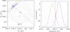 |
Fig. 4 Distances of the binary HD 4552,BD+120090. Left: contours of |


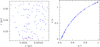 |
Fig. 5 Projected and intrinsic separations of the binary HD 4552,BD+120090. Left: the distribution of projected and intrinsic separations s and r. Right: r/a as a function of s/r. Red and blue crosses show D2 ≥ D1 and D2 < D1, respectively. The circled crosses show the best fitting solution. |
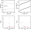 |
Fig. 6 Best-fitting Newtonian orbital solution for the binary HD 4552,BD+120090. Top left: the angle φ as a function of inclination. The red circle shows the selected value. Top right: the angle φ - φ0 as a function of eccentricity. The red circle shows the selected value. Bottom left: the black crosses show |


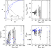 |
Fig. 7 Distances and separations of the WB sample. Top left: the histogram of |


5 Results
Figure 7 (top left) shows the histogram of  . Only seven pairs have
  > 2 and the distribution is more peaked at low
  values than the X2 distribution with 2 degrees of freedoms. There are no obvious correlations between
  and r, s/r and r/a. The top right plot shows that our mean distances Dmean agree within the errors with the Gaia mean distances. The bottom left plot shows that separations r directly inferred from Gaia distances increase with distance and overestimate the separations r derived by fitting the measured velocities by more than an order of magnitude. The bottom right plot shows that the WB separation projected on the sky, estimated by scaling the angular separation θ with the mean Gaia distance, increasingly overestimates s (obtained by scaling θ with the minimal Gaia distance), as the mean distance to the WB increases. Together with the trend of increasing r with Dmean and the large r̄/r ratio, this suggests that, dynamical studies of WBs samples with similar distance distributions and using deprojected s̄mean run the risk of systematically overestimating the true WB projected separation, therefore underestimating the acceleration and velocity of the system. This, in turn, could bias low the inferred accelerations and mimic a low-acceleration gravitational anomaly. The ratio s/s̄mean calculated with our best fitting distances is approximately equal to 1 up to the largest distances and separations.
Figure 8 shows the velocities Vra, Vdec, Vrad and Vtot as a function of the mean distance of the pair. Our current WB sample is clearly biased against large velocities at large distances. We compare our velocity differences Vtan and Vtot to the velocities differences  and
and  computed using mean Gaia distances in Fig. 9 (blue and red points), finding residuals less than 40 m s−1 and no systematic trends with distances. Differences between Vtan and Vtot (computed scaling the proper motions with the Gaia distances of each star separately) and
  and
and  are much larger, up to 200 m s−1, reflecting the uncertainties on the Gaia distances; still, no systematic trends with distances are observed.
The next two figures assess the quality of our best fit solutions. Fig. 10 shows that the ratio Vrad/Vtot, the angle Γ2D and the angle r3D are well reproduced within the errors. The residuals do not show trends with acceleration or separation r. Fig. 11 presents the same information in terms of velocity residuals, where we have added in quadrature an error equal to 3% of the model values to take into account the uncertainties on the total mass of the binaries. Without WB #24, radial, tangential and parallel velocities are reproduced with RMS of 21, 12 and 7 m s−1, respectively. Total velocities are reproduced exactly by construction. This investigation demonstrates that Newtonian solutions can be found down to the lowest accelerations probed by our (small) sample of WBs. Furthermore, Fig. 12 shows the histogram of the ratio  , where
  is the Newtonian circular velocity for the current projected separation. As expected, all WBs except binary #24 have
  and in qualitatively agreement with the Newtonian distributions of Pittordis & Sutherland (2018).
In the following we discuss how plausible these (non-unique) solutions are. The circled WBs in Fig. 10 show that some of the large separation, low-acceleration WBs have inclinations larger than 70°, or eccentricities larger than 0.8, or separations smaller than half the semimajor axis, or phases within 30° of the pericenter. A larger sample of WBs at large separations is needed to assess whether these possibly extreme properties persist.
Figure 13 shows the histograms of best-fitting eccentricities, inclination, phase angles φ - φ0, and semimajor orientation angles φ0. The eccentricity distribution is approximately thermal (f(e)de = 2ede), as expected for WB with separations larger than 1 kAU (Tokovinin 2020). The inclination distribution is peaked towards higher values, to some extent exceeding the expectations from a random distribution of inclinations (flat in cos i). Instead of the expected 15 ± 4 WBs with inclinations larger than 60°, we count 21 ±4 such systems, possibly still within the range allowed by low-number statistics. The phase distribution has the expected peak at apocenter and a suspicious second peak at pericenter exceeding expectations, but again with low number statistics. We computed the distribution of expected phases using Eq. (4), averaging over the best-fitting eccentricities. The orientation of the semimajor axis is approximately random, as expected.
Figure 14 shows how the ratios s/r, Vrad/Vtot and r/a constrain the inclination and eccentricity of the binaries. Two of the high eccentricity WBs are forced to have high inclinations (≥70°) by the required low values of s/r, further two by the large Vrad/Vtot ratio. WBs requiring low or high values of r/a are forced to have high eccentricities. Five of them have high inclinations, of which one is the possibly unbound pair #24. The measured angle r3D forces eight WBs to have large eccentricities (≥0.8), of which four have high inclination. Four of the WBs with phases near pericenter within 30° have the minimum inclination allowed by the Vrad/Vtot ratio.
Figure 15 investigates the role of the angle ψ to reproduce the ratio between the radial and tangential velocities (see Eq. (9)). The top panels show, as expected, that the ratio |Vrad|/Vtan is small for small eccentricities and inclinations and on average larger for large inclinations, with the largest values having also large eccentricities. The bottom panels show that low values of |Vrad|/Vtan at high eccentricities and inclinations are due to low values of |ψ|.
Figure 16 show correlations with Γ2D and Γ3D. As expected, both angles are ≈90 degrees at lowish inclinations and eccentricities. Consistently, the sky position and velocity vectors tend to be parallel or anti-parallel at high inclinations and high eccentricities. While no obvious trend between Γ2D with φ - φ0 appears (bottom left of Fig. 16), the expected modulation (see Eq. (13)) of Γ3D with φ - φ0, scaled by the eccentricity value, is clearly seen in the bottom right plot.
Finally, we summarize further (absence of) trends with eccentricities, inclinations, orbital phases, semimajor position angles and separations. There is a lack of eccentricities larger than 0.6 with inclinations lower than 45 degrees. There is a lack of low eccentricities at large separations, and a lack of high eccentricities at smaller separations, in line with the tendency discussed by El-Badry et al. (2021) of WBs having larger e at larger separations. There are no obvious correlations between eccentricity or inclination and phase φ - φ0 or semimajor axis position φ.
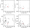 |
Fig. 8 Velocity differences of the WBs. As a function of the mean distance of the pair, we show Vra (top left), Vdec (top right), Vrad (bottom left) and Vtot (bottom right). |
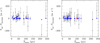 |
Fig. 9 Influence of velocity distance scaling. The blue and red points show the differences between the best fitting Vtan (left) and Vtot (right) and Vtan,mean and Vtot,mean (computed by scaling the proper motions with the mean Gaia distances Dmean) as a function of Dmean. The crosses show the differences between Vtan and Vtot (computed by scaling the proper motions with the Gaia distances of each star separately) and Vtan,mean and Vtot,mean. No systematic trends with distances are observed. |
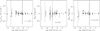 |
Fig. 10 Residuals ΔVrad/Vtot (left), ΔΓ2D (middle), and ΔΓ3D) (right) as a function of acceleration. We circle WBs with inclinations larger than 70° in the left, WBs with eccentricities larger than 0.8 in the middle, and WBs with r/a < 0.5 in the right plot. |
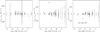 |
Fig. 11 Residuals Vrad - vrad (left), Vtan - vtan (middle), and Vk - vk (right) as a function of acceleration. |
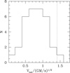 |
Fig. 12 Histogram of the ratio V = Vtot/Vcirc,s; except for WB #24, V is always less than |

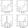 |
Fig. 13 Distributions of best-fitting parameters. The histogram of bestfitting eccentricities (top left), of inclinations (top right), of phases φ -φ0 (bottom left), and of orientation angles φ0 (bottom right) with the expected distributions (black lines). |
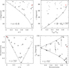 |
Fig. 14 Top left: inclination as a function of s/r. The line shows the minimum allowed inclination. The circled WBs have eccentricities larger than 0.8. Top right: inclination as a function of Vrad/Vtot. The line shows the minimum allowed inclination. The circled WBs have phases near the pericenter within 30°. Bottom left: eccentricity as function of r/a. The line shows the minimum allowed eccentricity. The circled WBs have inclinations larger than 70°. Bottom right: angle Γ3D as a function of eccentricity. The lines show the allowed angle range. The circled WBs have inclinations larger than 70°. |
6 Conclusions
In this work we have introduced two main novelties: the use of accurate radial velocities and the exploitation of the distance distribution provided by the Gaia parallaxes. With these, we are able to constrain the orbits of the WBs to test Einstein-Newton gravity in the low potential regime. We searched for archival data of WB candidates observed with the high precision spectrograph HARPS, finding 44 systems.
Precise RVs, repeated in time, allow one to single out and remove multiple systems, and high resolution observations deliver precise chemical abundances and stellar parameters. After cleaning, 32 out of the initial 44 systems (73%) survive our conservative selection criteria and these systems are suitable for testing Einstein-Newton law. The final sample has a median RUWE of 0.975 (with a highest value of 1.24) and a RV median variability of 10±6 ms−1. The star with the highest RV variability (29 m s−1), is known to host a massive exoplanet.
We obtained for each star an accurate RV, correcting the precise HARPS shifts for gravitational redshift and for convective motions in the stellar atmospheres using 3D model atmospheres. The corrected velocities are accurate to better than 40 m s−1. The comparison with Gaia shows a remarkable agreement in the RV zero point (67 m s−1) with a spread of 311 m s−1.
We exploited the distance distributions provided by the Gaia parallaxes to probe projected and tri-dimensional separations and velocity differences. In 31 of the 32 WBs at least one Newtonian orbit solution is possible with distances compatible with the Gaia parallax errors, the precision of the total mass estimates and the small velocity errors. For these 31 WBs we obtained reasonable orbit parameters, with some systems possibly too near pericenter and/or at too high inclination. We suspect that the remaining WB, #24, is not bound.
Chae (2024, 2025) finds a remarkable difference between WBs with separations larger than ~2 kAU (0.01 pc), and the closer systems, with the widely separated WBs breaking Newton law. We do not detect such a trend with our WB sample, much smaller in size but with higher precision radial velocities. To check whether this conclusion is statistically robust, we are in the process of collecting similarly good RVs for a large sample of WBs, to not only confirm the existence of Newtonian solutions in all cases, but also to verify the distributions of the retrieved orbital parameters are physically acceptable.
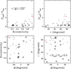 |
Fig. 15 Correlations with |Vrad|/Vtan (top) and |ψ| (bottom): eccentricity (left panels) and inclination (right panels). Circled crosses in the top panels show binaries with |ψ| < 20°; circled crosses in the bottom panels show binaries with |Vrad|/Vtan < 0.5. |
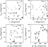 |
Fig. 16 Correlations with Γ2D (left) and Γ3D (right). The top plots show both angles as a function of inclination, circled WBs have eccentricities larger than 0.8. The bottom plots show both angles as function of orbit phase, circled WBs have inclinations larger than 70°. |
Acknowledgements
We thank the referee Charalambos Pittordis for a constructive report that helped us improving the presentation of our results. M.T.M. acknowledges the support of the Australian Research Council through Future Fellowship grant FT180100194. Research activities of the Board of Observational and Instrumental Astronomy (NAOS), at the Federal University of Rio Grande do Norte, are supported by continuous grants from the Brazilian funding agency Conselho Nacional de Desenvolvimento Científico (CNPq). I.C.L. (grant No. 313103/ 2022-4), and J.R.M. (grant No. 308928/20199) acknowledge CNPq research fellowships. This work has made use of data from the European Space Agency (ESA) mission Gaia (https://www.cosmos.esa.int/gaia), processed by the Gaia Data Processing and Analysis Consortium (DPAC, https://www.cosmos.esa.int/web/gaia/dpac/consortium). Funding for the DPAC has been provided by national institutions, in particular the institutions participating in the Gaia Multilateral Agreement.
Appendix A Systems discarded from the original sample
Out of the 44 initial systems with HARPS RVs, 12 have been discarded as unsuitable for the present study. We provide the interested reader with the justification of our choice.
HD20430 and HD20439: Our analysis provides an age of −700 Myrs. These stars belong to the Hyades cluster and may just be a proper motion pair.
HD13904 and BD10303B: The last observations in the catalog of both stars give a difference of −0.6 km s−1 with respect to the previous observations. The observations have been rereduced and the change in radial velocity confirmed. This seems a quadruple system. HD13904 has a RUWE larger than 2.
HD11790: RV varies of 500 m s−1 in a few days, the star has a companion.
CD-261686 and CD-2616866B: There is some confusion amongst the two target in the HARPS observations, and a difference between them of 3.7 km s−1 in radial velocity, that is in sharp disagreement with the RV difference measured by Gaia for these stars. Such a large RV difference is not compatible with a bound binary and the disagreement with Gaia suggests that the system is multiple.
HIP34407 and HD54100: Spina et al. (2021) report a difference of 0.15 dex in the [Fe/H] of the two stars. Ramírez et al. (2019) notice a spread of 60 m s−1 in radial velocity in their observations, indicating a possible companion. HARPS spectra (5 and 2 observations respectively) do not show high RV spread.
HD18142 and HD181544: HD 181544 shows a 30 m s−1 variability on 7 exposures, that is higher than average, and has a RUWE of 1.64.
HD2567 and HD2638: Many good HARPS observations are available. HD2638 has a high RV variability (47 m s−1) but is known to host a Jupiter-planet (Moutou et al. 2005). However, the system is triple, with an M star close to HD2638 (Wittrock et al. 2016), so not suitable for the test.
HD169392A and B: HD169392A has a RUWE of 4.2.
HD182817 and HD182797: HD182817 has a RUWE of 1.6 and a RV variability of 35 m s−1 .
HD116920 and HD116858: HD116920 has a RV variability of 111 m s−1.
Appendix B Tables
Gaia parameters of the 64 WB stars.
Stellar parameters and radial velocities of the 64 WB stars. The gravity values given in italics are Gaia values.
Angular separations, masses and recovered distances of the 32 WBs.
Measured velocities and angles of the 32 WBs.
Orbit-based parameters of the 32 WBs.
References
- Banik, I., Pittordis, C., Sutherland, W., et al. 2024, MNRAS, 527, 4573 [Google Scholar]
- Barbieri, M. 2024, https://doi.eso.org/10.18727/archive/3 [Google Scholar]
- Belokurov, V., Penoyre, Z., Oh, S., et al. 2020, MNRAS, 496, 1922 [Google Scholar]
- Bouchy, F., Pepe, F., & Queloz, D. 2001, A&A, 374, 733 [NASA ADS] [CrossRef] [EDP Sciences] [Google Scholar]
- Bressan, A., Marigo, P., Girardi, L., et al. 2012, MNRAS, 427, 127 [NASA ADS] [CrossRef] [Google Scholar]
- Chae, K.-H. 2023, ApJ, 952, 128 [NASA ADS] [CrossRef] [Google Scholar]
- Chae, K.-H. 2024, ApJ, 960, 114 [NASA ADS] [CrossRef] [Google Scholar]
- Chae, K.-H. 2025, arXiv e-prints [arXiv:2502.09373] [Google Scholar]
- Clarke, C. J. 2020, MNRAS, 491, L72 [Google Scholar]
- da Silva, L., Girardi, L., Pasquini, L., et al. 2006, A&A, 458, 609 [NASA ADS] [CrossRef] [EDP Sciences] [Google Scholar]
- El-Badry, K., Rix, H.-W., & Heintz, T. M. 2021, MNRAS, 506, 2269 [NASA ADS] [CrossRef] [Google Scholar]
- Haywood, R. D., Collier Cameron, A., Unruh, Y. C., et al. 2016, MNRAS, 457, 3637 [Google Scholar]
- Hernandez, X., Jiménez, M. A., & Allen, C. 2012, J. Phys. Conf. Ser., 405, 012018 [Google Scholar]
- Hernandez, X., Cookson, S., & Cortés, R. A. M. 2022, MNRAS, 509, 2304 [NASA ADS] [Google Scholar]
- Hernandez, X., Chae, K.-H., & Aguayo-Ortiz, A. 2024, MNRAS, 533, 729 [Google Scholar]
- Hwang, H.-C., Ting, Y.-S., & Zakamska, N. L. 2022, MNRAS, 512, 3383 [NASA ADS] [CrossRef] [Google Scholar]
- Jiang, Y.-F., & Tremaine, S. 2010, MNRAS, 401, 977 [Google Scholar]
- Katz, D., Sartoretti, P., Guerrier, A., et al. 2023, A&A, 674, A5 [NASA ADS] [CrossRef] [EDP Sciences] [Google Scholar]
- Kervella, P., Thévenin, F., & Lovis, C. 2017, A&A, 598, L7 [NASA ADS] [CrossRef] [EDP Sciences] [Google Scholar]
- Kervella, P., Arenou, F., & Thévenin, F. 2022, A&A, 657, A7 [NASA ADS] [CrossRef] [EDP Sciences] [Google Scholar]
- Lanza, A. F., Molaro, P., Monaco, L., & Haywood, R. D. 2016, A&A, 587, A103 [NASA ADS] [CrossRef] [EDP Sciences] [Google Scholar]
- Leäo, I. C., Pasquini, L., Ludwig, H.-G., & de Medeiros, J. R. 2019, MNRAS, 483, 5026 [Google Scholar]
- Lindegren, L., Hernández, J., Bombrun, A., et al. 2018, A&A, 616, A2 [NASA ADS] [CrossRef] [EDP Sciences] [Google Scholar]
- Lo Curto, G., Pepe, F., Avila, G., et al. 2015, The Messenger, 162, 9 [NASA ADS] [Google Scholar]
- Ludwig, H. G., Caffau, E., Steffen, M., et al. 2009, Mem. Soc. Astron. Italiana, 80, 711 [NASA ADS] [Google Scholar]
- Mayor, M., Pepe, F., Queloz, D., et al. 2003, The Messenger, 114, 20 [NASA ADS] [Google Scholar]
- Moutou, C., Mayor, M., Bouchy, F., et al. 2005, A&A, 439, 367 [NASA ADS] [CrossRef] [EDP Sciences] [Google Scholar]
- Pace, G., & Pasquini, L. 2004, A&A, 426, 1021 [NASA ADS] [CrossRef] [EDP Sciences] [Google Scholar]
- Penoyre, Z., Belokurov, V., & Evans, N. W. 2022a, MNRAS, 513, 2437 [NASA ADS] [CrossRef] [Google Scholar]
- Penoyre, Z., Belokurov, V., & Evans, N. W. 2022b, MNRAS, 513, 5270 [Google Scholar]
- Perdelwitz, V., Trifonov, T., Teklu, J. T., Sreenivas, K. R., & Tal-Or, L. 2024, A&A, 683, A125 [NASA ADS] [CrossRef] [EDP Sciences] [Google Scholar]
- Pittordis, C., & Sutherland, W. 2018, MNRAS, 480, 1778 [NASA ADS] [CrossRef] [Google Scholar]
- Pittordis, C., & Sutherland, W. 2019, MNRAS, 488, 4740 [NASA ADS] [CrossRef] [Google Scholar]
- Pittordis, C., & Sutherland, W. 2023, Open J. Astrophys., 6, 4 [Google Scholar]
- Ramírez, I., Khanal, S., Lichon, S. J., et al. 2019, MNRAS, 490, 2448 [CrossRef] [Google Scholar]
- Rodrigues, T. S., Girardi, L., Miglio, A., et al. 2014, MNRAS, 445, 2758 [Google Scholar]
- Rodrigues, T. S., Bossini, D., Miglio, A., et al. 2017, MNRAS, 467, 1433 [NASA ADS] [Google Scholar]
- Saar, S. H., & Donahue, R. A. 1997, ApJ, 485, 319 [Google Scholar]
- Spina, L., Sharma, P., Meléndez, J., et al. 2021, Nat. Astron., 5, 1163 [NASA ADS] [CrossRef] [Google Scholar]
- Tokovinin, A. 2020, MNRAS, 496, 987 [NASA ADS] [CrossRef] [Google Scholar]
- Wittrock, J. M., Kane, S. R., Horch, E. P., et al. 2016, AJ, 152, 149 [Google Scholar]
All Tables
Stellar parameters and radial velocities of the 64 WB stars. The gravity values given in italics are Gaia values.
All Figures
|
Fig. 1 Plane of the orbit. The axis x is defined by the intersection of the plane of the orbit and the plane of the sky. The periastron is at an angle φ0 from the x axis; φ is the angle between the x axis and the position on the orbit; ψ is the angle between the x axis and the velocity vector v. The angle between the position and velocity vectors is γ3D. |
| In the text | |
|
Fig. 2 Orbit projection on the sky. The angle between the position and velocity vectors on the sky is γ2D. |
| In the text | |
|
Fig. 3 Geometry of the binary system from the observer’s point of view. |
| In the text | |
|
Fig. 4 Distances of the binary HD 4552,BD+120090. Left: contours of |
| In the text | |
|
Fig. 5 Projected and intrinsic separations of the binary HD 4552,BD+120090. Left: the distribution of projected and intrinsic separations s and r. Right: r/a as a function of s/r. Red and blue crosses show D2 ≥ D1 and D2 < D1, respectively. The circled crosses show the best fitting solution. |
| In the text | |
|
Fig. 6 Best-fitting Newtonian orbital solution for the binary HD 4552,BD+120090. Top left: the angle φ as a function of inclination. The red circle shows the selected value. Top right: the angle φ - φ0 as a function of eccentricity. The red circle shows the selected value. Bottom left: the black crosses show |
| In the text | |
|
Fig. 7 Distances and separations of the WB sample. Top left: the histogram of |
| In the text | |
|
Fig. 8 Velocity differences of the WBs. As a function of the mean distance of the pair, we show Vra (top left), Vdec (top right), Vrad (bottom left) and Vtot (bottom right). |
| In the text | |
|
Fig. 9 Influence of velocity distance scaling. The blue and red points show the differences between the best fitting Vtan (left) and Vtot (right) and Vtan,mean and Vtot,mean (computed by scaling the proper motions with the mean Gaia distances Dmean) as a function of Dmean. The crosses show the differences between Vtan and Vtot (computed by scaling the proper motions with the Gaia distances of each star separately) and Vtan,mean and Vtot,mean. No systematic trends with distances are observed. |
| In the text | |
|
Fig. 10 Residuals ΔVrad/Vtot (left), ΔΓ2D (middle), and ΔΓ3D) (right) as a function of acceleration. We circle WBs with inclinations larger than 70° in the left, WBs with eccentricities larger than 0.8 in the middle, and WBs with r/a < 0.5 in the right plot. |
| In the text | |
|
Fig. 11 Residuals Vrad - vrad (left), Vtan - vtan (middle), and Vk - vk (right) as a function of acceleration. |
| In the text | |
|
Fig. 12 Histogram of the ratio V = Vtot/Vcirc,s; except for WB #24, V is always less than |
| In the text | |
|
Fig. 13 Distributions of best-fitting parameters. The histogram of bestfitting eccentricities (top left), of inclinations (top right), of phases φ -φ0 (bottom left), and of orientation angles φ0 (bottom right) with the expected distributions (black lines). |
| In the text | |
|
Fig. 14 Top left: inclination as a function of s/r. The line shows the minimum allowed inclination. The circled WBs have eccentricities larger than 0.8. Top right: inclination as a function of Vrad/Vtot. The line shows the minimum allowed inclination. The circled WBs have phases near the pericenter within 30°. Bottom left: eccentricity as function of r/a. The line shows the minimum allowed eccentricity. The circled WBs have inclinations larger than 70°. Bottom right: angle Γ3D as a function of eccentricity. The lines show the allowed angle range. The circled WBs have inclinations larger than 70°. |
| In the text | |
|
Fig. 15 Correlations with |Vrad|/Vtan (top) and |ψ| (bottom): eccentricity (left panels) and inclination (right panels). Circled crosses in the top panels show binaries with |ψ| < 20°; circled crosses in the bottom panels show binaries with |Vrad|/Vtan < 0.5. |
| In the text | |
|
Fig. 16 Correlations with Γ2D (left) and Γ3D (right). The top plots show both angles as a function of inclination, circled WBs have eccentricities larger than 0.8. The bottom plots show both angles as function of orbit phase, circled WBs have inclinations larger than 70°. |
| In the text | |
Current usage metrics show cumulative count of Article Views (full-text article views including HTML views, PDF and ePub downloads, according to the available data) and Abstracts Views on Vision4Press platform.
Data correspond to usage on the plateform after 2015. The current usage metrics is available 48-96 hours after online publication and is updated daily on week days.
Initial download of the metrics may take a while.