| Issue |
A&A
Volume 699, July 2025
|
|
|---|---|---|
| Article Number | A243 | |
| Number of page(s) | 11 | |
| Section | Extragalactic astronomy | |
| DOI | https://doi.org/10.1051/0004-6361/202554046 | |
| Published online | 09 July 2025 | |
CHANG-ES
XXXVI. The thin and thick radio discs
1
Hamburg University, Hamburger Sternwarte, Gojenbergsweg 112, 21029 Hamburg, Germany
2
Ruhr University Bochum, Faculty of Physics and Astronomy, Astronomical Institute (AIRUB), 44780 Bochum, Germany
3
Department of Physics and Astronomy, The University of Calgary, 2500 University Drive NW, Calgary AB T2N 1N4, Canada
4
Purple Mountain Observatory, Chinese Academy of Sciences, 10 Yuanhua Road, Nanjing 210023, China
5
Instituto de Astrofísica de Andalucía (IAA-CSIC), Glorieta de la Astronomía, 18008 Granada, Spain
6
Department of Physics, Engineering Physics, & Astronomy, Queens University, Kingston ON K7L 3N6, Canada
7
W.W. Hansen Experimental Physics Laboratory and Kavli Institute for Particle Astrophysics and Cosmology, Stanford University, Stanford, CA 94305, USA
⋆ Corresponding author: This email address is being protected from spambots. You need JavaScript enabled to view it.
Received:
5
February
2025
Accepted:
15
May
2025
Abstract
Context. Edge-on spiral galaxies give us an outsiders’ view of the radio halo that envelops these galaxies. Radio haloes are caused by extra-planar cosmic-ray electrons that emit synchrotron emission in magnetic fields.
Aims. We aim to study the origin of radio haloes around galaxies and infer the role of cosmic rays in supporting the gaseous discs. We test the influence of star formation as the main source of cosmic rays, as well as other fundamental galaxy properties such as mass and size.
Methods. We present a study of radio continuum scale heights in 22 nearby edge-on galaxies from the Continuum HAloes in Nearby Galaxies – an EVLA Survey (CHANG-ES). We employed deep observations with the Jansky Very Large Array in the S-band (2–4 GHz), imaging at 7″ angular resolution. We measured scale heights in three strips within the effective radio continuum radius, and corrected for the influence of angular resolution and inclination angle. We only included galaxies where a distinction between the two disc components can be made in at least one of the strips, which provided us with robust measurements of both scale heights.
Results. We find a strong positive correlation between the scale heights of the thin and thick discs and the star-forming radius, as well as star-formation rate (SFR); moderately strong correlations are found for the mass surface density and the ratio of SFR-to-mass surface density; no correlation is found with SFR surface density alone. Yet the SFR surface density plays a role as well: galaxies with high SFR surface densities have a rather roundish shape, whereas galaxies with little star formation only show a relatively small vertical extent in comparison to their size.
Conclusions. Thick gaseous discs are partially supported by cosmic-ray pressure. Our results are a useful benchmark for simulations of galaxy evolution that include cosmic rays.
Key words: cosmic rays / galaxies: fundamental parameters / galaxies: magnetic fields / galaxies: star formation / radio continuum: galaxies
Now at Deutsches Zentrum für Luft- und Raumfahrt e.V. (DLR), 53227 Bonn, Germany.
© The Authors 2025
 Open Access article, published by EDP Sciences, under the terms of the Creative Commons Attribution License (https://creativecommons.org/licenses/by/4.0), which permits unrestricted use, distribution, and reproduction in any medium, provided the original work is properly cited.
This article is published in open access under the Subscribe to Open model. This email address is being protected from spambots. You need JavaScript enabled to view it. to support open access publication.
1. Introduction
In the present Universe, disc galaxies consist of both a thin and a thick disc. The thin disc is composed of stars, dust, and gas with a scale height of a few hundred parsecs, respectively (Ferrière 2001). The thick disc comprises mostly ionised gas – in contrast to the thin disc where neutral and molecular components dominate, – cosmic rays and magnetic fields. While the thin disc is supported by the thermal pressure of the gas, the thick disc is inflated by non-thermal pressures (Cox 2005). The thick stellar disc has a different kinematic and chemical composition than the thin disc and thus can be used to constrain models for galaxy formation (Tsukui et al. 2025). The thick gaseous disc is the place where we can probe for outflows and inflows, and it therefore acts as an interface between the galaxy and the circumgalactic medium, which harbours a large reservoir of baryons surrounding galaxies (Tumlinson et al. 2017). In addition to the thin and thick discs, we note the existence of some more extended structures, such as the large-scale bubble discovered in the halo of NGC 4217 (Heesen et al. 2024a) and the extended radio blob around NGC 5775 (Li et al. 2008; Heald et al. 2022). It is unclear whether such large-scale radio features (>10 kpc) only exist in special cases, however, it is worth mentioning that there may be some more extended features beyond the thin and thick discs.
Observations of galaxies in the radio continuum allow us to study the distribution of cosmic rays and magnetic fields. Both are intertwined and oftentimes difficult to separate, yet synchrotron emission is one of the few avenues to study their influence on galaxy evolution. This is an ongoing research topic as comic rays follow magnetic field lines, and they are theorised to have a crucial effect on the efficiency of stellar feedback (Ruszkowski & Pfrommer 2023). This may be surprising as cosmic rays receive only 10% of the kinetic energy in the shock waves of supernova remnants, with the remainder thermalised to heat the gas, but there appears to be an increasing understanding of the theoretical underpinnings of winds that are driven by cosmic rays (Thompson & Heckman 2024). Cosmic rays are transported out of their sites of injection in star-forming regions, and thus establish a vertical pressure gradient. This gradient accelerates gas away from a galaxy without heating it (Salem & Bryan 2014).
One of the aims of the Continuum HAloes in Nearby Galaxies – an EVLA Survey (CHANG-ES) project was to investigate the workings of these processes by observational means (Irwin et al. 2012a, 2024a). CHANG-ES is a radio continuum survey of 35 nearby galaxies including L- (1–2 GHz) and C-band (4–6 GHz) data with full polarisation. CHANG-ES has so far delivered many insights into the structure and dynamics of the extra-planar interstellar medium. In combination with observations from the LOw Frequency ARray (LOFAR; van Haarlem et al. 2013), detailed observations of spectral ageing made it possible to study the transport of cosmic-ray electrons from the disc into the halo (Schmidt et al. 2019; Stein et al. 2019a, b, 2023; Miskolczi et al. 2019; Heald et al. 2022). These results were underpinned by a scale height analysis of the entire sample that showed that the escape of cosmic-ray electrons is possible, so that the galaxies are non-calorimetric (Krause et al. 2018). New insights into the magnetic field structure have also been gained. In NGC 4631, using Faraday rotation, magnetic ropes were revealed to be of kiloparsec size, with alternating magnetic field directions along the line of sight (Mora-Partiarroyo et al. 2019). In NGC 4666, a quadrupolar magnetic field structure was detected implying that there is a reversal of magnetic field direction across the plane of the disc (Stein et al. 2019a). Such a symmetry would be expected from the existence of a large-scale galactic dynamo operating at scales of tens of kiloparsecs, equivalent to the size of the galaxy. Henriksen & Irwin (2021) develop a theoretical basis for such large-scale field patterns. Finally, similar results were confirmed by a Faraday rotation study of the entire sample that shows the prevalence of X-shaped magnetic fields that are likely connected to galactic winds (Krause et al. 2020), with a corresponding study of the X-shaped magnetic field morphology presented in Stein et al. (2025).
With new S-band data, we are enriching the existing survey. With new deep polarimetric S-band (2–4 GHz) C-configuration observations, our aim is to cover a broad range of galaxy properties and strengthen the overall analysis. S-band polarised emission is the best probe for magnetic fields in the galaxies’ faint haloes, and the S-band is located in the crucial transition between Faraday-thin and -thick frequency regimes. While the CHANG-ES L-band data suffer from strong depolarisation and the C-band data have a limited resolution in Faraday space, our newly observed S-band data are essential and, in combination with the existing C- and L-band data, theyprovide new insights into the magnetic haloes of galaxies. Applying rotation measure synthesis to the combined data from the L, S, and C bands achieves an unprecedented resolution in Faraday space, and enable us to map the 3D structure of the ordered magnetic field. The results significantly improve our understanding of extended halo structures of a variety of magnetic field patterns in galaxies. Initial results are presented in Heesen et al. (2024a), Irwin et al. (2024b), and Xu et al. (2025) and show the versatility of the new S-band data.
In this new study, we revisit some of the work presented by Krause et al. (2018). They analyse the radio continuum scale height of the thick radio disc in both the L and C bands. While they modelled the vertical intensity distribution with two components, they did not include the analysis of the thin disc. We extend their work in two important ways. First, we include the analysis of the thin radio disc; second, we calculate deprojected mean intensities in both the thin and thick disc (Stein et al. 2019b, 2020). We use S-band data because of its superior angular resolution and sensitivity. A potential study of the integrated spectral behaviour of both disc components is deferred to a later work. In this work, we only use the total power radio continuum maps. We considered 22 galaxies from the CHANG-ES sample for analysis, the properties of which can be found in Table A.1. A full presentation of the data including polarisation will be presented in a forthcoming paper (Wiegert et al., in prep.).
This paper is organised as follows. Section 2 describes our sample selection, data reduction, and methodology. In Sect. 3 we present our resulting scale heights and flux densities, which we relate to fundamental galaxy parameters. We discuss our results in Sect. 4 before we conclude in Sect. 5. Appendix A contains more information about our galaxy sample and Appendix B presents our results in more detail.
2. Data and methodology
2.1. Observations
Observations were taken with the Jansky Very Large Array in the S-band in the frequency range of 2–4 GHz using full polarisation as part of observing programs 20A-018, 21A-033, and 22B-016 (PI: Y. Stein). We used the C configuration, which provides us with a nominal resolution of around 7″ using Brigg's robust weighting. The field of view as given by the diameter of the primary beam is 15′. The largest angular scale that we can image is  . Observations were taken in the standard fashion with 2048 channels of 100 kHz bandwidth each. We began with a scan of the primary calibrator used for flux scale and bandpass calibration. Our target observations were bracketed in scans of the secondary calibrator to determine the phase calibration.
2.2. Data reduction
We reduced our data with the Common Astronomy Software Applications (CASA; Team et al. 2022) version PIPELINE 6.4.12. For Stokes I, we used the ‘VLA calibration pipeline’ from the National Radio Astronomical Observatory without any further calibration or data flagging. The data were imaged with WSCLEAN version 2.9 using a multi-scale CLEAN algorithm (Offringa et al. 2014). The S-band data have a field of view of 15′, so that we have made maps with a size of two times the primary beam extent. For a few targets, we created larger maps in order to deconvolve confusing sources beyond a distance of one primary beam diameter. We then performed two rounds of self-calibration in phase only before creating final maps. For a few targets with strong residuals, we also performed one round of self-calibration in phase and amplitude. Also, for several sources we used mosaicked observations since they have a large apparent size. These are NGC 891, 3628, 4565, and 4631. In this case (with the exception of NGC 891, see below), we treated each of the two pointings separately and then combined them in a linear fashion using LINMOS within CASA.
We imaged and deconvolved maps using Brigg's robust weighting scheme with the robust parameter set to 0.5. Final maps were restored with Gaussian CLEAN beams using 7″ full width at half maximum (FWHM). We also applied the primary beam correction with WSCLEAN. Typical rms map noise values are between 3.5 and 5 μJy beam−1.
For NGC 891 we used joint deconvolution with TCLEAN as part of CASA. Two observations of NGC 891 were conducted in the S-band, each comprising two pointings. A single phase-only self-calibration loop was performed on the first observation, while two amplitude and phase self-calibration loops were applied to each observation. The data were manually flagged to remove any radio frequency interference (RFI). These data were imaged using the multi-scale TCLEAN algorithm, with the gridder parameter set to mosaic to account for the multiple pointings and Brigg's robust weighting of zero (robust = 0; Pourjafari et al. in prep.). The resulting map has an angular resolution of 5″, which we smoothed to a matching resolution.
2.3. Intensity profiles
We created vertical intensity profiles by averaging in boxes aligned in strips perpendicular to the major axis (see e.g. Krause et al. 2018, for details of this procedure). We used three strips with the middle one centred on the galaxy and the others symmetrically at larger galactocentric distances. For the width of the combined strips, we used the effective (e-folding) diameter in the radio continuum. We measured this by placing a 10″-wide strip centred on the major axis and fitting a Gaussian profile to the radio continuum emission. Hence, the width of each vertical strip is 2/3re, where re is the effective radius in the radio continuum. We then averaged intensities in boxes with the width equivalent to the strip width and with a height of approximately half the angular resolution. The height of each box was chosen at 3″. We created the intensity profiles using the NOD3 software package, where we made use of the BOXMODELS function (Müller et al. 2017).
In Fig. 1 we present the vertical intensity profiles in our galaxies in an example (mostly the middle) strip. In the linear–log xy diagram, an exponential function is a straight line. However, one can clearly see that more than one component is required because the slope of the profiles changes perceptively near the galactic mid-plane. In some cases, such as in NGC 891, a clear break is visible, in other cases the change is more gradual, such as in NGC 5775. This means we can observe both the thin and thick discs and we are able to separate them.
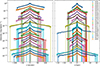 |
Fig. 1. Vertical radio continuum intensity profiles at 3 GHz in our sample galaxies. We show the intensities in the central strip of each galaxy, with the exception of NGC 3079, 4388, and 4666 where those in the eastern strip are shown. The left panel shows them as observed on the sky, whereas the right panel shows them projected to the assumed distance. Solid lines show two-component exponential model profiles deconvolved from the effective beam. The intensities were arbitrarily scaled in order to separate the profiles for improved display. |
We fitted exponential functions to the intensity profiles. Because of the limited angular resolution, the influence of the effective beam has to be taken into account. The effective beam is the superposition of the CLEAN beam (i.e. the intrinsic angular resolution) and the contribution from the inclined disc. Because our galaxies were not perfectly edge-on, the projected contribution from the radial profile along the minor axis needed to be considered. The resulting theoretical profiles were thus the convolution of the exponential distribution with a Gaussian function describing the effective beam, which can be described by an analytic formula (Dumke et al. 1995). For each galaxy, in Fig. 1 we show a model intensity profile for the two-component exponential distribution that is deconvolved from the effective beam. For our final results, we took the weighted mean of the amplitudes and scale heights of the thin and the thick discs in those strips where the reduced chi-squared value fulfilled  . In some cases, it was necessary to fit both haloes individually as the intensity profiles were asymmetric; in other cases, only one halo (either northern or southern) was fitted. The resulting amplitudes and scale heights of the thin and thick disc are presented in Table B.1.
To fit the intensity profiles with the two-component exponential profiles, NOD3 uses the SCIPY (Virtanen et al. 2020) CURVE_FIT implementation of the Levenberg–Marquardt algorithm and performs the uncertainty estimation for the fitting parameters based on the covariance matrix. Such an approach can lead to an underestimation of the parameter uncertainties, especially in the case of correlated parameters. Therefore, we refitted individual intensity profiles using a Markov chain Monte Carlo approach and found an overall agreement in the results. Based on these tests, we decided to use the fitting routine as implemented by NOD3.
2.4. Integrated intensity profiles
We integrated the intensities along the vertical direction in order to derive integrated flux densities (Stein et al. 2019a). These can be deprojected using the effective radius in radio continuum emission, so that we obtain a mean deprojected intensity as it would appear in a face-on galaxy. Hence
 (1)
(1)
where Ii is the deprojected mean intensity, wi is the amplitude in units of mJy beam−1, zi is the scale height in units of arcsec, and re is the effective radius in units of arcsec. Here, i∈{1,2} is for the thin and thick disc, respectively. The mean intensity of the combined thin and thick radio disc is then I=I1+I2.
2.5. Sample
The CHANG-ES sample consists of 35 galaxies. These were all included in the S-band survey with the exception of NGC 4244. In our analysis, we only included galaxies that allowed us to separate the thin and thick disc contributions. This was decided on the basis of the reduced chi-squared value  of the fitted intensity profiles. Only strips with
  were considered acceptable for the analysis. In those cases where a single component resulted in acceptable fits, we excluded the galaxy as the thin and thick discs could not be separated (NGC 3877, NGC 4192, UGC 10288). In some cases the projected disc was so prominent that no suitable profiles for fitting could be obtained (NGC 2613, 5297, 5792). Also, galaxies that only showed nuclear emission were omitted (NGC 2992, 4594, 4845, and 5084) as well as strongly interacting galaxies (NGC 660, 4438). This left us with a sample of 22 galaxies, the properties of which can be found in Table A.1.
Since our main results are based on the decomposition of the thin and thick disc components, we need to discuss a possible bias caused by the inclination correction. This could be particularly important for the thin disc component. This is because the selection of our sample is based on whether we can efficiently decompose these two components. We found no correlation between the inclination angle and scale height (ρs≤0.1). We chose the inclination angles adopted by Krause et al. (2018), or by Irwin et al. (2012a). The former ones were obtained from scale height fitting similar to ours, the later ones are from optical morphology. For an assumed inclination angle uncertainty of 5°, we estimate that the uncertainty of the thin disc is up to 50%, whereas that of the thick disc is less than 20%.
3. Results
3.1. Scale heights
First, we investigate the scale heights in both the thin and the thick discs. We find arithmetic mean scale heights of 0.45±0.06 and 1.47±0.20 kpc of the thin and thick disc (see Table B.1, for values), respectively. In Fig. 2 we show the dependence of scale height as a function of star-forming radius. We find significant correlations (p-value of p<0.05 from Spearman's test) between both thin and thick disc scale height and radius; both have moderate correlation strengths (Spearman's correlation coefficient of 0.3≤ρs≤0.6). Information about the best-fitting relation as shown in Fig. 2 and of those in the following figures is presented in Table 1. A related positive correlation of the thick disc scale height with the radio disc diameter was found by both Krause et al. (2018) and Galante et al. (2024). Figure 2 also shows that points above the best-fitting relation have predominantly high star-formation rate (SFR) surface densities, while for the ones below, the opposite is true. Hence, the size of the star-forming disc alone seems to be insufficient to determine the size of the radio halo, but a sufficient level of star formation may also be required.
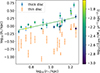 |
Fig. 2. Scale height as function of star-forming radius. For the thick disc, the best-fitting relation is shown. Data points for the thick disc are colour coded with the SFR surface density. |
Best-fitting relations using the equation log10(y) =alog10(x)+b with Spearman's rank correlation coefficient ρs.
Hence, we expect a combination of SFR surface density and radius, such as the SFR, to be important in determining the scale height. This is indeed the case we show in Fig. 3. Both for the thin and the thick disc, we found significant and strong positive correlations (p<0.05, ρs>0.6). Moreover, we investigated the dependence on SFR surface density alone. In this case, we find no significant correlation for the thick disc (p>0.1, ρs<0.3) and a moderate positive correlation for the thin disc. One reason may be that the influence of the star-forming radius is too large, as galaxies below the best-fitting relation have smaller radii, while the opposite holds for galaxies above the relation. A positive correlation with SFR surface density may be expected if the increased stellar feedback leads to outflows of cosmic rays and magnetic fields from the star-forming disc. If that is the case, then we also may expect to see a dependence on the mass surface density that governs gravitational attraction. In this case, we find evidence for a correlation (p<0.05), with a moderate negative correlation strength (−0.6≤ρs<−0.3). Assuming for a moment this correlation is real, and because the SFR and the mass surface densities are normalised with the same geometric area, we may consider simply the SFR-to-mass ratio instead. This quantity is related to specific SFR. However, because we use total instead of stellar mass, the concept is not quite applicable and we simply refer to the ratio instead. We find a significant moderate positive correlation between disc scale height and the ratio of SFR-to-mass surface density in both the thin and thick discs.
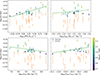 |
Fig. 3. Scale height in the thin and thick radio disc as function of various galaxy parameters. In each panel, we show the data points for the thick disc as filled circles colour coded with star-forming radius. Also, the best-fitting line for the thick disc is shown. The individual panels show the scale height as a function of SFR (top left), SFR surface density (top right), mass surface density (bottom left), and the ratio of SFR-to-mass surface density (bottom right). |
Hence, we conclude from this section that the SFR and the star-forming radius appear to be the prime parameters in determining the scale height of the radio discs. The negative correlation with the mass surface density and the positive correlation with the ratio of SFR-to-mass surface density are important, too, as secondary parameter. We also re-analysed the data in the L-band by Krause et al. (2018), who did not report a significant relation between thick disc scale height and SFR. We found that using the revised SFR values of Vargas et al. (2019) showed that only NGC 3003 is an outlier in the L-band data, whereas NGC 3735 (the galaxy with the second-lowest SFR surface density in Fig. 10 of Krause et al. 2018), lies on the best-fitting relation (the revised SFR value of NGC 3735 is a factor of three higher, see Vargas et al. 2019). Therefore, we found that the L-band data show a significant positive correlation with SFR, just as we found. However, due to the limited sample size, it was not quite so obvious visually when studying the relation. Therefore, it is understandable that Krause et al. (2018) did not report it.
3.2. Deprojected mean intensities
In this section, we present the relation between deprojected mean intensities and the SFR surface density. In Fig. 4 we show the intensities of the thin and thick radio discs, as well as their combination, as a function of the SFR surface density. All relations are significant (p-value < 0.05). However, whereas for the mean deprojected intensity of the thin disc and for the combined thin and thick disc we observe a strong correlation (ρs>0.7), the correlation for the thick radio disc is only moderate (ρs≈0.4). The relation in the thin disc is mildly super-linear with a slope of 1.20±0.30, whereas the combined relation has the expected nearly linear slope of 1.10±0.25. This slope is in good agreement with Li et al. (2016) who found a slope of 1.09±0.05 (as interpolated from their two frequencies) in the CHANG-ES sample for global measurements.
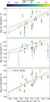 |
Fig. 4. Deprojected mean intensities as function of SFR surface density. Best-fitting relations are shown as solid lines, and the relation for integrated luminosities is shown as a dashed line (Li et al. 2016). We show the relation in the thin disc (top panel), thick disc (middle panel), and combined thin and thick discs (bottom panel). |
In Fig. 5 we show the ratio of the intensities of the thin to that of the thick disc as a function of the SFR surface density. We find no significant correlation (p>0.1). The mean ratio of thin-to-thick radio intensity is log10(I1/I2) = 0.01±0.54. Hence, on average the thin radio disc contributes only about the same to the deprojected mean intensity as the thick radio disc. This indicates that studies of face-on galaxies may suffer from a confusion of thin and thick disc, for instance when local correlations at kiloparsec scales are studied. In earlier works it was shown that this can be partially corrected when using the radio spectral index as a secondary parameter to correct for the effects of cosmic-ray transport (Heesen et al. 2024a).
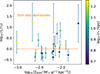 |
Fig. 5. Ratio of thin-to-thick disc deprojected intensities. Data points are shown as a function of SFR surface density and coloured according to their star-forming radius. The dashed line shows the boundary between thin disc-dominated (above line) and thick disc-dominated (below line) intensities. |
3.3. Normalised scale heights
The geometrical size of the galaxy is important as the cosmic-ray density decreases, both for diffusion and advection as a function of source distance. The scale size for normalisation depends on the size of the injection region. For this, we can use the star-formation distribution. Thus we use the effective radius as measured from the radio continuum image, to define the normalised scale height as
 (2)
(2)
where re is the effective radius of the radio continuum emission.
Figure 6 shows the normalised scale height as a function of the SFR surface density. We find significant correlations for both the thin and the thick radio disc. At high SFR surface densities, the scale height of the thin disc approaches a value of 0.5re. This means that the shape of the galaxy becomes rounder. At low SFR surface densities in contrast, the ratio of the scale height to the effective radius becomes as low as 0.1, hence the galaxy appears to be very thin in projection. We note that for energy equipartition between the cosmic rays and the magnetic field, the cosmic-ray scale height is approximately twice as high as the synchrotron scale height. Therefore, at high SFR surface densities, the cosmic-ray scale height approaches the effective radius of injection. This may give us some clues about the mode of cosmic-ray transport such as diffusion and advection.
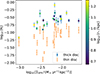 |
Fig. 6. Normalised scale heights as a function of SFR surface density. Data points of the thick radio disc are coloured according to the star-forming radius. |
4. Discussion
4.1. Hydrostatic equilibrium
Cox (2005) showed that cosmic rays are needed to explain the necessary pressure for a hydrostatic equilibrium in the Milky Way. Hence, we may assume
 (3)
(3)
where g is the gravitational acceleration, here assumed to be constant. We need an equation of state, such as B∝ρ0.5 (Heesen et al. 2023) to find for the magnetic pressure, and hence the cosmic-ray pressure, that PCR=const. ρ. The solution is an exponential decrease, PCR(z) =PCR,0exp(−z/hCR), with a cosmic-ray pressure scale height of
 (4)
(4)
We may express the gravitational acceleration via the mass surface density as g=π/(2G)Σtot, with G the gravitational constant. Hence, the scale height is proportional to the ratio of cosmic-ray pressure to density, and anti-proportional to the mass surface density. As cosmic rays are injected by star formation, a higher cosmic-ray pressure appears to be natural. Now the rate of star formation also depends on the gas density, but the slope is super-linear if the total gas density is considered (Kennicutt & Evans 2012). Hence, the ratio of cosmic-ray pressure to gas density would increase with SFR surface density. Combining these two relations, the hydrostatic equilibrium predicts that the cosmic-ray scale height should be proportional to the ratio of SFR to mass surface density (Eq. 4). This is indeed what we observe, and the relation is a significant one for the scale height (Sect. 3.1).
However, it is unclear if the thin disc actually is supported by the thermal pressure of the gas, while the thick disc is inflated by non-thermal pressures. There is yet little observational constraint about this. The pressure balance between different interstellar and circumgalactic medium phases was discussed in a few recent papers (Li et al. 2024b, a), following some simple early discussions in Wang et al. (2001) and Irwin et al. (2012b). The key conclusion is that the magnetic pressure and thermal pressure from hot gas reach a balance at a few kiloparsecs above the disc. Hence, cosmic-ray pressure is expected to inflate the thick disc only.
4.2. Relation of radio continuum to star formation
Our results for the different relations between radio continuum emission and star formation in thin and thick discs are an important test for the applicability of these relations. The global relation has a slope of close to one, when studied at gigaghertz frequencies (Li et al. 2016). At lower frequencies, we find a super-linear relation, which can be explained by the escaping of cosmic-ray electrons in smaller galaxies (Smith et al. 2021; Heesen et al. 2022). When studied at kiloparsec scales, the relation is sub-linear, which can be explained by cosmic-ray transport. Basically, there is an excess of cosmic-ray electrons in areas of less star formation due to diffusion (Heesen et al. 2023). This relation is close to linear at gigahertz frequencies, which is usually ascribed to the fact that electron calorimetry holds in galaxies.
Now, we showed that the relation is sub-linear for the thick disc component, but super-linear for the thin disc component. We can interpret this in such a way that the young cosmic-ray electrons in the disc have not yet diffused away and therefore the relation is close to linear, as also observed in face-on galaxies (Heesen et al. 2019, 2023). For older cosmic-ray electrons such as in the thick disc and in the inter-arm regions, the relation is sub-linear, again as we observe. Because of this trend, there is the tendency that galaxies with higher star-formation rate surface densities have a less prominent halo in comparison to the disc. What would be interesting for future studies is to take the spectral index distribution into account. Basically, we would expect the local relation to be different from linear, as it would be a large coincidence as this depends on the magnetic field strength as well (Werhahn et al. 2021). Thus, measurements of the radio spectral index could help to identify regions where spectral ageing and low-frequency absorption (Gajović et al. 2024) play a smaller role, so that we can measure the intrinsic relation unaffected by these effects.
As support for such future considerations, we also note that non-thermal emissions observed by the Fermi-LAT (Ackermann et al. 2012) also exhibit scaling with similar measures for SFR. Modelling of Milky Way-like galaxies viewed at high inclination angles (Porter et al., in prep.) indicates that quasi-linear correlation with the infrared and radio/γ-rays holds approximately for regions where there are significant fluxes of emissions. However, it departs significantly for sight lines that probe away from the geometrical thin extent of the disc. This is due to the production of non-thermal emissions throughout the extended halo region from the presence of both cosmic rays and target distributions (magnetic field, interstellar radiation field), whereas the infrared emissions only come from the narrow (when viewed close to edge-on) star-forming region. Unfortunately, for our sample of galaxies, their γ-ray emissions are too weak to be detected, and none appear as sources in the latest Fermi-LAT catalogue (4FGL-DR4; Ballet et al. 2023).
4.3. Cosmic-ray diffusion
Our findings of a positive correlation between scale height and galaxy size (Sect. 3.1) can be explained as follows: cosmic rays are injected in star-forming regions and are subsequently transported away, either by diffusion or advection, with the latter similar to streaming. In the case of diffusion, the steady-state solution is (Quataert et al. 2022)
 (5)
(5)
Here, r0 is the base radius, κ is the isotropic diffusion coefficient,  is the cosmic-ray energy injection per time, and r is the radius. We understood the base radius to be the size of the star-forming region that drives the vertical outflow. Therefore, we can associate the base radius with the effective radius of the radio continuum emission, re. Also, PCR,0 is the base cosmic-ray pressure at radius re. With a typical cosmic-ray injection of
  (Socrates et al. 2008), and a diffusion coefficient of 1028 cm2 s−1, we obtain
 (6)
(6)
where the pressure is in units of 10−12 erg cm−3, which we also assumed to be the base pressure. We assumed a SFR surface density of 10−2 M⊙ yr−1 kpc−2 and the radii are expressed in units of kiloparsecs. This can be approximated with an exponential function, where the cosmic-ray pressure scale height ≈re/4. This would then explain the observed positive correlation between the scale height of the thick disc and the star-forming radius.
5. Conclusions
We present a study of thin and thick radio discs in a sample of star-forming, late-type, edge-on galaxies. The thin disc is usually thought to be associated with the gaseous, star-forming disc, with a scale height of a few hundred parsecs, that contains stars, dust, and neutral atomic and molecular gas. The thick disc is associated with older stars, warm and hot ionised gas, and cosmic rays and magnetic fields. The thick disc might be the place where cosmic-ray-driven winds are launched (Girichidis et al. 2018), and where the mass exchange with the circumgalactic medium happens that is so crucial for understanding galaxy evolution (Tumlinson et al. 2017).
We used data from the CHANG-ES survey (Irwin et al. 2012a, 2024a) and exploit the new S-band (2–4 GHz) data with its superior sensitivity and angular resolution. We used a sample of 22 galaxies that fulfilled our selection criteria, in particular a clear detection of both the thin and thick disc. We also omitted galaxies that are AGN-dominated (Irwin et al. 2019) and those that are strongly interacting. We measured vertical intensity profiles in three strips centred on the minor axis, and accounted for the limited angular resolution and projection effects. These profiles were then fitted with two-component exponential functions to measure the scale height and deprojected mean intensities of both the thin and thick discs.
We find mean arithmetic scale heights of the thin and thick disc of 0.45±0.06 and 1.47±0.20 kpc, the latter value in agreement with (Krause et al. 2018). The thin disc scale height is in good agreement with the gaseous scale height of the warm neutral gas, whereas the thick disc corresponds to the warm ionised gas with a scale height in excess of 1 kpc (Lu et al. 2023). We found that the scale heights show a strong positive correlation with the star-forming radius, as was previously reported by Krause et al. (2018). Similarly, they show a moderate negative correlation with the mass surface density. We also explored the dependence on SFR surface density, but found no significant correlation for the thick disc. Again, both findings were already reported by Krause et al. (2018). As the size of the galaxy plays an important role, we then investigated the relation between scale height and the ratio of star-formation-to-mass surface density, which eliminates this dependence to some degree. We indeed found a moderate positive correlation. Such a relation can be explained if the thick disc is in hydrostatic equilibrium with a pressure contribution from cosmic rays (Sect. 4.1).
We then explored the relations between deprojected mean intensities and SFR surface density. We found that only the thin disc shows a strong correlation where the slope is in good agreement with a linear correlation as observed for the global relation at gigahertz frequencies. In contrast, the thick disc shows only a moderate correlation. The fact that the radio continuum emission is only weakly dependent on star formation can be explained by cosmic-ray transport. Since the halo contains mostly old cosmic rays, we no longer expect a strong correlation with the sites of cosmic-ray injection. These results are in good agreement with what is found in studies of edge-on galaxies at kiloparsec resolution where the star-forming areas show a linear relation, whereas the inter-arm areas show a sub-linear relation (e.g. Heesen et al. 2024b). When observing galaxies face-on, one needs to take the contribution from the halo into account, particularly when considering that on average the mean deprojected intensity of the thick disc is similar to that of the thin disc (Sect. 3.2).
Our results suggest that thick, gaseous discs are in hydrostatic equilibrium supported by cosmic-ray pressure (Boulares & Cox 1990; Cox 2005). Increasing the pressure-to-density ratio, such as is potentially expected in areas of higher SFR surface densities, leads to an inflated disc. On the contrary, higher mass surface densities lead to more compressed discs. Of course, a hydrostatic equilibrium does not apply globally. We also expect effects from cosmic-ray transport. Finally, we explored normalised scale heights, where we divided them by the effective radius as measured from radio continuum emission. We found a strong positive correlation between the normalised scale heights and the SFR surface density. However, we found no correlation between mass surface density or SFR-to-mass ratio. This suggests that galaxies with high SFR surface densities have a rather roundish shape, whereas galaxies with little star formation only have a relatively small vertical extent. Such a correlation can be explained by cosmic-ray transport, as the density scales with the size of the injection region and its relative distance to it (Sect. 4.3).
In the future, it would be worthwhile to extend this kind of study to other frequencies. This may shed some light on the question to what extent the age of the cosmic-ray electrons is different between thin and thick discs. This may then allow us to study the effects of cosmic-ray transport in a direct way.
Acknowledgments
We thank the anonymous referee for a concise and very helpful review. M.S. and R.-J. D. acknowledge funding from the German Science Foundation DFG, within the Collaborative Research Center SFB1491 “Cosmic Interacting Matters – From Source to Signal. MB acknowledges funding by the Deutsche Forschungsgemeinschaft (DFG) under Germany's Excellence Strategy – EXC 2121 “Quantum Universe” – 390833306 and the DFG Research Group “Relativistic Jets”. TW acknowledges financial support from the grant CEX2021-001131-S funded by MICIU/AEI/ 10.13039/501100011033, from the coordination of the participation in SKA-SPAIN, funded by the Ministry of Science, Innovation and Universities (MICIU). This research made use of following software packages and other resources: Aladin sky atlas developed at CDS, Strasbourg Observatory, France (Bonnarel et al. 2000; Boch & Fernique 2014); ASTROPY (Astropy Collaboration 2013, 2018); HyperLeda (http://leda.univ-lyon1.fr; Makarov et al. 2014); NASA/IPAC Extragalactic Database (NED), which is operated by the Jet Propulsion Laboratory, California Institute of Technology, under contract with the National Aeronautics and Space Administration; SAOImage DS9 (Joye & Mandel 2003); and SCIPY (https://scipy.org; Virtanen et al. 2020).
References
- Ackermann, M., Ajello, M., Allafort, A., et al. 2012, ApJ, 755, 164 [NASA ADS] [CrossRef] [Google Scholar]
- Astropy Collaboration (Robitaille, T. P., et al.) 2013, A&A, 558, A33 [NASA ADS] [CrossRef] [EDP Sciences] [Google Scholar]
- Astropy Collaboration (Price-Whelan, A. M., et al.) 2018, AJ, 156, 123 [Google Scholar]
- Ballet, J., Bruel, P., Burnett, T. H., Lott, B., & The Fermi-LAT Collaboration 2023, arXiv e-prints [arXiv:2307.12546] [Google Scholar]
- Boch, T., & Fernique, P. 2014, in Astronomical Data Analysis Software and Systems XXIII, eds. N. Manset, & P. Forshay, ASP Conf. Ser., 485, 277 [NASA ADS] [Google Scholar]
- Bonnarel, F., Fernique, P., Bienaymé, O., et al. 2000, A&AS, 143, 33 [NASA ADS] [CrossRef] [EDP Sciences] [Google Scholar]
- Boulares, A., & Cox, D. P. 1990, ApJ, 365, 544 [NASA ADS] [CrossRef] [Google Scholar]
- Cox, D. P. 2005, ARA&A, 43, 337 [Google Scholar]
- Dumke, M., Krause, M., Wielebinski, R., & Klein, U. 1995, A&A, 302, 691 [NASA ADS] [Google Scholar]
- Ferrière, K. M. 2001, Rev. Modern Phys., 73, 1031 [CrossRef] [Google Scholar]
- Gajović, L., Adebahr, B., Basu, A., et al. 2024, A&A, 689, A68 [NASA ADS] [CrossRef] [EDP Sciences] [Google Scholar]
- Galante, C. A., Saponara, J., Romero, G. E., & Benaglia, P. 2024, A&A, 685, A157 [NASA ADS] [CrossRef] [EDP Sciences] [Google Scholar]
- Girichidis, P., Naab, T., Hanasz, M., & Walch, S. 2018, MNRAS, 479, 3042 [NASA ADS] [CrossRef] [Google Scholar]
- Heald, G. H., Heesen, V., Sridhar, S. S., et al. 2022, MNRAS, 509, 658 [Google Scholar]
- Heesen, V., Buie, E. I., Huff, C. J., et al. 2019, A&A, 622, A8 [NASA ADS] [CrossRef] [EDP Sciences] [Google Scholar]
- Heesen, V., Staffehl, M., Basu, A., et al. 2022, A&A, 664, A83 [NASA ADS] [CrossRef] [EDP Sciences] [Google Scholar]
- Heesen, V., Klocke, T. L., Brüggen, M., et al. 2023, A&A, 669, A8 [NASA ADS] [CrossRef] [EDP Sciences] [Google Scholar]
- Heesen, V., Schulz, S., Brüggen, M., et al. 2024a, A&A, 682, A83 [NASA ADS] [CrossRef] [EDP Sciences] [Google Scholar]
- Heesen, V., Wiegert, T., Irwin, J., et al. 2024b, A&A, 691, A273 [NASA ADS] [CrossRef] [EDP Sciences] [Google Scholar]
- Henriksen, R. N., & Irwin, J. 2021, ApJ, 920, 133 [NASA ADS] [CrossRef] [Google Scholar]
- Irwin, J., Beck, R., Benjamin, R. A., et al. 2012a, AJ, 144, 43 [Google Scholar]
- Irwin, J., Beck, R., Benjamin, R. A., et al. 2012b, AJ, 144, 44 [NASA ADS] [CrossRef] [Google Scholar]
- Irwin, J., Wiegert, T., Merritt, A., et al. 2019, AJ, 158, 21 [NASA ADS] [CrossRef] [Google Scholar]
- Irwin, J., Beck, R., Cook, T., et al. 2024a, Galaxies, 12, 22 [NASA ADS] [CrossRef] [Google Scholar]
- Irwin, J., Cook, T., Stein, M., et al. 2024b, AJ, 168, 138 [NASA ADS] [CrossRef] [Google Scholar]
- Joye, W. A., & Mandel, E. 2003, in Astronomical Data Analysis Software and Systems XII, eds. H. E. Payne, R. I. Jedrzejewski, & R. N. Hook, ASP Conf. Ser., 295, 489 [NASA ADS] [Google Scholar]
- Kennicutt, R. C., & Evans, N. J. 2012, ARA&A, 50, 531 [NASA ADS] [CrossRef] [Google Scholar]
- Krause, M., Irwin, J., Wiegert, T., et al. 2018, A&A, 611, A72 [NASA ADS] [CrossRef] [EDP Sciences] [Google Scholar]
- Krause, M., Irwin, J., Schmidt, P., et al. 2020, A&A, 639, A112 [NASA ADS] [CrossRef] [EDP Sciences] [Google Scholar]
- Li, J. -T., Li, Z., Wang, Q. D., Irwin, J. A., & Rossa, J. 2008, MNRAS, 390, 59 [NASA ADS] [CrossRef] [Google Scholar]
- Li, J. -T., Beck, R., Dettmar, R. -J., et al. 2016, MNRAS, 456, 1723 [NASA ADS] [CrossRef] [Google Scholar]
- Li, J. -T., Lu, L. -Y., Qu, Z., et al. 2024a, ApJ, 967, 78 [NASA ADS] [CrossRef] [Google Scholar]
- Li, J. -T., Sun, W., Ji, L., & Yang, Y. 2024b, ApJ, 966, 239 [Google Scholar]
- Lu, L. -Y., Li, J. -T., Vargas, C. J., et al. 2023, MNRAS, 519, 6098 [NASA ADS] [CrossRef] [Google Scholar]
- Makarov, D., Prugniel, P., Terekhova, N., Courtois, H., & Vauglin, I. 2014, A&A, 570, A13 [NASA ADS] [CrossRef] [EDP Sciences] [Google Scholar]
- Miskolczi, A., Heesen, V., Horellou, C., et al. 2019, A&A, 622, A9 [NASA ADS] [CrossRef] [EDP Sciences] [Google Scholar]
- Mora-Partiarroyo, S. C., Krause, M., Basu, A., et al. 2019, A&A, 632, A10 [NASA ADS] [EDP Sciences] [Google Scholar]
- Müller, P., Krause, M., Beck, R., & Schmidt, P. 2017, A&A, 606, A41 [NASA ADS] [CrossRef] [EDP Sciences] [Google Scholar]
- Offringa, A. R., McKinley, B., Hurley-Walker, N., et al. 2014, MNRAS, 444, 606 [Google Scholar]
- Quataert, E., Thompson, T. A., & Jiang, Y. -F. 2022, MNRAS, 510, 1184 [Google Scholar]
- Ruszkowski, M., & Pfrommer, C. 2023, A&A Rev., 31, 4 [NASA ADS] [CrossRef] [Google Scholar]
- Salem, M., & Bryan, G. L. 2014, MNRAS, 437, 3312 [CrossRef] [Google Scholar]
- Schmidt, P., Krause, M., Heesen, V., et al. 2019, A&A, 632, A12 [NASA ADS] [EDP Sciences] [Google Scholar]
- Smith, D. J. B., Haskell, P., Gürkan, G., et al. 2021, A&A, 648, A6 [EDP Sciences] [Google Scholar]
- Socrates, A., Davis, S. W., & Ramirez-Ruiz, E. 2008, ApJ, 687, 202 [NASA ADS] [CrossRef] [Google Scholar]
- Stein, Y., Dettmar, R. J., Irwin, J., et al. 2019a, A&A, 623, A33 [NASA ADS] [CrossRef] [EDP Sciences] [Google Scholar]
- Stein, Y., Dettmar, R. J., Weżgowiec, M., et al. 2019b, A&A, 632, A13 [NASA ADS] [CrossRef] [EDP Sciences] [Google Scholar]
- Stein, Y., Dettmar, R. J., Beck, R., et al. 2020, A&A, 639, A111 [NASA ADS] [CrossRef] [EDP Sciences] [Google Scholar]
- Stein, M., Heesen, V., Dettmar, R. J., et al. 2023, A&A, 670, A158 [NASA ADS] [CrossRef] [EDP Sciences] [Google Scholar]
- Stein, M., Kleimann, J., Adebahr, B., et al. 2025, A&A, 696, A112 [NASA ADS] [CrossRef] [EDP Sciences] [Google Scholar]
- Team, T. C., Bean, B., Bhatnagar, S., et al. 2022, PASP, 134, 114501 [NASA ADS] [CrossRef] [Google Scholar]
- Thompson, T. A., & Heckman, T. M. 2024, ARA&A, 62, 529 [NASA ADS] [CrossRef] [Google Scholar]
- Tsukui, T., Wisnioski, E., Bland-Hawthorn, J., & Freeman, K. 2025, MNRAS, in press, [arXiv:2409.15909] [Google Scholar]
- Tumlinson, J., Peeples, M. S., & Werk, J. K. 2017, ARA&A, 55, 389 [Google Scholar]
- van Haarlem, M. P., Wise, M. W., Gunst, A. W., et al. 2013, A&A, 556, A2 [NASA ADS] [CrossRef] [EDP Sciences] [Google Scholar]
- Vargas, C. J., Walterbos, R. A. M., Rand, R. J., et al. 2019, ApJ, 881, 26 [NASA ADS] [CrossRef] [Google Scholar]
- Virtanen, P., Gommers, R., Oliphant, T. E., et al. 2020, Nat. Methods, 17, 261 [Google Scholar]
- Wang, Q. D., Immler, S., Walterbos, R., Lauroesch, J. T., & Breitschwerdt, D. 2001, ApJ, 555, L99 [NASA ADS] [CrossRef] [Google Scholar]
- Werhahn, M., Pfrommer, C., Girichidis, P., Puchwein, E., & Pakmor, R. 2021, MNRAS, 505, 3273 [NASA ADS] [CrossRef] [Google Scholar]
- Wiegert, T., Irwin, J., Miskolczi, A., et al. 2015, AJ, 150, 81 [Google Scholar]
- Xu, J., Yang, Y., Li, J. -T., et al. 2025, ApJ, 978, 5 [NASA ADS] [CrossRef] [Google Scholar]
Appendix A: Galaxy sample information
In Table A.1 we present some general information about our sample galaxies.
Properties of galaxies in the sample.
Appendix B: Observational results
In Table B.1 we present observational and derived results for our sample galaxies.
Scale heights and amplitudes of thin and thick radio discs; effective radii in the radio continuum.
All Tables
Best-fitting relations using the equation log10(y) =alog10(x)+b with Spearman's rank correlation coefficient ρs.
Scale heights and amplitudes of thin and thick radio discs; effective radii in the radio continuum.
All Figures
|
Fig. 1. Vertical radio continuum intensity profiles at 3 GHz in our sample galaxies. We show the intensities in the central strip of each galaxy, with the exception of NGC 3079, 4388, and 4666 where those in the eastern strip are shown. The left panel shows them as observed on the sky, whereas the right panel shows them projected to the assumed distance. Solid lines show two-component exponential model profiles deconvolved from the effective beam. The intensities were arbitrarily scaled in order to separate the profiles for improved display. |
| In the text | |
|
Fig. 2. Scale height as function of star-forming radius. For the thick disc, the best-fitting relation is shown. Data points for the thick disc are colour coded with the SFR surface density. |
| In the text | |
|
Fig. 3. Scale height in the thin and thick radio disc as function of various galaxy parameters. In each panel, we show the data points for the thick disc as filled circles colour coded with star-forming radius. Also, the best-fitting line for the thick disc is shown. The individual panels show the scale height as a function of SFR (top left), SFR surface density (top right), mass surface density (bottom left), and the ratio of SFR-to-mass surface density (bottom right). |
| In the text | |
|
Fig. 4. Deprojected mean intensities as function of SFR surface density. Best-fitting relations are shown as solid lines, and the relation for integrated luminosities is shown as a dashed line (Li et al. 2016). We show the relation in the thin disc (top panel), thick disc (middle panel), and combined thin and thick discs (bottom panel). |
| In the text | |
|
Fig. 5. Ratio of thin-to-thick disc deprojected intensities. Data points are shown as a function of SFR surface density and coloured according to their star-forming radius. The dashed line shows the boundary between thin disc-dominated (above line) and thick disc-dominated (below line) intensities. |
| In the text | |
|
Fig. 6. Normalised scale heights as a function of SFR surface density. Data points of the thick radio disc are coloured according to the star-forming radius. |
| In the text | |
Current usage metrics show cumulative count of Article Views (full-text article views including HTML views, PDF and ePub downloads, according to the available data) and Abstracts Views on Vision4Press platform.
Data correspond to usage on the plateform after 2015. The current usage metrics is available 48-96 hours after online publication and is updated daily on week days.
Initial download of the metrics may take a while.