| Issue |
A&A
Volume 699, July 2025
|
|
|---|---|---|
| Article Number | A234 | |
| Number of page(s) | 12 | |
| Section | Extragalactic astronomy | |
| DOI | https://doi.org/10.1051/0004-6361/202553817 | |
| Published online | 09 July 2025 | |
On the nature of buckling instability in galactic bars
Nicolaus Copernicus Astronomical Center, Polish Academy of Sciences, Bartycka 18, 00-716 Warsaw, Poland
⋆ Corresponding author: This email address is being protected from spambots. You need JavaScript enabled to view it.
Received:
20
January
2025
Accepted:
23
May
2025
Abstract
Many strong simulated galactic bars experience buckling instability, which manifests itself as a vertical distortion out of the disk plane, and later dissipates. Using a simulation of an isolated Milky Way-like galaxy, I demonstrate that the phenomenon can be divided into two distinct phases. In the first one, the distortion grows and its pattern speed remains equal to the pattern speed of the bar, so that the distortion remains stationary in the reference frame of the bar. The growth can be described with the mechanism of a driven harmonic oscillator with time-dependent force, which decreases the vertical frequencies of the stars. At the end of this phase, most bar-supporting orbits have banana-like shapes with a resonant vertical-to-horizontal frequency ratio close to two. The increase of amplitudes of vertical oscillations leads to the decrease of the amplitudes of horizontal oscillations and the shrinking of the bar. The mass redistribution causes the harmonic oscillators to respond adiabatically and increase the horizontal frequencies. In the following second phase of buckling, the pattern speed of the distortion increases – reaching one third of the circular frequency – but it decreases with radius. The distortion propagates as a kinematic bending wave and winds up, leaving behind a pronounced boxy/peanut shape. The increased horizontal frequencies cause the weakening of the bar and the transformation of banana-like orbits into pretzel-like ones, except in the outer part of the bar, where the banana-like orbits and the distortion survive. The results strongly suggest that the buckling of galactic bars is not related to the fire-hose instability, but it can be fully explained by the mechanism of vertical resonance creating the distortion that later winds up.
Key words: galaxies: evolution / galaxies: fundamental parameters / galaxies: kinematics and dynamics / galaxies: spiral / galaxies: structure
© The Authors 2025
 Open Access article, published by EDP Sciences, under the terms of the Creative Commons Attribution License (https://creativecommons.org/licenses/by/4.0), which permits unrestricted use, distribution, and reproduction in any medium, provided the original work is properly cited.
This article is published in open access under the Subscribe to Open model. This email address is being protected from spambots. You need JavaScript enabled to view it. to support open access publication.
1. Introduction
Many, perhaps even a majority, of late-type galaxies in the Universe possess an elongated structure in their inner parts, which is known as a bar. For about half a century we have known that galactic disks are generally unstable and form bars spontaneously (Hohl 1971; Ostriker & Peebles 1973), and this mechanism has been adopted as the main channel for the formation of bars. Another possibility, identified later on (Gerin et al. 1990; Noguchi 1996), involves interactions with other galaxies or bigger structures such as groups and clusters. Tidal forces naturally present during such encounters lead to the elongation of the stellar component and the formation of the bar if the circumstances of the interactions are favorable in terms of a small enough pericenter distance and prograde configuration (Łokas et al. 2014, 2016; Łokas 2018; Peschken & Łokas 2019). The formation and evolution of bars has been studied for decades using N-body simulations, and later on refinements such as the additional gas component and processes such as star formation and feedback. The dark-matter halo, originally introduced as a way to moderate the bar instability, has been shown to play a crucial role in bar formation due to its importance in the transfer of angular momentum (Athanassoula 2003).
The simulated bars, after a period of rapid growth, tend to become thicker later on, forming a bulge-like component with a boxy/peanut (BP) shape (Combes & Sanders 1981; Athanassoula 2005). This shape has been observed in many spiral galaxies viewed edge-on (Kruk et al. 2019), including our own Milky Way (Weiland et al. 1994; Ciambur et al. 2017). The thickening is often preceded by a short episode of vertical distortion or bending of the bar out of the disk plane; it was first described by Friedli et al. (1990), Pfenniger & Friedli (1991), and Raha et al. (1991) and is often referred to as buckling instability. However, it should be noted that the BP shape can also form without buckling (Combes et al. 1990; Pfenniger & Friedli 1991; Sellwood & Gerhard 2020; Li et al. 2023).
In addition to creating the BP shape, buckling also weakens the bar, but generally does not destroy it, and in most configurations it starts to regrow after the event. The instability may occur more than once in the lifetime of a bar, with the second episode usually lasting longer and happening in the outer parts (Martinez-Valpuesta et al. 2006; Kataria 2024). It has also been shown in idealized simulations that the presence of the gaseous component tends to suppress buckling (Debattista et al. 2006; Berentzen et al. 2007; Villa-Vargas et al. 2010; Athanassoula et al. 2013; Łokas 2020). However, more realistic configurations, modeled in cosmological simulations, do not seem to support this conclusion (Anderson et al. 2024). There is also no obvious correlation between the presence of a BP bulge, probably originating from buckling, and the global gas content in observed galaxies (Erwin & Debattista 2017).
Two hypotheses were proposed concerning the nature of buckling instability in galactic bars. Combes et al. (1990) and Pfenniger & Friedli (1991) suggested that the formation of the BP shape results from the trapping of typical orbits of the bar at vertical resonances. An alternative hypothesis for the origin of buckling involves the ratio of the vertical-to-horizontal velocity dispersion of the stars in the bar and relates it to the fire-hose instability known from plasma physics (Toomre 1966; Raha et al. 1991; Merritt & Sellwood 1994). In this picture, the instability is supposed to be triggered by a sufficiently low ratio of these dispersions (on the order of 0.3), which is characteristic of strong bars. Recently, the hypothesis based on vertical resonance seems to be getting more support from numerical studies (Li et al. 2023; McClure et al. 2025).
In this work, I revisited the issue of the origin and the nature of buckling instability in galactic bars using the insights from recently published works. The next section describes the recent progress that has been made in the field and how it can be used to build a convincing model of buckling instability. Sections 3 and 4 describe two phases of buckling into which the phenomenon can be divided, and Section 5 shows how the evolution of the orbital structure of the bar can be understood within this scenario. The discussion follows in Section 6.
2. Insights from recent studies
In Łokas (2019, hereafter L19), I studied buckling instability using a collisionless simulation of a Milky Way-like galaxy evolving in isolation. The galaxy N-body model was initiated with two components: a spherical dark-matter halo and an exponential disk, each containing 106 particles. The dark-matter halo had a Navarro-Frenk-White (Navarro et al. 1997) profile with a virial mass of MH = 1012 M⊙ and concentration of c = 25, while the exponential disk had a mass of MD = 4.5×10¹⁰ M⊙, scale-length of RD = 3 kpc, and thickness of zD = 0.42 kpc. The evolution of the galaxy was followed for 10 Gyr (with outputs saved every 0.05 Gyr) and revealed the bar to be forming rather slowly, reaching a maximum strength around t = 4.3 Gyr and the first buckling episode taking place at t = 4.5 Gyr. The reader is encouraged to browse this earlier paper (L19), because the results presented below refer to and build on previous findings.
As discussed in L19, in order to study the first buckling event in more detail, the simulation was rerun between t = 3.5 and t = 5.5 Gyr, saving outputs every 0.001 Gyr (2001 outputs in total), which allowed me to follow stellar orbits in sufficient detail to measure their properties. The properties of the orbits were estimated in the Cartesian reference frame of the bar with x, y, and z aligned with the major, intermediate, and minor axes of the bar. Then, I calculated the amplitudes of the stellar oscillations along the three axes, ax, ay, and az, and the frequencies of the orbits, fx, fy, and fz, using a discrete Fourier transform in two periods of 0.7 Gyr before and after buckling; that is, between 3.5 and 4.2 Gyr and between 4.8 and 5.5 Gyr, respectively. In the following, the quantities measured before buckling are denoted by symbols without primes, while those measured after buckling are denoted by the same symbols with primes; hence, fx and  will correspond to fx,before and fx,after used in L19, for example. The intermediate period, between 4.2 and 4.8 Gyr, was left out because at these times the orbits vary strongly, and the spectral analysis of stellar orbits is not reliable. It should be emphasized that the measurements of orbital properties were done “in vivo”, that is, in the live evolving bar rather than in a frozen potential, as is often done in the literature. Selecting bar-supporting orbits with ax<7 kpc (smaller than the length of the bar), ay<0.7ax (elongated along the bar), and those that underwent buckling – that is, those that increased their az amplitude during the evolution – gave a sample of almost 2×10⁵ orbits that were studied further.
The most important finding of that study was the discovery of a very tight linear relation between the orbital frequencies of the stellar orbits after buckling, which is very well fit (with the correlation coefficient of 0.99) by the relation  and can be approximated by the formula
 (1)
(1)
The parameter fp was identified numerically as the pattern speed of the bar, which did not vary strongly during buckling, and for this particular simulation it was equal to fp = 2.5 Gyr−1. It might be useful to note that in the more commonly used notation, with the circular frequency  and the vertical frequency
  , this relation translates to an even simpler formula: 3ν′ = 4Ω′. The relation, in terms of the 2D histogram of the distribution of the frequencies and the line given by Equation (1), is shown in the right panel of Fig. 1. Its origin is explored further below and in Section 4, where its connection to the pattern speed of the vertical distortion is described.
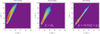 |
Fig. 1. 2D histograms of distribution of frequencies along the bar (fx) and along the vertical direction (fz) for bar-supporting stellar orbits that underwent buckling. The three panels from the left to the right show the distributions before buckling, during buckling, and after buckling, respectively. The white dashed lines and formulae indicate the approximate linear relations between the frequencies at the vertical resonance (middle panel) and after buckling (right panel). |
The existence of this very tight relation between the vertical and horizontal frequencies after buckling was later confirmed by Sellwood & Gerhard (2020), Li et al. (2023), and most recently by McClure et al. (2025) (for the case without the initial bulge), although they did not acknowledge the role of the pattern speed of the bar. However, using their published results concerning the appearance of the relation and the pattern speed of their simulated bars, one can easily demonstrate that the relation (1) is also obeyed by their results. It is especially noteworthy given that the pattern speeds of the bars are different in all these simulations. This confirms that the presence of the pattern speed in this relation is not just a numerical coincidence, it has a deeper meaning.
Comparing this relation with the much wider distribution of frequencies before buckling (left panel of Fig. 1), one can see that after buckling the relation becomes much tighter, and its slope changes significantly. While before buckling the distribution barely touches the fz = 2fx region (from above), after buckling all the stars are well below it. This strongly suggests that they must have crossed the vertical 2:1 resonance – that is, the fz = 2fx line – at a certain time. It is difficult to verify this using the spectral analysis of stellar orbits because the latter has to be performed on time spans containing many oscillations. Instead, Li et al. (2023) recently managed to determine the instantaneous frequencies of stellar orbits in their simulation of a buckling bar by measuring their periods directly. They confirmed that during buckling, the majority of stellar orbits in the bar indeed cross the 2:1 vertical resonance and thus provide strong arguments in favor of this mechanism as that responsible for triggering the vertical distortion.
Interestingly, plotting  (after buckling) as a function of fx (before buckling), one still obtains approximately the 2:1 resonance (middle panel of Fig. 1). This means that on the way to the resonance only fz changes, while fx remains approximately constant; if the resonance is present, even if fx is not yet changed it means that only the variation of fz is responsible for getting to the resonance. It does not mean that fx remains constant during the whole evolution, only that it changes mostly after the resonance is reached. This observation suggests a simple scenario, in which the buckling event can be divided into two distinct phases: the first one, where fz decreases while fx remains approximately constant; and the second one, where fx increases while fz remains unchanged. The next two sections describe the two phases in more detail.
Before moving on, it may be interesting to look at the evolution of the frequencies once again, but this time in the form of histograms of the ratio fz/fx, often discussed in similar studies (Portail et al. 2015). Figure 2 shows how the ratio evolved, from fz/fx>2 before buckling (blue), to  during buckling (green), and
  after buckling (red). I remind the reader that the green histogram shows a combination of the frequencies measured before buckling (fx) and after buckling (
 ), rather than real frequency estimates during buckling; however, the distribution, although rather wide, still peaks very close to the value of two expected for the vertical resonance.
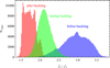 |
Fig. 2. Histograms of vertical-to-horizontal frequency ratios at different stages of evolution. The blue, green, and red distributions show the values of fz/fx>2 (before buckling), |


3. First phase: Growing the distortion
Figure 3 shows the distortion of the stellar component of the galaxy along the vertical direction (z) as it develops in the first stage of buckling. The maps in the subsequent panels show the mean position of the stars along z in different simulation outputs separated by 0.05 Gyr, starting with t = 4.1 Gyr. In the following panels, the distortion becomes more and more pronounced, preserving its shape with respect to the bar, which is oriented along the x-axis in all panels, until about t = 4.5 Gyr, after which time it starts to wind up.
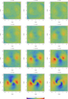 |
Fig. 3. Average position of stars along vertical direction at times t = 4.1 to 4.65 Gyr from the start of the simulation. Redder colors indicate the distortion above the disk plane, and the bluer ones show the distortion below it. The maps show the measurements in the reference frame of the bar, which is oriented along the x-axis. |
The initial stage of the formation of the distortion can be described using the Mathieu equation (Binney 1981). This formalism predicts instability of stellar orbits with resonant frequencies of fz = 2fx, which are thus able to increase their oscillations in the z direction. However, as can be seen from Fig. 1 (left panel) and Fig. 14 of L19 (middle left panel), the number of stars with such frequencies is very low before buckling. Although weakly populated, the resonance is by no means narrow, since the stars with resonant frequencies lie in a wide range of radii: between 0.5 and 4 kpc. The mechanism that is able to increase the number of such stars can be described in a simple way in terms of a driven harmonic oscillator.
I now suppose that some stellar orbits of the bar are caught at vertical resonance and that a small distortion out of the disk plane forms in the bar, such as the one shown in the upper left panel of Fig. 3. The other stars will feel a vertical force with a distribution tracing that of the existing distortion. The vertical resonance thus provides a seeding perturbation, which modifies the first orbits, and they change the mass distribution in the bar and its potential. The modified potential then changes the shape of subsequent orbits, which increase the overall distortion creating a kind of feedback loop. The picture involving the forced harmonic oscillator also helps us understand why one type of distortion (smile or frown) is selected and maintained. Once a small distortion appears due to the resonance, it builds up and enhances the same shape, because the force from the distorted mass distribution can only modify the orbits into this particular shape.
The vertical oscillations of the stars can therefore be described by the modified equation of the driven harmonic oscillator of the form
 (2)
(2)
where ω is the oscillation frequency of the star in the vertical direction, ωf is the frequency of the force, while F0 and α are constants. The classical term cos(ωft) describes the variability of the force due to the distortion of the mass distribution. The additional term (1−e−αt) represents its growth in time up to the maximum value, F0, with the growth rate controlled by α.
Let us express the vertical frequencies in terms of the horizontal frequencies, ω=fz/fx. As argued in the previous section, we can assume that the horizontal frequencies, fx, do not change in this stage of buckling. From the previous studies (L19), we know that before buckling, 2<fz/fx<4; the distribution of these frequency ratios is shown in Fig. 2 in the form of the blue histogram. Expressed in the same way, the force frequency ωf = 2.
The solution of Equation (2) with the natural choice of initial conditions z(0) =z0 and  can be found analytically with Mathematica software, but it is too complicated to cite it here in full. Instead, I discuss a few examples. The well-known outcome of the driven harmonic oscillator is to change the initial frequency, ω, to the frequency of the force, ωf, and it is also the case here. Figure 4 shows three representative orbits that illustrate this transformation. The upper panels of the figure present the solutions for z(t) for ω = 2.5, 3, and 3.5, which cover the range of interesting values of ω found to be present in the bar before buckling (Fig. 2). For all orbits, the values of the constants were assumed to be F0 = 10 and α = 0.1, which turn out to produce a sufficient effect.
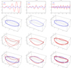 |
Fig. 4. Reaching resonance. The three columns show three examples of the evolution of stellar orbits under the growing force due to the distortion for different values of the initial frequency: ω = 2.5, 3, and 3.5. The solutions to Equation (2) were obtained with the force parameters F0 = 10 and α = 0.1 in all cases. The blue lines correspond to the initial oscillations and orbits, while the red lines show the modified ones. The panels of the upper row show the variation of the vertical position of the star along the orbit, while the next rows show the full orbits combining the motion along z with an ellipse in the xy plane without (blue, second row) and with (red, third row) the action of the force and the two combined (lower row). |
In each panel, the blue line corresponds to the initial (unforced) oscillation of the star z(t) =z0cos(ωt), and the red one to the solution under the effect of the force. One can see that the effect of the force is to increase the amplitude of the oscillation (from the initial small value of z0 = 0.5 kpc), but also to change its frequency. While within 4π the star oscillates five, six, and seven times for ω = 2.5, 3, and 3.5, respectively, before the forcing, it only oscillates four times after forcing. It should be noted that the orbits with initial frequencies differing more from the frequency of the force need more time to transform.
The lower panels of Fig. 4 show the corresponding 3D orbits of the stars in the form of the Lissajous curves combining the motion along z with the ellipse in the xy plane. The ellipses are the x1-type orbits, which are well known from classical studies of the orbital structure of bars (Contopoulos & Papayannopoulos 1980; Skokos et al. 2002). The blue and red orbits of the different columns show the 3D motion of the stars without and with the action of the force, and the three panels in the lowest row show them together for comparison. While the modified orbits are not exactly the banana-type orbits because of the variation of the amplitude, they are remarkably similar.
One can now imagine how the stellar orbits in the bar evolve in this phase of buckling. After a small perturbation out of the disk plane appears, the stars with ω only slightly larger than two will have their amplitudes strongly increased (left column of Fig. 4), thus increasing the force. This in turn will affect orbits with higher values of ω, bringing them all to ω∼2 (middle and right columns of Fig. 4). This is what we see in the first nine panels of Fig. 3: the distortion grows as more orbits join the resonance preserving its orientation with respect to the bar. This process takes about 0.4 Gyr (from t = 4.1 till t = 4.5 Gyr) in this simulation. At t = 4.5 Gyr, many of the stars that were on x1 orbits initially now follow the banana-like resonant orbits.
This simple description makes it possible to understand how the distortion can build up, creating orbits that are similar in shape to the well-known banana orbits. Such orbits would produce a distortion that is symmetrical with respect to the x-axis of the bar. As one can see from Fig. 3, this is not exactly the case. While the yellow and red part of the distortion, signifying departure above the disk plane, is approximately aligned with the bar ends, the blue part (below the plane) is not exactly perpendicular to the bar. This means that the average orbit of the stars at this stage looks more like the one shown in Fig. 5, which has its minima shifted with respect to the y-axis.
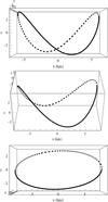 |
Fig. 5. Average orbit of stars at time of vertical resonance, in first stage of buckling, viewed along three directions: edge-on (upper panel), intermediate (middle panel), and face-on (lower panel). The dashed line indicates the more distant part of the orbit in the edge-on view. |
Interestingly, this kind of orbit also explains the mean velocity of stars during this phase of buckling discussed by Li et al. (2023). Figure 6 shows the mean velocity of the stars in the horizontal and vertical directions, vx and vz (upper and lower panels, respectively) at the time of maximum distortion (t = 4.5 Gyr). The motion of the stars can be understood if on average the stars follow the orbit shown in black. The components of the stellar motion (black arrows along the orbit) along the x and z directions agree with the overall average motion of all stars in these directions shown by the white arrows. This average orbit probably originates from the combination of banana and anti-banana (∞-like) orbits.
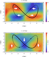 |
Fig. 6. Mean velocity of stars along x (upper panel) and along z (lower panel) in the bar at the time of maximum distortion, t = 4.5 Gyr, at the end of the first phase of buckling. The white arrows indicate the bulk motion of the stars in a given direction, and the small black arrows on the orbit (black line) indicate the direction of motion of the star along the orbit. |
The maximum distortion of the bar in the first phase of buckling, at time tb = 4.5 Gyr, can be approximated as zd(R,ϕ,tb) =z0(R)cos mϕ with m = 2. As discussed by Binney & Tremaine (2008) in the context of galactic warps (their Section 6.6.1), the evolution of such a distortion can be described as a propagation of a kinematic bending wave with a pattern speed of ωp=Ω−ν/2 (a different symbol, ωp, is used here to distinguish it from the pattern speed of the bar, Ωp, or fp in the notation of this paper). At resonance during buckling and using the notation adopted here,  , since
  at this time. This means that the bending wave propagates with the pattern speed of the bar, and therefore the distortion pattern seen in Fig. 3 remains stationary in the reference frame of the bar until tb = 4.5 Gyr. This is confirmed by the distribution of
  , which is plotted as a function of the amplitude of the oscillations along the horizontal axis, ax, in the left panel of Fig. 7. This combination of frequencies remains approximately constant with radius during buckling. Here, as before, it is assumed that the frequencies along the vertical direction have already changed (
 ), while those along the bar have not yet evolved (fx).
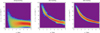 |
Fig. 7. Pattern speed of vertical distortion during and after buckling as function of amplitude of oscillations along the bar. The left panel shows the approximately constant pattern speed during buckling, assuming the evolved |


4. Second phase: Winding up the distortion
The evolution of the distortion in the vertical direction changes after tb = 4.5 Gyr. As demonstrated by the three panels of the lowest row in Fig. 3 (t = 4.55−4.65 Gyr), the pattern starts to wind up and continues to do so in the later stages illustrated in Fig. A.1 of the appendix. The passage of the bending wave at one particular distance from the center of the bar is visualized in Fig. 8, where the distortion of the bar is seen to evolve from smile-like to frown-like in the edge-on view. The same happens at all radii, but at a different rate, which leads to the more complicated distortion patterns seen at later times in Fig. A.1.
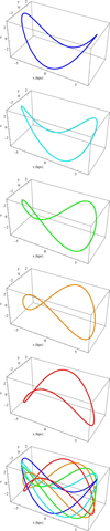 |
Fig. 8. Passage of bending wave. The images from top to bottom illustrate the evolution of the distortion in time at one selected distance from the center of the bar. As the minimum of the curve moves along the ellipse in the xy plane, the distortion changes from smile-like to frown-like in the edge-on view. The lowest image shows the combination of all the shapes. |
The connection between the passage of the bending wave and the distortion patterns is illustrated in Fig. 9 for t = 4.85 Gyr, one of the outputs shown in Fig. A.1. The maximum distortion was smile-like at all radii at tb = 4.5 Gyr. Between t = 4.5 and 4.85 Gyr, the bending wave rotated the distortion differently at different radii, and more so for those closer to the center (upper panel). This evolution creates a pattern of maxima and minima in the map of the average positions of the stars (middle panel) along the bar. The same pattern can also be discerned in the edge-on view of the surface density of the stellar component of the galaxy at this time (lower panel).
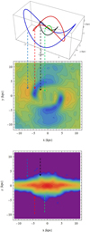 |
Fig. 9. Configuration leading to distortion seen in map of average positions of stars along vertical direction (middle panel) and in surface density of stellar component seen edge-on (along y, lower panel) for one selected time, t = 4.85 Gyr. The dashed arrows indicate the correspondence between the distortions rotated by the bending wave differently at different radii and the maxima and minima of the distributions of the stars in the face-on position map and edge-on density map. |
Figure A.1 shows that as the winding-up progresses, the pattern of maximal and minimal distortion moves outward toward the end of the bar but is still clearly visible, for example at t = 5.05 Gyr. Later on the distortion becomes so tightly wound that it ceases to be visible in the inner 5 kpc. The distortion, however, is still present at radii of R∼7 kpc, so in a sense buckling continues at these outer radii, as discussed below.
Thus, in the second phase of buckling the pattern speed of the bending wave is no longer constant with radius. Indeed, the middle panel of Fig. 7 shows that after buckling  decreases strongly as a function of
  (now all the quantities are primed and measured in the period of time after buckling, as discussed in Section 2). Interestingly, this combination of frequencies turns out to behave almost exactly the same way as
  (or Ω′/3 in the standard notation), which is shown in the right panel of Fig. 7. The only difference is that in the middle panel a small remnant of the constant pattern speed remains for
  . This corresponds to the small peak of the remaining resonant (banana) orbits with
  seen in the red histogram of Fig. 2. The equality between these two expressions,
  , immediately leads to Equation (1) after rearrangement of the terms.
It should be noted that a similar change in the behavior of  after buckling can also be seen in Fig. 13 of Li et al. (2023). After buckling (at t = 3.6 Gyr in their simulation) the same quantity, Ω−νz/2 in their notation (blue curve), increases and traces Ω (black curve) so that approximately Ω−νz/2=Ω/3, in agreement with the finding presented here.
The change in the behavior of the pattern speed of the bending wave after buckling can be traced to the change in the frequency along the bar, since this is the only quantity that varies from fx to  between the left and middle panels of Fig. 7. Indeed, by comparing fx(ax) before buckling with
  after buckling in Fig. 10, one can immediately see that the horizontal frequencies increase. This can be further appreciated in Fig. 11, which shows separately how the amplitude of the oscillations and the frequency evolved. This figure demonstrates that after buckling the amplitudes were on average decreased (
 ), while the frequencies were increased (
 ). The difference between the frequencies before and after buckling vanishes near the end of the bar at around R∼7 kpc. In this region,
  is still equal to the pattern speed of the bar fp because
  , and this is why the distortion survives.
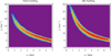 |
Fig. 10. Dependence of frequency of oscillations along bar on their amplitude before (left panel) and after (right panel) buckling. |
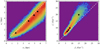 |
Fig. 11. Relations between amplitudes of oscillations along bar (left panel) and their frequencies (right panel) before and after buckling. White dashed lines indicate equality between the measured values and the black points mark the values corresponding to the first four orbits shown in Fig. 12, with properties listed in the first four rows of Table 1. |
5. Making pretzels from bananas
I now consider a few examples of horizontal frequencies of stellar orbits after buckling,  , from the range shown in the right panel of Fig. 10. The selected values are listed in the first column of Table 1. Using Equation (1), one can immediately find the corresponding vertical frequencies after buckling,
  . These values are given in the second column of the table, and their ratios,
  , are given in the third. The range of values of these ratios, which is between 1.5 and 2, covers the whole set seen in the red histogram in Fig. 2. Given that during buckling
  , one can immediately recover the initial horizontal frequencies, fx (fourth column). The typical amplitudes of the oscillations along the bar after and before buckling, giving an estimate of the size of the stellar orbits in this dimension,
  and ax, can then be found from fitting the very tight relations
  and fx(ax) in Fig. 10. Their values are given in the fifth and sixth columns of Table 1.
Properties of selected stellar orbits before and after buckling.
The passage of the bending wave may be interpreted as speeding up the motion of a star in the horizontal plane. For example (all frequencies in units of 1 Gyr−1), a star with fx = 7 made seven cycles in 1 Gyr, and after buckling it makes eight due to the bending wave:  ; a star with fx = 25/3 = 8.33 now has
  , while a star with fx = 15 makes five more cycles and has
  . These regularities can be generalized to
 (3)
(3)
with the values of ψ given in the penultimate column of Table 1. The dependence of ψ on the horizontal frequency can be approximated as
 (4)
(4)
where fp, as always, is the pattern speed of the bar. The formula makes the special significance of  clear, because ψ = 0 for this particular frequency. It means that the stellar orbits with frequencies equal to twice the pattern speed of the bar are not modified after buckling (last row of Table 1).
The transformation of other stellar orbits after buckling can be understood using 3D Lissajous curves. These curves can be parametrized as
![Mathematical equation: $$ (x, y, z) = [a \cos \phi , \ b \sin \phi , \ c \cos (m \phi + \phi _0)], $$](/articles/aa/full_html/2025/07/aa53817-25/aa53817-25-eq51.gif) (5)
(5)
where a,b,c are the amplitudes of the oscillations along x,y,z, respectively, and m is the ratio of the vertical and the horizontal frequency. It is assumed here that in the horizontal plane xy the orbits were, and remain, ellipses; that is, they originate from the x1 orbits. In this case, fy=fx before buckling and  after buckling. On the other hand, the ratio of the vertical and the horizontal frequency varies during buckling and changes from fz/fx>2 before the event to
  afterwards, as discussed above. For resonant orbits,
  , so a banana orbit is obtained for m = 2 in Equation (5). With the constant ϕ0 = 0, varying ϕ from 0 to 2π, we obtain the “pure” banana shown in the lower panel of Fig. 12. For this plot, it was assumed that
  kpc (in agreement with the values from Table 1 for
  Gyr−1) and b=c=a/2. Adopting a nonzero value of ϕ0 shifts the banana orbit toward an ∞-like orbit; for example, the orbit shown in Fig. 5 was obtained with ϕ0=−π/5.
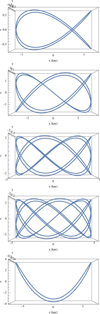 |
Fig. 12. Examples of pretzel orbits formed as result of buckling, viewed edge-on. The banana orbit is included in the lower panel. The frequency ratios of the orbits are |

At the end of the first phase of buckling, all orbits can be approximated as banana-like orbits with  . Using Equation (3), one obtains a relation between the frequencies after buckling:
 (6)
(6)
where n=(1+ψ)/(2ψ) and the values of the parameter n for the selected orbits are given in the last column of Table 1. In order to obtain the new orbits from the Lissajous curves given in the parametric form (5), one needs to replace m = 2, which is valid for the banana orbits, with (2−1/n). These values are obviously equal to the  ratios given in the third column of Table 1. The orbits obtained in this way using the Lissajous curves are shown in Fig. 12. The sizes of the orbits along x were adjusted to the values of
  from Table 1, while b=c=a/2 and ϕ0 = 0 were kept for all of them. It should be noted that in order to close, the orbits are required to cover 4π, 6π, 8π, and 10π in ϕ for n = 2, 3, 4, and 5, respectively.
The origin of these pretzel-like orbits can be understood by recalling that the bending wave speeds up the motion in the horizontal plane. I now focus on the first example of a fish-like orbit shown in the upper panel of Fig. 12. Starting at the upper right corner of the box, at the highest z position and following the orbit, one can see that in comparison with the original banana orbit (bottom panel) the star indeed reaches the next maximum of z not after half a cycle, but much further along the horizontal angle. Overall, the result is that the star makes only three full oscillations along z for each two oscillations in x, as expected from the frequency ratio for this orbit,  . Similar behavior is observed for the next orbits shown in Fig. 12, but to a lesser extent. The orbits with
  , 7/4, and 9/5 make five, seven, and nine oscillations in z for each three, four, and five oscillations in x, respectively. The limiting case of this sequence is obviously the banana orbit with
  , which remains unchanged.
The positions of the first four orbits from Table 1 and Fig. 12 in the  and
and  planes are shown as black dots in Fig. 11. The variation of these two quantities in the second phase of buckling suggests that they change adiabatically. As discussed in Section 3.6.2 of Binney & Tremaine (2008), the increase of the horizontal frequency of a harmonic oscillator by a factor (1+ψ) described by Equation (3) should correspond to the decrease of the amplitude of oscillations according to
  . The numerical values in Table 1 indeed obey these relations.
6. Discussion
In this work, I revisited the issue of the origin and interpretation of the buckling instability in galactic bars. It was proposed that the phenomenon can be divided into two distinct phases. The first one involves the growth of the distortion of the bar out of the disk plane due to the vertical resonance of stellar orbits in the bar. The growth of the distortion can be described with the mechanism of the driven harmonic oscillator where the initial small perturbation acts as a driving force and modifies the vertical frequencies of other orbits. The distortion retains its orientation with respect to the bar until reaching a maximum value.
The increase of the amplitudes of the oscillations of the stars in the vertical direction is accompanied by a decrease of the amplitudes along the bar and the bar shrinks leading to the increase of the mass in the central parts, as noticed by Li et al. (2023). The harmonic oscillators then seem to respond adiabatically, increasing the frequencies of the oscillations along the bar. Indeed, the factors by which the horizontal frequencies and amplitudes change agree with this interpretation.
As a result of the increased horizontal frequencies, in the second phase of buckling the pattern speed of the vertical distortion is no longer equal to the pattern speed of the bar – it is higher – and the distortion starts to wind up. The banana orbits that dominated the orbital structure of the bar at the time of the resonance evolve into pretzel-like orbits with vertical-to-horizontal frequency ratios below two. The winding up of the distortion also explains why the bar becomes weaker after buckling. Namely, the winding up is associated with faster rotation of the stars in the horizontal plane, which means that the orbits become less radial.
The equation of a driven harmonic oscillator (although without the force growing in time) was previously used in the context of bar buckling by Collier (2020) in an attempt to relate buckling to the phenomenon of Landau damping. Here, instead, this equation was used to demonstrate how the initial small deviation from the vertical symmetry can build up, leading to a strong global distortion of the bar, and the scenario bears no relation to Landau damping.
The violent buckling event seen in the simulation described here, leading to the strong changes in the orbital structure of the bar, seems to be characteristic of pure disks embedded in dark-matter halos, with no bulge component. In a recent study, McClure et al. (2025) looked into the phenomenon using simulations with different bulges of increasing mass. In the case without the bulge, their results are very similar to the ones discussed here; namely, after buckling the orbital frequencies display a very tight relation similar to the one shown in the right panel of Fig. 1. With increasing bulge mass, the resonant orbits still appear, but they do not evolve strongly toward vertical-to-horizontal frequency ratios below two, and they remain close to this resonant value. It seems, therefore, that the bulge does not inhibit the appearance of the vertical resonance, but it does prevent the passage to the second phase of buckling as described here. This is understandable given the importance of mass redistribution in changing the horizontal frequencies, mentioned above. With the additional massive component in the center, this must certainly look different.
Recently, Zozulia et al. (2024) studied the vertical evolution of a mature simulated bar, long after the violent buckling event. They reported behavior similar to that described here, namely the catching of the orbits at resonance and their later passage to vertical-to-horizontal frequency ratios below two, which they refer to as the “circulation mode”. This stage of bar evolution corresponds to the period after t = 5 Gyr in the simulation discussed here when the distortion is preserved only in the outer part of the bar (last panels of Fig. A.1). As discussed in L19, this distortion survives for a few gigayears, shifting toward the outer part of the bar and seeding the second episode of buckling later on. It therefore seems that as the bar grows, its outer parts continuously increase amplitudes of their oscillations in the vertical direction in a kind of quiescent buckling. The process described by Zozulia et al. (2024) is thus not essentially different from the violent buckling event studied here. The latter only happens on a shorter timescale and in the whole inner part of the bar. This picture of the moving distortion also agrees with the early results of Pfenniger & Friedli (1991), which found (their Fig. 14) that the position of the vertical resonance shifts to larger radii after the formation of the BP shape.
A few open questions remain concerning the analysis presented here. For example, it is still not clear why the pattern speed of the vertical distortion increases in such a particular way in the second stage of buckling and becomes equal to a third of the circular frequency. A related question concerns why the banana orbits in the outer part of the bar remain unchanged. This region is characterized by the horizontal frequency equal to twice the pattern speed of the bar, so the pattern speed of the vertical distortion remains equal to the pattern speed of the bar and the distortion does not wind up there.
In summary, this work demonstrates that the phenomenon of buckling instability is not related to the fire-hose instability known from plasma physics, but instead it is triggered by the vertical resonance of bar orbits. The resonance leads to the growing distortion of the bar, which later winds up, resulting in a transformation of banana-like orbits into pretzel-like ones and the formation of a BP shape.
Acknowledgments
I am grateful to the anonymous referee for useful comments. Computations for this work have been performed using the computer cluster at the Nicolaus Copernicus Astronomical Center of the Polish Academy of Sciences (CAMK PAN).
References
- Anderson, S. R., Gough-Kelly, S., Debattista, V. P., et al. 2024, MNRAS, 527, 2919 [Google Scholar]
- Athanassoula, E. 2003, MNRAS, 341, 1179 [Google Scholar]
- Athanassoula, E. 2005, MNRAS, 358, 1477 [NASA ADS] [CrossRef] [Google Scholar]
- Athanassoula, E., Machado, R. E. G., & Rodionov, S. A. 2013, MNRAS, 429, 1949 [Google Scholar]
- Berentzen, I., Shlosman, I., Martinez-Valpuesta, I., & Heller, C. H. 2007, ApJ, 666, 189 [Google Scholar]
- Binney, J. 1981, MNRAS, 196, 455 [NASA ADS] [Google Scholar]
- Binney, J., & Tremaine, S. 2008, Galactic Dynamics, 2nd edn. (Princeton: Princeton Univ. Press) [Google Scholar]
- Ciambur, B. C., Graham, A. W., & Bland-Hawthorn, J. 2017, MNRAS, 471, 3988 [NASA ADS] [CrossRef] [Google Scholar]
- Collier, A. 2020, MNRAS, 492, 2241 [Google Scholar]
- Combes, F., & Sanders, R. H. 1981, A&A, 96, 164 [NASA ADS] [Google Scholar]
- Combes, F., Debbasch, F., Friedli, D., & Pfenniger, D. 1990, A&A, 233, 82 [NASA ADS] [Google Scholar]
- Contopoulos, G., & Papayannopoulos, T. 1980, A&A, 92, 33 [NASA ADS] [Google Scholar]
- Debattista, V. P., Mayer, L., Carollo, C. M., et al. 2006, ApJ, 645, 209 [Google Scholar]
- Erwin, P., & Debattista, V. P. 2017, MNRAS, 468, 2058 [Google Scholar]
- Friedli, D., & Pfenniger, D. 1990, in Bulges of Galaxies, ESO Conference and Workshop Proceedings, eds. B. J. Jarvis, & D. M. Terndrup (Garching: ESO), 35, 265 [Google Scholar]
- Gerin, M., Combes, F., & Athanassoula, E. 1990, A&A, 230, 37 [NASA ADS] [Google Scholar]
- Hohl, F. 1971, ApJ, 168, 343 [NASA ADS] [CrossRef] [Google Scholar]
- Kataria, S. K. 2024, MNRAS, 534, 3565 [Google Scholar]
- Kruk, S., Erwin, P., Debattista, V. P., & Lintott, C. 2019, MNRAS, 490, 4721 [Google Scholar]
- Li, X., Shlosman, I., Pfenniger, D., & Heller, C. 2023, MNRAS, 520, 1243 [NASA ADS] [CrossRef] [Google Scholar]
- Łokas, E. L. 2018, ApJ, 857, 6 [Google Scholar]
- Łokas, E. L. 2019, A&A, 629, A52 [NASA ADS] [CrossRef] [EDP Sciences] [Google Scholar]
- Łokas, E. L. 2020, A&A, 634, A122 [NASA ADS] [CrossRef] [EDP Sciences] [Google Scholar]
- Łokas, E. L., Athanassoula, E., Debattista, V. P., et al. 2014, MNRAS, 445, 1339 [Google Scholar]
- Łokas, E. L., Ebrová, I., del Pino, A., et al. 2016, ApJ, 826, 227 [Google Scholar]
- Martinez-Valpuesta, I., Shlosman, I., & Heller, C. 2006, ApJ, 637, 214 [NASA ADS] [CrossRef] [Google Scholar]
- McClure, R. L., Beane, A., D’Onghia, E., Filion, C., & Daniel, K. J. 2025, MNRAS, 537, 1475 [Google Scholar]
- Merritt, D., & Sellwood, J. A. 1994, ApJ, 425, 551 [NASA ADS] [CrossRef] [Google Scholar]
- Navarro, J. F., Frenk, C. S., & White, S. D. M. 1997, ApJ, 490, 493 [Google Scholar]
- Noguchi, M. 1996, ApJ, 469, 605 [Google Scholar]
- Ostriker, J. P., & Peebles, P. J. E. 1973, ApJ, 186, 467 [Google Scholar]
- Peschken, N., & Łokas, E. L. 2019, MNRAS, 483, 2721 [Google Scholar]
- Pfenniger, D., & Friedli, D. 1991, A&A, 252, 75 [NASA ADS] [Google Scholar]
- Portail, M., Wegg, C., & Gerhard, O. 2015, MNRAS, 450, L66 [NASA ADS] [CrossRef] [Google Scholar]
- Raha, N., Sellwood, J. A., James, R. A., & Kahn, F. D. 1991, Nature, 352, 411 [Google Scholar]
- Sellwood, J. A., & Gerhard, O. 2020, MNRAS, 495, 3175 [Google Scholar]
- Skokos, Ch., Patsis, P. A., & Athanassoula, E. 2002, MNRAS, 333, 847 [Google Scholar]
- Toomre, A. 1966, Geophys. Fluid Dyn., 66–46, 111 [Google Scholar]
- Villa-Vargas, J., Shlosman, I., & Heller, C. 2010, ApJ, 719, 1470 [Google Scholar]
- Weiland, J. L., Arendt, R. G., Berriman, G. B., et al. 1994, ApJ, 425, L81 [NASA ADS] [CrossRef] [Google Scholar]
- Zozulia, V. D., Smirnov, A. A., Sotnikova, N. Ya., & Marchuk, A. A. 2024, A&A, 692, A145 [NASA ADS] [CrossRef] [EDP Sciences] [Google Scholar]
Appendix A: Later evolution of the distortion pattern
This appendix presents the continuation of Fig. 3 and shows the evolution of the vertical distortion pattern of the bar after it starts to wind up.
All Tables
All Figures
|
Fig. 1. 2D histograms of distribution of frequencies along the bar (fx) and along the vertical direction (fz) for bar-supporting stellar orbits that underwent buckling. The three panels from the left to the right show the distributions before buckling, during buckling, and after buckling, respectively. The white dashed lines and formulae indicate the approximate linear relations between the frequencies at the vertical resonance (middle panel) and after buckling (right panel). |
| In the text | |
|
Fig. 2. Histograms of vertical-to-horizontal frequency ratios at different stages of evolution. The blue, green, and red distributions show the values of fz/fx>2 (before buckling), |
| In the text | |
|
Fig. 3. Average position of stars along vertical direction at times t = 4.1 to 4.65 Gyr from the start of the simulation. Redder colors indicate the distortion above the disk plane, and the bluer ones show the distortion below it. The maps show the measurements in the reference frame of the bar, which is oriented along the x-axis. |
| In the text | |
|
Fig. 4. Reaching resonance. The three columns show three examples of the evolution of stellar orbits under the growing force due to the distortion for different values of the initial frequency: ω = 2.5, 3, and 3.5. The solutions to Equation (2) were obtained with the force parameters F0 = 10 and α = 0.1 in all cases. The blue lines correspond to the initial oscillations and orbits, while the red lines show the modified ones. The panels of the upper row show the variation of the vertical position of the star along the orbit, while the next rows show the full orbits combining the motion along z with an ellipse in the xy plane without (blue, second row) and with (red, third row) the action of the force and the two combined (lower row). |
| In the text | |
|
Fig. 5. Average orbit of stars at time of vertical resonance, in first stage of buckling, viewed along three directions: edge-on (upper panel), intermediate (middle panel), and face-on (lower panel). The dashed line indicates the more distant part of the orbit in the edge-on view. |
| In the text | |
|
Fig. 6. Mean velocity of stars along x (upper panel) and along z (lower panel) in the bar at the time of maximum distortion, t = 4.5 Gyr, at the end of the first phase of buckling. The white arrows indicate the bulk motion of the stars in a given direction, and the small black arrows on the orbit (black line) indicate the direction of motion of the star along the orbit. |
| In the text | |
|
Fig. 7. Pattern speed of vertical distortion during and after buckling as function of amplitude of oscillations along the bar. The left panel shows the approximately constant pattern speed during buckling, assuming the evolved |
| In the text | |
|
Fig. 8. Passage of bending wave. The images from top to bottom illustrate the evolution of the distortion in time at one selected distance from the center of the bar. As the minimum of the curve moves along the ellipse in the xy plane, the distortion changes from smile-like to frown-like in the edge-on view. The lowest image shows the combination of all the shapes. |
| In the text | |
|
Fig. 9. Configuration leading to distortion seen in map of average positions of stars along vertical direction (middle panel) and in surface density of stellar component seen edge-on (along y, lower panel) for one selected time, t = 4.85 Gyr. The dashed arrows indicate the correspondence between the distortions rotated by the bending wave differently at different radii and the maxima and minima of the distributions of the stars in the face-on position map and edge-on density map. |
| In the text | |
|
Fig. 10. Dependence of frequency of oscillations along bar on their amplitude before (left panel) and after (right panel) buckling. |
| In the text | |
|
Fig. 11. Relations between amplitudes of oscillations along bar (left panel) and their frequencies (right panel) before and after buckling. White dashed lines indicate equality between the measured values and the black points mark the values corresponding to the first four orbits shown in Fig. 12, with properties listed in the first four rows of Table 1. |
| In the text | |
|
Fig. 12. Examples of pretzel orbits formed as result of buckling, viewed edge-on. The banana orbit is included in the lower panel. The frequency ratios of the orbits are |
| In the text | |
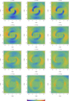 |
Fig. A.1. Same as Fig. 3, but for later times, t = 4.7 to 5.25 Gyr. |
| In the text | |
Current usage metrics show cumulative count of Article Views (full-text article views including HTML views, PDF and ePub downloads, according to the available data) and Abstracts Views on Vision4Press platform.
Data correspond to usage on the plateform after 2015. The current usage metrics is available 48-96 hours after online publication and is updated daily on week days.
Initial download of the metrics may take a while.