© The Authors 2025

1. Introduction

Relativistic outflows are common among astrophysical phenomena featuring accretion and/or explosions. Such outflows are observed as sources of bright non-thermal emission, indicating conversion of their kinetic energy into radiation. Internal shocks, collisions between parts of the outflow with different velocities, are one of the proposed dissipation mechanism in many astrophysical contexts. They were first introduced by Rees (1978) to explain “knots,” which are resolved inhomogeneities in the jet of galaxy M87 and were subsequently invoked to explain emission of radio-loud quasars (Spada et al. 2001), microquasars (Kaiser et al. 2000; Malzac 2014), and GRBs (Rees & Mészáros 1994; Sari & Piran 1997; Kobayashi et al. 1997; Daigne & Mochkovitch 1998). Internal shocks arise naturally when assuming inhomogeneities in the (proper) velocity of the outflow. In this scenario, a faster shell catches up with a slower one ejected at an earlier time by the central engine. The shells collide, and under the right conditions (see e.g., Pe’er 2014, for a review) two shock fronts will form: a forward shock (FS) propagating into the slow shell and a reverse shock (RS) propagating into the faster one. Particle acceleration is expected at these shock fronts, which consequently powers the emission from the outflow.

A common approach used to calculate the dissipation efficiency and calculate the emissions from internal shocks assumes plastic collisions: shells merge inelastically and continue propagating as a single shell (Daigne & Mochkovitch 1998; Beloborodov 2000; Spada et al. 2000; Guetta et al. 2001; Bošnjak et al. 2009; Malzac 2014; Bustamante et al. 2017; Rudolph et al. 2022, 2023). The energy dissipation is associated to a FS if the Lorentz factor (LF) of the fused shell is closer to the fast shell, or to a RS otherwise. While providing a useful approximation that allowed us to reproduce a number of features associated with internal shocks, this approach crudely approximates the location of the shock front. Seveveral studies have focused on the shock physics (e.g., Kino et al. 2004; Pe’er et al. 2017), but without considering the temporal evolution for a generic parameter space. This type of work was done by Rahaman et al. (2024a) (hereafter R24a), who provided an analytical framework for internal shocks between two cold, homogeneous, unmagnetized shells of arbitrary proper velocities in planar geometry.

This hydrodynamical framework is then completed with the parametrization from Genet & Granot (2009) for the optically thin synchrotron emission of a single shock front propagating over a range of radii. They found an analytical solution for the observed flux using integration over the equal arrival time surface (EATS) for a Band function spectral shape. Rahaman et al. (2024b) (hereafter, R24b) built their model on this basis, adding refinements such as the ratio between shock front LF and downstream fluid LF, while also considering the contribution from both shock fronts using the estimates obtained in R24a. This allowed them to self-consistently calculate the flux of a single collision at any observed frequency, which can then be used as a building block for full light curves and/or spectra of relativistic outflows. In this framework, the relative positions of the shock fronts and its dependency on the initial conditions are an important factor for the shape of the observed light curve, a feature that tends to get washed away by the ballistic approach. While the choice of initial conditions in most papers exploring the internal shock model for the GRB prompt emission have led to a very short-lived FS of negligible contribution to the total emission, the choice made in R24b led to the contributions from the two fronts covering similar timescales. This allowed the FS to convert enough energy to have a sizable contribution to the emission, producing a two-component time-resolved spectrum. This physical scenario for prompt GRB emission may provide an explanation for the significant deviations from the pure Band function fit (Band et al. 1993) in the time-resolved analysis of the brightest bins of observed bursts (Preece et al. 2014; Vianello et al. 2018).

The hydrodynamical solution is significantly simplified in the planar case, which is a decent approximation as long as the dissipation radius varies by a factor ≲2 during the shock propagation. In particular, the shock strengths remain fixed with time or radius in that case. Because of this R24a determined all quantities in planar geometry, and R24b introduced spherical effects on the peak frequencies and luminosities in an approximated manner by neglecting variation of the shock fronts LF and shock strength with time. Considering that such effects may modify the emission signature significantly, a fully consistent spherical approach is necessary to properly quantify the applicability of R24b results.

The present study focuses on the construction of the thin-shell synchrotron emission corresponding to the thin cooling layer behind the shock in the fast-cooling regime of spherical colliding shells through numerical simulations. In Sect. 2, we introduce the physical framework of this study, beginning with a summary of the main results from R24a (Sect. 2.1), followed by a presentation of the numerical code (Sect. 2.2), the model used to derive observed flux from our simulation results (Sect. 2.3), and finishing with the numerical setups for this study (Sect. 2.4). We present the results in Sect. 3, starting with the comparison of our fiducial spherical run with the planar case (Sect. 3.1) before exploring the fully spherical regime over the doubling radius (Sect. 3.2). Our calculated observed flux is presented in Sect. 3.3, then we present a study of the behavior of its peaks (Sect. 3.4) and try to derive information on the source activity from a few selected GRBs using those results (Sect. 3.5). Finally, we offer our first insights into the cooling effects on the observed spectra through an approximated marginally fast-cooling regime (Sect. 3.6). We present our conclusions and discuss our results in Sect. 4.

2. Physical scenario and numerical methods

2.1. Hydrodynamical framework

In R24a, the authors showed that the collision of two homogeneous cold relativistic shells is determined by seven basic parameters, which are presented Table 1: the time, t_off, between the ejection of the two shells, their proper speeds (u₁,u₄), where u≡Γβ, along with initial radial widths (Δ_0,1,Δ_0,4) and initial kinetic energies (E_k0,1,E_k0,4). Here and elsewhere, the subscript 0 denotes the initial values of properties, namely, at ejection or at the collision radius. Alternatively, the activity time (t_on,1,t_on,4) and the power (L₁,L₄) of the source during the emission of the shells may be used in place of the shells width and kinetic energy for a set of parameters focused on the source activity. The two are easily related through Δ_0,i=β_ict_on,i and E_k0,i=L_it_on,i, assuming constant jet power and outflow velocity within each ejection interval. In particular, the assumption of no velocity spread within a shell means that all fluid elements move at the same velocity and its width does not change during propagation. As shown in Table 2, those seven parameters can be combined into four derived parameters required to describe the post-collision shock hydrodynamics: the collision radius, R₀, the shells’ radial widths ratio, χ, the proper velocities ratio, a_u, and the proper density ratio, f. We also introduced the collision time t₀=R₀/β₄c in the source frame, where we implicitly chose t = 0 at the ejection of the front of shell 4. The shells were assumed to be cold, p₁=p₄ = 0, and the proper density of shell i was obtained from

$${\rho }_{\mathrm{i}}^{\prime }=\frac{1}{{\mathrm{\Gamma }}_{\mathrm{i}}({\mathrm{\Gamma }}_{\mathrm{i}}-1)}\frac{E_{\mathrm{k}0,\mathrm{i}}}{4\pi R_0^2{\mathrm{\Delta }}_{0,i}{c}^2},$$(1)

where primes denote quantities measured in the rest frames of the corresponding fluids. The collision of the two shells produces a pair of shocks: a reverse shock (RS) propagating into shell 4 and a forward shock (FS) propagating into shell 1. The two shocked regions, region 3 (shocked shell 4) and region 2 (shocked shell 1), are separated by a contact discontinuity (CD). At the collision radius, the use of the shock jump conditions together with pressure equality across the CD and the equation of state (EoS) in the shocked regions allow for an analytical derivation of all relevant hydrodynamical quantities. Values at the collision radius are noted with the subscript 0.

In planar geometry, quantities are constant across a shocked shell and with propagation. From the constant shock front velocities one easily derives shock crossing times and radii, determining the emission timing properties. In Appendix A, we present the main results from R24a. Those do not hold anymore in spherical geometry, prompting the present numerical study.

2.2. Numerical method

This study was performed with the code GAMMA (Ayache et al. 2022) with the aim to solve the equations of special relativistic hydrodynamics (SRHD) in one dimension, using a finite-volume Godunov scheme, the HLLC (Mignone & Bodo 2005) solver for relativistic hydrodynamics, piecewise linear spatial reconstruction, and following an arbitrary Lagrangian-Eulerian approach. This means GAMMA can compute fluxes for any interface velocity. The HLLC solver adds a calculation of the contact discontinuity (CD) wave speed to the two-wave HLL solver (Harten et al. 1983), the default behavior of GAMMA sets the interface velocity to that of the CD. We used this default setting throughout the entirety of this work, as a mesh moving with the flow's velocity evolves propagating shells over a wide range of scales using bigger time steps: in such a mesh, the limiting velocity becomes the sound speed; whereas in fixed-mesh approaches, it would be the flow speed instead. Such a moving mesh also offers the added benefit of Lagrangian behavior of the cells like natural refinement of zones with high gradients, as the cell size will follow the compression of the fluid.

GAMMA offers the choice between several time integration methods, among which we chose the third-order Runge-Kunta. The time step is adaptive, based on a Courant-Friedrich-Lewy (CFL) condition (Courant et al. 1928). To be consistent with the derivation of R24a, we implemented the Taub-Mathews equation of state (Mathews 1971) following Mignone & McKinney (2007). We used none of the adaptive mesh refinement methods present in GAMMA because we wanted to be able to properly identify cells from one time step to the next and compare their properties. Finally, we use the shock detection algorithm introduced in Zanotti et al. (2010) already implemented in GAMMA. We found setting the shock detecting threshold to 0.15 produces satisfactory detections of the two fronts across the simulation. GAMMA also contains a method to inject an electron distribution in shocked cells and let them evolve using a reformulation of the cooling equation into an advection equation, which we did not use in this work given our choice of assumptions for the radiative efficiency (see discussion in Rahaman et al. 2024b, and references therein). We leave the exploration of different cooling regimes to a future work.

2.3. Flux calculation from cells

In this study, we derived the observed flux from our simulations by applying the method for an infinitely thin shell, as described in Genet & Granot (2009), to cells right downstream of each shock front. Here, the infinitely thin shell approximation is validated as Δr/R∼10⁻⁹ for shocked cells in the simulations run for this work. The contributing cells are chosen right downstream of the shocks, counting only one contribution of each cell crossed by the shock, waiting the few time steps necessary for the shock to cross to another cell to add a new contribution. We also assumed the accelerated electrons follow a power-law energy distribution of index p (${\mathit{dN}}_{\mathrm{e}}/d{\gamma }_{\mathrm{e}}\propto {\gamma }_e^{-p}$ for γ_e≥γ_m) and all the energy given to the electrons of a cell by the shock passage is radiated in less than a numerical time step. This requires the emission to be deep in the “fast-cooling” regime. After identifying the contributing cell right downstream of the shock, we derived the minimum Lorentz factor of the post-shock electron distribution by normalizing the total available energy over the electron population:

$${\gamma }_{\mathrm{m}}=\frac{p-2}{p-1}\frac{m_{\mathrm{p}}}{m_{\mathrm{e}}}\frac{{ϵ}_{\mathrm{e}}}{{\xi }_{\mathrm{e}}}\frac{e_{\mathrm{int}}^{\prime }}{{\rho }^{\prime }{c}^2}\hspace{0.5em},$$(2)

for p>2, where $e_{\mathrm{int}}^{\prime }$ is the comoving (or proper) internal energy density; ϵ_e is the fraction of internal energy transferred to the fraction ξ_e of total electrons. For this study, we assumed an equipartition of energy ϵ_e=ϵ_B = 1/3 and chose values of p = 2.5, ξ_e = 10⁻² for the accelerated electron distribution power-law index and fraction of accelerated electrons respectively. To this Lorentz factor corresponds the comoving peak frequency

$${\nu }_{\mathrm{m}}^{\prime }={\nu }_{\mathrm{syn}}^{\prime }({\gamma }_{\mathrm{m}})=\frac{q_{\mathrm{e}}{B}^{\prime }}{2\pi m_{\mathrm{e}}c}{\gamma }_{\mathrm{m}}^2.$$(3)

The contribution of a cell at radius r and time t traveling with dimensionless velocity β (corresponding to the Lorentz factor Γ) to the flux at an observed frequency, ν, and observed time, T, is:

$$F_{\nu }(\tau \ge 1)=\frac{1+z}{4\pi d_{\mathrm{L}}^2}{\tilde{L}}_{{\nu }_{\mathrm{m}}}{\tau }^{-2}S\left(\tau \frac{\nu }{{\nu }_{\mathrm{m}}}\right),$$(4)

where S is a normalized function verifying S(x) = xS(x) = 1 for x = 1. The normalized time, τ, is defined as

$$\tau =\frac{T-T_{\mathrm{ej}}}{T_{\theta }},T_{\mathrm{ej}}=(1+z)\left(t-\frac{r}{\beta c}\right),T_{\theta }=\frac{(1+z)r}{2{\mathrm{\Gamma }}^{2}c},$$(5)

and the peak luminosity is

$${\tilde{L}}_{{\nu }_{\mathrm{m}}}=\frac{\mathrm{\Gamma }\mathrm{\Delta }{V}^{(3)}}{T_{\theta }}\frac{{ϵ}_{\mathrm{e}}{e}_{\mathrm{int}}^{\prime }}{W(p){\nu }_{\mathrm{m}}^{\prime }}.$$(6)

Here, ΔV⁽³⁾ is the (three-)volume of the cell in the rest frame of the central source and W(p) = 2(p−1)/(p−2). We obtained Eq. (6) by comparing the isotropic energy from a single pulse in the formulation of GG09 and the formulation of De Colle et al. (2012). The derivation is detailed in Appendix B.2. The quantity ${\tilde{L}}_{{\nu }_{\mathrm{m}}}$ is a numerical equivalent luminosity derived from synchrotron power and is not to be confused with the usual luminosity that appears in similar equations for the flux in GG09 or R24b. From their Appendix D, we can express the comoving luminosity behind a shock front:¹

$$L_{{\nu }_{\mathrm{m}}^{\prime }}^{\prime }=\frac{L_{\mathrm{bol}}^{\prime }}{W(p){\nu }_{\mathrm{m}}^{\prime }}=\frac{4}{3}\pi R^2{\beta }_{\mathrm{ud}}c\frac{{ϵ}_{\mathrm{e}}{e}_{\mathrm{int}}^{\prime }}{W(p){\nu }_{\mathrm{m}}^{\prime }}\hspace{0.5em},$$(7)

using $e_{\mathrm{int}}^{\prime }=({\mathrm{\Gamma }}_{\mathrm{ud}}-1){\rho }_{\mathrm{d}}{c}^2$ to obtain β_ud. Finally we identified:

$${\tilde{L}}_{{\nu }_{\mathrm{m}}}=\frac{3\mathrm{\Gamma }\mathrm{\Delta }r}{{\beta }_{\mathrm{ud}}{\mathit{cT}}_{\theta }}{L}_{{\nu }_{\mathrm{m}}^{\prime }}^{\prime }.$$(8)

In this work, the spectral shape, S, will either be the synchrotron broken power law with low- and high-frequency spectral slopes, b₁ and b₂, respectively (syn-BPL), or the Band function:

$$S(x)=e^{1+b1}\{\begin{array}{cc}{x}^{b_1}{e}^{-(1+b_1)x}\hfill & x\le x_{\mathrm{b}},\hfill \\ x^{b_2}{x}_{\mathrm{b}}^{b_1-b_2}{e}^{-(b1-b2)}\hfill & x\ge x_{\mathrm{b}},\hfill \end{array}$$(9)

where x_b=(b₁−b₂)/(1+b₁). Following R24b, the choice of setting both fronts deep in the fast-cooling regimes sets values of b₁=−1/2 and b₂=−p/2=−1.25 for spectral slopes. This choice is further discussed in the conclusion. The effect of setting the weaker FS in the marginally fast-cooling regime is discussed in Sect. 3.6. Summing all contributions from the run gives the total observed flux as a function of observed time and frequency.

In the following, quantities are plotted in units of the normalization frequency, ν₀, and flux, F₀, defined as the peak observed frequency and flux radiated at the RS at collision in R24b:

$${\nu }_0=2{\mathrm{\Gamma }}_0{\nu }_{\mathrm{m},\mathrm{RS}}^{\prime }(R_0),$$(10)

$$F_0=\frac{(1+z)}{12\pi d_{\mathrm{L}}^2}2{\mathrm{\Gamma }}_0{L}_{{\nu }_{\mathrm{m}}^{\prime },\mathrm{RS}}^{\prime }(R_0).$$(11)

Here, Γ₀ is the Lorentz factor of the shocked material at R₀, which is at this radius equal downstream of both shock fronts. We refer to their Appendix G for the full derivation. Here, we write $\tilde{\nu }=\nu /{\nu }_0$ as the normalized frequency and $\tilde{T}=1+\overline{T}=(T-T_{\mathrm{ej},0})/T_{\theta ,0}$ as the normalized time – as defined in Eq. (5) with the relevant values at t₀ and R₀.

2.4. Numerical setup

To expand on the theoretical framework of R24b, we explored the collision of two ultrarelativistic shells of equal energy and width with a moderate proper velocity ratio of a_u = 2. The kinetic energy available in the shells is taken to be 10⁵² erg, a typical order of magnitude value for the isotropic equivalent value corresponding to a single GRB pulse. The choice of equal activity time and equal shell width is doubly motivated by the GRB spectrum observations and to ensure a high radiative efficiency. From R24b, the peaks’ relative prominence is tied to the shells’ sizes: if t_on,1≳2 t_on4, the FS peak is too prominent relative to the RS and vice versa (see e.g., their Fig. 4). They also showed that the rarefaction wave traveling back towards the center after shock crossing may catch up with and suppress the second shock before it finishes crossing its shell. This is valid for values of χ that are not close to 1, limiting the radiative efficiency of the process in such a case. The off time between pulses, t_off, is set to the same value as the pulses themselves, as observations suggests a correlation between pulse width and interval between pulses, outside of quiescent periods (see e.g., Nakar & Piran 2002). We set both activity times, t_on, and the off time to a typical order of magnitude for the activity timescale of 0.1 s. The shells are ultrarelativistic with Lorentz factors of u₁ = 100 and u₄ = 200, which are minimum values to ensure the assumption of optically thin emission.

To complete this setup, we defined the external medium density behind shell 4, ${\rho }_{\mathrm{ext},\mathrm{b}}^{\prime }$ and in front of shell 1, ${\rho }_{\mathrm{ext},\mathrm{f}}^{\prime }$ from a density contrast parameter of ${\tilde{\rho }}_{\mathrm{ext}}^{\prime }={\rho }_4^{\prime }/{\rho }_{\mathrm{ext},\mathrm{b}}^{\prime }={\rho }_1^{\prime }/{\rho }_{\mathrm{ext},\mathrm{f}}^{\prime }$. Both regions of the external medium were set with the same velocity as the shell they are in contact with. Such an “external” medium is required for the rarefaction wave to set after shock crossing and hardly affects the results. The external pressure is defined by introducing the relativistic temperature, Θ₀, as a parameter, we set the pressure to be constant everywhere, namely, as $p_0=min({\rho }_1^{\prime },{\rho }_4^{\prime }){\mathrm{\Theta }}_0{c}^2$. Setting the pressure equally over the whole simulation box avoids any unwanted effects from pdV working between the external medium and the shells. All these parameters are summarized in Table 3. The simulation was run in 1D over 6100 cells, of which there are N_sh = 3000 for each shell and 50 on each side for the external medium. This choice of the resolution was meant to ensure that the shock fronts have not propagated more than 2×10⁻³R₀ before the downstream values are properly established. This can be estimated by applying the formula for the crossing time (Eq. (A.3)) to the width of five numerical cells, greater than the typical numerical size of the detected shock front with our choice of threshold parameter. Finally, we set an additional passive tracer with different values in each shell to help separate them easily during post-processing.

To fully explore the effects of spherical geometry on shock hydrodynamics by going well above the doubling radius for the crossing radius of each front, we ran another simulation in spherical geometry with larger activity times (and initial shells width) by a factor of 5. Meanwhile, we kept the off time constant. We increased the number of numerical cells per shell by the same factor. The values corresponding to this run are given in brackets in Table 3.

3. Effects of spherical geometry

Having calibrated our simulation against the analytical results in planar geometry in Appendix A, we explored the spherical effects through two simulations. In the first, all parameters are equal for the sake of comparison and in the second, the activity times t_on,i (and, thus, the shell width Δ_0,i) have been multiplied by 5 to explore hydrodynamics over a larger range of radii.

3.1. Spherical effects on shells structure and shock dynamics

A first result of performing the same run in spherical geometry is the variation in crossing times (radii): for the same values of parameters, ΔR_RS/R₀ increases from 1.29 to 1.52 when switching from planar to spherical geometry, while ΔR_FS/R₀ only grows from 1.62 to 1.67. Figure 1 displays snapshots of the comoving density, proper velocity, and pressure (similarly to Fig. A.1) at times t₀, 2 t₀, and 2.6 t₀. In the analytical expectations from planar geometry, the density and pressure are rescaled by (R/R₀)⁻² to account for propagation, then plotted to better highlight the differences with R24a. Spherical effects modify the structure of the shocked regions: the density profile shows compression from the shocks to the contact discontinuity, a proper velocity decrease with radius, and a slightly increasing pressure profile from the RS to the FS. As the shells and shocks propagate, the density in regions 1 and 4 (i.e., the unshocked portions of both shells) will decrease with r⁻². This is due to mass conservation of a fluid element in spherical geometry, with our assumption of little to no velocity spread between the two interfaces. At the zeroth order, where we consider constant shock strength, the downstream density, ρ_d, and pressure will also evolve following a r⁻² law. From pressure continuity (i.e., the pressure gradient is rather small in the shocked regions as they are in causal contact), the pressure at the CD will follow the same law instead of the $r^{-2\hat{\gamma }}$ from adiabatic expansion, with $\hat{\gamma }$ being the adiabatic index. Specifically, $p_d\approx p_0(R/R_0{)}^{-2}\approx p_{\mathrm{CD}}\approx ({\rho }_{\mathrm{CD}}/{\rho }_0{)}^{\hat{\gamma }}$ and ρ_d=ρ₀(R/R₀)⁻², implying ${\rho }_{\mathrm{CD}}/{\rho }_d=(R/R_0{)}^{2(1-{\hat{\gamma }}^{-1})}$. This results in a compression of the fluid towards the center with the ratio between densities behind the shock and at the CD following a $-2(1-{\hat{\gamma }}^{-1})$ law. This implies a density scaling ${\rho }_{\mathrm{CD}}\propto r^{-2/\hat{\gamma }}$ between r^−1.5 and r^−1.2 (${\rho }_{\mathrm{CD}}/{\rho }_{\mathrm{d}}\propto r^{2(1-{\hat{\gamma }}^{-1})}$ between r^0.5 and r^0.8) for an adiabatic index varying between 4/3 and 5/3.

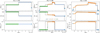Fig. 1. Snapshots of the run in spherical geometry, with all parameters similar to the fiducial run, at t=t0 (left), before first (reverse) shock crossing (center), and after shock crossing (right). Dashed black lines show the analytical expectations from the results in planar geometry. The legend is the same for all panels.

Both of these effects are seen Fig. 2 (top panel) which displays densities rescaled with (r/R₀)² to take out spherical effects: the values taken right downstream of the shocks show very little to no variation in radius, while those on both sides of the CD increase with the same r^0.7 (or ρ′∝r^−1.3 without rescaling) fitting with our observed regime of intermediate shock strengths. This results in intermediate adiabatic index values according to the Kumar & Granot (2003) formulation used in R24a:

$$\hat{\gamma }=\frac{4{\mathrm{\Gamma }}_{\mathrm{ud}}+1}{3{\mathrm{\Gamma }}_{\mathrm{ud}}},$$(12)

which those authors demonstrated is equivalent to the Taub-Mathews EoS for a cold upstream medium. To a highest order of precision, the variation of the shock strength Γ_ud−1 with propagation changes this behavior; as seen in the bottom panel of Fig. 2, the shock strengths decrease with propagation at a stronger rate for the RS than the FS. This translates to a slight decrease in the post-RS rescaled density and stronger decrease in the post-RS pressure than that seen downstream of the FS (as shown in the 3rd panel of Fig. 2). This explains the increasing pressure profile from RS to FS seen in the snapshots. Similarly, we observed a higher post-RS flow velocity than that seen downstream of the FS, where the first increases with propagation, while the second decreases with it, creating the profile observed Fig. 1. In terms of power-law scalings, this approach has proven useful to explain behavior below the doubling radius (i.e., R≲2R₀); however, when exploring a broader range of radii, a different behavior is observed above it.

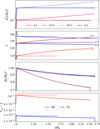Fig. 2. Top to bottom: comoving densities, Lorentz factors of the fluid and shock fronts, pressure, and shock strengths. The hydrodynamical quantities are measured downstream of shocks (‘d,3’ downstream of the RS, ‘d,2’ for the FS), at the CD by averaging over a few cells crossing the interface, or on each side of it (CD3, CD2) for the density. Legend is the same for all panels. The derived Lorentz factor of the shock fronts is displayed with the measured ones. Densities and pressures are in units of the values behind the RS in the planar case and rescaled to (r/R0)2. We smoothed the numerical oscillations in data by a rolling average. Horizontal dashed lines show the corresponding analytical values from R24a.

3.2. Asymptotical hydrodynamics in the spherical regime

We present the results of the simulation run with both activity times multiplied by a factor of 5, while keeping t_off and all other quantities constant. This means the shells are now wider than their separation by this same factor, allowing us to explore the evolution of the various relevant quantities for the flux calculation over a range of radii ∼10 R₀, almost an order of magnitude greater than the situation presented in Sect. 3.1. In Fig. 3, we show the fluid and shock fronts Lorentz factors in the top panel and the shock strengths in the bottom panel. The data were smoothed by a rolling average window to eliminate the strong noise caused by the propagation of numerical errors in the interface velocity over the large number of code iterations for this simulation. Such oscillations could be reduced by the use of an higher spatial order reconstruction algorithm instead of the first-order piecewise linear algorithm currently present in GAMMA. The downstream and shock Lorentz factors evolve at the same rate, keeping the ratio g=Γ/Γ_sh introduced in R24a close to constant. At the collision radius, the values are in accordance to the analytical expectations in planar geometry derived in R24a, before decreasing in a power-law up to the doubling radius and smoothly connecting to a constant value after a few R₀. Values relative to the RS change by a greater amount in this asymptotical regime compared to the planar case than values relating to the FS: the shock and downstream Lorentz factor grow by ∼10 % at the RS and go down by ∼3% at the FS, while the shock strength diminishes by ∼3% and ∼0.7%, respectively. Thus, we modeled any hydrodynamical or derived quantity X with the law:

$$X(R)={\left[{\left(X_{0*}{\tilde{R}}^n\right)}^s+{\left(X_{\mathrm{sph}}{\tilde{R}}^h\right)}^s\right]}^{1/s}=X_0{f}_X(R),$$(13)

with $\tilde{R}=R/R_0$ and f_X a function verifying f_X(R₀) = 1. The index h corresponds to the expected scaling from propagation effects at constant shock strength, which can be 0. Then, $X_{\mathrm{sph}}{\tilde{R}}^h$ is the asymptotical value at large radii and X_0* is defined by the value at collision radius $X_0=X(R_0)=[X_{0*}^s+X_{\mathrm{sph}}^s{]}^{1/s}$. We note that s values need to be of the opposite sign of n (and of h when nonzero). The values obtained for the shock strength and downstream Lorentz factors by the fitting procedure are given Table 4. While the change in those quantities and thus the related quantities such as luminosity and peak frequency are not very significant in absolute values, it is their rate of change that has the most impact on the observable data at very early times.

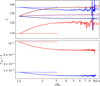Fig. 3. Top: Lorentz factors of the shock fronts, the fluid downstream of the shocks and at the CD with radius. Bottom: evolution of shock strengths with radius. Data were smoothed by rolling average. The quantities converge smoothly to a constant value after r≈4R0, shown by the dotted horizontal line for the quantities relative to the RS and the FS. Legend is the same as in Fig. 2.

3.3. Emission from two spherical colliding shells

In Figs. 4 and 5, we present the resulting light curves and time-integrated spectra from our simulations, comparing the two geometries in the same panel for both the Band and the broken power-law spectral shapes. To highlight the difference between the assumptions for propagation chosen in R24b and the fully spherical results, we compare our results to the hybrid approach instead of the fully planar case detailed in Appendix B.3. The total light curve is weakly affected by the geometry, with slightly increased peak times corresponding to our estimation in Sect. 3.1 and a smoothed shape compared to the planar case. In comparison, the individual contributions of each shock front vary significantly, with the RS peak luminosity increasing by a factor of 1.25 and that of the FS decreasing by a factor of 0.7.

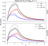Fig. 4. Light curves in the spherical (full lines) and hybrid (planar geometry and spherical assumptions for peak frequency and luminosity, dash-dotted lines) cases at fixed frequency $\tilde{\nu }=0.1$. Top panel: light curves with the Band's spectral shape. Bottom panel: broken power-law spectral shape. The total light curve in the hybrid + Band case is redrawn in the bottom panel (dotted line) for the sake of comparison. The individual contributions from each shock change but the resulting light curve do not, apart from the slightly increased breaks from the increase in crossing times. The choice of spectral shape decreases total emission at this frequency, while keeping the same time evolution.

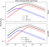Fig. 5. Time-integrated spectra following the same structure as in Fig. 4. The spherical effects decrease the peak frequencies for both shocks, with a stronger effect on the RS. The peaks from both contributions are closer than in the planar case, resulting in a three-part spectrum. This effect is more visible with the broken power-law spectral shape where the two peaks are distinct from each other in the hybrid approach. The choice for the spectral shape also diminishes the flux at low frequencies.

The time-integrated spectra in Fig. 5 show the peak frequencies of both shock fronts decrease by different amounts: the quantities relative to the RS decrease faster with radius than those relative to the FS. Thus, the observed range of the frequencies ratio between the two spectral components can be attained with a wider range of a_u in this fully spherical approach. From the hybrid approach, we retained the doubly broken power-law spectrum with indices 1+b₁ = 0.5 and 1+b₂=−0.25 at low and high energies, directly related to our choice of synchrotron spectral slopes, and an intermediate part 1+b_mid≈0.1. The effective middle slope b_mid depends on the flux normalization for each front and is thus very variable with the choice of hydrodynamical conditions: an analytical estimate using R24b show 1+b_mid∈[−0.05,0.45] when exploring the parameter space (χ,a_u)∈[−0.5,1.5]×[1.01,5], under the assumptions of ultrarelativistic shells and constant central engine power. These slopes are the same for both the Band and syn-BPL spectral shapes. The differences between the results of this present study and those from R24b are highlighted by redrawing in dotted line the Band + hybrid light curve (respectively, the time-integrated spectrum) in the syn-BPL panel. The main change lies in the total received flux (respectively, the fluence), especially at lower frequencies, but the essential characteristics of the light curve (respectively, the time-integrated spectrum) are similar.

3.4. Peak frequency and flux

The individual variations of peak frequency and flux associated to each shock front are displayed in Fig. 6 against normalized time, where the spherical effects systematically lowers both the peak frequency and flux for both shocks. The spherical geometry also introduces a difference in the time evolution of the peak frequency between the rising and the high-latitude emission (HLE) part. While the flux rises, the peak frequency decreases faster than ${\nu }_{\mathrm{pk}}\propto {\tilde{T}}^{-1}$ expected from purely geometric considerations. This is especially the case for the RS, with ${\nu }_{\mathrm{pk},\mathrm{RS}}\propto {\tilde{T}}^{-1.9}$. In the following, we present a way to estimate those quantities from the hydrodynamics with fewer calculations than the full flux calculation (detailed in Sect. 2.3). We built this approach on the asymptotical regimes identified for the hydrodynamical quantities in Sect. 3.2.

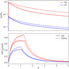Fig. 6. Normalized time evolution of peak frequency and flux for both shock fronts in the spherical (full line) and hybrid (dash-dotted) cases, calculated from the flux obtained with the Band spectral shape. In spherical geometry, the peak frequency decrease at a faster rate during the rising phase and the flux reaches saturation before the break to the high-latitude emission.

Assuming the hydrodynamical variables can be modeled according to the law given by Eq. (13), after extracting the relevant variables for flux calculation from the simulation results, we fit them with the same type of law:

$${\mathrm{\Gamma }}_{\mathrm{d}}(R)={\left[{\left({\mathrm{\Gamma }}_{0*}{\tilde{R}}^{-m/2}\right)}^s+({\mathrm{\Gamma }}_{\mathrm{sph}}{)}^s\right]}^{1/s}\equiv {\mathrm{\Gamma }}_{\mathrm{f},0}{f}_{\mathrm{\Gamma }}(R)\hspace{0.5em},$$(14)

$${\nu }_{\mathrm{m}}^{\prime }(R)={\left[{\left({\nu }_{0*}^{\prime }{\tilde{R}}^d\right)}^s+({\nu }_{\mathrm{sph}}^{\prime }{\tilde{R}}^{-1}{)}^s\right]}^{1/s}\equiv {\nu }_{\mathrm{f},0}^{\prime }{f}_{{\nu }^{\prime }}(R)\hspace{0.5em},$$(15)

$$L_{{\nu }_{\mathrm{m}}^{\prime }}^{\prime }(R)={\left[{\left(L_{0*}^{\prime }{\tilde{R}}^a\right)}^s+(L_{\mathrm{sph}}^{\prime }\tilde{R}{)}^s\right]}^{1/s}\equiv L_{\mathrm{f},0}^{\prime }{f}_{L^{\prime }}(R)\hspace{0.5em}.$$(16)

We performed the fit with the curve_fit function from SciPy, which is based on a non-linear least square method. We give in Table 4 the obtained values for the fits. The numerical values at R₀ differ slightly (≲2%) from the analytical expectations, we note them with the subscript “f,0” to avoid confusion.

Then, to obtain an estimate for the peak frequency and flux in the rising part of the prompt emission, we assume we can define an effective radius on the EATS at which the peak contribution can be calculated R_eff(T) = y_effR_L(T), with R_L(T) as the maximal radius of the EATS (found along the line of sight). At a given observer time, T, this radius can also be identified by its angle with the line of sight – or, more conveniently, by the quantity ${\xi }_{\mathrm{eff}}=(\mathrm{\Gamma }\theta {)}_{\mathrm{eff}}^2$. A schematic of this method is given Fig. C.1.

Both quantities are joined by $\mathit{y}={\left[1+g^{-2}\xi \right]}^{-1}$ and we take $R_{\mathrm{L}}=R_0\tilde{T}$, where we implicitly choose a constant Γ_sh to approximate the EATS at the zeroth order. Then, the peak frequency and flux are given by:

$$(1+z){\nu }_{\mathrm{pk}}(T)=k_{\nu }{\nu }_{\mathrm{f},0}\frac{f_{\mathrm{\Gamma }}(R_{\mathrm{eff}})f_{{\nu }^{\prime }}(R_{\mathrm{eff}})}{1+{\xi }_{\mathrm{eff}}},$$(17)

$$F_{{\nu }_{\mathrm{pk}}}(T)=k_F{F}_{\mathrm{f},0}3g^2{\xi }_{\max }{\left(\frac{f_{\mathrm{\Gamma }}(R_{\mathrm{eff}})}{1+{\xi }_{\mathrm{eff}}}\right)}^3\frac{f_{L^{\prime }}(R_{\mathrm{eff}})}{f_{\mathrm{\Gamma }}(R_{\mathrm{L}}{)}^2}.$$(18)

Here, ${\nu }_{\mathrm{f},0}=2{\mathrm{\Gamma }}_{\mathrm{f},0}{\nu }_{\mathrm{f},0}^{\prime }$ and $F_{\mathrm{f},0}=\left((1+z)/(4\pi d_{\mathrm{L}}^2)\right)2{\mathrm{\Gamma }}_{\mathrm{f},0}{L}_{\mathrm{f},0}^{\prime }$. k_ν and k_F are two free parameters of order unity introduced to compensate for the difference between analytical and numerical values at R₀ such that k_νν_f,0=ν₀ and k_FF_f,0=F₀. The observed peak frequency is obtained by calculating the Doppler factor and comoving peak frequency at R_eff, and the flux is obtained by assuming the flux integral (Eq. (B.7)) can be approximated by the value of the integrand at ξ_eff times the extension of the EATS in this variable, ${\xi }_{\max }=g^2(\tilde{T}-1)$. We then looked for the function ξ_eff(T) fitting the data. We note that contributions from regions of the EATS beyond the relativistic beaming angle 1/Γ become increasingly suppressed, thus, we defined a saturation angle ξ_sat on the order of unity and we chose the following fitting function for ξ_eff:

$${\xi }_{\mathrm{eff}}(T)=k_{\xi }{\left({\xi }_{\max }^{-s}+{\xi }_{\mathrm{sat}}^{-s}\right)}^{-1/s}=k_{\xi }{\left({\left[g^2(\tilde{T}-1)\right]}^{-s}+{\xi }_{\mathrm{sat}}^{-s}\right)}^{-1/s},$$(19)

where k_ξ, ξ_sat, and s are free parameters. The high-latitude emission part is modeled as the emission from the final effective radius R_eff,f=y_eff(T_f)R_f, with T_f the observed time corresponding to the shock crossing:

$${\nu }_{\mathrm{pk},\mathrm{HLE}}(T)={\nu }_{\mathrm{pk}}(T_{\mathrm{f}}){\tau }_{\mathrm{f}}^{d_{\nu }}\hspace{0.5em},$$(20)

$$F_{{\nu }_{\mathrm{pk},\mathrm{HLE}}}(T)=F_{{\nu }_{\mathrm{pk}}}(T_{\mathrm{f}}){\tau }_{\mathrm{f}}^{d_{\mathrm{F}}}\hspace{0.5em},$$(21)

and τ_f is the normalized time defined at R_eff,f following Eq. (5). We give in Table 5 the values found to fit the peak frequency and flux (from Fig. 6) with an accuracy within a few percent.

3.5. Maximal frequency and crossing radius

Among the spectral signatures, the behavior of the peak flux versus peak frequency shown in the left panel of Fig. 7 presents the most striking change between planar and spherical dynamics. In this figure, we compare the purely spherical case to the hybrid approach of R24b, which features planar dynamics along with spherical geometry for calculating the radiation. The spherical case transitions to the anticipated correlation of high-latitude emission $(\nu F_{\nu }{)}_{\mathrm{pk}}\propto {\nu }_{\mathrm{pk}}^3$ at a lower frequency but presents a high flux over a wider range. We define ν_bk as the peak frequency at this break. Comparing to Fig. I1 in R24a, the combined effects from spherical geometry on the peak flux and frequency is greater than a pure increase of ΔR/R₀ in the hybrid approach; simply increasing the crossing radius in the R24 formalism is not enough to obtain the curves in the spherical case.

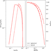Fig. 7. Left: νFν at peak frequency vs peak frequency for the reverse shock in the spherical and hybrid case. The fully spherical case show peak flux over a larger range of frequencies. Right: ratio between break frequency νbk and frequency at half flux ν1/2. Legend is the same for both panels.

In the right panel of Fig. 7, we display the evolution with a normalized crossed radius, ΔR/R₀. of the ratio between ν_bk and the frequency ν_1/2, defined as the point where the peak flux in the rising part is half that at ν_bk. This allows us to add our modifications to the results presented in Table I1 from R24b: from the ratio in frequencies for peak flux obtained from the data presented in Yan et al. (2024) and assuming the RS is the main contribution to the observed flux, they inferred the radius crossed by the RS during the burst ΔR/R₀ and, thus, the ratio of activity time to off time t_on,4/t_off. We present in Table 6 our updated values for the crossed radius in light of spherical effects and compare them to the values inferred in R24b. On average, the obtained crossed radius for our fiducial spherical case is half of the value obtained by R24b and about a third for the obtained activity over the off time ratio.

3.6. Dissipation efficiency and marginally fast-cooling regime

The total efficiency, ϵ_tot=ϵ_intϵ_eϵ_rad, of the internal shock process is easily derived in this framework. When it is deep in the fast-cooling regime, it implies a radiative efficiency of ϵ_rad = 1 behind both shock fronts. Here, ϵ_int is the conversion rate of kinetic energy into internal energy, commonly called the dissipation efficiency (or “thermal efficiency,” noted ϵ_th, in R24a,b). We calculate it by summing the internal energy from each contributing cell and comparing this quantity to the initial available kinetic energy. We obtained a dissipation efficiency of 8.5% in the planar case (equal to the analytical value using Eq. (B5) in R24b) and of 7.3% in the spherical case. The total efficiency is thus ϵ_tot = 2.4% in the spherical case. In R24a,b, the dissipation efficiency is obtained by comparing the total final internal energy present in the shells after shock crossing to the initial available kinetic energy. Both our “local” and their “global” approaches give the same result in the planar case, but the quantities are different in the spherical case due to the shock strengths evolving as they cross their respective shells. Using the definition R24a,b would give a dissipation efficiency of 3.5% in the spherical case.

The spectrum we obtained using this thin-shell assumption displays a low-energy νF_ν slope of 1+b₁ = 0.5, indicative from fast-cooling, which does not seem to fit observed bursts. In Ravasio et al. (2019), for instance, their fits using a doubly broken power-law model give values of the low-energy slopes from several bursts that are more consistent with a slow-cooling regime. While a model where cooling is derived consistently is beyond the scope of the current paper, we began to look into this issue by recalculating the contributions from the FS in an approximated marginally fast-cooling regime. For this, we took b_1,FS = 1/3 instead of −1/2 and we applied an efficiency factor of ϵ_rad,FS = 1/2 to the computed FS flux as in R24b. This value of 1/2 is an arbitrary middle ground between ϵ_rad,FC∼1 in the fast-cooling case and ϵ_rad,SC≪1 in the slow-cooling case. With this choice, we obtained an overall efficiency of the prompt emission ϵ_tot = 2% for the spherical simulation. We compare in Fig. 8 the instantaneous spectra at T=T₀ ($\overline{T}=1$) obtained in this marginally fast-cooling FS case with the fast-cooling regime. Both were calculated from the simulation in spherical geometry. For this marginally fast-cooling FS, we did not obtain the slow-cooling low-energy slope of 1+b_1,FS = 4/3, but rather ∼0.8 from the cumulative contribution of the two shock fronts.

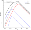Fig. 8. Comparison of instantaneous spectra between two fast-cooling shock fronts (full lines) versus a fast-cooling RS and a marginally fast-cooling FS (dash-dotted lines) at $\overline{T}=1$. The low energy slopes are steeper and the overall flux is lower with a marginally fast-cooling FS.

Setting the FS in the marginally fast-cooling regime is not enough to obtain low energy slopes more in line with observations from our set of simulations. However, we need to mention that marginally fast-cooling regime has three issues here. First, it requires a very specific set of physical conditions that is contrary to our general approach. Second, if the FS is marginally fast-cooling, the RS is not very deep in the fast-cooling regime, and should show a cooling break near the FS peak photon energy, below which 1+b₁ = 4/3 is expected in the total spectrum. Third, we used an approximated way of calculating the radiation in this regime, we expected the thin shell assumption to break and, thus, the effects of a finite size emission region to appear, which are bound to modify emission signatures. Such effects will be the focus of a follow-up paper dedicated to the exploration of the cooling regimes.

4. Conclusions

We present a fully spherical, self-consistent numerical approach to the internal shocks model for the prompt GRB emission, showing the impact of the spherical hydrodynamics effects on emission, even for crossing radii lower than twice the initial collision radius. Our basic two-shell collision model describes a single spike in the prompt GRB light curve, which usually consists of multiple pulses that in this picture correspond to multiple collisions. After calibrating our methods against the analytical results obtained in Rahaman et al. (2024a, b) using a planar approach for hydrodynamics and approximate spherical effects for the emission, we numerically extend their conclusions to the fully spherical case, while keeping the assumption of an infinitely thin emitting shell. We present the structural and dynamical differences of shocked shells in spherical geometry and highlight the non-negligible effects of the evolution in Lorentz factors and shock strengths on the emission over the shock crossing time. In particular, the quantities associated with each shock front evolve at a different rate due to the differences in shock strengths. We then expect that following the spectral properties of a burst over time will allow us to distinguish this two-zones emission model from a one-zone model. While we assumed equal values of the microphysical parameters (ϵ_e,ϵ_B,ξ_e,p) between the two shock fronts, any diversity in those parameters will most likely add diversity to the obtained emission between the two shock fronts.

We produced light curves and (time-integrated) spectra with two different spectral shapes, the smooth Band function and the synchrotron broken power law. While the Band function is a phenomenological model of the emission spectrum, the synchrotron broken power law is physically motivated. Calculating flux with the latter results in less flux at lower frequencies, but conserves the general time evolution of the light curve. In both choices of spectral shape, our framework naturally obtains a doubly broken power-law shape for the spectrum, shape that has been successfully used to fit prompt GRB data (see e.g., Burgess et al. 2014; Oganesyan et al. 2017; Ravasio et al. 2019). The validity of the results obtained with the rough spectral shape compared to using the empiric smooth Band function motivates the use of this simpler emission function to explore more complicated flows as well as other cooling regimes with different spectral shapes in further works while retaining physical accuracy. The value of the spectral slope between the two breaks varies significantly with the choice of initial conditions. While it is not totally consistent with the range of values obtained in Ravasio et al. (2019), this is not a contradictory result. Those slopes are more dependent on the choices made for the fitting functions than the low- and high-energy part and a better test of our model would be to perform fits of observed data from calculated flux across an expected parameter space.

While the effects of spherical geometry on the shock hydrodynamics are not striking when comparing light curves and time-integrated spectra, they cannot be ignored when studying the evolution of spectral shape within a single spike in the prompt GRB light curve. In particular we obtain shapes that are more similar to the observed ones for a choice of GRBs presented in Yan et al. (2024) and our inferred crossing radii and source activity time over off time a peak flux and frequency evolution are smaller by a factor of 2 and 3, respectively, when compared to the estimations done by Rahaman et al. (2024b).

This work relies on many highly idealized assumptions, especially the choice of homogeneous shells in both density and Lorentz factor. This assumption may be lifted to obtain more realistic emission signatures of internal shocks by simulating more physically motivated flows. A striking example is the sharp edge in the peak flux versus peak frequency plot that originates from the sharp edge of the shells, emission stopping at once when the shock crosses. Such a sharp edge is not seen in observed GRBs (Yan et al. 2024). The exploration of internal shocks in higher dimensions is also expected to introduce additional effects. Studies on the external shock of GRB outflows (i.e., the one that form due to the interaction with the external medium) in 2D have shown the growth of Rayleigh-Taylor instabilities (RTI) significantly modifies the dynamics of the external reverse shock and causes its emission to peak at a later time (e.g., Duffell & MacFadyen 2013; Ayache et al. 2022). The shear flow and/or turbulence near RTI fingers at the contact discontinuity may also be source of particle acceleration.

Additionally, the synchrotron spectra used in this work is obtained in the limiting case where all the non-thermal electron energy is radiated away in less than a numerical time step. This limits the emission region to a single numerical cell representing an infinitely thin shell, behind each shock front. This case assumes being very deep in the fast-cooling regime behind both shock fronts, producing spectral slopes that do not agree to the low energy part of observed spectra fitted with a doubly broken power law, such as in Ravasio et al. (2019). Their method obtains low-energy slopes indicative of a slow-cooling regime, which is naturally not reached in our assumption. A simple calculation by changing the FS emission to an approximate marginally fast-cooling regime was not enough to obtain slopes in this range. However, exploring the impact of other cooling regimes and extended emission zones in a consistent way using the capacity of GAMMA to evolve a non-thermal electron distribution could be a step towards solving this issue and will be the focus of a future work. Changing the microphysical parameters is one of the ways to explore other cooling regimes and try to obtain the observed photon indices. In Bošnjak & Daigne (2014), they find the best agreement to observations using varying microphysical parameters with shock conditions. Numerically, this could be achieved by locally computing the value of these parameters following recipes. GAMMA already proposes one such recipe to compute p, exploring its effects and implementing local evolution of other parameters may be pursued in a future work.

The implementation for the local electron distribution in GAMMA only features synchrotron and adiabatic cooling, but inverse Compton scatterings with the photons produced at both fronts are expected to modify the distribution in the context of GRB emission (see, e.g., Nakar et al. 2009 for a comprehensive reference, Jacovich et al. 2021; McCarthy & Laskar 2024; Pellouin & Daigne 2024 for recent numerical implementations in the context of GRB afterglows). Implementing proper inverse Compton and synchrotron self-Compton is a challenging task that may be tackled in future works.

Acknowledgments

We thank Frédéric Daigne for the insightful discussions and the CRAL for its welcome. PB is supported by a grant (no. 2020747) from the United States-Israel Binational Science Foundation (BSF), Jerusalem, Israel, by a grant (no. 1649/23) from the Israel Science Foundation and by a grant (no. 80NSSC 24K0770) from the NASA astrophysics theory program.

References

Appendix A: Hydrodynamics in planar geometry

In planar geometry, the quantities are constant across the two shocked regions. In particular, the shocked material's proper speed, u₃=u₂≡u₀, can be conveniently determined in the rest frame of shell 1 (see Appendix B of R24a):

$$u_{21}=u_{41}{\left(\frac{2f^{3/2}{\mathrm{\Gamma }}_{41}-f(1+f)}{2f(u_{41}^2+{\mathrm{\Gamma }}_{41}^2)-(1+f^2)}\right)}^{1/2}\hspace{0.5em},$$(A.1)

where u₄₁ and Γ₄₁ are the proper velocity and Lorentz factor of shell 4 in the rest frame of shell 1. Eq. (A.1) is transformed to the source frame by velocity transformation via u₀=Γ₂₁Γ₁(β₂₁+β₁). The density and pressure in the shocked shells are determined from the relative Lorentz factor between up- and downstream, Γ₃₄ for the RS and Γ₂₁ for the FS, using shock jump conditions. Γ₂₁ is derived from Eq. (A.1), and Γ₃₄ is easily obtained by either velocity transformation or using the result $({\mathrm{\Gamma }}_{21}^2-1)=f({\mathrm{\Gamma }}_{34}^2-1)$ that applies to the collision of cold shells (see R24a). The shock front velocities β_RS and β_FS can be derived from these relative Lorentz factors (see Appendix C of R24a for the full derivation) and, in turn, we would obtain the crossing times of both shocks:

$${\beta }_{\mathrm{RS}}=\frac{{\beta }_4-4{\mathrm{\Gamma }}_{34}\left(\frac{u_0}{{\mathrm{\Gamma }}_4}\right)}{1-4{\mathrm{\Gamma }}_{34}\left(\frac{{\mathrm{\Gamma }}_0}{{\mathrm{\Gamma }}_4}\right)}\hspace{0.5em},{\beta }_{\mathrm{FS}}=\frac{\frac{1}{4{\mathrm{\Gamma }}_{21}}\left(\frac{u_1}{{\mathrm{\Gamma }}_0}\right)-{\beta }_2}{\frac{1}{4{\mathrm{\Gamma }}_{21}}\left(\frac{{\mathrm{\Gamma }}_1}{{\mathrm{\Gamma }}_0}\right)-1}\hspace{0.5em},$$(A.2)

$$t_{\mathrm{RS}}=\frac{{\beta }_4{t}_{\mathrm{on},4}}{{\beta }_4-{\beta }_{\mathrm{RS}}}\hspace{0.5em},t_{\mathrm{FS}}=\frac{{\beta }_1{t}_{\mathrm{on},1}}{{\beta }_1-{\beta }_{\mathrm{FS}}}\hspace{0.5em}.$$(A.3)

To make sure our numerical methods fit the analytical framework of Rahaman et al. (2024a), we ran the simulation described in Sect. 2.4 up to the point where each of the shocks have crossed their respective shells. Fig. A.1 shows three snapshots of our fiducial simulation: (a) the initial conditions, (b) t₀ after the collision, and (c) 1.5 t₀ after the collision. The dashed black lines show the expected values using the analytical results from R24a for the same set of parameters. The zones are determined with a combination of the passive tracers, the position of the shocks identified by GAMMA, and an interface detection algorithm based on peak detections in the gradient of the hydrodynamical variables to identify the rarefaction wave front when no shock is present in a given shell. We see a very good agreement for both the hydrodynamical variables and the position of the interfaces of both shocks and the rarefaction wave after the first shock crossing. This interface analysis is completed with a method to recover the shock front velocities by detecting when the front enters a cell for the first time and assuming the front is at the interface between this cell and its already shocked neighbor at the half time step.

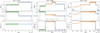Fig. A.1. Snapshots of the fiducial planar run (au = 2, Ek0,4=Ek0,1, ton,1:ton,4:toff = 1:1:1.) at t=t0 (left), before first shock crossing (center), and after shock crossing (right). Shells are color-coded according to the identified zones, the dashed lines show theoretical values. t0 = 2.7×103 s and R0 = 8×1013 cm for this set of parameters.

The values across the shocked region remain constant in time with very good accuracy compared to the analytical results: the proper speed, u, matches its expected value with a precision of the order 10⁻⁵, and derived quantities such as the shock strength Γ_ud−1 offers a match to within a few times 10⁻⁴. We also recover the analytical values for the shock crossing times t_RS and t_FS with an accuracy of 10⁻³, consistent with a systematic error of a few time steps due to the finite width of the numerical shock.

Appendix B: Flux calculation in the power-law approximation

B.1. Analytical flux

We present here the formalism for the analytical calculation of the flux received at observer time T and frequency ν from a range of emitting radii. From Eq. (4) we see that a single pulse emitted at a single time and radius in the source frame can be seen over a range of observed times. This means that several source times and radii contribute to a single observer time, defining a surface called equal arrival time surface (EATS) as the locus of all emission points from which photons will arrive at the same time to the observer. In R24b, itself expanding on previous works (e.g., Granot 2005; Granot et al. 2008; Genet & Granot 2009), the authors derive the observed flux coming from a shock front propagating with Lorentz factor Γ_sh=Γ_sh,0(R/R₀)^−m/2, emitting between radii R₀ and R_f=(1+ΔR/R₀)R₀ at a peak frequency ${\nu }_{\mathrm{p}}^{\prime }={\nu }_0^{\prime }(R/R_0{)}^d$ and with peak luminosity $L_{{\nu }_{\mathrm{p}}^{\prime }}^{\prime }=L_0^{\prime }(R/R_0{)}^a$. As quantities introduced in this subsection are relative to a single shock front, we have dropped the subscript RS (respectively FS) for the sake of readability. Additionally in R24, compared to GG09, it is the shocked material traveling with a Lorentz factor of Γ=gΓ_sh that is considered to be the source of emission. This means that while the shock front itself serves to determine the location of the emitting surface, it is the emitting material that will be considered for the Doppler factor.

The flux is calculated against normalized time $\tilde{T}$ defined as:

$$\tilde{T}=\frac{T-T_{\mathrm{ej},0}}{T_0}\hspace{0.5em},$$(B.1)

where T_ej,0 and T₀ are the effective (observed) ejection time and angular time as defined Eq. (5) for the shock front at R₀ the initial collision radius:

$$T_0=(1+z)\left(\frac{1-{\beta }_{\mathrm{sh},0}}{{\beta }_{\mathrm{sh},0}}\right)\frac{R_0}{c}\approx (1+z)\frac{R_0}{2c{\mathrm{\Gamma }}_{\mathrm{sh},0}^2}\hspace{0.5em},$$(B.2)

$$T_{\mathrm{ej},0}=(1+z)\left(t_0-\frac{R_0}{{\beta }_{\mathrm{sh},0}c}\right)\hspace{0.5em}.$$(B.3)

We do not provide here the details of the EATS and intermediate variables definitions, and instead refer again to appendix F of R24b for full details of the calculation. We introduce the normalized radius $y(\tilde{T})\equiv R/R_L(\tilde{T})$ and obtain the flux by integrating from y_min to y_max, defined as:

$$y_{\min }(\tilde{T})=\{\begin{array}{cc}1\hfill & \text{if}\hspace{0.5em}\tilde{T}\le 1\hspace{0.5em},\hfill \\ {\tilde{T}}^{-1/(m+1)}\hfill & \text{if}\hspace{0.5em}\tilde{T}\ge 1\hspace{0.5em},\hfill \end{array}$$(B.4)

$$y_{\max }(\tilde{T})=\{\begin{array}{cc}1\hfill & \text{if}\hspace{0.5em}{\tilde{T}}_f\le 1\hspace{0.5em},\hfill \\ {\tilde{T}}_f^{-1/(m+1)}\hfill & \text{if}\hspace{0.5em}{\tilde{T}}_f\ge 1\hspace{0.5em},\hfill \end{array}$$(B.5)

where ${\tilde{T}}_f=(1+\mathrm{\Delta }R/R_0{)}^{m+1}$. The Doppler factor is also expressed as a function of y:

$$\begin{array}{cc}\hfill \delta =(1+z)\frac{\nu }{{\nu }^{\prime }}=\frac{1+z}{\mathrm{\Gamma }(1-\beta \mu )}\approx (1+z)\frac{2(m+1)g{\mathrm{\Gamma }}_{\mathrm{sh},0}{y}^{\frac{m}{2}}{\tilde{T}}^{\frac{-m}{2(m+1)}}}{g^2{y}^{-1}+(m+1-g^2)y^m}\hspace{0.5em}.& \hfill \end{array}$$(B.6)

The received flux at normalized observer time $\tilde{T}$ for any given comoving luminosity $L_{{\nu }^{\prime }}^{\prime }(y)$ can be expressed as:

$$F_{\nu }(\tilde{T})=\frac{1+z}{8\pi d_L^2}{\displaystyle {\int }_{y_{\min }}^{y_{\max }}}\left|\frac{\mathrm{d}\mu }{\mathrm{d}y}\right|{\delta }^3{L}_{{\nu }^{\prime }}^{\prime }(y)\mathrm{d}y.$$(B.7)

With the change of variable:

$$\frac{\mathrm{d}\mu }{\mathrm{d}y}=\frac{y^{-2}(1+{\mathit{my}}^{m+1})}{2(m+1){\mathrm{\Gamma }}_{\mathrm{sh},0}^2}{\tilde{T}}^{m/(m+1)},$$(B.8)

and using Eq. (B.6) in B.7:

$$\begin{array}{cc}\hfill F_{\nu }(\tilde{T})=\frac{(1+z)g^3{\mathrm{\Gamma }}_{\mathrm{sh},0}{\tilde{T}}^{\frac{-m}{2(m+1)}}}{2\pi d_L^2}{\displaystyle {\int }_{y_{\min }}^{y_{\max }}}\mathrm{d}y{L}_{{\nu }^{\prime }}^{\prime }(y)y^{-1-\frac{m}{2}}\hspace{0.5em}& \hfill \\ \hfill \hspace{0.5em}\hspace{0.5em}\times {\left[1+g^2\frac{y^{-(m+1)}-1}{m+1}\right]}^{-2}\left(\frac{1+{\mathit{my}}^{m+1}}{g^2+(m+1-g^2)y^{m+1}}\right)\hspace{0.5em}.& \hfill \end{array}$$(B.9)

In the general case, we chose power-law scalings for the luminosity and peak frequency with radius:

$$L_{{\nu }^{\prime }}^{\prime }=L_0^{\prime }{\left(\frac{R}{R_0}\right)}^{a}S\left(\frac{{\nu }^{\prime }}{{\nu }_p^{\prime }}\right)=L_0^{\prime }{\tilde{T}}^a{y}^{a}S\left(\frac{{\nu }^{\prime }}{{\nu }_p^{\prime }}\right)\hspace{0.5em},$$(B.10)

$$\frac{{\nu }^{\prime }}{{\nu }_p^{\prime }}={\tilde{T}}^{-d}{y}^{m/2-d}\left[1+g^2\frac{(y^{-(m+1)}-1)}{m+1}\right]\frac{\nu }{{\nu }_0}\hspace{0.5em}.$$(B.11)

B.2. Numerical flux normalization

To obtain the appropriate flux from a numerical cell corresponding to the infinitely thin shell approximation used in R24b, we compare the isotropic energy obtained by integrating Eq. (4) with the equivalent integration of the flux formula from De Colle et al. (2012) for the contribution from a single computational cell, which for an isotropic comoving emissivity per unit volume and frequency, $P_{{\nu }^{\prime },\mathrm{jk}}^{\prime }$, reads:

$$\begin{array}{cc}\hfill & \mathrm{\Delta }{F}_{\nu ,\mathrm{ijk}}=\frac{(1+z{)}^2}{4\pi d_{\mathrm{L}}^2}\frac{\mathrm{\Delta }{V}_{\mathrm{ijk}}^{(4)}}{\mathrm{\Delta }{T}_{\mathrm{obs},\mathrm{i}}}\frac{P_{{\nu }^{\prime },\mathrm{jk}}^{\prime }}{{\mathrm{\Gamma }}_{\mathrm{jk}}^2(1-{\beta }_{\mathrm{jk}}cos{\theta }_{\mathrm{jk}}{)}^2}\hspace{0.5em},\hfill \\ \hfill & \text{for}\hspace{0.5em}\left|T_{\mathrm{obs},\mathrm{z},\mathrm{i}}-t_{\mathrm{jk}}+\frac{r_{\mathrm{jk}}cos{\theta }_{\mathrm{jk}}}{c}\right|<\frac{\mathrm{\Delta }{T}_{\mathrm{obs},\mathrm{z},\mathrm{i}}}{2}\hspace{0.5em}.\hfill \end{array}$$(B.12)

Here T_obs,z=T_obs/(1+z) and ν_z=(1+z)ν are measured in the source's cosmological frame, as is the (Lorentz invariant) 4-volume ΔV⁽⁴⁾. In this section, subscript i refer to observer time bins over which flux is calculated, subscript j to the simulation time step, and subscript k to the numerical cell within data file j. This approach attributes all of the contribution from any given numerical 4D cell jk to a single observer time interval i. This approximation relies on sufficiently fine spatial (and temporal) resolution and on the Doppler factor not significantly varying within the cell, due to the variation of its velocity direction with respect to the direction to the observer. However, our simulation is spatially 1D: the Doppler factor significantly varies within each numerical cell of lab-frame volume $\mathrm{\Delta }{V}_{\mathrm{jk}}^{(4)}=4\pi r^2\mathrm{\Delta }r$ and contributes to different observed time bins. We thus divide 1D cells further into subcells along the θ coordinate in which the Doppler factor can be considered constant.

The observed flux depends only on μ = cos θ through the Doppler factor and the photon arrival time but not on the ϕ coordinate as we calculate flux along the outflow axis. Thus each subdivision of volume $\mathrm{\Delta }{V}_{\mathrm{ijk}}^{(4)}=2\pi r_{\mathrm{jk}}^2\mathrm{\Delta }{r}_{\mathrm{jk}}\mathrm{\Delta }{\mu }_{\mathrm{i}}\mathrm{\Delta }{t}_{\mathrm{j}}$ contributes to the time bin centered on T_obs,i=(1+z)(t_j−r_jkμ_i/c) of width ΔT_obs,i=(1+z)(r_jk/c)Δμ_i. Recalling $E_{\mathrm{iso}}=\int d{\nu }_z\int {\mathit{dT}}_{\mathrm{obs},\mathrm{z}}{L}_{{\nu }_{\mathrm{z}},\mathrm{iso}}=\left(4\pi d_{\mathrm{L}}^2/(1+z)\right)\int {\mathit{dT}}_{\mathrm{obs}}\int d\nu F_{\nu }(T_{\mathrm{obs}})$, the isotropic energy for a spherical cell reads:

$$\begin{array}{cc}\hfill E_{\mathrm{iso},\mathrm{jk}}^{(\mathrm{num})}& =\frac{4\pi d_{\mathrm{L}}^2}{1+z}{\displaystyle \int }d\nu {\displaystyle \sum _{\mathrm{i}}}\mathrm{\Delta }{T}_{\mathrm{obs},\mathrm{i}}\mathrm{\Delta }{F}_{\nu ,\mathrm{ijk}}\hfill \\ \hfill & ={\displaystyle \int }d{\nu }_z{\displaystyle \sum _{\mathrm{i}}}\mathrm{\Delta }{V}_{\mathrm{ijk}}^{(4)}\frac{P_{{\nu }^{\prime },\mathrm{jk}}^{\prime }}{{\mathrm{\Gamma }}_{\mathrm{jk}}^2(1-{\beta }_{\mathrm{jk}}{\mu }_{\mathrm{i}}{)}^2}\hfill \\ \hfill & =2\pi r_{\mathrm{jk}}^2\mathrm{\Delta }{r}_{\mathrm{jk}}\mathrm{\Delta }{t}_{\mathrm{j}}\frac{P_{{\nu }_{\mathrm{m},\mathrm{jk}}^{\prime }}^{\prime }}{{\mathrm{\Gamma }}_{\mathrm{jk}}^2}{\displaystyle {\int }_0^{\infty }}d{\nu }_z{\displaystyle {\int }_{-1}^1}d\mu (1-\beta \mu {)}^{-2}S\left(\frac{{\nu }^{\prime }}{{\nu }_{\mathrm{m},\mathrm{jk}}^{\prime }}\right)\hfill \\ \hfill & =\mathrm{\Delta }{V}_{\mathrm{jk}}^{(4)}(1-{\beta }_{\mathrm{jk}}){\mathrm{\Gamma }}_{\mathrm{jk}}^2{\nu }_{\mathrm{m},\mathrm{z},\mathrm{jk}}{P}_{{\nu }_{\mathrm{m},\mathrm{jk}}^{\prime }}^{\prime }\mathcal{A}\cong \frac{1}{2}\mathrm{\Delta }{V}_{\mathrm{jk}}^{(4)}{\nu }_{\mathrm{m},\mathrm{z},\mathrm{jk}}{P}_{{\nu }_{\mathrm{m},\mathrm{jk}}^{\prime }}^{\prime }\mathcal{A}\hspace{0.5em},\hfill \end{array}$$(B.13)

having changed variables to $x\equiv {\nu }^{\prime }/{\nu }_{\mathrm{m}}^{\prime }=\nu (1-\beta \mu )/\left[{\nu }_{\mathrm{m}}(1-\beta )\right]={\nu }_z(1-\beta \mu )/\left[{\nu }_{\mathrm{m},\mathrm{z}}(1-\beta )\right]$ and denoting $\mathcal{A}=\int S(x)\mathrm{d}x$. In De Colle et al. (2012) the flux at a fixed observed time bin was calculated by summing over j and k. To obtain the isotropic energy we performed the opposite, namely, fixing j and k and summing over i (and integrated over frequency). Performing the equivalent integration on a single shell in the infinitely thin shell approximation (Genet & Granot 2009) is expressed as:

$$\begin{array}{cc}\hfill E_{\mathit{iso}}^{(\mathit{th})}& =\frac{4\pi d_{\mathrm{L}}^2}{1+z}{\displaystyle \int }{\mathit{dT}}_{\mathrm{obs}}{\displaystyle \int }d\nu F_{\nu }\hfill \\ \hfill & ={\tilde{L}}_{{\nu }_{\mathrm{m}}}{T}_{\theta }{\displaystyle \int }\frac{d\tilde{T}}{{\tilde{T}}^2}{\displaystyle \int }d\nu S\left(\frac{\nu }{{\nu }_{\mathrm{m}}}\tilde{T}\right)=\frac{1}{2}{\nu }_{\mathrm{m},\mathrm{z}}{\tilde{L}}_{{\nu }_{\mathrm{m},\mathrm{z}}}{T}_{\theta ,z}\mathcal{A}\hspace{0.5em},\hfill \end{array}$$(B.14)

using change of variable $x\equiv (\nu /{\nu }_{\mathrm{m}})\tilde{T}$. Finally, we obtain the equivalent numerical luminosity for simulation cell k of data file j in the infinitely thin shell approximation:

$${\tilde{L}}_{{\nu }_{\mathrm{m},\mathrm{z}},\mathrm{jk}}=\frac{\mathrm{\Delta }{V}_{\mathrm{jk}}^{(4)}{P}_{{\nu }_{\mathrm{m}}^{\prime },\mathrm{jk}}^{\prime }}{T_{\theta ,z,\mathrm{jk}}}=\frac{\mathrm{\Delta }{E}_{{\nu }_{\mathrm{m}}^{\prime },\mathrm{jk}}^{\prime }}{T_{\theta ,z,\mathrm{jk}}}\hspace{0.5em}.$$(B.15)

Here $\mathrm{\Delta }{E}_{{\nu }_{\mathrm{m}}^{\prime },\mathrm{jk}}^{\prime }$ is the energy emitted per unit frequency in the comoving frame by the four-dimensional cell jk. Going further with the infinitely thin shell approximation, we can assume all the energy given to the accelerated electrons is radiated over a time smaller than the numerical time step, and we write:

$${\tilde{L}}_{{\nu }_{\mathrm{m},\mathrm{z}},\mathrm{jk}}=\frac{{\mathrm{\Gamma }}_{\mathrm{jk}}\mathrm{\Delta }{V}_{\mathrm{jk}}^{(3)}{ϵ}_{\mathrm{e}}{e}_{\mathrm{jk}}^{\prime }}{W(p){\nu }_{\mathrm{m},\mathrm{jk}}^{\prime }{T}_{\theta ,z,\mathrm{jk}}}\hspace{0.5em}.$$(B.16)

B.3. Flux calibration

While the general analytical formula for any scaling indices a,d,m was not obtained and the integral in Eq. (B.9) must be calculated numerically, two special cases with a simpler integral form are of interest to us. We use the first case a,d,m = 0,0,0 to calibrate the post-processing methods in a consistent way from our fully planar simulation before extending them to the physically-relevant spherical geometry. With these simplifying assumptions, the observed flux is:

$$F_{\nu }(\tilde{T}\ge 1)=\frac{(1+z)g^3{\mathrm{\Gamma }}_{\mathrm{sh}}{L}_0^{\prime }}{2\pi d_{\mathrm{L}}^2}{\displaystyle {\int }_{y_{\min }}^{y_{\max }}}\frac{\mathrm{d}y{y}^{-2}S\left(x\right)}{{\left[1+g^2(y^{-1}-1)\right]}^3}\hspace{0.5em}.$$(B.17)

With

$$x=\frac{{\nu }^{\prime }}{{\nu }_0^{\prime }}=\left[1+g^2(y^{-1}-1)\right]\tilde{\nu }\hspace{0.5em},$$(B.18)

$$\tilde{\nu }=\nu /{\nu }_0\hspace{0.5em},$$(B.19)

$$\tilde{T}=\frac{T-T_{\mathrm{ej}}(R_0,{\beta }_{\mathrm{sh}})}{T_{\theta }(R_0,{\mathrm{\Gamma }}_{\mathrm{sh}})})\equiv 1+\overline{T}\hspace{0.5em},$$(B.20)

and the integration limits y_min, y_max are defined in Eqs. (B.4)-(B.5). Choosing x as the new integration variable, we obtain:

$$F_{\nu }=\frac{(1+z)2{\mathrm{\Gamma }}_0{L}_0^{\prime }}{4\pi d_{\mathrm{L}}^2}{\left(\frac{\nu }{{\nu }_0}\right)}^2{\displaystyle {\int }_{x_{\mathrm{l}}}^{x_{\mathrm{u}}}}\mathrm{d}x{x}^{-3}S(x).\hspace{0.5em}$$(B.21)

The upper and lower integration limits are, respectively, x_u=x(y_min) and x_l=x(y_max) and the integral is performed numerically using the quad method from scipy.odeint². We present in Fig. B.1 light curves at $\tilde{\nu }={10}^{-1}$ and instantaneous spectra at $\overline{T}=1$ obtained from our fiducial run in planar geometry, compared to the analytical flux obtained analytically with Eq. (B.21). The figure presents the observed flux using either the smooth Band function (top row) or a broken power-law (bottom row). Depending on the local spectral shape, the relative contributions of both shock to the light curve between their respective peak frequencies may vary, also causing a change in the peak flux at this intermediary frequency range, but the overall shape of the light curve obtained by the sum of both contributions do not. This difference between peak frequencies is better shown in the instantaneous spectrum where the shape of the curve between the peaks shows more variation with spectral shape. Our numerical fluxes agree with their analytical counterparts to a good degree of precision.

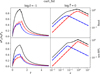Fig. B.1. Light curves (left column) and instantaneous spectra (right column) obtained from the fiducial run in planar geometry (full lines) compared to the analytical expectations (dash-dotted lines). Normalizations of $\overline{T}$ and $\tilde{\nu }$ are defined at the RS. The top row display the result for a Band spectral shape, and in the bottom the synchrotron broken power-law. The respective contributions of each shock to the total observed flux (in black) are given in red for the RS and blue for the FS.

Appendix C: The effective radius approximation

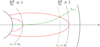Fig. C.1. Schematic representation of the effective radius approximation used to derive peak frequency and flux from the hydrodynamical data depending on the asymptotical regime. The EATS is shown in red.

All Tables

All Figures

	Fig. 1. Snapshots of the run in spherical geometry, with all parameters similar to the fiducial run, at t=t0 (left), before first (reverse) shock crossing (center), and after shock crossing (right). Dashed black lines show the analytical expectations from the results in planar geometry. The legend is the same for all panels.
In the text

Fig. 2. Top to bottom: comoving densities, Lorentz factors of the fluid and shock fronts, pressure, and shock strengths. The hydrodynamical quantities are measured downstream of shocks (‘d,3’ downstream of the RS, ‘d,2’ for the FS), at the CD by averaging over a few cells crossing the interface, or on each side of it (CD3, CD2) for the density. Legend is the same for all panels. The derived Lorentz factor of the shock fronts is displayed with the measured ones. Densities and pressures are in units of the values behind the RS in the planar case and rescaled to (r/R0)2. We smoothed the numerical oscillations in data by a rolling average. Horizontal dashed lines show the corresponding analytical values from R24a.

In the text

	Fig. 3. Top: Lorentz factors of the shock fronts, the fluid downstream of the shocks and at the CD with radius. Bottom: evolution of shock strengths with radius. Data were smoothed by rolling average. The quantities converge smoothly to a constant value after r≈4R0, shown by the dotted horizontal line for the quantities relative to the RS and the FS. Legend is the same as in Fig. 2.
In the text

Fig. 4. Light curves in the spherical (full lines) and hybrid (planar geometry and spherical assumptions for peak frequency and luminosity, dash-dotted lines) cases at fixed frequency $\tilde{\nu }=0.1$. Top panel: light curves with the Band's spectral shape. Bottom panel: broken power-law spectral shape. The total light curve in the hybrid + Band case is redrawn in the bottom panel (dotted line) for the sake of comparison. The individual contributions from each shock change but the resulting light curve do not, apart from the slightly increased breaks from the increase in crossing times. The choice of spectral shape decreases total emission at this frequency, while keeping the same time evolution.

In the text

Fig. 5. Time-integrated spectra following the same structure as in Fig. 4. The spherical effects decrease the peak frequencies for both shocks, with a stronger effect on the RS. The peaks from both contributions are closer than in the planar case, resulting in a three-part spectrum. This effect is more visible with the broken power-law spectral shape where the two peaks are distinct from each other in the hybrid approach. The choice for the spectral shape also diminishes the flux at low frequencies.

In the text

	Fig. 6. Normalized time evolution of peak frequency and flux for both shock fronts in the spherical (full line) and hybrid (dash-dotted) cases, calculated from the flux obtained with the Band spectral shape. In spherical geometry, the peak frequency decrease at a faster rate during the rising phase and the flux reaches saturation before the break to the high-latitude emission.
In the text

	Fig. 7. Left: νFν at peak frequency vs peak frequency for the reverse shock in the spherical and hybrid case. The fully spherical case show peak flux over a larger range of frequencies. Right: ratio between break frequency νbk and frequency at half flux ν1/2. Legend is the same for both panels.
In the text

	Fig. 8. Comparison of instantaneous spectra between two fast-cooling shock fronts (full lines) versus a fast-cooling RS and a marginally fast-cooling FS (dash-dotted lines) at $\overline{T}=1$. The low energy slopes are steeper and the overall flux is lower with a marginally fast-cooling FS.
In the text

	Fig. A.1. Snapshots of the fiducial planar run (au = 2, Ek0,4=Ek0,1, ton,1:ton,4:toff = 1:1:1.) at t=t0 (left), before first shock crossing (center), and after shock crossing (right). Shells are color-coded according to the identified zones, the dashed lines show theoretical values. t0 = 2.7×103 s and R0 = 8×1013 cm for this set of parameters.
In the text

Fig. B.1. Light curves (left column) and instantaneous spectra (right column) obtained from the fiducial run in planar geometry (full lines) compared to the analytical expectations (dash-dotted lines). Normalizations of $\overline{T}$ and $\tilde{\nu }$ are defined at the RS. The top row display the result for a Band spectral shape, and in the bottom the synchrotron broken power-law. The respective contributions of each shock to the total observed flux (in black) are given in red for the RS and blue for the FS.

In the text

	Fig. C.1. Schematic representation of the effective radius approximation used to derive peak frequency and flux from the hydrodynamical data depending on the asymptotical regime. The EATS is shown in red.
In the text

References

- Ayache, E. H., van Eerten, H. J., & Eardley, R. W. 2022, MNRAS, 510, 1315 [Google Scholar]
- Band, D., Matteson, J., Ford, L., et al. 1993, ApJ, 413, 281 [Google Scholar]
- Beloborodov, A. M. 2000, ApJ, 539, L25 [Google Scholar]
- Bošnjak, Ž., & Daigne, F. 2014, A&A, 568, A45 [NASA ADS] [CrossRef] [EDP Sciences] [Google Scholar]
- Bošnjak, Ž., Daigne, F., & Dubus, G. 2009, A&A, 498, 677 [NASA ADS] [CrossRef] [EDP Sciences] [Google Scholar]
- Burgess, J. M., Preece, R. D., Connaughton, V., et al. 2014, ApJ, 784, 17 [NASA ADS] [CrossRef] [Google Scholar]
- Bustamante, M., Heinze, J., Murase, K., & Winter, W. 2017, ApJ, 837, 33 [NASA ADS] [CrossRef] [Google Scholar]
- Courant, R., Friedrichs, K., & Lewy, H. 1928, Mathematische Annalen, 100, 32 [CrossRef] [Google Scholar]
- Daigne, F., & Mochkovitch, R. 1998, MNRAS, 296, 275 [NASA ADS] [CrossRef] [Google Scholar]
- De Colle, F., Granot, J., López-Cámara, D., & Ramirez-Ruiz, E. 2012, ApJ, 746, 122 [NASA ADS] [CrossRef] [Google Scholar]
- Duffell, P. C., & MacFadyen, A. I. 2013, ApJ, 775, 87 [Google Scholar]
- Genet, F., & Granot, J. 2009, MNRAS, 399, 1328 [NASA ADS] [CrossRef] [Google Scholar]
- Granot, J. 2005, ApJ, 631, 1022 [Google Scholar]
- Granot, J., Cohen-Tanugi, J., & Silva, E. C. 2008, ApJ, 677, 92 [NASA ADS] [CrossRef] [Google Scholar]
- Guetta, D., Spada, M., & Waxman, E. 2001, ApJ, 557, 399 [NASA ADS] [CrossRef] [Google Scholar]
- Harten, A., Lax, P. D., & Leer, B. v., 1983, SIAM Review, 25, 35 [CrossRef] [Google Scholar]
- Jacovich, T. E., Beniamini, P., & van der Horst, A. J. 2021, MNRAS, 504, 528 [CrossRef] [Google Scholar]
- Kaiser, C. R., Sunyaev, R., & Spruit, H. C. 2000, A&A, 356, 975 [NASA ADS] [Google Scholar]
- Kino, M., Mizuta, A., & Yamada, S. 2004, ApJ, 611, 1021 [Google Scholar]
- Kobayashi, S., Piran, T., & Sari, R. 1997, ApJ, 490, 92 [Google Scholar]
- Kumar, P., & Granot, J. 2003, ApJ, 591, 1075 [CrossRef] [Google Scholar]
- Malzac, J. 2014, MNRAS, 443, 299 [NASA ADS] [CrossRef] [Google Scholar]
- Mathews, W. G. 1971, ApJ, 165, 147 [Google Scholar]
- McCarthy, G. A., & Laskar, T. 2024, ApJ, 970, 135 [Google Scholar]
- Mignone, A., & Bodo, G. 2005, MNRAS, 364, 126 [Google Scholar]
- Mignone, A., & McKinney, J. C. 2007, MNRAS, 378, 1118 [Google Scholar]
- Nakar, E., & Piran, T. 2002, MNRAS, 331, 40 [NASA ADS] [CrossRef] [Google Scholar]
- Nakar, E., Ando, S., & Sari, R. 2009, ApJ, 703, 675 [NASA ADS] [CrossRef] [Google Scholar]
- Oganesyan, G., Nava, L., Ghirlanda, G., & Celotti, A. 2017, ApJ, 846, 137 [Google Scholar]
- Pe’er, A. 2014, Space Sci. Rev., 183, 371 [Google Scholar]
- Pe’er, A., Long, K., & Casella, P. 2017, ApJ, 846, 54 [Google Scholar]
- Pellouin, C., & Daigne, F. 2024, A&A, 690, A281 [NASA ADS] [CrossRef] [EDP Sciences] [Google Scholar]
- Preece, R., Burgess, J. M., Von Kienlin, A., et al. 2014, Science, 343, 51 [Google Scholar]
- Rahaman, S. M., Granot, J., & Beniamini, P. 2024a, MNRAS, 528, 160 [Google Scholar]
- Rahaman, S. M., Granot, J., & Beniamini, P. 2024b, MNRAS, 528, L45 [Google Scholar]
- Ravasio, M., Ghirlanda, G., Nava, L., & Ghisellini, G. 2019, A&A, 625, A60 [NASA ADS] [CrossRef] [EDP Sciences] [Google Scholar]
- Rees, M. 1978, MNRAS, 184, 61P [NASA ADS] [CrossRef] [Google Scholar]
- Rees, M. J., & Mészáros, P. 1994, ApJ, 430, L93 [Google Scholar]
- Rudolph, A., Bošnjak, Ž., Palladino, A., Sadeh, I., & Winter, W. 2022, MNRAS, 511, 5823 [Google Scholar]
- Rudolph, A., Petropoulou, M., Bošnjak, Ž., & Winter, W. 2023, ApJ, 950, 28 [NASA ADS] [CrossRef] [Google Scholar]
- Sari, R., & Piran, T. 1997, MNRAS, 287, 110 [Google Scholar]
- Spada, M., Ghisellini, G., Lazzati, D., & Celotti, A. 2001, MNRAS, 325, 1559 [NASA ADS] [CrossRef] [Google Scholar]
- Spada, M., Panaitescu, A., & Meszaros, P. 2000, ApJ, 537, 824 [Google Scholar]
- Vianello, G., Gill, R., Granot, J., et al. 2018, ApJ, 864, 163 [NASA ADS] [CrossRef] [Google Scholar]
- Yan, Z. -Y., Yang, J., Zhao, X. -H., Meng, Y. -Z., & Zhang, B. -B. 2024, ApJ, 962, 85 [NASA ADS] [CrossRef] [Google Scholar]
- Zanotti, O., Rezzolla, L., Del Zanna, L., & Palenzuela, C. 2010, A&A, 523, A8 [NASA ADS] [CrossRef] [EDP Sciences] [Google Scholar]