| Issue |
A&A
Volume 699, July 2025
|
|
|---|---|---|
| Article Number | A271 | |
| Number of page(s) | 13 | |
| Section | Numerical methods and codes | |
| DOI | https://doi.org/10.1051/0004-6361/202453212 | |
| Published online | 16 July 2025 | |
Probabilistic estimators of Lagrangian shape biases: Universal relations and physical insights
1
Donostia International Physics Center,
Manuel Lardizabal Ibilbidea, 4,
20018
Donostia, Gipuzkoa,
Spain
2
Euskal Herriko Unibertsitatea, Edificio Ignacio Maria Barriola,
Plaza Elhuyar, 1,
20018
Donostia-San Sebastián,
Spain
3
Department of Astrophysics, University of Vienna,
Türkenschanzstraße 17,
1180
Vienna,
Austria
4
IKERBASQUE, Basque Foundation for Science,
48013
Bilbao,
Spain
★ Corresponding author.
Received:
28
November
2024
Accepted:
16
June
2025
Abstract
The intrinsic alignment of galaxies can provide valuable information for cosmological and astrophysical studies and is crucial for interpreting weak-lensing observations. Modeling intrinsic alignments requires understanding how galaxies acquire their shapes in relation to the large-scale gravitational field, which is typically encoded in the value of large-scale shape-bias parameters. In this article we contribute to this topic in three ways: (i) developing new estimators of Lagrangian shape biases, (ii) applying them to measure the shape biases of dark-matter halos, and (iii) interpreting these measurements to gain insight into the process of halo-shape formation. Our estimators yield measurements consistent with previous literature values and offer advantages over earlier methods; for example, our bias measurements are independent of other bias parameters, and we can define bias parameters for each individual object. We measure universal relations between shape-bias parameters and peak height, ν. For the first-order shape-bias parameter, this relation is close to linear at high ν and approaches zero at low ν, which provides evidence against the proposed scenario that galaxy shapes arise due to post-formation interaction with the large-scale tidal field. We anticipate that our estimators will be very useful for analyzing hydrodynamical simulations, and thereby enhance our understanding of galaxy shape formation, and for establishing priors on the values of intrinsic alignment biases.
Key words: galaxies: structure / cosmology: theory / large-scale structure of Universe
© The Authors 2025
 Open Access article, published by EDP Sciences, under the terms of the Creative Commons Attribution License (https://creativecommons.org/licenses/by/4.0), which permits unrestricted use, distribution, and reproduction in any medium, provided the original work is properly cited.
This article is published in open access under the Subscribe to Open model. This email address is being protected from spambots. You need JavaScript enabled to view it. to support open access publication.
1 Introduction
Cosmic shear (CS) is arguably the most direct way to probe the fluctuations of the matter field on cosmological scales (Mandelbaum 2018). The slight deformations to the baseline shapes of galaxies are not affected by the clustering properties of those galaxies, making these measurements independent of galaxy bias. As a result, the information on the amplitude of matter fluctuations, σ8, that can be extracted does not have the typical degeneracy with linear galaxy bias. However, an outstanding issue is that the shapes of galaxies before shearing are not entirely random but may be correlated with the large-scale gravitational field. Typically known as galaxy intrinsic alignments (IAs), this effect is highly dependent on galaxy-formation physics and contaminates CS measurements (Joachimi et al. 2015; Kiessling et al. 2015; Kirk et al. 2015; Troxel & Ishak 2015). Therefore, extracting reliable information from CS requires accurate modeling of IAs (Secco et al. 2022; Aricò et al. 2023; Preston et al. 2024).
Intrinsic alignment modeling is often based on a perturbative expansion (Desjacques et al. 2018). Early works modeled galaxy shapes as being linearly correlated to the large-scale tidal field, with the linear-alignment parameter (cK) left free to describe any galaxy population (Catelan et al. 2001; Hirata & Seljak 2004). In recent years, this field has seen many advancements, with the formulation of models that include higher orders in perturbation theory (Blazek et al. 2015), complete formulations using the effective field theory of large-scale structures both in Eulerian Vlah et al. 2020, 2021; Bakx et al. 2023) and Lagrangian (Chen & Kokron 2024) space, and hybrid prescriptions that use a bias expansion combined with the results of N-body simulations to produce models that extend accurately into the nonlinear regime (Maion et al. 2024). An integral part of all of these models is the “shape bias” parameters – free coefficients that encode the average response of a galaxy’s shape to the large-scale properties of the matter field.
Although the bias parameters of a certain population of objects cannot be easily predicted a priori, measuring their values can shed light on the formation mechanism of said objects. As an example, the detection of nonzero halo assembly bias for density bias parameters (Gao et al. 2005; Wechsler et al. 2006; Gao & White 2007; Angulo et al. 2008) has shown that dependences on halos’ accretion histories have to be included in predictions from excursion-set theory (Bardeen et al. 1986; Bond et al. 1991; Lacey & Cole 1993) to be in agreement with halo-bias measurements from N-body simulations (Dalal et al. 2008). Furthermore, it explained why simple halo occupation distribution models, which assume the galaxy content of a halo depends solely on its mass (Zheng et al. 2005), are inadequate in describing realistic measurements from simulations and galaxy surveys (Croton et al. 2007; Zehavi et al. 2018; Contreras et al. 2024). Measurements of shape biases are still in their infancy but should contribute similarly to the understanding of shape formation as they advance into a more mature stage.
A significant amount of research has been carried out to analyze the IAs of halos and galaxies, in both gravity-only and hydrodynamical simulations (Tenneti et al. 2014, 2015b,a, 2016, 2020; Chisari et al. 2015; Velliscig et al. 2015; Hilbert et al. 2017; Delgado et al. 2023), but with little focus on large-scale shape-bias parameters. The first direct measurements of shape bias parameters of simulated halos were performed by Stücker et al. (2021) and Akitsu et al. (2021) employing the “anisotropic separate universe” technique (Schmidt et al. 2018; Wagner et al. 2014). In a later work, Akitsu et al. (2023) employed the quadratic bias technique (Schmittfull et al. 2015) to measure second-order shape biases. These works have shown that there is a power-law scaling of the linear shape bias with halo mass and demonstrated its dependence on concentration for high-mass halos. A universal relation between the linear shape bias and b1, the linear density bias, was also established. Furthermore, they have quantified the dependence of second-order shape-bias parameters with halo mass and studied their dependence on b1. Nevertheless, many interesting questions remain unanswered.
The precise origin of halo-shape alignments with the large-scale gravitational field is still poorly understood. In one possible scenario, the large-scale gravitational forces progressively deform halos after their formation, producing an alignment that grows over time. Another possibility is that the shape is already encoded during the formation of halos – for example through the anisotropy of infall velocities as determined by the large-scale gravitational potential. It should be possible to distinguish between these scenarios through measurements of the bias parameters. Beyond this, it is important to understand how alignments depend quantitatively on the (often arbitrary) boundary definition of the considered system and whether the alignment strength is affected by secondary properties beyond halo mass – such as the spin or formation time.
While studies of halos in gravity-only simulations may provide a qualitative understanding of necessary model ingredients, the ultimate goal of theoretical alignment studies is an understanding of the shape biases of galaxies. Determining these values in realistic scenarios, such as high-resolution hydrodynamical simulations, would be a great advancement toward obtaining informative priors that could be applied to IA models in weak-lensing analyses (Zennaro et al. 2022; Ivanov et al. 2025; Ivanov et al. 2024; Shiferaw et al. 2024; Zhang et al. 2024). Additionally, the comparison of measurements of galaxy shape bias parameters obtained from hydrodynamical simulations to those measured from observations could be used as a way to constrain “subgrid” models of galaxy formation. To answer all these questions, we need a fast and precise estimator of shape biases.
In this manuscript, we generalize the theoretical formalism presented in Stücker et al. (2025) to develop estimators of shape biases. The estimators are based on measurements of correlations in the joint probability distribution of Lagrangian large-scale tides and the shape of a given object. Similar to the separate universe (SU) approach, this yields simple and robust measurements of these biases but with the additional benefit of low computational costs, making the method viable for use in large hydrodynamical simulations. We validate the estimators through convergence tests and a comparison with literature results. Finally, we provide detailed measurements of the shape biases of halos and discuss the theoretical implications for the modeling of IAs.
The article is structured as follows. In Sect. 2, we derive the new estimators based on considerations from probability theory. In Sect. 3, we present the set of simulations we used to validate our results. In Sect. 4, we test the robustness of our shape bias measurements and provide accurate fitting formulae. Finally, in Sect. 5 we summarize our findings and discuss future applications.
2 Probabilistic bias
Considering an object composed of a finite set of particles, N, one can define its shape tensor, 𝓘. This quantity is a rank-2 tensor, generally defined as
![Mathematical equation: $\[\mathcal{I}_{i j}=\frac{1}{N} \sum_{n=1}^N\left(x_i^{(n)}-\bar{x}_i\right)\left(x_j^{(n)}-\bar{x}_j\right),\]$](/articles/aa/full_html/2025/07/aa53212-24/aa53212-24-eq1.png) (1)
(1)
with the corresponding reduced shape tensor
![Mathematical equation: $\[\tilde{I}_{i j}=\frac{1}{N} \sum_{n=1}^N \frac{\left(x_i^{(n)}-\bar{x}_i\right)\left(x_j^{(n)}-\bar{x}_j\right)}{r_n^2},\]$](/articles/aa/full_html/2025/07/aa53212-24/aa53212-24-eq2.png) (2)
(2)
where ![Mathematical equation: $\[x_{i}^{(n)}\]$](/articles/aa/full_html/2025/07/aa53212-24/aa53212-24-eq3.png) represents the Eulerian position of each particle, n is an index running over the particles in the set, and i runs over the three Cartesian coordinates,
represents the Eulerian position of each particle, n is an index running over the particles in the set, and i runs over the three Cartesian coordinates, ![Mathematical equation: $\[\bar{x}_{i}\]$](/articles/aa/full_html/2025/07/aa53212-24/aa53212-24-eq4.png) is the mean of
is the mean of ![Mathematical equation: $\[x_{i}^{(n)}\]$](/articles/aa/full_html/2025/07/aa53212-24/aa53212-24-eq5.png) , and
, and ![Mathematical equation: $\[r_{n}^{2} \equiv {\sum}_{i}\left(x_{i}^{(n)}-\bar{x}_{i}\right)^{2}\]$](/articles/aa/full_html/2025/07/aa53212-24/aa53212-24-eq6.png) . We used the non-reduced shape definition for all results in this article, except when comparing different definitions.
. We used the non-reduced shape definition for all results in this article, except when comparing different definitions.
Now, we can define the normalized and trace-free part of ℐ:
![Mathematical equation: $\[I_{i j}(\mathbf{x})=\frac{\mathcal{T}_{i j}(\mathbf{x})}{\mathcal{I}_0}-\frac{1}{3} \delta_{i j}^K,\]$](/articles/aa/full_html/2025/07/aa53212-24/aa53212-24-eq7.png) (3)
(3)
in which ℐ0 is the trace of ℐij, and ![Mathematical equation: $\[\delta_{i j}^{K}\]$](/articles/aa/full_html/2025/07/aa53212-24/aa53212-24-eq8.png) is the Kronecker delta symbol.
is the Kronecker delta symbol.
The tensor I describes the shape of an object, factoring out its physical size. Being a symmetric tensor, it can be diagonalized to give three eigenvalues, I1,2,3, such that ![Mathematical equation: $\[{\sum}_{i=1}^{3} I_{i}=0\]$](/articles/aa/full_html/2025/07/aa53212-24/aa53212-24-eq9.png) . Each of these measures the relative extension of the object in each direction of an orthogonal basis formed by its eigenvectors. The goal of this work is to understand the response of this shape to changes in the large-scale gravitational field.
. Each of these measures the relative extension of the object in each direction of an orthogonal basis formed by its eigenvectors. The goal of this work is to understand the response of this shape to changes in the large-scale gravitational field.
Attempting to determine which large-scale properties could generate an effect, we find that the simplest object we can build, allowed by the equivalence principle and symmetry of the problem, is the Lagrangian tidal field:
![Mathematical equation: $\[T_{i j}(\mathbf{q})=\partial_i \partial_j \Phi_G(\mathbf{q}),\]$](/articles/aa/full_html/2025/07/aa53212-24/aa53212-24-eq10.png) (4)
(4)
where ΦG is the displacement potential, q is a position in Lagrangian coordinates, and the derivatives are taken with respect to this coordinate system. For convenience, we also defined the traceless part of the tidal field:
![Mathematical equation: $\[K_{i j}(\mathbf{q})=\left(\partial_i \partial_j-\frac{1}{3} \delta_{i j}^K\right) \Phi_G.\]$](/articles/aa/full_html/2025/07/aa53212-24/aa53212-24-eq11.png) (5)
(5)
Assuming for now that the tidal field is the only property of the Lagrangian matter field affecting the shapes of gravitationally bound objects, we can now develop a theoretical framework to quantify its effect.
A key assumption of the forthcoming calculations is the validity of the peak-background split (PBS; Bardeen et al. 1986). That is, we assumed that the criterion for forming a halo is defined relative to small-scale quantities; large scales only affect this process by introducing modulations to the distribution of small-scale perturbations. SU simulations provide an exact implementation of this scenario (Gnedin et al. 2011; Wagner et al. 2014; Schmidt et al. 2018; Stücker et al. 2021; Akitsu et al. 2021), and it is interesting to consider them for a moment.
Consider a simulation where a constant perturbation, T0, to the tidal field is introduced. Upon identifying a set of objects (e.g., halos or galaxies) in these simulations, one can compute their average shape as a function of the large-scale tide T0 (see Figure 1 for an illustration of this procedure). This yields a functional relation ⟨I|T0⟩g – where our notation indicates an expectation value that has been conditioned on T0 and that has been taken over galaxies (or halos). This function can be expanded in a perturbative series,
![Mathematical equation: $\[\left\langle\mathbf{I} {\mid} \mathbf{T}_0\right\rangle_g=\mathbf{C}_{K, 1} \mathbf{T}_0+\mathbf{T}_0^T \mathbf{C}_{K, 2} \mathbf{T}_0+\cdots,\]$](/articles/aa/full_html/2025/07/aa53212-24/aa53212-24-eq12.png) (6)
(6)
where CK,1 is a rank 2 tensor, CK,2 is of rank 4 and each product corresponds to a contraction over two indices. Therefore, by running SU simulations at several values of T0, one can compute derivatives of ⟨I|T0⟩ and, hence, extract generalized tensorial bias parameters:
![Mathematical equation: $\[\mathbf{C}_{K, n}=\left.\frac{\partial^n\left\langle\mathbf{I} {\mid} \mathbf{T}_0\right\rangle}{\partial \mathbf{T}_0^n}\right|_{\mathbf{T}_0=0}.\]$](/articles/aa/full_html/2025/07/aa53212-24/aa53212-24-eq13.png) (7)
(7)
SU simulations therefore provide a well-defined route to compute shape bias parameters. Unfortunately, they have the down-side of being costly due to the need to run several simulations at different values of T0. We now show an alternative route to measuring these bias parameters that is fully consistent with the SU method, using quantities that can be obtained from only a single simulation.
We began by considering the linear field of a simulation in a finite volume, smoothed with a sharp filter in k-space such that only modes with k < kd are retained. This linear field is characterized at first order by its tidal field, which we denote as T.
If we average the shape of galaxies that inhabit regions of the same tidal field T, we obtain the conditional expectation value ⟨I|T⟩g. Note that this function is slightly different than ⟨I|T0⟩g, since the tidal field measured at the finite scale kd carries a different amount of information than the idealized infinite scale field T0. However, using probability theory, we can emulate a change in the field at infinite scales, which modifies the distribution of the field at finite scales.
First of all, consider that if we have an expectation value of some variable h that is conditioned on two probability variables ⟨h|x, y⟩, then we can obtain the expectation value that is only conditioned on the variable x through a weighted average as
![Mathematical equation: $\[\langle h {\mid} x\rangle=\frac{\int\langle h {\mid} x, y\rangle p(y {\mid} x) \mathrm{d} y}{\int p(y {\mid} x) \mathrm{d} y},\]$](/articles/aa/full_html/2025/07/aa53212-24/aa53212-24-eq14.png) (8)
(8)
where the denominator can be omitted if p(y|x) is a normalized distribution. Additionally, we need to consider that the distribution of interest is not the (Gaussian) conditional distribution at random locations – let us refer to it as p(T|T0) – but instead it is the distribution at the locations of galaxies pg(T|T0). The two are related through a bias function:
![Mathematical equation: $\[p_g\left(\mathbf{T} {\mid} \mathbf{T}_0\right)=f\left(\mathbf{T}, \mathbf{T}_0\right) p\left(\mathbf{T} {\mid} \mathbf{T}_0\right),\]$](/articles/aa/full_html/2025/07/aa53212-24/aa53212-24-eq15.png) (9)
(9)
where f(T, T0) describes the relative excess probability of finding a galaxy in a region that has the tidal field T at finite scales and T0 at infinite scales (see Stücker et al. 2025, for a detailed explanation),
![Mathematical equation: $\[f\left(\mathbf{T}, \mathbf{T}_0\right)=\frac{p\left(g {\mid} \mathbf{T}, \mathbf{T}_0\right)}{p(g)},\]$](/articles/aa/full_html/2025/07/aa53212-24/aa53212-24-eq16.png) (10)
(10)
or, through Bayes’ theorem,
![Mathematical equation: $\[f\left(\mathbf{T}, \mathbf{T}_0\right)=\frac{p\left(\mathbf{T}, \mathbf{T}_0 {\mid} g\right)}{p\left(\mathbf{T}, \mathbf{T}_0\right)}.\]$](/articles/aa/full_html/2025/07/aa53212-24/aa53212-24-eq17.png) (11)
(11)
Under the PBS assumption the value of T0 is irrelevant if the smaller scale field T is known, so that f(T, T0) = f(T). Putting things together, we find
![Mathematical equation: $\[\left\langle\mathbf{I} {\mid} \mathbf{T}_0\right\rangle_g=\frac{\int\left\langle\mathbf{I} {\mid} \mathbf{T}_0, \mathbf{T}\right\rangle_g f(\mathbf{T}) p\left(\mathbf{T} {\mid} \mathbf{T}_0\right) d \mathbf{T}}{\int f(\mathbf{T}) p\left(\mathbf{T} {\mid} \mathbf{T}_0\right) d \mathbf{T}}.\]$](/articles/aa/full_html/2025/07/aa53212-24/aa53212-24-eq18.png) (12)
(12)
We can further simplify this expression by using that, under the PBS assumption, ⟨I|T0, T⟩g = ⟨I|T⟩g. Further, we defined the “renormalized bias function”:
![Mathematical equation: $\[\begin{aligned}F\left(\mathbf{T}_0\right) & =\int f(\mathbf{T}) p\left(\mathbf{T} {\mid} \mathbf{T}_0\right) d \mathbf{T} \\& =\left\langle f\left(\mathbf{T}+\mathbf{T}_0\right)\right\rangle,\end{aligned}\]$](/articles/aa/full_html/2025/07/aa53212-24/aa53212-24-eq19.png) (13)
(13)
where the second line assumes the use of a sharp k-space filter to define T (Stücker et al. 2025). We then find
![Mathematical equation: $\[\left\langle\mathbf{I} {\mid} \mathbf{T}_0\right\rangle_g=\frac{1}{F\left(\mathbf{T}_0\right)} \int\langle\mathbf{I} {\mid} \mathbf{T}\rangle_g f(\mathbf{T}) p\left(\mathbf{T} {\mid} \mathbf{T}_0\right) d \mathbf{T}\]$](/articles/aa/full_html/2025/07/aa53212-24/aa53212-24-eq20.png) (14)
(14)
![Mathematical equation: $\[=\frac{1}{F\left(\mathbf{T}_0\right)} \int\int \mathbf{I} \frac{p(\mathbf{I}, \mathbf{T} {\mid} g)}{p(\mathbf{T} {\mid} g)} f(\mathbf{T}) p\left(\mathbf{T} {\mid} \mathbf{T}_0\right) d \mathbf{I} d \mathbf{T}\]$](/articles/aa/full_html/2025/07/aa53212-24/aa53212-24-eq21.png) (15)
(15)
![Mathematical equation: $\[=\frac{1}{F\left(\mathbf{T}_0\right)} \int\int \mathbf{I} p(\mathbf{I}, \mathbf{T} {\mid} g) \frac{p\left(\mathbf{T} {\mid} \mathbf{T}_0\right)}{p(\mathbf{T})} d \mathbf{I} d \mathbf{T}\]$](/articles/aa/full_html/2025/07/aa53212-24/aa53212-24-eq22.png) (16)
(16)
![Mathematical equation: $\[=\frac{1}{F\left(\mathbf{T}_0\right)}\left\langle\mathbf{I} \frac{p\left(\mathbf{T} {\mid} \mathbf{T}_0\right)}{p(\mathbf{T})}\right\rangle_g,\]$](/articles/aa/full_html/2025/07/aa53212-24/aa53212-24-eq23.png) (17)
(17)
where in the second line we have expanded ⟨I|T⟩g as an integral, in the third line we used Bayes’ theorem f(T) = p(g|T)/ p(g) = p(T|g) /p(T), and we rewrote the double integral over I and T weighted by p(I, T|g) as an average over all galaxies. Equation (17) simply tells us that one can recover the SU average ⟨I|T0⟩g by calculating the weighted average of shapes – where the weight corresponds to the relative increase in the probability of finding each galaxy’s environment if a large-scale tidal field T0 is applied.
For the case of a sharp k-space filter, it is p(T|T0) = p(T − T0) so that after substituting into Eq. (7) we find
![Mathematical equation: $\[\mathbf{C}_{K, 1}=\left\langle\frac{1}{p(\mathbf{T})} \mathbf{I} \otimes\left(-\mathbf{p}^{(1)}(\mathbf{T})-p \mathbf{F}^{(1)}(0)\right)\right\rangle_g\]$](/articles/aa/full_html/2025/07/aa53212-24/aa53212-24-eq24.png) (18)
(18)
![Mathematical equation: $\[\mathbf{C}_{K, 2}=\left\langle\frac{1}{p(\mathbf{T})} \mathbf{I} \otimes\left(\mathbf{p}^{(2)}+2 \mathbf{p}^{(1)} \otimes \mathbf{F}^{(1)}-p \mathbf{F}^{(2)}+p\left(\mathbf{F}^{(1)}\right)^2\right)\right\rangle_g,\]$](/articles/aa/full_html/2025/07/aa53212-24/aa53212-24-eq25.png) (19)
(19)
where we write the derivatives with respect to T in boldface to remark that this derivative is a 2k-rank tensor in which k is the order of the derivative.
The procedure outlined in this section defines an estimator of the shape biases, which we show to be unbiased and which has some notable properties:
It can be defined on an object-by-object basis, by evaluating Eq. (18) without the averaging brackets.
This estimator does not rely on the calculation of n-point functions, making it simpler to evaluate for any selection of objects, even in complex geometries.
The re-normalization procedure is conceptually very simple in this picture.
Let us expand a bit more on this final point. When measuring bias parameters using n-point functions computed with perturbation theory, an issue appears that these measurements depend on the cutoff scale, Λ, used to divide large-from and small-scale modes (see Assassi et al. 2014; Desjacques et al. 2018; and Rubira & Schmidt 2024 for a detailed explanation). Similarly, our individual bias estimates also depend on the scale at which we damped our density field, kd. However, after we average those estimates weighted by the probability density function (PDF) of the matter perturbations, this dependence should be approximately removed. This procedure should work well as long as it is a good approximation that the distribution of Tij is a multivariate Gaussian, and that its cross-correlations with other observables are small. An issue appears of course when we make kd similar to 1/R*, where we denote by R* the typical Lagrangian scale of halos. At these scales, higher-derivative operators become relevant, and one needs to consider their cross-correlation with Tij to properly estimate the values of bias-parameters.
The properties mentioned above are also present in the estimators derived in the following sections of this manuscript.
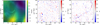 |
Fig. 1 Illustration of halo shapes in a simulation slice and their relation to the underlying density and tidal fields. Left: density field linearly extrapolated to z = 0 (background), with a large set of small arrows superimposed. The sizes of these small arrows are scaled to the local projected tidal field’s largest eigenvalue, and their direction is that of the corresponding eigenvector. Middle: halos (colored ellipses) centered at their Lagrangian positions. Their shapes are those of the projected shape tensor estimated for the FoF group; their color corresponds to the value of their three-dimensional shape-alignment bias. Right: same as the middle panel except now the halos are at their final Eulerian positions. |
2.1 Linear bias
The derivation leading to Eq. (18) has been left so far in a very general form; we now connect it to more common definitions of shape biases found in the literature.
From Eq. (7) taken at n = 1, we can see that the values assumed by the rank-4 tensor CK,1 are constrained by the symmetries of the right-hand side, that is, CK,1 has to be isotropic, symmetric over its first two indices (given the symmetry of ⟨I|T0⟩) and the last two as well (given the symmetry of T). In Appendix B we summarize the findings of Stücker et al. (2025), who derived an orthogonal basis for all isotropic rank-4 tensors that respect the imposed symmetries, 𝕍22 = span({J22, J2=2}), in which the tensors J22 and J2=2 are defined by
![Mathematical equation: $\[\mathbf{J}_{22}=S_{22}\left(\delta_{i j}^K \delta_{k l}^K\right)\]$](/articles/aa/full_html/2025/07/aa53212-24/aa53212-24-eq26.png) (20)
(20)
![Mathematical equation: $\[\mathbf{J}_{2=2}=S_{22}\left(\delta_{i k}^K \delta_{j l}^K\right)-\frac{1}{3} S_{22}\left(\delta_{i j}^K \delta_{k l}^K\right),\]$](/articles/aa/full_html/2025/07/aa53212-24/aa53212-24-eq27.png) (21)
(21)
where S22 is a double symmetrization operator, defined via its action on an arbitrary rank-4 tensor M, given by
![Mathematical equation: $\[S_{22}\left(M_{i j k l}\right)=\frac{1}{4}\left(M_{i j k l}+M_{j i k l}+M_{i j l k}+M_{j i l k}\right).\]$](/articles/aa/full_html/2025/07/aa53212-24/aa53212-24-eq28.png) (22)
(22)
It is useful to keep in mind that the notation we employ gives information on the result of contracting these tensors with any arbitrary rank-2 tensors A and B. Contracting J22 with A and B simply gives us the product of their traces – each subscript “2” without any connection symbol represents taking the trace of a rank-2 tensor. As for J2=2, contracting it with A and B gives the trace of their matrix product; each “–” symbol connecting the subscripts represents summation over one repeated index; in this case, the first one is due to the matrix product, and a second one must appear to form the trace of this product.
Using this basis, one can uniquely decompose CK,1 as a linear combination,
![Mathematical equation: $\[\mathbf{C}_{K, 1}=c_{J_{22}} \mathbf{J}_{22}+c_{J_{2=2}} \mathbf{J}_{2=2},\]$](/articles/aa/full_html/2025/07/aa53212-24/aa53212-24-eq29.png) (23)
(23)
and, by contracting with the basis tensors and taking advantage of orthogonality, we can write the expressions for the bias parameters in Eq. (32),
![Mathematical equation: $\[c_{J_{22}}=-\left\langle\frac{1}{p(\mathbf{T})}\left(\frac{\partial p}{\partial \mathbf{T}}-p \frac{\partial F}{\partial \mathbf{T}}(0)\right) \otimes \mathbf{I}^{(4)}_{~~~\cdot} \frac{\mathbf{J}_{22}}{\left\|\mathbf{J}_{22}\right\|^2}\right\rangle_{\mathrm{g}}\]$](/articles/aa/full_html/2025/07/aa53212-24/aa53212-24-eq30.png) (24)
(24)
![Mathematical equation: $\[c_{J_{2=2}}=-\left\langle\frac{1}{p(\mathbf{T})}\left(\frac{\partial p}{\partial \mathbf{T}}-p \frac{\partial F}{\partial \mathbf{T}}(0)\right) \otimes \mathbf{I}^{(4)}_{~~~\cdot} \frac{\mathbf{J}_{2=2}}{\left\|\mathbf{J}_{2=2}\right\|^2}\right\rangle_{\mathbf{g}}.\]$](/articles/aa/full_html/2025/07/aa53212-24/aa53212-24-eq31.png) (25)
(25)
To evaluate these expressions, we needed to examine the form of the PDF for the Lagrangian tidal field p(T). Stücker et al. (2025) show that the PDF for the tidal field can be written as
![Mathematical equation: $\[p(\mathbf{T})=N \exp \left[-\frac{1}{2} \mathbf{T} \mathbf{C}_T^{\dagger} \mathbf{T}\right],\]$](/articles/aa/full_html/2025/07/aa53212-24/aa53212-24-eq32.png) (26)
(26)
where N is a normalization and ![Mathematical equation: $\[\mathbf{C}_{T}^{\dagger}\]$](/articles/aa/full_html/2025/07/aa53212-24/aa53212-24-eq33.png) is the pseudo-inverse of the covariance of the tidal field, given by
is the pseudo-inverse of the covariance of the tidal field, given by
![Mathematical equation: $\[\mathbf{C}_T^{\dagger}=\frac{1}{\sigma^2} \mathbf{J}_{22}+\frac{15}{2 \sigma^2} \mathbf{J}_{2=2},\]$](/articles/aa/full_html/2025/07/aa53212-24/aa53212-24-eq34.png) (27)
(27)
where σ is the variance of the density-field, damped at the scale of choice. From this expression, one can straightforwardly compute the first derivative of p with respect to the tidal field, given by
![Mathematical equation: $\[\frac{1}{p} \frac{\partial p}{\partial \mathbf{T}}=-\mathbf{C}_T^{\dagger} \mathbf{T}.\]$](/articles/aa/full_html/2025/07/aa53212-24/aa53212-24-eq35.png) (28)
(28)
Therefore, one can rewrite Eqs. (24) and (25) as
![Mathematical equation: $\[c_{J_{22}}=\left\langle\mathbf{C}_T^{\dagger} \mathbf{T} \otimes \mathbf{I}^{(4)}_{~~~\cdot} \frac{\mathbf{J}_{22}}{\left\|\mathbf{J}_{22}\right\|^2}\right\rangle_{\mathrm{g}}=\frac{1}{\sigma^2}\langle\operatorname{Tr}(\mathbf{T}) \operatorname{Tr}(\mathbf{I})\rangle_g=0\]$](/articles/aa/full_html/2025/07/aa53212-24/aa53212-24-eq36.png) (29)
(29)
![Mathematical equation: $\[c_{J_{2=2}}=\left\langle\mathbf{C}_T^{\dagger} \mathbf{T} \otimes \mathbf{I}^{(4)}_{~~~\cdot} \frac{\mathbf{J}_{2=2}}{\left\|\mathbf{J}_{2=2}\right\|^2}\right\rangle_{\mathrm{g}}=\frac{3}{2 \sigma^2}\langle\operatorname{Tr}(\mathbf{K I})\rangle_g,\]$](/articles/aa/full_html/2025/07/aa53212-24/aa53212-24-eq37.png) (30)
(30)
in which the first term is equal to zero because we defined I to be trace-free; the first bias parameter, cJ2=2 is exactly equivalent to the more commonly defined cK, that is, the response of galaxy shapes to perturbations in the traceless part of the tidal field.
2.2 Second-order biases
We can see from Eq. (6) that the rank-6 tensor CK,2 is constrained by the symmetries to be isotropic and symmetric over its first, second, and third pairs of indices. As explained in Appendix B, the set of isotropic rank-6 tensors that respect the imposed symmetries can be generated by the following orthogonal basis:
![Mathematical equation: $\[\mathbb{V}_{222}=\operatorname{span}\left(\left\{\mathbf{J}_{222}, \mathbf{J}_{2-2-2-}, \mathbf{J}_{2=22}, \mathbf{J}_{22=2}, \mathbf{J}_{222}=\right\}\right).\]$](/articles/aa/full_html/2025/07/aa53212-24/aa53212-24-eq38.png) (31)
(31)
This implies that one can uniquely decompose CK,2 as a linear combination of these tensors:
![Mathematical equation: $\[\begin{aligned}\mathbf{C}_{K, 2}= & c_{J_{222}} \mathbf{J}_{222}+c_{J_{22=2}} \mathbf{J}_{22=2}+c_{J_{2=22}} \mathbf{J}_{2=22} \\& +c_{J_{222}} \mathbf{J}_{222}+c_{J_{2-2-2}} \mathbf{J}_{2-2-2-}.\end{aligned}\]$](/articles/aa/full_html/2025/07/aa53212-24/aa53212-24-eq39.png) (32)
(32)
By contracting with the basis tensor, one obtains the bias parameters
![Mathematical equation: $\[c_{J_{2=22}}=\left\langle\frac{1}{p(\mathbf{T})}\left(p \frac{\partial^2 F}{\partial \mathbf{T}^2}-2 \frac{\partial p}{\partial \mathbf{T}} \frac{\partial F}{\partial \mathbf{T}}+\frac{\partial^2 p}{\partial \mathbf{T}^2}\right) \otimes \mathbf{I}^{(6)}_{~~~\cdot} \frac{\mathbf{J}_{2=22}}{\left\|\mathbf{J}_{2=22}\right\|^2}\right\rangle_{\mathrm{g}}.\]$](/articles/aa/full_html/2025/07/aa53212-24/aa53212-24-eq40.png) (33)
(33)
In the rest of this work, we assumed that the six-dimensional dot product is performed in such a way that I gets contracted with the last two indices of JX and the first four are contracted with the derivatives of p and F. This is relevant because terms that have as their last index a disconnected “2” subscript, such as the one we have written, are proportional to the trace of I, which is zero. The same does not occur for terms for which the disconnected “2” subscript is contracted with the derivatives. We refrain from writing all of the terms for conciseness because they are completely analogous.
We now turn to the evaluation of the expression in parenthesis in Eq. (33). The second derivative of the PDF of the tidal tensor can be obtained straightforwardly
![Mathematical equation: $\[\frac{1}{p} \frac{\partial^2 p}{\partial \mathbf{T}^2}=\frac{1}{4}\left[\mathbf{C}_T^{\dagger}\left(\mathbf{T}+\mathbf{T}^T\right)\right] \otimes\left[\mathbf{C}_T^{\dagger}\left(\mathbf{T}+\mathbf{T}^T\right)\right]-\mathbf{C}_T^{\dagger},\]$](/articles/aa/full_html/2025/07/aa53212-24/aa53212-24-eq41.png) (34)
(34)
and its first derivative has already been discussed in Eq. (28). As for F, the density bias function, we can write it explicitly as
![Mathematical equation: $\[F(\mathbf{T})=1+\mathbf{B}_{T, 1} \mathbf{T}+\frac{1}{2} \mathbf{T} \mathbf{B}_{T, 2} \mathbf{T}+\frac{1}{6} \mathbf{B}_{T, 3} \mathbf{T} \mathbf{T} \mathbf{T}+\cdots,\]$](/articles/aa/full_html/2025/07/aa53212-24/aa53212-24-eq42.png) (35)
(35)
in which BT,N are the generalized N-th order density bias parameters, which are defined as
![Mathematical equation: $\[\mathbf{B}_{T, 1}=b_1 \mathbf{J}_2\]$](/articles/aa/full_html/2025/07/aa53212-24/aa53212-24-eq43.png) (36)
(36)
![Mathematical equation: $\[\mathbf{B}_{T, 2}=b_2 \mathbf{J}_{22}+2 b_{K^2} \mathbf{J}_{2=2}\]$](/articles/aa/full_html/2025/07/aa53212-24/aa53212-24-eq44.png) (37)
(37)
![Mathematical equation: $\[\mathbf{B}_{T, 3}=b_3 \mathbf{J}_{222}+b_{\delta K^2} \mathbf{J}_{22=2}+b_{K^3} \mathbf{J}_{2-2-2-}.\]$](/articles/aa/full_html/2025/07/aa53212-24/aa53212-24-eq45.png) (38)
(38)
Its derivatives are given by
![Mathematical equation: $\[\frac{\partial F}{\partial \mathbf{T}}(0)=\mathbf{B}_{T, 1}\]$](/articles/aa/full_html/2025/07/aa53212-24/aa53212-24-eq46.png) (39)
(39)
![Mathematical equation: $\[\frac{\partial^2 F}{\partial \mathbf{T}^2}(0)=\mathbf{B}_{T, 2}.\]$](/articles/aa/full_html/2025/07/aa53212-24/aa53212-24-eq47.png) (40)
(40)
Not all of these tensors provide relevant contributions when substituted into Eq. (33). Notice that, according to the convention adopted in this work, the last two indices of these rank-6 tensors are contracted with I, and therefore J222 and J2=22 are guaranteed to be zero since they would extract the trace of I, which is null. Furthermore, J2=22 and J222= result in identical results due to the symmetry in permutation of the first and second pairs of indices in Eq. (33). Therefore, the relevant tensors, which define our second-order bias parameters, are
![Mathematical equation: $\[\mathbf{J}_{2=22}, \mathbf{J}_{2-2-2-}.\]$](/articles/aa/full_html/2025/07/aa53212-24/aa53212-24-eq48.png) (41)
(41)
Substituting the results of Eqs. (28), (34), (39), and (40) into Eq. (33), we can work out the expressions for each of these bias parameters. These calculations are cumbersome; therefore, we developed a semi-numerical method for computing them. The code used for these calculations is made public in a GitHub repository1. We simply provide the results obtained from those calculations,
![Mathematical equation: $\[c_{\delta K}=\frac{3}{2}\left\langle\delta \frac{\operatorname{Tr}(\mathbf{K I})}{\sigma^4}\right\rangle_g-b_1 c_K\]$](/articles/aa/full_html/2025/07/aa53212-24/aa53212-24-eq49.png) (42)
(42)
![Mathematical equation: $\[c_{K \otimes K}=\frac{135}{7}\left\langle\frac{\operatorname{Tr}(\mathbf{K} \mathbf{K I})}{\sigma^4}\right\rangle_g.\]$](/articles/aa/full_html/2025/07/aa53212-24/aa53212-24-eq50.png) (43)
(43)
It is interesting to spend a moment on Eq. (42). Notice that this estimator, unlike the two others, depends on quantities that are defined in an ensemble average, notably cK and b1, implying that, with this definition, it is not possible to estimate this bias parameter on an object-to-object basis.
The usual bias expansion for IAs at second order has three operators, δKij, (K ⊗ K)ij, and tij, defined by
![Mathematical equation: $\[t_{i j}(\boldsymbol{q})=-\frac{4}{21}\left[\frac{\nabla_i \nabla_j}{\nabla^2}-\frac{1}{3} \delta_{i j}^K\right]\left(\delta^2-\frac{3}{2} K^2\right).\]$](/articles/aa/full_html/2025/07/aa53212-24/aa53212-24-eq51.png) (44)
(44)
The first two operators are included in our analysis, and we derived estimators for their corresponding bias parameters, but the same is not true for tij. We can see from its expression in Eq. (44) that it cannot be written linearly in terms of Tij Tlm, due to the presence of the inverse Laplacian term ![Mathematical equation: $\[\frac{1}{\nabla^{2}}\]$](/articles/aa/full_html/2025/07/aa53212-24/aa53212-24-eq52.png) , and therefore its PDF is not Gaussian, and the derivative of the PDF with respect to tij cannot be built as a linear combination of the tensor
, and therefore its PDF is not Gaussian, and the derivative of the PDF with respect to tij cannot be built as a linear combination of the tensor
![Mathematical equation: $\[C_{2, i j k l}=\frac{\partial^2 p}{\partial T_{i j} \partial T_{k l}}.\]$](/articles/aa/full_html/2025/07/aa53212-24/aa53212-24-eq53.png) (45)
(45)
Therefore, to derive an estimator for the corresponding bias parameter, ct, we would have to compute the joint PDF of Kij and tij. Even if this could in principle be done, we choose to defer it to future work as it would not add significantly to the results presented here.
2.3 Linear density bias
We are also interested in measuring the linear density bias of halos, b1, to understand its coevolution with the shape bias parameters. The method we used for measuring this parameter is very similar in spirit to the ones described in this article, and is discussed extensively in Stücker et al. (2025). We refer the reader to that article for more information and suffice with quoting the equation that defines the estimator for b1,
![Mathematical equation: $\[b_1=\left\langle\frac{\delta}{\sigma^2}\right\rangle_g.\]$](/articles/aa/full_html/2025/07/aa53212-24/aa53212-24-eq54.png) (46)
(46)
3 Simulations
The simulations employed in this work are gravity-only N-body simulations run using a modified version of L-GADGET3 (Springel 2005; Angulo et al. 2021), with parameters summarized in Table 2. The larger simulation, which we refer to as the “Planck” simulation, has a cosmology compatible with that found by Planck Collaboration VI (2020). As for the two smaller ones, they have cosmological parameters specifically designed to reduce the errors of emulators in cosmological parameter space (Angulo et al. 2021). The initial conditions are created at z = 49 using fixed amplitudes (Angulo & Pontzen 2016), and then evolved to z = 0. At each output redshift, the code stores properties of friends-of-friends (FoF) and SUBFIND groups, which are interpreted to be halos and subhalos, respectively. Properties of these halos and subhalos are then computed from these particle distributions, using many different definitions and criteria, which we make explicit in the following subsection.
3.1 Shape definitions
Halos can be defined in many different ways, and the resulting measurements of quantities such as mass or shape are highly dependent on the precise definition used. We list in Table 1 a few definitions of shapes that are used throughout this manuscript. We generally used the FoF definition for the halo shapes and M200,b as the mass of our halos. This choice was made for convenience since these properties were natively computed in our simulations, while the other ones had to be recomputed in postprocessing.
3.2 Shape convergence
Another important matter is to determine the minimum number of particles a halo should have so that its shape-measurement is well converged. We estimated this limit by measuring shape bias parameters for the two versions of the Narya simulation with different mass resolutions, described in Table 2. The results of these measurements can be seen in Fig. C.1 and show that value of shape-biases are well converged for halos with Mh > 1012 M⊙h−1. These halos are resolved with ~270 particles in the low-resolution Narya simulation. Consequently, in the remainder of this manuscript, we only analyze halos resolved with at least 300 particles.
Shape and mass definitions.
Simulation parameters.
3.3 Error calculation
Before entering into the description of our results, we describe how we estimated uncertainties in our measurements of the bias parameters. We adopted the jackknife technique, dividing our simulation volume into NJ = 43 = 64 subregions, and then evaluated NJ by means of the bias parameters, each time leaving out one of the sub-volumes. We computed the covariance and the mean of our estimate as
![Mathematical equation: $\[\mathbf{C}=\frac{1}{N_J-1} \sum_n\left(\mathbf{b}_n-\mathbf{b}_0\right) \otimes\left(\mathbf{b}_n-\mathbf{b}_0\right)\]$](/articles/aa/full_html/2025/07/aa53212-24/aa53212-24-eq55.png) (47)
(47)
![Mathematical equation: $\[\mathbf{b}_0=\frac{1}{N_J} \sum_n \mathbf{b}_n,\]$](/articles/aa/full_html/2025/07/aa53212-24/aa53212-24-eq56.png) (48)
(48)
where bn represents a vector of the three bias parameters averaged in subregion n. Finally, the uncertainty on cK was computed as ![Mathematical equation: $\[\sigma_{c_{K}}=\sqrt{\mathbf{C}_{00}}\]$](/articles/aa/full_html/2025/07/aa53212-24/aa53212-24-eq57.png) . We represent these uncertainties as error bars that extend up and down from the points with a length of σc, except in Fig. 2 where we display these errors with a region filled one σc upward and one downward of the average curve.
. We represent these uncertainties as error bars that extend up and down from the points with a length of σc, except in Fig. 2 where we display these errors with a region filled one σc upward and one downward of the average curve.
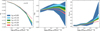 |
Fig. 2 Halo bias parameters as a function of mass in the Planck simulation. Different colors indicate the damping scale (kd), measured in [hMpc−1], used to smooth the Lagrangian fields employed in the measurement of the bias parameters, and the colored regions indicate the 1σ interval around the mean value. Values presented here were measured for halos at z = 0, and the measurements at higher redshifts are even less dependent on kd, so any conclusion on the convergence of the estimators obtained here are also valid at other times. |
4 Results
In this section we present the results of applying our shape bias estimators to halos in the simulations described in the previous section. Before presenting the results, we emphasize that we can estimate cK and cK⊗K for each individual object. This gives us great flexibility since once this set of biases is measured, we can average them over any quantity of interest, provided it is a small-scale property of the halos. To avoid confusion, we state clearly in the figure caption the quantity used for binning since it might not be the one being displayed.
4.1 Validation of estimators
As described in Sect. 2, our bias estimators require smoothing the Lagrangian density field on an arbitrary scale kd in Fourier space. An important validation is to make sure that our estimates are, in fact, independent of kd if we make it sufficiently small (since bias parameters are formally scale-independent quantities). Figure 2 shows the measurements of cK, cδK and cK⊗K averaged in bins of halo mass for increasing values of kd. These measurements are displayed in the figure as shaded bands marking the 1σ region around the mean value of the biases. One can see that the measurements using kd = 0.05 [hMpc−1] and kd = 0.1 [hMpc−1] are compatible within 1σ over all masses, with the exception of the largest mass bin for cK⊗K, for which these estimators are compatible within 1.5σ. Based on these checks, we adopted kd = 0.1 [hMpc−1] as the smallest scale at which our estimators are scale-independent and used it to estimate all bias parameters that appear in the following.
To validate our method, we compared the results to previous measurements in the literature (Stücker et al. 2021; Akitsu et al. 2021, 2023). In Fig. 3 we compare cδK and cK⊗K versus cK for halos in different mass bins. Different colored lines represent different halo-shape definitions. Comparing the results for our standard definition, IFoF, to the measurements of Akitsu et al. (2023) shows similar trends but a significant quantitative disagreement. However, the shapes of halos are expected to be very dependent on the halo definition used. Shape definitions based on spherical overdensity, such as ℐ200,c, ℐ500,c, and ℐ200,b, produce more isotropic halos due to the fact that the particles belonging to the halo are preselected to be in a spherical region. On the other hand, the FoF shape definition allows the halo out-skirts to have varying shapes, which can heavily influence the measurement of ℐFoF.
If we compare the measurements of Akitsu et al. (2023) to our results for spherical boundary definitions – in particular the reduced inertia tensor ![Mathematical equation: $\[\tilde{\mathcal{I}}_{200, \mathrm{b}}\]$](/articles/aa/full_html/2025/07/aa53212-24/aa53212-24-eq58.png) – we find a good agreement. Since these authors use the Amiga’s halo finder (Knollmann & Knebe 2009), a spherical-overdensity based halo-finder, to define their halos and compute their bias parameters with the reduced shape tensor, this is the comparison that makes the most sense. The agreement is particularly good for
– we find a good agreement. Since these authors use the Amiga’s halo finder (Knollmann & Knebe 2009), a spherical-overdensity based halo-finder, to define their halos and compute their bias parameters with the reduced shape tensor, this is the comparison that makes the most sense. The agreement is particularly good for ![Mathematical equation: $\[\tilde{\mathcal{I}}_{200, \mathrm{b}}\]$](/articles/aa/full_html/2025/07/aa53212-24/aa53212-24-eq59.png) , which is unsurprising since those authors employ the same definition for the halo boundary. Therefore, we consider our measurements to be consistent with those reported by Akitsu et al. (2023), but we note that care must be taken when comparing different halo definitions – much more so than, for example, when comparing halo density bias parameters. As the tidal alignment of halos is not directly observationally relevant, the preferential definition is not clear, and we stuck to the FoF boundary for simplicity. However, we note that, for example for measuring the alignment of galaxies in simulations, it is advisable to use definitions that match observational criteria (Tenneti et al. 2015b).
, which is unsurprising since those authors employ the same definition for the halo boundary. Therefore, we consider our measurements to be consistent with those reported by Akitsu et al. (2023), but we note that care must be taken when comparing different halo definitions – much more so than, for example, when comparing halo density bias parameters. As the tidal alignment of halos is not directly observationally relevant, the preferential definition is not clear, and we stuck to the FoF boundary for simplicity. However, we note that, for example for measuring the alignment of galaxies in simulations, it is advisable to use definitions that match observational criteria (Tenneti et al. 2015b).
4.2 Universal relations
As mentioned at the beginning of this section, our method has the advantage of being very flexible and allowing the measurement of shape bias parameters averaged over any quantity of choice. Figure 4 shows the shape bias parameters measured from the halos in the Planck and Narya-HD simulations, averaged directly in peak height ν = δc/σ(M, z), where σ(M, z) is defined as
![Mathematical equation: $\[\sigma(M, z)^2=\int \frac{d^3 \mathbf{k}}{(2 \pi)^3} P(k, z) W^2(k R),\]$](/articles/aa/full_html/2025/07/aa53212-24/aa53212-24-eq60.png) (49)
(49)
where ![Mathematical equation: $\[R=\left(\frac{3 M}{4 \pi \bar{\rho}}\right)^{1 / 3}, ~\bar{\rho}\]$](/articles/aa/full_html/2025/07/aa53212-24/aa53212-24-eq62.png) is the mean density of the universe, and W is a top-hat profile in Fourier space:
is the mean density of the universe, and W is a top-hat profile in Fourier space:
![Mathematical equation: $\[W(k R)=\frac{1}{(k R)^2}\left(\frac{3 ~\sin~ (k R)}{k R}-~\cos (k R)\right).\]$](/articles/aa/full_html/2025/07/aa53212-24/aa53212-24-eq63.png) (50)
(50)
This quantity is commonly used in excursion-set theory to measure how likely it is that the density in a region of radius R has crossed δc, the threshold for collapse. The relations in terms of ν are universal, that is, they do not depend on redshift or cosmology. Furthermore, we notice that the functional forms relating the shape biases to ν can be described by simple linear or quadratic functions, which get damped at very low ν, much simpler than those relating the shape biases to b1. Fits for the relation of the IA biases with ν are provided in Table 3. For comparison, we also show these relations with b1 in Fig. 5 with fits as listed in Table 4.
The fact that cK depends strongly on ν is very revealing about the nature of alignments. Let us consider the hypothesis that halos get their alignments through the dynamical effect of the tidal field after formation. The tidal field may slightly distort the virialized halos – shifting them to an anisotropic equilibrium configuration. We refer to this as the “post-formation-response” scenario. Such a mechanism has been considered in several studies to explain the IA of galaxies (e.g., Tugendhat & Schäfer 2018; Zjupa et al. 2020; Ghosh et al. 2024), but it could also be a plausible effect for halos.
If post-formation-response is the primary alignment mechanism of halos, then the degree of alignment should depend primarily on the anisotropy of the gravitational field in the vicinity of the halo. For a spherical halo with mass profile M(r) plus a traceless large-scale tide K, the gravitational acceleration is given by
![Mathematical equation: $\[\boldsymbol{a}(\boldsymbol{r})=4 \pi G \rho_m \mathbf{K} \boldsymbol{r}-\frac{G M(r)}{r^3} \boldsymbol{r},\]$](/articles/aa/full_html/2025/07/aa53212-24/aa53212-24-eq64.png)
where the factor 4πGρm is needed to correct for the dimensionless form of K. If we consider an Navarro–Frenk–White halo at the virial radius r200c, we can define the effective tidal tensor at the scale of the halo:
![Mathematical equation: $\[\begin{aligned}T_{200 \mathrm{c}} & =4 \pi G \rho_{\mathrm{m}} \mathbf{K}-\frac{G M_{200 \mathrm{c}}}{r_{200 \mathrm{c}}^3} \mathbf{J}_2 \\& =4 \pi G \rho_{\mathrm{m}}\left(\mathbf{K}-\frac{200}{3} \mathbf{J}_2\right),\end{aligned}\]$](/articles/aa/full_html/2025/07/aa53212-24/aa53212-24-eq65.png) (51)
(51)
where J2 is the unit matrix. The isotropic component is sourced purely by the halo, and the anisotropic component purely by the large-scale tide. Therefore, the relative anisotropy in the gravitational field of an already formed halo is on the order 3K1/200 (where K1 is the largest eigenvalue of K). The anisotropy in the triggered density response should be proportional to this and should probably also not be larger in amplitude. Therefore, we expect a post-formation-response that is mass-independent and of order |cK| ≲ 10−2. This simple expectation clearly disagrees with the measured cK relations, which exhibit a strong mass (or ν) dependence and a much larger degree of alignment up to |cK| ≲ 0.5. We conclude, therefore, that post-formation-response is not the dominant mechanism for the alignment of halos (see Camelio & Lombardi 2015, for a similar consideration for the case of galaxies). The anisotropy must already be encoded during the formation and accretion processes.
We speculated about three possible scenarios that could explain how the ν dependence of cK is encoded during formation. (1) The tidal field only significantly introduces anisotropy up to the formation of a halo and becomes irrelevant at later times. In this scenario, halos that form earlier have a lesser response because they have formed in a weaker tidal field. Combined with the fact that a smaller ν leads to an earlier formation, this could qualitatively explain the observed trend. However, it is unclear whether this could match the measurements quantitatively and whether it is consistent with the observed universality. (2) Halos at low ν (and therefore large variance) are born in significantly larger tidal fields than halos at high ν. The relative changes in the tidal tensor at the halo scale due to an imposed large-scale tidal field are, therefore, much smaller for small halos. (3) Halo shapes are not responding as a continuous deformation to the large-scale tidal field but are rather governed by discrete events – for example through the formation of larger-scale pancakes and filaments. The response of small halos may then be small because they are almost all embedded in larger-scale filaments, so it is unlikely that an increase in the tidal field triggers an additional filament formation. Such a process could be described through an excursion set formalism, which naturally leads to universality.
While so far a clear understanding of the formation of shapes is elusive, we note that there may be some hope to gain further insights: (a) The simple universal form of the response motivates the notion that a simple description exists – similar to the way that excursion sets offer a quite reasonable model for the density biases of halos. (b) All the abovementioned scenarios could be turned into simple models with quantitative predictions that can be easily tested. (c) The response of halos could be investigated in warm dark matter simulations. The smallest warm dark matter halos have a clear and well-defined formation time and size (Diemand et al. 2005; Ishiyama et al. 2010; Angulo et al. 2017; Ogiya & Hahn 2018; Ondaro-Mallea et al. 2024). It would be insightful to explore how such objects respond to tides before and after formation. (d) Some of the points above can be studied in anisotropic SU simulations. For example, for (2) to be correct, the differential response |∂/∂T0⟨I|T0⟩g| at large values of the tidal field should be notably smaller than the response at T0 = 0.
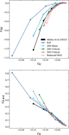 |
Fig. 3 Comparison of shape-bias measurements performed in the Planck simulation with a range of different halo definitions to the measurements reported in Akitsu et al. (2023). There is a large variability in the relations found, of which |
![Mathematical equation: $\[\tilde{\mathcal{I}}_{200, \mathrm{b}}\]$](/articles/aa/full_html/2025/07/aa53212-24/aa53212-24-eq61.png)
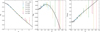 |
Fig. 4 Measurements of shape bias parameters in the Planck simulation as a function of peak-significance ν = δc/σ(M, z). All measurements, regardless of redshift, seem to follow a common trend with ν. Solid black lines show the fits performed to approximate these common relations. These fitting functions are exceptionally simple – linear for cK and cK⊗K and quadratic for cδK – and provide good descriptions of the measured relations. |
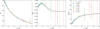 |
Fig. 5 Shape biases in the Planck simulation averaged over bins in ν = δc/σ(M, z), the peak-significance, as a function of linear density bias (b1), also averaged over bins of ν. Different colors represent the redshifts indicated in the legend. Each panel shows the orthogonal distance of the measurements to the fit, in units of the measurement error. The postulated functions provide a good description of the relations between the shape biases and b1. |
Fitting functions.
Fitting functions.
4.3 Assembly bias
In addition to the dependence of halo IA bias on ν, it is interesting to explore whether splitting the same ν populations by some secondary property would result in significantly distinct signals. We explored this possibility by splitting our samples according to their spin, which is defined as (Bullock et al. 2001)
![Mathematical equation: $\[\lambda=\frac{|\mathbf{L}|}{\sqrt{2} v_{200, c} r_{200, c}},\]$](/articles/aa/full_html/2025/07/aa53212-24/aa53212-24-eq67.png) (52)
(52)
where
![Mathematical equation: $\[\mathbf{L}=\langle\mathbf{r} \times \mathbf{v}\rangle_{\text {particles}},\]$](/articles/aa/full_html/2025/07/aa53212-24/aa53212-24-eq68.png) (53)
(53)
is the specific angular momentum vector of the object. We then split the population at each bin of ν into four quartiles of the spin distribution such that Q1 contains the halos with the 25% smallest spins and Q4 the 25% largest. Figure 6 shows the ratios between the biases of these subpopulations and the bias of the full sample. We can see that at low masses, the amplitude of ![Mathematical equation: $\[c_{K}^{Q}\]$](/articles/aa/full_html/2025/07/aa53212-24/aa53212-24-eq69.png) is anticorrelated with spin: lower-spin halos have a higher bias and higher-spin halos have a lower bias. This trend is inverted around ν ≈ 1.75, and beyond that the amplitude of cK is larger for high-spin halos and smaller for low-spin ones. As far as we are aware, this is the first time that a secondary dependence of cK on halo spin is observed.
is anticorrelated with spin: lower-spin halos have a higher bias and higher-spin halos have a lower bias. This trend is inverted around ν ≈ 1.75, and beyond that the amplitude of cK is larger for high-spin halos and smaller for low-spin ones. As far as we are aware, this is the first time that a secondary dependence of cK on halo spin is observed.
It is well known that the linear density bias of halos b1 has a secondary dependence on spin (Gao & White 2007), and hence it is interesting to probe whether the dependence of cK with spin is simply a consequence of the dependence of b1 with spin. With that purpose, in Fig. 7, we show cK and b1 averaged over ν bins and split into subpopulations by spin, as described earlier. One can clearly see the assembly bias in b1 – measurements that have the same ν are connected by dashed lines, and they have different values of b1 depending on the spin-quartile they belong to. Nevertheless, one can also identify an independent cK assembly bias signal since cK does not vary along the b1 − cK relation at fixed ν with varying spin.
5 Conclusions
In this article we have presented a new methodology for computing shape biases in cosmological simulations from correlations in the distribution of the initial tidal tensor and the final shapes of objects.
Our method is conceptually similar to the anisotropic SU approach (Stücker et al. 2021; Akitsu et al. 2021) and provides a robust measurement of the shape bias parameters that is independent of the number of considered parameters – in notable contrast to methods that need to fit a model to power spectra or even field-level measurements (Zennaro et al. 2022; Schmittfull et al. 2019). We have shown that for sufficiently large damping scales, kd ≤ 0.1h/Mpc, our method is independent of the damping scale and matches the results from SU simulations. However, the new method allows us to perform these measurements at a much reduced computational cost for an arbitrary set of parameters from a single simulation – making it viable for application in modern hydrodynamical simulations.
The application of these estimators to simulated halos has allowed us to quantify the dependence of the bias parameters cK, cδK, and cK⊗K on the peak height (ν) and linear density bias (b1), and to provide fitting functions that accurately describe these relations. The strong mass dependence of the alignment response shows that the anisotropy must already be encoded during the formation and accretion history of objects. The post-formation-response – as it is considered in some models of galaxy alignment (e.g., Tugendhat & Schäfer 2018; Zjupa et al. 2020; Ghosh et al. 2024) – is too weak and too mass-independent to explain the linear large-scale alignment of halos.
Further, we have presented the first detection of the dependence of the tidal alignment response (cK) on the spin of halos at a fixed peak height. This secondary dependence is rather complicated, leading to a greater response for higher spins at high masses but a lesser response for higher spins at lower masses. Understanding this relation may pose a significant challenge for analytical approaches to modeling alignments and tidal torquing (e.g., White 1984).
The response of halo shapes to the large-scale tidal field provides important qualitative insights into collisionless systems and the ingredients that are necessary to model IAs. However, quantitatively, it is far more relevant to understand the alignment of galaxies – in particular, to correctly interpret weak-lensing observations. While we have validated our method in the case of halos in this article, it can easily be applied to simulated galaxies as well – an avenue that we will explore in future studies.
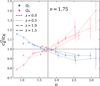 |
Fig. 6 Measurements of linear shape bias in the Planck simulation, averaged over bins of ν, for halos selected in the lowest and highest quartiles in the distribution of spins. A clear assembly bias signal is detected: for low values of ν, objects with low (high) spin have an above (below) average cK value; this behavior is inverted around ν* = 1.75, as marked by the vertical black line. |
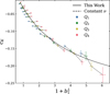 |
Fig. 7 Linear shape bias as a function of linear density bias in the Planck simulation. Different colors represent the quartiles in the distribution of halo spins. One can clearly see a difference in the values of cK even at fixed b1, which indicates a nontrivial assembly-bias signal. |
Acknowledgements
The authors thank Kazuyuki Akitsu for providing his measurements at our request. The authors acknowledge support from the Spanish Ministry of Science under grant number PID2021-128338NB-I00 and from the European Research Executive Agency HORIZON-MSCA-2021-SE-01 Research and Innovation programme under the Marie Sklodowska-Curie grant agreement number 101086388 (LACEGAL).
Appendix A Notation
In this section we define some conventions in notation to be used throughout this work. This is particularly relevant because we define some convenient ways to define operations between tensors that appear frequently in this paper. Table A.1 resumes the definitions for most of the symbols employed throughout this article. Table A.2 resumes several of the most important notation for tensor operations used throughout this manuscript.
General notation employed throughout the article.
Notation for tensor operations.
Appendix B Isotropic tensors
In this appendix we condense the results of Stücker et al. (2025) by determining an orthogonal basis for all isotropic tensors of rank n that respect the following symmetry: let Mi0i1...i2n,i2n+1... be an isotropic tensor. Then we required M to be symmetric using the interchange i2n ↔ i2n+1. For tensors of rank 1, there is only one such tensor, the Kronecker delta symbol,
![Mathematical equation: $\[\mathbf{J}_2=\delta_{i j}^K.\]$](/articles/aa/full_html/2025/07/aa53212-24/aa53212-24-eq78.png) (B.1)
(B.1)
For rank-4 tensors, there are two such tensors,
![Mathematical equation: $\[\mathbf{J}_{22}=\delta_{i j}^K \delta_{k l}^K\]$](/articles/aa/full_html/2025/07/aa53212-24/aa53212-24-eq79.png) (B.2)
(B.2)
![Mathematical equation: $\[\mathbf{J}_{2=2}=S_{22}\left(\delta_{i j}^K \delta_{k l}^K\right)-\frac{1}{3} \mathbf{J}_{22};\]$](/articles/aa/full_html/2025/07/aa53212-24/aa53212-24-eq80.png) (B.3) (B.4)
(B.3) (B.4)
the subscripts indicate properties of these tensors, namely that by contracting J22 with two rank-2 tensors A and B, one obtains the product of their traces – so there is no mixing of their components. By performing the same calculation with J2=2, on the other hand, one obtains the trace of their matrix product. In fact, each “-” symbol in the subscripts represents one index contraction between tensors A and B. Finally, for rank 6 there are five different tensors
![Mathematical equation: $\[\mathbf{J}_{222}=\delta_{i j}^K \delta_{k l}^K \delta_{m n}^K\]$](/articles/aa/full_html/2025/07/aa53212-24/aa53212-24-eq82.png) (B.5)
(B.5)
![Mathematical equation: $\[\mathbf{J}_{22=2}=S_{222}\left(\delta_{i j}^K \delta_{k n}^K \delta_{m l}^K\right)-\frac{1}{3} \mathbf{J}_{222}\]$](/articles/aa/full_html/2025/07/aa53212-24/aa53212-24-eq83.png) (B.6)
(B.6)
![Mathematical equation: $\[\mathbf{J}_{2=22}=S_{222}\left(\delta_{i l}^K \delta_{k j}^K \delta_{m n}^K\right)-\frac{1}{3} \mathbf{J}_{222}\]$](/articles/aa/full_html/2025/07/aa53212-24/aa53212-24-eq84.png) (B.7)
(B.7)
![Mathematical equation: $\[\mathbf{J}_{222}=S_{222}\left(\delta_{i n}^K \delta_{k l}^K \delta_{m j}^K\right)-\frac{1}{3} \mathbf{J}_{222}\]$](/articles/aa/full_html/2025/07/aa53212-24/aa53212-24-eq85.png) (B.8)
(B.8)
![Mathematical equation: $\[\mathbf{J}_{2-2-2-}=S_{222}\left(\delta_{i k}^K \delta_{l m}^K \delta_{n j}^K\right)-\frac{1}{9} \mathbf{J}_{222}-\frac{1}{3}\left(\mathbf{J}_{22=2}+\mathbf{J}_{2=22}+\mathbf{J}_{222=}\right).\]$](/articles/aa/full_html/2025/07/aa53212-24/aa53212-24-eq86.png) (B.9)
(B.9)
Appendix C Shape convergence
In this appendix we present measurements of the shape-bias parameters obtained from two simulations, both run with Narya cosmology but at different resolutions. This test allows us to define a convergence criterion, which is used throughout the entire article. As can be seen from Fig. C.1, these bias parameters are in agreement with each other for Mh > 1012M⊙h−1. This mass corresponds to halos with roughly 270 particles in the low-resolution Narya simulation, so we defined our convergence criterion to be that halos must have more than 300 particles.
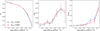 |
Fig. C.1 Comparison of measurements of shape-biases cK, cδK, and cK⊗K in two versions of the Narya simulation, with increasing resolution. For these measurements, shapes were computed using the FoF halo definition. One can see that the results generally match within the error bars, except for measurements of cK below M200,b = 1012M⊙h−1. The damping scale employed in measuring these bias parameters is kd = 0.1hMpc−1 |
Appendix D Comparison to the literature
Similar measurements to the ones reported in this article were performed by Akitsu et al. (2023), but for the Eulerian bias parameters. Nevertheless, in that work, they present expressions for translating the bias parameters from Eulerian to Lagrangian space. Therefore, when comparing our results to theirs, we always converted our measurements using Eq. (2.15) of Akitsu et al. (2023).
References
- Akitsu, K., Li, Y., & Okumura, T. 2021, J. Cosmology Astropart. Phys., 2021, 041 [Google Scholar]
- Akitsu, K., Li, Y., & Okumura, T. 2023, J. Cosmology Astropart. Phys., 2023, 068 [CrossRef] [Google Scholar]
- Angulo, R. E., & Pontzen, A. 2016, MNRAS, 462, L1 [NASA ADS] [CrossRef] [Google Scholar]
- Angulo, R. E., Baugh, C. M., & Lacey, C. G. 2008, MNRAS, 387, 921 [NASA ADS] [CrossRef] [Google Scholar]
- Angulo, R. E., Hahn, O., Ludlow, A. D., & Bonoli, S. 2017, MNRAS, 471, 4687 [Google Scholar]
- Angulo, R. E., Zennaro, M., Contreras, S., et al. 2021, MNRAS, 507, 5869 [NASA ADS] [CrossRef] [Google Scholar]
- Aricò, G., Angulo, R. E., Zennaro, M., et al. 2023, A&A, 678, A109 [NASA ADS] [CrossRef] [EDP Sciences] [Google Scholar]
- Assassi, V., Baumann, D., Green, D., & Zaldarriaga, M. 2014, J. Cosmology Astropart. Phys., 2014, 056 [CrossRef] [Google Scholar]
- Bakx, T., Kurita, T., Chisari, N. E., Vlah, Z., & Schmidt, F. 2023, J. Cosmology Astropart. Phys., 2023, 005 [Google Scholar]
- Bardeen, J. M., Bond, J. R., Kaiser, N., & Szalay, A. S. 1986, ApJ, 304, 15 [Google Scholar]
- Blazek, J., Vlah, Z., & Seljak, U. 2015, J. Cosmology Astropart. Phys., 2015, 015 [CrossRef] [Google Scholar]
- Bond, J. R., Cole, S., Efstathiou, G., & Kaiser, N. 1991, ApJ, 379, 440 [NASA ADS] [CrossRef] [Google Scholar]
- Bullock, J. S., Kolatt, T. S., Sigad, Y., et al. 2001, MNRAS, 321, 559 [Google Scholar]
- Camelio, G., & Lombardi, M. 2015, A&A, 575, A113 [NASA ADS] [CrossRef] [EDP Sciences] [Google Scholar]
- Catelan, P., Kamionkowski, M., & Blandford, R. D. 2001, MNRAS, 320, L7 [NASA ADS] [CrossRef] [Google Scholar]
- Chen, S.-F., & Kokron, N. 2024, J. Cosmology Astropart. Phys., 2024, 027 [CrossRef] [Google Scholar]
- Chisari, N., Codis, S., Laigle, C., et al. 2015, MNRAS, 454, 2736 [NASA ADS] [CrossRef] [Google Scholar]
- Contreras, S., Angulo, R. E., Chaves-Montero, J., et al. 2024, A&A, 690, A311 [NASA ADS] [CrossRef] [EDP Sciences] [Google Scholar]
- Croton, D. J., Gao, L., & White, S. D. M. 2007, MNRAS, 374, 1303 [Google Scholar]
- Dalal, N., White, M., Bond, J. R., & Shirokov, A. 2008, ApJ, 687, 12 [NASA ADS] [CrossRef] [Google Scholar]
- Delgado, A. M., Hadzhiyska, B., Bose, S., et al. 2023, MNRAS, 523, 5899 [CrossRef] [Google Scholar]
- Desjacques, V., Jeong, D., & Schmidt, F. 2018, Phys. Rep., 733, 1 [Google Scholar]
- Diemand, J., Moore, B., & Stadel, J. 2005, Nature, 433, 389 [Google Scholar]
- Gao, L., & White, S. D. M. 2007, MNRAS, 377, L5 [NASA ADS] [CrossRef] [Google Scholar]
- Gao, L., Springel, V., & White, S. D. M. 2005, MNRAS, 363, L66 [NASA ADS] [CrossRef] [Google Scholar]
- Ghosh, B., Nussbaumer, K., Giesel, E. S., & Schäfer, B. M. 2024, Open J. Astrophys., 7, 41 [Google Scholar]
- Gnedin, N. Y., Kravtsov, A. V., & Rudd, D. H. 2011, ApJS, 194, 46 [Google Scholar]
- Hilbert, S., Xu, D., Schneider, P., et al. 2017, MNRAS, 468, 790 [Google Scholar]
- Hirata, C. M., & Seljak, U. c. v. 2004, Phys. Rev. D, 70, 063526 [NASA ADS] [CrossRef] [Google Scholar]
- Ishiyama, T., Makino, J., & Ebisuzaki, T. 2010, ApJ, 723, L195 [Google Scholar]
- Ivanov, M. M., Cuesta-Lazaro, C., Mishra-Sharma, S., Obuljen, A., & Toomey, M. W. 2024, arXiv e-prints [arXiv:2402.13310] [Google Scholar]
- Ivanov, M. M., Obuljen, A., Cuesta-Lazaro, C., & Toomey, M. W. 2025, Phys. Rev. D, 111, 063548 [Google Scholar]
- Joachimi, B., Cacciato, M., Kitching, T. D., et al. 2015, Space Sci. Rev., 193, 1 [Google Scholar]
- Kiessling, A., Cacciato, M., Joachimi, B., et al. 2015, Space Sci. Rev., 193, 67 [Google Scholar]
- Kirk, D., Brown, M. L., Hoekstra, H., et al. 2015, Space Sci. Rev., 193, 139 [Google Scholar]
- Knollmann, S. R., & Knebe, A. 2009, ApJS, 182, 608 [Google Scholar]
- Lacey, C., & Cole, S. 1993, MNRAS, 262, 627 [NASA ADS] [CrossRef] [Google Scholar]
- Maion, F., Angulo, R. E., Bakx, T., et al. 2024, MNRAS, 531, 2684 [NASA ADS] [CrossRef] [Google Scholar]
- Mandelbaum, R. 2018, ARA&A, 56, 393 [Google Scholar]
- Ogiya, G., & Hahn, O. 2018, MNRAS, 473, 4339 [Google Scholar]
- Ondaro-Mallea, L., Angulo, R. E., Stücker, J., Hahn, O., & White, S. D. M. 2024, MNRAS, 527, 10802 [Google Scholar]
- Planck Collaboration VI. 2020, A&A, 641, A6 [NASA ADS] [CrossRef] [EDP Sciences] [Google Scholar]
- Preston, C., Amon, A., & Efstathiou, G. 2024, MNRAS, 533, 621 [NASA ADS] [CrossRef] [Google Scholar]
- Rubira, H., & Schmidt, F. 2024, J. Cosmology Astropart. Phys., 2024, 031 [Google Scholar]
- Schmidt, A. S., White, S. D. M., Schmidt, F., & Stücker, J. 2018, MNRAS, 479, 162 [NASA ADS] [CrossRef] [Google Scholar]
- Schmittfull, M., Baldauf, T., & Seljak, U. 2015, Phys. Rev. D, 91, 043530 [Google Scholar]
- Schmittfull, M., Simonović, M., Assassi, V., & Zaldarriaga, M. 2019, Phys. Rev. D, 100, 043514 [NASA ADS] [CrossRef] [Google Scholar]
- Secco, L., Samuroff, S., Krause, E., et al. 2022, Phys. Rev. D, 105 [Google Scholar]
- Shiferaw, M., Kokron, N., & Wechsler, R. H. 2024, arXiv e-prints [arXiv:2412.06886] [Google Scholar]
- Springel, V. 2005, MNRAS, 364, 1105 [Google Scholar]
- Stücker, J., Schmidt, A. S., White, S. D. M., Schmidt, F., & Hahn, O. 2021, MNRAS, 503, 1473 [CrossRef] [Google Scholar]
- Stücker, J., Pellejero-Ibáñez, M., Angulo, R. E., Maion, F., & Voivodic, R. 2025, A&A, 699, A197 [NASA ADS] [CrossRef] [EDP Sciences] [Google Scholar]
- Tenneti, A., Mandelbaum, R., & Di Matteo, T. 2016, MNRAS, 462, 2668 [Google Scholar]
- Tenneti, A., Kitching, T. D., Joachimi, B., & Di Matteo, T. 2020, MNRAS, 501, 5859 [Google Scholar]
- Tenneti, A., Mandelbaum, R., Di Matteo, T., Feng, Y., & Khandai, N. 2014, MNRAS, 441, 470 [Google Scholar]
- Tenneti, A., Mandelbaum, R., Di Matteo, T., Kiessling, A., & Khandai, N. 2015a, MNRAS, 453, 469 [Google Scholar]
- Tenneti, A., Singh, S., Mandelbaum, R., et al. 2015b, MNRAS, 448, 3522 [Google Scholar]
- Troxel, M., & Ishak, M. 2015, Phys. Rep., 558, 1 [NASA ADS] [CrossRef] [Google Scholar]
- Tugendhat, T. M., & Schäfer, B. M. 2018, MNRAS, 476, 3460 [Google Scholar]
- Velliscig, M., Cacciato, M., Schaye, J., et al. 2015, MNRAS, 454, 3328 [CrossRef] [Google Scholar]
- Vlah, Z., Chisari, N. E., & Schmidt, F. 2020, MNRAS, 2020, 025 [Google Scholar]
- Vlah, Z., Chisari, N. E., & Schmidt, F. 2021, J. Cosmology Astropart. Phys., 2021, 061 [Google Scholar]
- Wagner, C., Schmidt, F., Chiang, C.-T., & Komatsu, E. 2014, MNRAS, 448, L11 [Google Scholar]
- Wechsler, R. H., Zentner, A. R., Bullock, J. S., Kravtsov, A. V., & Allgood, B. 2006, ApJ, 652, 71 [NASA ADS] [CrossRef] [Google Scholar]
- White, S. D. M. 1984, ApJ, 286, 38 [NASA ADS] [CrossRef] [Google Scholar]
- Zehavi, I., Contreras, S., Padilla, N., et al. 2018, ApJ, 853, 84 [NASA ADS] [CrossRef] [Google Scholar]
- Zennaro, M., Angulo, R. E., Contreras, S., Pellejero-Ibáñez, M., & Maion, F. 2022, MNRAS, 514, 5443 [NASA ADS] [CrossRef] [Google Scholar]
- Zhang, H., Bonici, M., D’Amico, G., Paradiso, S., & Percival, W. J. 2024, arxiv e-prints [arXiv:2409.12937] [Google Scholar]
- Zheng, Z., Berlind, A. A., Weinberg, D. H., et al. 2005, ApJ, 633, 791 [NASA ADS] [CrossRef] [Google Scholar]
- Zjupa, J., Schäfer, B. M., & Hahn, O. 2020, arXiv e-prints [arXiv:2010.07951] [Google Scholar]
All Tables
All Figures
|
Fig. 1 Illustration of halo shapes in a simulation slice and their relation to the underlying density and tidal fields. Left: density field linearly extrapolated to z = 0 (background), with a large set of small arrows superimposed. The sizes of these small arrows are scaled to the local projected tidal field’s largest eigenvalue, and their direction is that of the corresponding eigenvector. Middle: halos (colored ellipses) centered at their Lagrangian positions. Their shapes are those of the projected shape tensor estimated for the FoF group; their color corresponds to the value of their three-dimensional shape-alignment bias. Right: same as the middle panel except now the halos are at their final Eulerian positions. |
| In the text | |
|
Fig. 2 Halo bias parameters as a function of mass in the Planck simulation. Different colors indicate the damping scale (kd), measured in [hMpc−1], used to smooth the Lagrangian fields employed in the measurement of the bias parameters, and the colored regions indicate the 1σ interval around the mean value. Values presented here were measured for halos at z = 0, and the measurements at higher redshifts are even less dependent on kd, so any conclusion on the convergence of the estimators obtained here are also valid at other times. |
| In the text | |
|
Fig. 3 Comparison of shape-bias measurements performed in the Planck simulation with a range of different halo definitions to the measurements reported in Akitsu et al. (2023). There is a large variability in the relations found, of which |
| In the text | |
|
Fig. 4 Measurements of shape bias parameters in the Planck simulation as a function of peak-significance ν = δc/σ(M, z). All measurements, regardless of redshift, seem to follow a common trend with ν. Solid black lines show the fits performed to approximate these common relations. These fitting functions are exceptionally simple – linear for cK and cK⊗K and quadratic for cδK – and provide good descriptions of the measured relations. |
| In the text | |
|
Fig. 5 Shape biases in the Planck simulation averaged over bins in ν = δc/σ(M, z), the peak-significance, as a function of linear density bias (b1), also averaged over bins of ν. Different colors represent the redshifts indicated in the legend. Each panel shows the orthogonal distance of the measurements to the fit, in units of the measurement error. The postulated functions provide a good description of the relations between the shape biases and b1. |
| In the text | |
|
Fig. 6 Measurements of linear shape bias in the Planck simulation, averaged over bins of ν, for halos selected in the lowest and highest quartiles in the distribution of spins. A clear assembly bias signal is detected: for low values of ν, objects with low (high) spin have an above (below) average cK value; this behavior is inverted around ν* = 1.75, as marked by the vertical black line. |
| In the text | |
|
Fig. 7 Linear shape bias as a function of linear density bias in the Planck simulation. Different colors represent the quartiles in the distribution of halo spins. One can clearly see a difference in the values of cK even at fixed b1, which indicates a nontrivial assembly-bias signal. |
| In the text | |
|
Fig. C.1 Comparison of measurements of shape-biases cK, cδK, and cK⊗K in two versions of the Narya simulation, with increasing resolution. For these measurements, shapes were computed using the FoF halo definition. One can see that the results generally match within the error bars, except for measurements of cK below M200,b = 1012M⊙h−1. The damping scale employed in measuring these bias parameters is kd = 0.1hMpc−1 |
| In the text | |
Current usage metrics show cumulative count of Article Views (full-text article views including HTML views, PDF and ePub downloads, according to the available data) and Abstracts Views on Vision4Press platform.
Data correspond to usage on the plateform after 2015. The current usage metrics is available 48-96 hours after online publication and is updated daily on week days.
Initial download of the metrics may take a while.