© The Authors 2025

1. Introduction

Galaxy clusters (clusters from now on) are the largest gravitationally bound structures in the universe, containing hundreds (sometimes thousands) of galaxies along with vast amounts of hot intracluster gas and dark matter. Clusters form in regions with a much higher than average density in the early universe, making them crucial for understanding the large-scale cosmic architecture.

A significant portion of a cluster's mass comes in the form of dark matter. Studying the distribution and effects of dark matter in galaxy clusters helps us learn about its properties. As dark matter does not emit, absorb, or scatter light in any measurable amount, we can only quantify its distribution via its gravitational influence. One such influence is gravitational lensing, which occurs when a massive object bends the light from a more distant object behind it. The mass of the cluster acts like a lens, distorting, magnifying, and sometimes creating multiple images of the background object. By analyzing the positions and shapes of these arcs and images, we can infer the distribution of mass that is causing the lensing.

Traditional approaches to modeling cluster mass typically involve identifying the positions of multiple images of lensed sources, calculating where these images map onto the source plane using the current lens model, and ensuring that the multiple images of the same source converge to the same point on this plane (Meneghetti et al. 2017). This process takes the full telescope image of the cluster and reduces it to a summary data vector, which is much faster to fit. In a typical cluster lens, tens to hundreds of multiply imaged sources may be present, providing useful constraints for the lens model and making modeling feasible, especially when additional observational information is used from stellar kinematics (Monna et al. 2017; Bergamini et al. 2019). Nevertheless, this data reduction results in a significant loss of information. These steps are deemed necessary because the full image of a cluster lens is typically too large to analyze at the pixel level, often containing millions of pixels, which makes the ray tracing calculations computationally costly. Additionally, global cluster lens models are often not worth fitting the pixel-level data as they can have root mean square values rarely less than 0.1″ and sometimes as high as 0.5″ for the differences between the model predicted and observed positions (Caminha et al. 2016, 2019), failing to reach sub-pixel precision. To address this challenge, our work focuses on multiple images of a single source that is stretched into a lensed arc, with the goal of building a lens model that can precisely fit the angular deflections near the arc. The critical curves of cluster lenses provide the highest magnification regions in the sky. This powerful magnification boosts the apparent luminosity of distant objects that would otherwise be difficult to detect. There are several ongoing science cases, mainly involving the study of these highly magnified objects, which would benefit from precise modeling of extended arcs in clusters: caustic crossings of individual stars (Kelly et al. 2018; Chen et al. 2019; Kaurov et al. 2019; Welch et al. 2022a, b; Furtak et al. 2023; Diego et al. 2023a, b; Meena et al. 2023), gravitationally lensed supernovae (Kelly et al. 2015; Rodney et al. 2021; Chen et al. 2022; Frye et al. 2024; Pierel et al. 2024), and star clusters (Adamo et al. 2024). Having more precise lens models near the critical curve is crucial in making robust inferences on the source properties in all of these cases, leading to a better understanding of the nature of these highly magnified objects.

A new approach to modeling cluster lenses at pixel-level was previously employed by Şengül et al. (2023), where the multiple images of a source galaxy lensed by a cluster are analyzed by a local lens model called curved arc basis (CAB) first proposed by Birrer (2021). The main limitation of CAB is that as an approximation, it fails if the magnified arc covers a large extended region or when the angular deflections change significantly over a short distance. Therefore, it is suitable for modeling sets of multiple images of a source that are either far from the critical curve or small in extent. For this reason, the magnifications of the images that are suitable for the application of the method in Şengül et al. (2023) are significantly lower than those of arcs overlapping the critical curves. The lens model developed in this work is built to be valid across the entire lensed arc as the image crosses the critical curve, even multiple times. Our full model, consisting of both a lens model and a free-form source light model, is optimized to reproduce the image of the extended arc at the pixel-level, retaining all available information and avoiding the data loss related to previous methods. However, this approach does come with the trade-off that our lens model, by construction, is only valid in the vicinity of the lensed arc being analysed.

This paper is organized as follows. In Sect. 2, we describe the mathematical formulation of our lens and source model. In Sect. 3, we give our results when our our model is applied to various lensed arcs in clusters. In Sect. 4, we discuss the implications and potential applications of our approach.

2. Methods

In this section, we describe how we simultaneously model the angular deflections and the source light morphology to reconstruct the images of lensed arcs.

2.1. Eigenvectors of the lensing Jacobian

We can think of the source as a two-dimensional (2D) brightness distribution in the background unlensed sky, which we call the source plane. The resulting image after lensing is also a 2D brightness distribution in the sky, which we call the image plane. The characteristic sizes of these images in the sky are rather small (arcsec scales), which allows us to use the flat sky approximation. Therefore, the angular position on the image plane can be mathematically represented as $x\in {ℝ}^2$. The corresponding angular position on the source plane is given by the lensing function y(x) where $y:{ℝ}^2\to {ℝ}^2$. These are related by the lens equation:

$$y(x)=x-\alpha (x),$$(1)

where α is the angular deflection which is the result of the gravity of the mass distribution in the sky between the source and the observer. The Jacobian represents the distortion and magnification of infinitesimally small images:

$$\frac{\partial y}{\partial x}=\left(\begin{array}{cc}\hfill \frac{\partial y_1}{\partial x_1}\hfill & \hfill \frac{\partial y_1}{\partial x_2}\hfill \\ \hfill \hfill & \hfill \hfill \\ \hfill \frac{\partial y_2}{\partial x_1}\hfill & \hfill \frac{\partial y_2}{\partial x_2}\hfill \end{array}\right).$$(2)

The eigenvalues and the eigenvectors of the Jacobian of the lensing function carries crucial information in understanding the magnification, distortion, and the orientation of multiple images that are formed by lensing (Schneider et al. 1992). In the case of strong lensing, the dominant contribution to angular deflections comes from a galaxy or a galaxy cluster whose extent along the line-of-sight direction (∼1 Mpc) is much smaller than the cosmological distances (∼10³ Mpc) between the source and the observer. This allows us to assume single-plane lensing where the lensing is done by a thin lens at a single redshift. The angular deflections of a thin lens have a symmetric Jacobian because they can be written as the gradient of a scalar potential. A symmetric real matrix can be diagonalized with a rotation, as its eigenvectors are orthogonal:

$$\frac{\partial y}{\partial x}=\left(\begin{array}{cc}\hfill cos\theta \hfill & \hfill -sin\theta \hfill \\ \hfill sin\theta \hfill & \hfill cos\theta \hfill \end{array}\right)\left(\begin{array}{cc}\hfill {\lambda }_1\hfill & \hfill 0\hfill \\ \hfill 0\hfill & \hfill {\lambda }_2\hfill \end{array}\right)\left(\begin{array}{cc}\hfill cos\theta \hfill & \hfill sin\theta \hfill \\ \hfill -sin\theta \hfill & \hfill cos\theta \hfill \end{array}\right),$$(3)

where we can choose |λ₁|<|λ₂| without loss of generality. The geometric meaning of the components of Eq. (3) can be seen in Fig. 1, which shows the effect of lensing on an infinitesimally small circular source with unit radius. The angle θ gives the orientation of the eigenvector with the smaller eigenvalue λ₁, which we call the primary eigenvector.

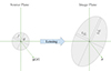Fig. 1. Lensing effect on an infinitesimally small source. Locally a source that is circularly symmetric gets lensed into an ellipse. The eigenvectors of the Jacobian of the lensing function y shown in Eq. (3) are parallel to the semiminor and semimajor axes of this ellipse. If the source has unit radius, the lengths of the semiminor and semimajor axes are given by the eigenvalues of the Jacobian.

The direction of the primary eigenvector tells us the direction along which the stretching of the source image due to lensing is maximum. If we “move” a point on the image along the direction of the primary eigenvector, the corresponding point on the source plane will move minimally. The direction in which the heavily magnified arcs appear to be stretched typically lie along the direction of the primary eigenvector, assuming that the shape of the source galaxy is not unusually elongated. We made use of this property in parameterizing our model for the angular deflection field, y.

2.2. Forming multiple images

We consider a curve, $\xi (t):ℝ\to {ℝ}^2$, which maps the coordinate t to its corresponding point on the image plane, such that at each point this curve is tangent to the primary eigenvector of the lensing function. We call any curve with this property the primary curve. We qualitatively illustrate how images lie along the primary curve in Fig. 2, where we show the lensed image of a disk-shaped source. The source is a color wheel, shown in the bottom-right subplot to make the effect of lensing clearer to see by eye. The dashed curve on the left subplot shows the primary curve which is parameterized by t. The dashed curve in the bottom-right subplot is the curve that you get when you map the primary curve onto the source plane. The blue curve in the top-right subplot shows the eigenvalue λ₁(t) as a function of the parameter t. If we start from the bottom of the primary curve and move along the curve with increasing t, we notice that initially λ₁ is positive. This means that on the source plane we also move along the same direction. As we keep moving and cross t = 0, λ₁ flips to negative. As this happens, the movement on the source plane slows down, stops, and reverses direction. This forms the first kink of the dashed curve on the source plane. Because the movement on the source plane reversed directions, it goes over the source again to form the second image which is between t = 0.00 and t = 0.75. As we cross t = 1.00, λ₁ flips back to positive, resulting in another change in direction on the source plane. This forms the other kink of the dashed curve on the source plane. We cross over the source once more to form the third image which is around t = 1.25. We can see from the color wheel pattern that the parities of the first and third image are positive and the parity of the second image is negative.

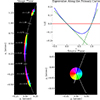Fig. 2. Qualitative illustration of lensing along a primary curve. Left: The lensed images of a disk shaped color wheel source. The dashed curve shows the primary curve ξ(t) parameterized by t. The values of t along the primary curve are shown as solid ticks. Top-right: Values of the primary eigenvalue λ1(t) along the primary curve. The places where λ1(t) hits 0 corresponds to the critical curve crossings where the magnification is infinite. Bottom-right: Unlensed image of the color wheel source. The dashed curve shows the set of points that we get when we map the primary curve onto the source plane.

2.3. Parametrization of the primary curve

We can first parameterize a lensing function and calculate its primary curves. However, in this work, we first parameterize a curve and determine this curve to be the primary curve of our lensing function.

We parameterize the primary curve with n+3 parameters (d₁,d₂,θ₀,a₁,…,a_n). As determined by these parameters, the curve is given by

$$\xi (t)=\left(\begin{array}{c}\hfill d_1\hfill \\ \hfill d_2\hfill \end{array}\right)+Q_n(t)\left(\begin{array}{c}\hfill cos{\theta }_0\hfill \\ \hfill sin{\theta }_0\hfill \end{array}\right)+P_n(t)\left(\begin{array}{c}\hfill -sin{\theta }_0\hfill \\ \hfill cos{\theta }_0\hfill \end{array}\right),$$(4)

where

$$Q_n(t)={\displaystyle {\int }_0^t}\mathrm{d}{t}^{\prime }cos{\theta }_n(t^{\prime }),$$(5)

$$P_n(t)={\displaystyle {\int }_0^t}\mathrm{d}{t}^{\prime }sin{\theta }_n(t^{\prime }),$$(6)

and

$${\theta }_n(t)=a_{1}t+a_2{t}^2+\dots +a_n{t}^n.$$(7)

We chose a coordinate basis for the neighborhood of the primary curve with the function $\zeta :{ℝ}^2\to {ℝ}^2$. Motivated by the fact that the eigenvectors of the lensing function are orthogonal, we chose

$$\zeta \left[\left(\begin{array}{c}\hfill t\hfill \\ \hfill s\hfill \end{array}\right)\right]=\xi (t)+\left(\begin{array}{cc}\hfill 0\hfill & \hfill -1\hfill \\ \hfill 1\hfill & \hfill 0\hfill \end{array}\right)\left(\frac{\mathrm{d}\xi }{\mathrm{d}t}\right)s.$$(8)

This function ζ takes in a pair of coordinates (t,s) and maps them to the corresponding point on the image plane. The first coordinate t describes how far along the primary curve the point is while the second coordinate s describes how far from the curve the point is. This is a bijective function (whose inverse we calculate in Appendix A) as long as s is smaller than the curvature radius of ξ. Using Eq. (4), we can obtain an explicit expression:

$$\zeta \left[\left(\begin{array}{c}\hfill t\hfill \\ \hfill s\hfill \end{array}\right)\right]=\left(\begin{array}{c}\hfill d_1\hfill \\ \hfill d_2\hfill \end{array}\right)+\left(Q_n(t)-s\frac{\mathrm{d}{P}_n}{\mathrm{d}t}(t)\right)\left(\begin{array}{c}\hfill cos{\theta }_0\hfill \\ \hfill sin{\theta }_0\hfill \end{array}\right)$$(9)

$$+\left(P_n(t)+s\frac{\mathrm{d}{Q}_n}{\mathrm{d}t}(t)\right)\left(\begin{array}{c}\hfill -sin{\theta }_0\hfill \\ \hfill cos{\theta }_0\hfill \end{array}\right).$$

2.4. Parametrization of the lens model

We define the transitive lensing function $\tilde{y}(u)$ as a function of $u=\left(\begin{array}{c}\hfill t\hfill \\ \hfill s\hfill \end{array}\right)$ with the following relation

$$\tilde{y}(u)\equiv y(\zeta (u)),$$(10)

where y is the lensing function defined in Eq. (1). This transitive lensing function maps our new coordinate system (t,s) to the source plane, shown in Fig. 3. It is convenient express it as an integral:

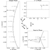Fig. 3. Flow of the lens model: Dashed line is the primary curve ξ whose parametrization is shown in Eq. (4). Given a primary curve the function ζ (shown in Eq. (9)) is a coordinate system that labels the points on the image plane with coordinates t,s. The transitive lensing function $\tilde{y}$ (defined in Eq. (10)) maps the points on the t−s plane onto the source plane. Combining $\tilde{y}$ with the inverse function ζ−1 gives us the lensing function y that maps the image plane to the source plane.

$$\tilde{y}\left[\left(\begin{array}{c}\hfill t\hfill \\ \hfill 0\hfill \end{array}\right)\right]=\tilde{y}\left[\left(\begin{array}{c}\hfill 0\hfill \\ \hfill 0\hfill \end{array}\right)\right]+{\displaystyle {\int }_0^t}\mathrm{d}{t}^{\prime }\left(\frac{\partial \tilde{y}}{\partial t^{\prime }}\right){|}_{(t^{\prime },0)},$$(11)

$$=\tilde{y}\left[\left(\begin{array}{c}\hfill 0\hfill \\ \hfill 0\hfill \end{array}\right)\right]+{\displaystyle {\int }_0^t}\mathrm{d}{t}^{\prime }\left(\frac{\partial y}{\partial x}\right){|}_{(t^{\prime },0)}\left(\frac{\partial \zeta }{\partial t^{\prime }}\right){|}_{(t^{\prime },0)},$$(12)

$$=\tilde{y}\left[\left(\begin{array}{c}\hfill 0\hfill \\ \hfill 0\hfill \end{array}\right)\right]+{\displaystyle {\int }_0^t}\mathrm{d}{t}^{\prime }\left(\frac{\partial y}{\partial x}\right){|}_{(t^{\prime },0)}\left(\frac{\mathrm{d}\xi }{\mathrm{d}{t}^{\prime }}\right).$$(13)

Now, we can make use of the fact that ξ is a primary curve, which makes $\frac{\mathrm{d}\xi }{\mathrm{d}{t}^{\prime }}$ an eigenvector of the Jacobian with the eigenvalue λ₁(t′). This leads to:

$$\tilde{y}\left[\left(\begin{array}{c}\hfill t\hfill \\ \hfill 0\hfill \end{array}\right)\right]=\tilde{y}\left[\left(\begin{array}{c}\hfill 0\hfill \\ \hfill 0\hfill \end{array}\right)\right]+{\displaystyle {\int }_0^t}\mathrm{d}{t}^{\prime }{\lambda }_1(t^{\prime })\left(\frac{\mathrm{d}\xi }{\mathrm{d}{t}^{\prime }}\right).$$(14)

We can carry out a similar integral along the secondary eigenvector, which is orthogonal to the primary eigenvector. Thus, we have:

$$\tilde{y}\left[\left(\begin{array}{c}\hfill t\hfill \\ \hfill s\hfill \end{array}\right)\right]=\tilde{y}\left[\left(\begin{array}{c}\hfill t\hfill \\ \hfill 0\hfill \end{array}\right)\right]+{\displaystyle {\int }_0^s}\mathrm{d}{s}^{\prime }\left(\frac{\partial \tilde{y}}{\partial s^{\prime }}\right){|}_{(t,s^{\prime })},$$(15)

$$=\tilde{y}\left[\left(\begin{array}{c}\hfill t\hfill \\ \hfill 0\hfill \end{array}\right)\right]+{\displaystyle {\int }_0^s}\mathrm{d}{s}^{\prime }\left(\frac{\partial y}{\partial x}\right){|}_{(t,s^{\prime })}\left(\frac{\partial \zeta }{\partial s^{\prime }}\right){|}_{(t,s^{\prime })},$$(16)

$$=\tilde{y}\left[\left(\begin{array}{c}\hfill t\hfill \\ \hfill 0\hfill \end{array}\right)\right]+{\displaystyle {\int }_0^s}\mathrm{d}{s}^{\prime }\left(\frac{\partial y}{\partial x}\right){|}_{(t,s^{\prime })}\left(\begin{array}{cc}\hfill 0\hfill & \hfill -1\hfill \\ \hfill 1\hfill & \hfill 0\hfill \end{array}\right)\left(\frac{\mathrm{d}\xi }{\mathrm{d}t}\right)·$$(17)

At s = 0, $\left(\begin{array}{cc}\hfill 0\hfill & \hfill -1\hfill \\ \hfill 1\hfill & \hfill 0\hfill \end{array}\right)\left(\frac{\mathrm{d}\xi }{\mathrm{d}t}\right)$ is an eigenvector of the Jacobian. However, at s>0 this is no longer true in general. We can Taylor expand this integral around s = 0, keeping the terms up to third order in s and we have:

$$\begin{array}{cc}\hfill \tilde{y}\left[\left(\begin{array}{c}\hfill t\hfill \\ \hfill s\hfill \end{array}\right)\right]=\tilde{y}\left[\left(\begin{array}{c}\hfill t\hfill \\ \hfill 0\hfill \end{array}\right)\right]& +s\left(\frac{\partial y}{\partial x}\right){|}_{(t,0)}\left(\begin{array}{cc}\hfill 0\hfill & \hfill -1\hfill \\ \hfill 1\hfill & \hfill 0\hfill \end{array}\right)\left(\frac{\mathrm{d}\xi }{\mathrm{d}t}\right),\hfill \\ \hfill & +\frac{s^2}{2}\left(\frac{\partial }{\partial s}\frac{\partial y}{\partial x}\right){|}_{(t,0)}\left(\begin{array}{cc}\hfill 0\hfill & \hfill -1\hfill \\ \hfill 1\hfill & \hfill 0\hfill \end{array}\right)\left(\frac{\mathrm{d}\xi }{\mathrm{d}t}\right),\hfill \\ \hfill & +\frac{s^3}{6}\left(\frac{{\partial }^2}{\partial s^2}\frac{\partial y}{\partial x}\right){|}_{(t,0)}\left(\begin{array}{cc}\hfill 0\hfill & \hfill -1\hfill \\ \hfill 1\hfill & \hfill 0\hfill \end{array}\right)\left(\frac{\mathrm{d}\xi }{\mathrm{d}t}\right),\hfill \\ \hfill & +\mathcal{O}\left[s^4\right].\hfill \end{array}$$(18)

In Appendix B, we calculate the partial derivatives of the Jacobian with respect to s in terms of the eigenvalues λ₁ and λ₂, along with the orientation angle θ, which leads to:

$$\begin{array}{cc}\hfill \tilde{y}\left[\left(\begin{array}{c}\hfill t\hfill \\ \hfill s\hfill \end{array}\right)\right]=& \tilde{y}\left[\left(\begin{array}{c}\hfill t\hfill \\ \hfill 0\hfill \end{array}\right)\right]+s{\lambda }_2(t)\left(\begin{array}{cc}\hfill 0\hfill & \hfill -1\hfill \\ \hfill 1\hfill & \hfill 0\hfill \end{array}\right)\left(\frac{\mathrm{d}\xi }{\mathrm{d}t}\right),\hfill \\ \hfill & +\frac{s^2}{2}\left({\lambda }_1(t)-{\lambda }_2(t)\right)\left(\frac{\partial \theta }{\partial s}\right){|}_{(t,0)}\left(\frac{\mathrm{d}\xi }{\mathrm{d}t}\right),\hfill \\ \hfill & +\frac{s^2}{2}\left(\frac{\partial {\lambda }_2}{\partial s}\right){|}_{(t,0)}\left(\begin{array}{cc}\hfill 0\hfill & \hfill -1\hfill \\ \hfill 1\hfill & \hfill 0\hfill \end{array}\right)\left(\frac{\mathrm{d}\xi }{\mathrm{d}t}\right),\hfill \\ \hfill & +\frac{s^3}{6}\left({\lambda }_1(t)-{\lambda }_2(t)\right)\left(\frac{{\partial }^2\theta }{\partial s^2}\right){|}_{(t,0)}\left(\frac{\mathrm{d}\xi }{\mathrm{d}t}\right),\hfill \\ \hfill & +\frac{s^3}{6}[\left(\frac{{\partial }^2{\lambda }_2}{\partial s^2}\right){|}_{(t,0)}+2({\lambda }_1(t)\hfill \\ \hfill & -{\lambda }_2(t)){\left(\frac{\partial \theta }{\partial s}\right)}^2{|}_{(t,0)}]\left(\begin{array}{cc}\hfill 0\hfill & \hfill -1\hfill \\ \hfill 1\hfill & \hfill 0\hfill \end{array}\right)\left(\frac{\mathrm{d}\xi }{\mathrm{d}t}\right),\hfill \\ \hfill & +\mathcal{O}\left[s^4\right].\hfill \end{array}$$(19)

Using Eq. (4), we can explicitly calculate the derivatives of ξ. We have the following set of functions of t that will allow us to fully parameterize our lens model:

$$(1){\theta }_n(t)\hspace{0.5em}\mathrm{is}\mathrm{given}\mathrm{by}\mathrm{Eq}.\hspace{0.5em}(5);$$(20)

$$(2){\lambda }_1(t);$$(21)

$$(3){\lambda }_2(t);$$(22)

$$(4)F(t)\equiv \left(\frac{\partial {\lambda }_2}{\partial s}\right){|}_{(t,0)};$$(23)

$$(5)G(t)\equiv \left({\lambda }_1(t)-{\lambda }_2(t)\right)\left(\frac{\partial \theta }{\partial s}\right){|}_{(t,0)};$$(24)

$$(6)H(t)\equiv \left(\frac{{\partial }^2{\lambda }_2}{\partial s^2}\right){|}_{(t,0)}+2({\lambda }_1(t)-{\lambda }_2(t)){\left(\frac{\partial \theta }{\partial s}\right)}^2{|}_{(t,0)};$$(25)

$$(7)I(t)\equiv \left({\lambda }_1(t)-{\lambda }_2(t)\right)\left(\frac{{\partial }^2\theta }{\partial s^2}\right){|}_{(t,0)}.$$(26)

Combining Eq. (19) with Eq. (14) we can succinctly write the transitive lensing function by using the following notation for the integrals and the derivatives:

$$\mathcal{S}\{f\}(t)\equiv {\displaystyle {\int }_0^t}\mathrm{d}{t}^{\prime }f(t^{\prime }),$$(27)

$$\mathcal{D}\{f\}(t)\equiv \frac{\mathrm{d}f}{\mathrm{d}t}·$$(28)

We arrive at our final expression for the transitive lensing function:

$$\begin{array}{cc}\hfill \tilde{y}\left[\left(\begin{array}{c}\hfill t\hfill \\ \hfill s\hfill \end{array}\right)\right]=& \tilde{y}\left[\left(\begin{array}{c}\hfill 0\hfill \\ \hfill 0\hfill \end{array}\right)\right]+\left(\begin{array}{cc}\hfill cos{\theta }_0\hfill & \hfill -sin{\theta }_0\hfill \\ \hfill sin{\theta }_0\hfill & \hfill cos{\theta }_0\hfill \end{array}\right),\hfill \\ \hfill & [\left(\begin{array}{c}\hfill \mathcal{S}\{{\lambda }_1\mathcal{D}\{Q_n\}\}(t)\hfill \\ \hfill \mathcal{S}\{{\lambda }_1\mathcal{D}\{P_n\}\}(t)\hfill \end{array}\right)+s{\lambda }_2(t)\left(\begin{array}{c}\hfill -\mathcal{D}\{P_n\}(t)\hfill \\ \hfill \mathcal{D}\{Q_n\}(t)\hfill \end{array}\right)\hfill \\ \hfill & +\frac{s^2}{2}F(t)\left(\begin{array}{c}\hfill -\mathcal{D}\{P_n\}(t)\hfill \\ \hfill \mathcal{D}\{Q_n\}(t)\hfill \end{array}\right)+\frac{s^2}{2}G(t)\left(\begin{array}{c}\hfill \mathcal{D}\{Q_n\}(t)\hfill \\ \hfill \mathcal{D}\{P_n\}(t)\hfill \end{array}\right)\hfill \\ \hfill & +\frac{s^3}{6}H(t)\left(\begin{array}{c}\hfill -\mathcal{D}\{P_n\}(t)\hfill \\ \hfill \mathcal{D}\{Q_n\}(t)\hfill \end{array}\right)+\frac{s^3}{6}I(t)\left(\begin{array}{c}\hfill \mathcal{D}\{Q_n\}(t)\hfill \\ \hfill \mathcal{D}\{P_n\}(t)\hfill \end{array}\right)]\hfill \\ \hfill & +\mathcal{O}\left[s^4\right].\hfill \end{array}$$(29)

However, we must additionally introduce a condition that the curl of the lensing function must vanish: ∇×y = 0. This is because the angular deflections of a gravitational lens whose extent in the line-of-sight direction is much smaller than the distance between the observer and the source can be written as the gradient of a lensing potential: α=∇Ψ. Any line-of-sight effect that will break this condition should be modeled with an extension of our model that includes a curl term. Introducing the vanishing curl condition gives us the following relations, which are calculated in Appendix C:

$$0=G(t)-\mathcal{D}\{{\lambda }_2\}(t),$$(30)

$$0=I(t)-\mathcal{D}\{F\}(t)-3G(t)\mathcal{D}\{\theta \}(t),$$(31)

$$0=\mathcal{D}\{H\}(t)+4I(t)\mathcal{D}\{\theta \}(t).$$(32)

We see that choosing a particular λ₂(t) and F(t) also determines G(t) and I(t), and also H(t) up to a constant H₀:

$$G(t)=\mathcal{D}\{{\lambda }_2\}(t),$$(33)

$$I(t)=\mathcal{D}\{F\}(t)+3G(t)\mathcal{D}\{\theta \}(t),$$(34)

$$H(t)=-4\mathcal{S}\{I\mathcal{D}\{\theta \}|(t)+H_0.$$(35)

2.5. Conceptual summary

Bright lensed arcs typically lie along curves that follow the eigenvectors of the lensing Jacobian (see Fig. 2), which we have named primary curves. We first parameterize the primary curve with a polynomial. We then build a lens model that can capture the angular deflections of a complex lens within a neighborhood of the primary curve (see Fig. 3). By parameterizing how the eigenvalues of the lensing Jacobian changes along the primary curve, we parameterize transitive lensing function $\tilde{y}$ (shown in Eq. (29)). Combining the transitive lensing function with the inverse of the coordinate basis function ζ (shown in Eq. (9)) gives us a fully parametric lens model, $y(x)=\tilde{y}\left({\zeta }^{-1}(x)\right)$.

2.6. Degeneracies

In lensing, it is never possible to directly observe the angular deflections. Instead, the data consists of pixel values of the lensed image of a background source. There can be many combinations of source light distribution and lensing functions that result in the same observed image. Therefore, gravitational lensing is known to host many degeneracies (Falco et al. 1985; Saha 2000; Saha & Williams 2006; Schneider & Sluse 2013; Liesenborgs & De Rijcke 2012).

In our lens model, if we make the following transformation λ₁→aλ₁ and λ₂→aλ₂, where a is a constant, we get $\tilde{y}\to a\tilde{y}$. This means a constant scaling of the source plane, which results in a perfect degeneracy when the source is also scaled with 1/a, which is known as the mass-sheet degeneracy (MST) in the literature (Falco et al. 1985; Gorenstein et al. 1988). Therefore, we are measuring the relative values of λ₁ and λ₂. To obtain the absolute magnifications from any local modeling, we need to add the information from the global mass modeling of the cluster that makes use of all the lensed images of background sources near the cluster.

2.7. Source light modeling

Galaxies can have complex morphologies. Using simple analytical models such as the Sersic profile (Sérsic 1963) is inadequate with respect to accurately reconstructing the source light distribution. For this reason, it is crucial in lens modeling to have source light models that are flexible enough to capture these complex shapes.

One common approach is using basis sets such as shapelets (Birrer et al. 2015), which consist of orthonormal Hermite polynomials. The complexity of a shapelet set can be controlled with the shapelet index n_max, which determines the size of the smallest features relative to the overall size of the source.

In this work, we chose to use an adaptive grid technique very similar to that of Vegetti & Koopmans (2009). Initially, the Hessian matrix, H_i, of the brightness values at each image pixel i is calculated by a finite difference method. The half of the image pixels that have a quantity of |detH|/p_i higher than the median were chosen as candidate points, where p_i is the pixel value. These candidate points were subsequently filtered such that the centers of pixels in the final set {q_i} were further from each other than l_min pixel widths. These center points are then fed into the lens model to form a set of points on the source plane: {w_i} with w_i=y(q_i). This set of points make up the vertices of a Delaunay triangulation on the source plane. Each vertex, w_i, was assigned an amplitude, c_i, which determines the surface brightness of the source at that position. For the surface brightness at a generic point on the source plane w, we first need to calculate which Delaunay triangle w is enclosed within. Then the surface brightness I_s(w) is given by a linear combination of the amplitudes (c_i,c_j,c_k) of the three vertices (w_i,w_j,w_k) of that triangle:

$$I_s(w)=c_i{D}_{\mathit{ijk}}(w),$$(36)

$$+c_j{D}_{\mathit{kij}}(w),$$(37)

$$+c_k{D}_{\mathit{jki}}(w),$$(38)

where

$$D_{\mathit{ijk}}(w)\equiv \frac{(w_1-w_{k1})(w_{j2}-w_{k2})-(w_{j1}-w_{k1})(w_2-w_{k2})}{(w_{i1}-w_{k1})(w_{j2}-w_{k2})-(w_{j1}-w_{k1})(w_{i2}-w_{k2})}·$$(39)

If a point w falls outside of any Delaunay triangle, it is assigned the surface brightness of the nearest vertex.

A set of source vertex amplitudes $c\equiv (c_1,c_2,\dots ,c_{n_s})$ fully determines source surface brightness, S_source(c), on the source plane. Subsequently, a lensing operation, ℒ(m), controlled by a set of lens model parameters represented as the vector m fully determines the surface brightness, I, on the image plane with

$$I(m;c)=\mathcal{L}(m)\{S(c)\}.$$(40)

To convert this surface brightness to an observed image reconstruction, we need convolve it with a point spread function (PSF) then subsequently sample it by a pixellated grid. We denote these operations using $\mathcal{T}$. Thus, our model reconstruction can be represented as a vector:

$$M(m;c)=\mathcal{T}\{\mathcal{L}(m)\{S(c)\}\}.$$(41)

An important property of the model reconstruction is that it is a linear function of c, i.e. ∂²M/∂c_i∂c_j = 0. For a given m there is a matrix A(m) that gives M(m;c) = A(m)c. Our data, which contain the image pixels of the lensed arc we are modeling, can also be represented as a vector, d. Solving for c is then the simple problem of minimizing the following loss function:

$${\chi }^2(c)=[d-A(m)c{]}^T{\mathrm{\Sigma }}^{-1}[d-A(m)c],$$(42)

where Σ is the covariance matrix of the data vector, assuming that the pixel errors are Gaussian. We remind that c represents the surface brightness at the vertices of the Delaunay triangulation. A negative value of any c_i would mean we have an unphysical source model as surface brightness cannot be negative. So given our data and a set of lens model parameters, the source amplitudes are given by

$$\arg \min {\chi }^2(c)\mathrm{subject}\mathrm{to}{c}_i\ge 0\forall i.$$(43)

This is a well known problem called quadratic optimization and it has many efficient solvers. We used the function scipy.optimize.nnls, based on the method developed by Bro & De Jong (1997).

We illustrate this pipeline for source reconstruction in Fig. 4. We create a simulated lensed image using the Hubble Space Telescope (HST) image of galaxy NGC 1300, which is shown in the bottom-left subplot. The simulated lensed data are shown in the top-left subplot. Following the procedure described earlier in this section, we selected a set of points {q_i} on the image plane, which are shown in the top-middle subplot as the white dots. These points are then projected onto the source plane to form the vertices of a Delaunay triangulation, which is shown in the bottom-right subplot as the white triangles. The vertex amplitudes c are calculated using Eq. (43). The bottom-right and top-middle subplots show the source surface brightness reconstruction and the image model reconstruction, respectively. Comparing the source reconstruction to the true source, we see that we are able to recover many of the features seen in the complex morphology of NGC 1300. In the top-right subplot, we show the residuals after subtracting the image reconstruction from the mock data.

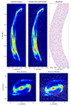Fig. 4. Source reconstruction of a mock lens. Top-left: Lensed image. Top-middle: Model reconstruction with the white points showing the source modeling points. These white dots are the points that are mapped onto the source plane to form the Delaunay triangulation vertices as described in Sect. 2.7. Top-right: Residuals after the model reconstruction is subtracted from the image. Bottom left: True source that is used in creating the mock data image. Bottom-right: Source model reconstruction with the white lines showing the Delaunay triangulation. The vertices of the triangulation are the positions after the points in the top-middle subplot are mapped onto the source plane using the lens model.

2.8. Nested sampling and Bayesian inference

The dependence of the model reconstruction M(m;c) on the lens model parameters m is highly non-linear. For each m, we set c to be the solution of Eq. (43). We can write this as M(m)≡M(m;c_min). Assuming that the pixel errors are Gaussian, we can obtain the posteriors of the model parameters using Bayesian inference:

$$P(d|m)=\frac{exp\left[-\frac{1}{2}{\left(d-M(m)\right)}^T{\mathrm{\Sigma }}^{-1}\left(d-M(m)\right)\right]}{\sqrt{(2\pi {)}^{dimd}det(\mathrm{\Sigma })}},$$(44)

$$P(m|d)=\frac{P(d|m)P(m)}{P(d)}·$$(45)

We used the nested sampling package dynesty (Speagle 2020) to sample the likelihood function to obtain the lens parameter posteriors, along with the best-fit parameters.

3. Results

3.1. SDSS J1110+6459

SDSS J1110+6459 is a galaxy cluster gravitational lens that is host to one of the most striking examples of a lensed arc, which can be seen in Fig. 3 of Johnson et al. (2017). This arc consists of three merging images of a background galaxy at z = 2.481 (Stark et al. 2013; Johnson et al. 2017). The galaxy cluster lens is at a redshift of z = 659 (Oguri et al. 2012; Stark et al. 2013; Johnson et al. 2017).

An early strong lensing analysis of SDSS J1110+6459 was performed by Oguri et al. (2012), where they used the low-resolution ground-based Subaru telescope. Without access to accurate spectroscopic redshifts, these early lens modeling efforts were poorly constrained. By using the higher-resolution HST imaging, as well as the spectroscopic redshifts for the sources, Johnson et al. (2017) provided the first high-fidelity strong lens modeling, which we used in making the parametrization choices for our lens model.

The cutout we used of the bright arc in SDSS J1110+6459 is shown in the top-left subplot of Fig. 7. The data were taken with HST/WFC3 on January 8, 2013 and made publicly available on the MAST portal¹. We used the F390W filter observation with 1212 seconds of exposure. The three images of the same source galaxy are clearly seen from the bottom to the top along our cutout. In Fig. 2, we shown another aspect that is qualitatively similar to what we have shown in this work, with respect to the arc. The primary curve lies roughly along our cutout with the primary eigenvalue λ₁ flipping signs twice as we move from the bottom of the image to the top. The first sign flip (from positive to negative) is between the first image and the second image near (−0.5″,−2.5″), which we used as an initialization of (d₁,d₂) (shown in Eq. (4)). The second sign flip is (from negative to positive) between the second image and the third image near (1.0″,5.0″).

Considering these properties, we parameterize λ₁ as a polynomial:

$$\begin{array}{cc}\hfill {\lambda }_1(t)=& r_{0}t\left(1-\frac{t}{t_{\mathrm{cr}}}\right)\left(1-\frac{t}{t_{\mathrm{cr}}}-\frac{r_{\mathrm{cr}}}{r_0}\frac{t}{t_{\mathrm{cr}}}\right)\hfill \\ \hfill & +q_4{t}^2{\left(1-\frac{t}{t_{\mathrm{cr}}}\right)}^2\left(1+q_{5}t+q_6{t}^2+\dots +q_m{t}^{m-4}\right),\hfill \end{array}$$(46)

which displays the following properties:

$$(1){\lambda }_1(0)=0,$$(47)

$$(2){\lambda }_1(t_{\mathrm{cr}})=0,$$(48)

$$(3)\frac{\mathrm{d}{\lambda }_1}{\mathrm{d}t}{|}_{t=0}=r_0,$$(49)

$$(4)\frac{\mathrm{d}{\lambda }_1}{\mathrm{d}t}{|}_{t=t_{\mathrm{cr}}}=r_{\mathrm{cr}}.$$(50)

The parameter, r₀, is the slope of λ₁ at t = 0, which has a negative value as the first sign flip is from positive to negative. The parameter t_cr is the position of the second sign flip of λ and r_cr is the slope of λ₁ at t=t_cr, which has a positive value as the second sign flip is from negative to positive. The remaining parameters q₄,…,q_m are higher order terms that allow further flexibility in λ₁, while preserving the properties in Eqs. (47)–(50). We fixed λ₂(0) = 1 due to the degeneracy described in Sect. 2.6, which means that the values we inferred in our analysis for λ₁(t) are ratios of λ₁(t)/λ₂(0).

Our lens model has the parameters for the primary curve (d₁,d₂,θ₀,a₁,…,a_n) and the parameters for the eigenvalue (t_cr,r₀,r_cr,q₄,…,q_m). To avoid overfitting the data, we need to find the optimal values for the hyperparameters n, m, and l_min, where l_min is the hyperparameter that controls the number of source modeling points. Performing a 3D grid search by simultaneously varying all three is too computationally costly, since it requires running a nested sampling for hundreds of combinations of (n,m,l_min). Therefore, we fixed the value of l_min = 4 and only vary n and m. We performed a grid search with the range n={1,2,3,4,5,6} and m∈{4,5,6,7,8,9}. For each combination of (n,m), we found the best fit using nested sampling and calculate the Bayesian information criterion (BIC), given as BIC = kln(n_pix)+χ², where n_pix is the number of unmasked pixels and k is the number of model parameters. Models with a greater number of parameters result in a higher BIC if they do not significantly improve the χ². We show these results in Fig. 5, where we find that the BIC decreases as we increase n and m. We see that the optimal (n,m) is larger than n>6 or m>9 and lies outside of our grid search range. Since higher values of n and m call for a more complicated lens model, we end up underfitting the data. Performing a grid search for higher values of n and m is also computationally costly because when n and m are large, the high dimensionality of the parameter space makes nested sampling increasingly inefficient. Improvements in the speed of ray-tracing software (possibly in the form of parallelization) are needed to fully utilize the data by using more complicated and flexible lens models.

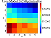Fig. 5. Grid search for the optimal n and m values for J1110+6459. The color in each pixel shows the best fit BIC value of the corresponding lens model with (n,m). Source modeling hyperparameter is fixed to lmin = 4.

To determine the optimal source modeling hyperparameter, l_min, we fixed the values of n = 6 and m = 9. Although these values are not optimal, they were found to have the smallest BIC within the range of our grid search. We then varied l_min within the range l_min={1,2,3,4,5,6,7,8,9} as we calculated the best-fit BIC. We find (as we show in Fig. 6) that l_min = 4 gives the lowest BIC. We note that lower values of l_min mean that there are fewer source modeling points. Thus, when l_min<4, the source modeling ends up overfitting the data, whereas when l_min>4, the source modeling ends up underfitting the data.

Fig. 6. Best-fit BIC for J1110+6459 as the source modeling hyperparameter lmin is varied. Lens modeling hyperparameters are fixed to n = 6 and m = 9.

We set uninformative flat priors for all the model parameters. The priors for (d₁,d₂) were chosen such that it stays between the first and the second image along the arc, as the sign flip for λ₁ needs to remain between these images. Similarly, the prior t_cr is chosen such that the second sign flip is between the second and third images along the arc. The priors for r₀ and r_cr were chosen such that the former is strictly negative and the latter is strictly positive. We calculated the posterior probabilities for the model parameters using the nested sampling package dynesty (Speagle 2020).

In Fig. 7, we show the best fit of our lens model obtained from our sampling, with the hyperparameters: n = 6, m = 9, and l_min = 4. In the top-left subplot, we show the lensed image of the bright arc. In the top-middle subplot, we show our model reconstruction. In the top-right subplot, we show the image residuals after the reconstruction is subtracted from the data. In the bottom-left subplot, we show the source reconstruction with the Delaunay triangulation shown as white lines. In the bottom left subplot we show a zoomed-in version of our source reconstruction focusing on a high magnification region.

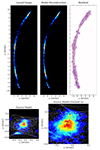Fig. 7. Image reconstruction of the bright arc in SDSS J1110+6459, with n = 6, m = 9, and lmin = 4. Top-left: Lensed image cutout of the bright arc from the HST/WFC3 UVIS F390W observation. Top-middle: Model reconstruction. Top-right: Residuals after the model reconstruction is subtracted from the data. Bottom-left: Source model reconstruction with the white lines showing the Delaunay triangulation. The vertices of the triangulation are the positions after the points in the top-middle subplot are mapped onto the source plane using the lens model. Bottom-right: Source model reconstruction zoomed in showing high magnification regions.

3.2. SDSS J0004–0103

SDSS J0004−0103 is another galaxy cluster gravitational lens that also hosts a clear lensed arc that consists of three merging images of a background galaxy at z = 1.681 (Rigby et al. 2018). An earlier lensing analysis of SDSS J0004−0103 (Sharon et al. 2020) resulted in a non-unique lens model with large systematic uncertainty due to the limited number of background sources and a lack of a dominant cluster center galaxy.

We show the cutout we use of the bright arc in SDSS J1110+6459 in the top-left subplot of Fig. 10. The data was taken with HST/WFC3 on September 24, 2013 and is publicly available on the MAST portal¹. We use the F390W filter observation with 2388 seconds of exposure. Sharon et al. (2020) has shown that the arc crosses the critical curve twice, resulting in two sign flips of λ₁. The blend of the three images is more difficult to see by eye in this system, compared to the arc described in Sect. 3.1. Therefore, we need to use the mathematical model for λ₁ given in Eq. (46).

Similarly to the process described in Sect. 3.1, to find the optimal hyperparameters n, m, and l_min, we performed a grid search. We fixed the value of l_min = 4 and varied n and m within the range n={1,2,3,4,5,6} and m∈{4,5,6,7,8,9}. For each combination of (n,m), we found the best fit using nested sampling and calculated the BIC. As we show in Fig. 8, we find that the BIC decreases as we increase n and m. Once again, we see that the optimal (n,m) is larger than n>6 or m>9 and lies outside of our grid search. Since higher values of n and m mean a more complicated lens model, we end up underfitting the data.

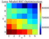Fig. 8. Grid search for the optimal n and m values for J0004−0103. The color in each pixel shows the best fit BIC value of the corresponding lens model with (n,m). The source modeling hyperparameter is fixed to lmin = 4.

To determine the optimal source modeling hyperparameter l_min, we fixed the values of n = 4 and m = 9. Although these value are not optimal, they were found to have the smallest BIC within the range of our grid search. We then varied l_min within the range of l_min={1,2,3,4,5,6,7,8,9} after finding the best-fit BIC. As we show in Fig. 9, l_min = 3 gives the lowest BIC.

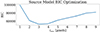Fig. 9. Best-fit BIC for J0004−0103 as the source modeling hyperparameter lmin is varied. Lens modeling hyperparameters are fixed to n = 4 and m = 9.

In Fig. 10, we show the best fit of our lens model obtained from our sampling, with the hyperparameters n = 4, m = 9, l_min = 3. In the top-left subplot, we show the lensed image of the bright arc. In the top-middle subplot we show our model reconstruction. In the top-right subplot, we show the image residuals after the reconstruction is subtracted from the data. In the bottom-left subplot, we show the source reconstruction with the Delaunay triangulation shown as white lines. In the bottom-left subplot, we show a zoomed-in version of our source reconstruction focusing on a high magnification region.

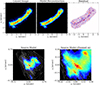Fig. 10. Image reconstruction of the bright arc in SDSS J0004−0103, with n = 4, m = 9, and lmin = 3. Top-left: Lensed image cutout of the bright arc from the HST/WFC3 UVIS F390W observation. Top-middle: Model reconstruction. Top-right: Residuals after the model reconstruction is subtracted from the data. Bottom-left: Source model reconstruction with the white lines showing the Delaunay triangulation. The vertices of the triangulation are the positions after the points in the top-middle subplot are mapped onto the source plane using the lens model. Bottom-right: The source model reconstruction zoomed in showing high-magnification regions.

4. Discussion

Bright lensed arcs provide a rare opportunity to probe structure down to 100 pc scales for high redshift galaxies. Probing these small scales offers vital information on the formation and evolution of galaxies. Having an accurate lens model near the critical curves where the magnification is highest is crucial in properly delensing the image to infer what the source looks like. The simultaneous source and lens modeling we have developed in this work allows for better source reconstructions of these bright arcs.

Global cluster lens models are shown to offer substantial benefits by utilizing the information of the extended source light distributions (Pascale et al. 2022; Bergamini et al. 2021; Diego et al. 2022; Sharon et al. 2022). Applying the constraints from the local lens model that we developed in this work for the bright arcs is just as likely to improve the fidelity of global lens models, as this approach utilizes the full information in the extended light distribution.

Our analysis shows that even with the highest level of flexibility currently achievable in our lens model, while maintaining computational tractability, we still end up underfitting the data for both systems studied in this work. This suggests that there is additional information embedded in the pixel-level data that remains untapped. To address this, parallelizing the ray-tracing calculations could provide the necessary speed improvements, enabling the use of more complex lens models and potentially uncovering more information from the data.

The lens model we use throughout this work is smooth by construction. It has the flexibility to capture complicated lensing functions, but it can only fit the slowly varying angular deflection field of the galaxy cluster. In the cold dark matter (CDM) paradigm, galaxy halos and cluster halos are expected to host a large number of low-mass subhalos (<10¹⁰ M_⊙) that do not have detectable luminosities. If properly aligned, these subhalos, along with similarly low-mass dark line-of-sight halos, create small perturbations in bright arcs with their angular deflections. In galaxy-galaxy lenses, lens modeling by fitting the pixels of the image has been shown to have the sensitivity to detect these dark perturbers down to 10⁸ M_⊙ (Vegetti et al. 2010, 2012). Recently, it has been shown that the same sensitivity can be reached in cluster lenses by locally modeling the angular deflections near the multiple images of a source (Şengül et al. 2023). By modeling the smooth component of the angular deflections of the cluster with the method that we developed in this work, we can similarly detect low-mass perturbers in cases where there are significant residuals, thereby calling for a localized mass to be added to the model. We leave this pursuit of dark substructures to future works.

Data availability

The code used for our analysis is available at https://github.com/acagansengul/alongprimarycurve

Acknowledgments

AÇŞ is supported by the Samuel P. Langley PITT PACC Postdoctoral Fellowship. AÇŞ would like to thank Simon Birrer, Cora Dvorkin, Chandrika Chandrashekar, Nino Ephremidze, and Andrew Zentner for useful discussions and comments.

References

Appendix A: Quick inversion

It is useful to also have a way to quickly invert ζ in Eq. (9) to computationally implement lensing calculations. We start with a point

$$\left(\begin{array}{c}\hfill x_1\hfill \\ \hfill x_2\hfill \end{array}\right)={\hat{x}}_1\left(\begin{array}{c}\hfill cos{\theta }_0\hfill \\ \hfill sin{\theta }_0\hfill \end{array}\right)+{\hat{x}}_2\left(\begin{array}{c}\hfill -sin{\theta }_0\hfill \\ \hfill cos{\theta }_0\hfill \end{array}\right).$$(A.1)

For a given (x₁,x₂) we can easily find $({\hat{x}}_1,{\hat{x}}_2)$. It is simply,

$${\hat{x}}_1=x_{1}cos{\theta }_0+x_{2}sin{\theta }_0$$(A.2)

$${\hat{x}}_2=x_{2}cos{\theta }_0-x_{1}sin{\theta }_0.$$(A.3)

We try to solve the inverse function ζ⁻¹ that gives,

$${\zeta }^{-1}\left[\left(\begin{array}{c}\hfill x_1\hfill \\ \hfill x_2\hfill \end{array}\right)\right]=\left(\begin{array}{c}\hfill t\hfill \\ \hfill s\hfill \end{array}\right).$$(A.4)

We can first set (t,0) and find the t that gives the nearest point. To do this, we write:

$$f(t)={\left|-\left(\begin{array}{c}\hfill x_1\hfill \\ \hfill x_2\hfill \end{array}\right)+Q_n(t)\left(\begin{array}{c}\hfill cos{\theta }_0\hfill \\ \hfill sin{\theta }_0\hfill \end{array}\right)+P_n(t)\left(\begin{array}{c}\hfill -sin{\theta }_0\hfill \\ \hfill cos{\theta }_0\hfill \end{array}\right)\right|}^2$$(A.5)

$$={\left|\left(\begin{array}{c}\hfill (Q_n(t)-{\hat{x}}_1)cos{\theta }_0-(P_n(t)-{\hat{x}}_2)sin{\theta }_0\hfill \\ \hfill (Q_n(t)-{\hat{x}}_1)sin{\theta }_0+(P_n(t)-{\hat{x}}_2)cos{\theta }_0\hfill \end{array}\right)\right|}^2$$(A.6)

$$=(Q_n(t)-{\hat{x}}_1{)}^2+(P_n(t)-{\hat{x}}_2{)}^2.$$(A.7)

Candidate solutions for the nearest point are the roots of the derivative of f(t). We calculate,

$$D\{f\}(t)=2(Q_n(t)-{\hat{x}}_1)\mathcal{D}\{Q_n\}(t)+2(P_n(t)-{\hat{x}}_2)\mathcal{D}\{P_n\}(t).$$(A.8)

Among the roots of D{f}, we select the t_min that gives the minimum f(t_min). This root finding is quickly done with Newton's method by iterating:

$$t_0=0,$$(A.9)

$$t_{i+1}=t_i-\frac{\mathcal{D}\{f\}(t_i)}{\mathcal{DD}\{f\}(t_i)}.$$(A.10)

We find that i = 10 gives the desired accuracy of |t_min−t_i|<10⁻⁸. Once this root is found, the value of s is simply given by

$$s=\frac{{\hat{x}}_2-P_n(t_{\min })}{\mathcal{D}\{Q_n\}(t_{\min })}=-\frac{{\hat{x}}_1-Q_n(t_{\min })}{\mathcal{D}\{P_n\}(t_{\min })},$$(A.11)

whichever is not singular.

Appendix B: Secondary eigenvector approximation

To calculate the transitive lensing function for larger s, we start by writing all the terms of Eq. (17) up to s³:

$$\tilde{y}\left[\left(\begin{array}{c}\hfill t\hfill \\ \hfill s\hfill \end{array}\right)\right]=\tilde{y}\left[\left(\begin{array}{c}\hfill 0\hfill \\ \hfill 0\hfill \end{array}\right)\right]+{\displaystyle {\int }_0^t}{\mathit{dt}}^{\prime }{\lambda }_1(t^{\prime })\left(\frac{d\xi }{{\mathit{dt}}^{\prime }}\right)$$(B.1)

$$\begin{array}{cc}\hfill & +{\displaystyle {\int }_0^s}{\mathit{ds}}^{\prime }\left(\frac{\partial y}{\partial x}\right)\left(\begin{array}{cc}\hfill 0\hfill & \hfill -1\hfill \\ \hfill 1\hfill & \hfill 0\hfill \end{array}\right)\left(\frac{d\xi }{\mathit{dt}}\right)\hfill \\ \hfill & =\tilde{y}\left[\left(\begin{array}{c}\hfill 0\hfill \\ \hfill 0\hfill \end{array}\right)\right]+{\displaystyle {\int }_0^t}{\mathit{dt}}^{\prime }{\lambda }_1(t^{\prime })\left(\frac{d\xi }{{\mathit{dt}}^{\prime }}\right)\hfill \\ \hfill & +s\left(\frac{\partial y}{\partial x}\right){|}_{(t,0)}\left(\begin{array}{cc}\hfill 0\hfill & \hfill -1\hfill \\ \hfill 1\hfill & \hfill 0\hfill \end{array}\right)\left(\frac{d\xi }{\mathit{dt}}\right)\hfill \\ \hfill & +\frac{s^2}{2}\left(\frac{\partial }{\partial s}\frac{\partial y}{\partial x}\right){|}_{(t,0)}\left(\begin{array}{cc}\hfill 0\hfill & \hfill -1\hfill \\ \hfill 1\hfill & \hfill 0\hfill \end{array}\right)\left(\frac{d\xi }{\mathit{dt}}\right)\hfill \\ \hfill & +\frac{s^3}{6}\left(\frac{{\partial }^2}{\partial s^2}\frac{\partial y}{\partial x}\right){|}_{(t,0)}\left(\begin{array}{cc}\hfill 0\hfill & \hfill -1\hfill \\ \hfill 1\hfill & \hfill 0\hfill \end{array}\right)\left(\frac{d\xi }{\mathit{dt}}\right)+\mathcal{O}\left[s^4\right].\hfill \end{array}$$(B.2)

Using Eq. (3) we calculate the partial derivative:

$$\begin{array}{cc}\hfill \left(\frac{\partial }{\partial s}\frac{\partial y}{\partial x}\right)=& \frac{\partial \theta }{\partial s}\left(\begin{array}{cc}\hfill -sin\theta \hfill & \hfill -cos\theta \hfill \\ \hfill cos\theta \hfill & \hfill -sin\theta \hfill \end{array}\right)\left(\begin{array}{cc}\hfill {\lambda }_1\hfill & \hfill \hfill \\ \hfill \hfill & \hfill {\lambda }_2\hfill \end{array}\right)\left(\begin{array}{cc}\hfill cos\theta \hfill & \hfill sin\theta \hfill \\ \hfill -sin\theta \hfill & \hfill cos\theta \hfill \end{array}\right)\hfill \\ \hfill & +\left(\begin{array}{cc}\hfill cos\theta \hfill & \hfill -sin\theta \hfill \\ \hfill sin\theta \hfill & \hfill cos\theta \hfill \end{array}\right)\left(\begin{array}{cc}\hfill \frac{\partial {\lambda }_1}{\partial s}\hfill & \hfill \hfill \\ \hfill \hfill & \hfill \frac{\partial {\lambda }_2}{\partial s}\hfill \end{array}\right)\left(\begin{array}{cc}\hfill cos\theta \hfill & \hfill sin\theta \hfill \\ \hfill -sin\theta \hfill & \hfill cos\theta \hfill \end{array}\right)\hfill \\ \hfill & +\frac{\partial \theta }{\partial s}\left(\begin{array}{cc}\hfill cos\theta \hfill & \hfill -sin\theta \hfill \\ \hfill sin\theta \hfill & \hfill cos\theta \hfill \end{array}\right)\left(\begin{array}{cc}\hfill {\lambda }_1\hfill & \hfill \hfill \\ \hfill \hfill & \hfill {\lambda }_2\hfill \end{array}\right)\left(\begin{array}{cc}\hfill -sin\theta \hfill & \hfill cos\theta \hfill \\ \hfill -cos\theta \hfill & \hfill -sin\theta \hfill \end{array}\right).\hfill \end{array}$$(B.3)

As this matrix appears in the calculation as being applied to $\left(\begin{array}{cc}\hfill 0\hfill & \hfill -1\hfill \\ \hfill 1\hfill & \hfill 0\hfill \end{array}\right)\left(\begin{array}{c}\hfill cos\theta \hfill \\ \hfill sin\theta \hfill \end{array}\right)$ we calculate:

$$\begin{array}{cc}\hfill \left(\frac{\partial }{\partial s}\frac{\partial y}{\partial x}\right)\left(\begin{array}{c}\hfill -sin\theta \hfill \\ \hfill cos\theta \hfill \end{array}\right)& =\frac{\partial \theta }{\partial s}\left(\begin{array}{cc}\hfill -sin\theta \hfill & \hfill -cos\theta \hfill \\ \hfill cos\theta \hfill & \hfill -sin\theta \hfill \end{array}\right)\left(\begin{array}{cc}\hfill {\lambda }_1\hfill & \hfill \hfill \\ \hfill \hfill & \hfill {\lambda }_2\hfill \end{array}\right)\left(\begin{array}{c}\hfill 0\hfill \\ \hfill 1\hfill \end{array}\right)\hfill \\ \hfill & +\left(\begin{array}{cc}\hfill cos\theta \hfill & \hfill -sin\theta \hfill \\ \hfill sin\theta \hfill & \hfill cos\theta \hfill \end{array}\right)\left(\begin{array}{cc}\hfill \frac{\partial {\lambda }_1}{\partial s}\hfill & \hfill \hfill \\ \hfill \hfill & \hfill \frac{\partial {\lambda }_2}{\partial s}\hfill \end{array}\right)\left(\begin{array}{c}\hfill 0\hfill \\ \hfill 1\hfill \end{array}\right)\hfill \\ \hfill & +\frac{\partial \theta }{\partial s}\left(\begin{array}{cc}\hfill cos\theta \hfill & \hfill -sin\theta \hfill \\ \hfill sin\theta \hfill & \hfill cos\theta \hfill \end{array}\right)\left(\begin{array}{cc}\hfill {\lambda }_1\hfill & \hfill \hfill \\ \hfill \hfill & \hfill {\lambda }_2\hfill \end{array}\right)\left(\begin{array}{c}\hfill 1\hfill \\ \hfill 0\hfill \end{array}\right)\hfill \end{array}$$(B.4)

$$\begin{array}{cc}\hfill & =\frac{\partial \theta }{\partial s}\left(\begin{array}{cc}\hfill -sin\theta \hfill & \hfill -cos\theta \hfill \\ \hfill cos\theta \hfill & \hfill -sin\theta \hfill \end{array}\right)\left(\begin{array}{c}\hfill 0\hfill \\ \hfill {\lambda }_2\hfill \end{array}\right)\hfill \\ \hfill & +\left(\begin{array}{cc}\hfill cos\theta \hfill & \hfill -sin\theta \hfill \\ \hfill sin\theta \hfill & \hfill cos\theta \hfill \end{array}\right)\left(\begin{array}{c}\hfill 0\hfill \\ \hfill \hfill \\ \hfill \frac{\partial {\lambda }_2}{\partial s}\hfill \end{array}\right)\hfill \\ \hfill & +\frac{\partial \theta }{\partial s}\left(\begin{array}{cc}\hfill cos\theta \hfill & \hfill -sin\theta \hfill \\ \hfill sin\theta \hfill & \hfill cos\theta \hfill \end{array}\right)\left(\begin{array}{c}\hfill {\lambda }_1\hfill \\ \hfill 0\hfill \end{array}\right)\hfill \end{array}$$(B.5)

$$=\left({\lambda }_1-{\lambda }_2\right)\frac{\partial \theta }{\partial s}\left(\begin{array}{c}\hfill cos\theta \hfill \\ \hfill sin\theta \hfill \end{array}\right)+\frac{\partial {\lambda }_2}{\partial s}\left(\begin{array}{c}\hfill -sin\theta \hfill \\ \hfill cos\theta \hfill \end{array}\right).$$(B.6)

We can do the same calculation for the second derivative which gives us

$$\left(\frac{{\partial }^2}{\partial s^2}\frac{\partial y}{\partial x}\right)\left(\begin{array}{c}\hfill -sin\theta \hfill \\ \hfill cos\theta \hfill \end{array}\right)=\left[\left(\frac{{\partial }^2\theta }{\partial s^2}\right)\left({\lambda }_1-{\lambda }_2\right)\right]\left(\begin{array}{c}\hfill cos\theta \hfill \\ \hfill sin\theta \hfill \end{array}\right)$$(B.7)

$$+\left[2{\left(\frac{\partial \theta }{\partial s}\right)}^2\left({\lambda }_1-{\lambda }_2\right)+\frac{{\partial }^2{\lambda }_2}{\partial s^2}\right]\left(\begin{array}{c}\hfill -sin\theta \hfill \\ \hfill cos\theta \hfill \end{array}\right).$$(B.8)

Appendix C: Enforcing a vanishing curl

To calculate the conditions for y to have a vanishing curl, we start by writing the Jacobian of the lensing function. We use the chain rule for multivariate functions:

$$\frac{\partial y}{\partial x}=\left[\frac{\partial \tilde{y}}{\partial u}\right]\left[\frac{\partial u}{\partial x}\right]=\left[\frac{\partial \tilde{y}}{\partial u}\right]{\left[\frac{\partial x}{\partial u}\right]}^{-1}$$(C.1)

$$=\frac{1}{\frac{\partial x_1}{\partial t}\frac{\partial x_2}{\partial s}-\frac{\partial x_1}{\partial s}\frac{\partial x_2}{\partial t}}\left(\begin{array}{cc}\hfill \frac{\partial {\tilde{y}}_1}{\partial t}\hfill & \hfill \frac{\partial {\tilde{y}}_1}{\partial s}\hfill \\ \hfill \hfill & \hfill \hfill \\ \hfill \frac{\partial {\tilde{y}}_2}{\partial t}\hfill & \hfill \frac{\partial {\tilde{y}}_2}{\partial s}\hfill \end{array}\right)\left(\begin{array}{cc}\hfill \frac{\partial x_2}{\partial s}\hfill & \hfill -\frac{\partial x_1}{\partial s}\hfill \\ \hfill \hfill & \hfill \hfill \\ \hfill -\frac{\partial x_2}{\partial t}\hfill & \hfill \frac{\partial x_1}{\partial t}\hfill \end{array}\right).$$(C.2)

We see that the curl is proportional to

$$\nabla \times y\propto \frac{\partial \tilde{y}}{\partial s}·\frac{\partial x}{\partial t}-\frac{\partial \tilde{y}}{\partial t}·\frac{\partial x}{\partial s}.$$(C.3)

Using Eq. (9) and (29) to calculate the partial derivatives, we see that a vanishing curl implies:

$$\nabla \times y=0\Rightarrow 0=G(t)-\mathcal{D}\{{\lambda }_2\}(t)$$(C.4)

and

$$\nabla \times y=0\Rightarrow 0=-\mathcal{D}\left\{F\right\}(t)-3G(t)\mathcal{D}\{{\theta }_n\}(t).$$(C.5)

We see that we are not free to choose G(t) or F(t). They are constrained by our choice of λ₂(t). Combining Eq. (C.4) and (C.5) gives us the following solutions for G and F:

$$G(t)=\mathcal{D}\{{\lambda }_2\}(t)$$(C.6)

$$F(t)=-3\mathcal{S}\{\mathcal{D}\{{\lambda }_2\}\mathcal{D}\{{\theta }_n\}\}(t)+F_0$$(C.7)

where F₀ is a constant that represents the second partial derivative of λ₂ at t = 0 with respect to s.

Appendix D: Properties of the lens model

D.1. Magnification

We calculate the inverse magnification of our model as a function of (t,s):

$$\frac{1}{\mu }=det\left[\frac{\partial y}{\partial x}\right]=\frac{det\left[\frac{\partial y}{\partial u}\right]}{det\left[\frac{\partial x}{\partial u}\right]}$$(D.1)

References

- Adamo, A., Bradley, L. D., Vanzella, E., et al. 2024, Nature, 632, 513 [NASA ADS] [CrossRef] [Google Scholar]
- Bergamini, P., Rosati, P., Mercurio, A., et al. 2019, A&A, 631, A130 [NASA ADS] [CrossRef] [EDP Sciences] [Google Scholar]
- Bergamini, P., Rosati, P., Vanzella, E., et al. 2021, A&A, 645, A140 [EDP Sciences] [Google Scholar]
- Birrer, S. 2021, ApJ, 919, 38 [NASA ADS] [CrossRef] [Google Scholar]
- Birrer, S., Amara, A., & Refregier, A. 2015, ApJ, 813, 102 [Google Scholar]
- Bro, R., & De Jong, S. 1997, J. Chemom., 11, 393 [CrossRef] [Google Scholar]
- Caminha, G. B., Grillo, C., Rosati, P., et al. 2016, A&A, 587, A80 [NASA ADS] [CrossRef] [EDP Sciences] [Google Scholar]
- Caminha, G. B., Rosati, P., Grillo, C., et al. 2019, A&A, 632, A36 [NASA ADS] [CrossRef] [EDP Sciences] [Google Scholar]
- Chen, W., Kelly, P. L., Diego, J. M., et al. 2019, ApJ, 881, 8 [NASA ADS] [CrossRef] [Google Scholar]
- Chen, W., Kelly, P. L., Oguri, M., et al. 2022, Nature, 611, 256 [NASA ADS] [CrossRef] [Google Scholar]
- Diego, J. M., Pascale, M., Kavanagh, B. J., et al. 2022, A&A, 665, A134 [NASA ADS] [CrossRef] [EDP Sciences] [Google Scholar]
- Diego, J. M., Meena, A. K., Adams, N. J., et al. 2023a, A&A, 672, A3 [NASA ADS] [CrossRef] [EDP Sciences] [Google Scholar]
- Diego, J. M., Sun, B., Yan, H., et al. 2023b, A&A, 679, A31 [NASA ADS] [CrossRef] [EDP Sciences] [Google Scholar]
- Falco, E. E., Gorenstein, M. V., & Shapiro, I. I. 1985, ApJ, 289, L1 [Google Scholar]
- Frye, B. L., Pascale, M., Pierel, J., et al. 2024, ApJ, 961, 171 [NASA ADS] [CrossRef] [Google Scholar]
- Furtak, L. J., Meena, A. K., Zackrisson, E., et al. 2023, MNRAS, 527, L7 [Google Scholar]
- Gorenstein, M. V., Falco, E. E., & Shapiro, I. I. 1988, ApJ, 327, 693 [Google Scholar]
- Johnson, T. L., Sharon, K., Gladders, M. D., et al. 2017, ApJ, 843, 78 [NASA ADS] [CrossRef] [Google Scholar]
- Kaurov, A. A., Dai, L., Venumadhav, T., Miralda-Escudé, J., & Frye, B. 2019, ApJ, 880, 58 [NASA ADS] [CrossRef] [Google Scholar]
- Kelly, P. L., Rodney, S. A., Treu, T., et al. 2015, Science, 347, 1123 [Google Scholar]
- Kelly, P. L., Diego, J. M., Rodney, S., et al. 2018, Nat. Astron., 2, 334 [NASA ADS] [CrossRef] [Google Scholar]
- Liesenborgs, J., & De Rijcke, S. 2012, MNRAS, 425, 1772 [CrossRef] [Google Scholar]
- Meena, A. K., Zitrin, A., Jiménez-Teja, Y., et al. 2023, ApJ, 944, L6 [NASA ADS] [CrossRef] [Google Scholar]
- Meneghetti, M., Natarajan, P., Coe, D., et al. 2017, MNRAS, 472, 3177 [Google Scholar]
- Monna, A., Seitz, S., Geller, M. J., et al. 2017, MNRAS, 465, 4589 [Google Scholar]
- Oguri, M., Bayliss, M. B., Dahle, H., et al. 2012, MNRAS, 420, 3213 [Google Scholar]
- Pascale, M., Frye, B. L., Diego, J., et al. 2022, ApJ, 938, L6 [NASA ADS] [CrossRef] [Google Scholar]
- Pierel, J. D. R., Newman, A. B., Dhawan, S., et al. 2024, ApJ, 967, L37 [NASA ADS] [CrossRef] [Google Scholar]
- Rigby, J. R., Bayliss, M. B., Sharon, K., et al. 2018, AJ, 155, 104 [Google Scholar]
- Rodney, S. A., Brammer, G. B., Pierel, J. D. R., et al. 2021, Nat. Astron., 5, 1118 [NASA ADS] [CrossRef] [Google Scholar]
- Saha, P. 2000, AJ, 120, 1654 [Google Scholar]
- Saha, P., & Williams, L. L. R. 2006, ApJ, 653, 936 [NASA ADS] [CrossRef] [Google Scholar]
- Schneider, P., & Sluse, D. 2013, A&A, 559, A37 [NASA ADS] [CrossRef] [EDP Sciences] [Google Scholar]
- Schneider, P., Ehlers, J., & Falco, E. E. 1992, Gravitational Lenses (New York: Springer-Verlag) [Google Scholar]
- Şengül, A. Ç., Birrer, S., Natarajan, P., & Dvorkin, C. 2023, MNRAS, 526, 2525 [Google Scholar]
- Sérsic, J. L. 1963, Boletin de la Asociacion Argentina de Astronomia La Plata Argentina, 6, 41 [Google Scholar]
- Sharon, K., Bayliss, M. B., Dahle, H., et al. 2020, ApJS, 247, 12 [CrossRef] [Google Scholar]
- Sharon, K., Mahler, G., Rivera-Thorsen, T. E., et al. 2022, ApJ, 941, 203 [NASA ADS] [CrossRef] [Google Scholar]
- Speagle, J. S. 2020, MNRAS, 493, 3132 [Google Scholar]
- Stark, D. P., Auger, M., Belokurov, V., et al. 2013, MNRAS, 436, 1040 [Google Scholar]
- Vegetti, S., & Koopmans, L. V. E. 2009, MNRAS, 392, 945 [Google Scholar]
- Vegetti, S., Koopmans, L. V. E., Bolton, A., Treu, T., & Gavazzi, R. 2010, MNRAS, 408, 1969 [Google Scholar]
- Vegetti, S., Lagattuta, D. J., McKean, J. P., et al. 2012, Nature, 481, 341 [NASA ADS] [CrossRef] [Google Scholar]
- Welch, B., Coe, D., Diego, J. M., et al. 2022a, Nature, 603, 815 [NASA ADS] [CrossRef] [Google Scholar]
- Welch, B., Coe, D., Zackrisson, E., et al. 2022b, ApJ, 940, L1 [NASA ADS] [CrossRef] [Google Scholar]