| Issue |
A&A
Volume 699, July 2025
|
|
|---|---|---|
| Article Number | A328 | |
| Number of page(s) | 19 | |
| Section | Extragalactic astronomy | |
| DOI | https://doi.org/10.1051/0004-6361/202452457 | |
| Published online | 21 July 2025 | |
Reconstructing galaxy star formation histories from COSMOS2020 photometry using simulation-based inference
1
CNRS and Sorbonne Université, UMR 7095, Institut d’Astrophysique de Paris, 98 bis, Boulevard Arago, F-75014 Paris, France
2
Aix Marseille Univ., CNRS, CNES, LAM, Marseille, France
⋆ Corresponding author.
Received:
1
October
2024
Accepted:
28
April
2025
Abstract
We propose a novel method for reconstructing the full posterior distribution of the star formation histories (SFHs) of galaxies from broad-band photometry. Our method combines the simulation-based inference (SBI) framework using a neural network trained with SFHs and photometry from the HORIZON-AGN hydrodynamical cosmological simulation. We applied our technique for reconstructing SFHs in the COSMOS Treasury field using only COSMOS2020 photometry in the redshift range 0<z<3. The method is able to accurately estimate the SFH and quantify the Bayesian uncertainty on simulated data, with an unbiased posterior mean, σerr≤0.16 dex for all formation times and properly calibrated posterior intervals. Our SFHs broadly agree with literature measurements derived by different methods using combined photometric and spectroscopic datasets. The SFHs of galaxies as a function of location in the near-UV−r versus r−J colour-colour diagram agree in general with expectations. They vary smoothly from star-forming to passive and quiescent galaxies that are properly localised in the red part of the diagram. We extracted summary statistics to quantify the shape of the SFH, the number of peaks, and the formation redshift. The slopes of the SFHs of passive galaxies show only a weak trend with stellar mass at z<1.35 but a significant scatter, indicating that factors other than mass might drive the suppression of star-formation. Nevertheless, star-forming galaxies show a clearly mass-dependent SFH, with lower-mass galaxies undergoing more vigorous recent star-formation. Overall, the SFH slopes in COSMOS vary over a wider range than in HORIZON-AGN. Low-mass galaxies have more peaks in their mass assembly histories than high-mass galaxies, and the trend is clearer in COSMOS than in HORIZON-AGN. At a given mass, we find many different formation redshifts, but the mass dependence on the formation redshifts is weak for passive galaxies. Most passive galaxies with a stellar mass log M*/M⊙>9 had a first event of mass assembly around z∼3 (2.2<z<5.8), regardless of their mass. This work represents a pilot study for the future analysis of the Euclid Deep fields that will reach similar depths in a similar set of photometric bands, but with an area that is larger by more than an order of magnitude. This opens the possibility of deriving SFHs for millions of galaxies in a robust manner.
Key words: methods: data analysis / surveys / galaxies: evolution / galaxies: formation / large-scale structure of Universe
© The Authors 2025
 Open Access article, published by EDP Sciences, under the terms of the Creative Commons Attribution License (https://creativecommons.org/licenses/by/4.0), which permits unrestricted use, distribution, and reproduction in any medium, provided the original work is properly cited.
This article is published in open access under the Subscribe to Open model. This email address is being protected from spambots. You need JavaScript enabled to view it. to support open access publication.
1. Introduction
With the new avalanche of wide and deep astronomical surveys such as ESA's Euclid survey (Laureijs et al. 2011), astronomers now face the increasingly difficult challenge to integrate the many pieces of the galaxy formation puzzle into a comprehensive model. The question is how a consistent scenario of the galaxy evolution can be built. One of the difficulties is that it is impossible to observe the evolution of a given galaxy: The best we can do is to consider galaxy populations at different cosmic times and then try to connect them with physical models. For example, the evolution of the mass functions of passive and star-forming galaxy populations classified from a colour-colour diagram is a first-order approach to understand the rise and quenching of star formation in the Universe (e.g. Peng et al. 2010; Madau & Dickinson 2014; Santini et al. 2022; Weaver et al. 2023; Gould et al. 2023, amongst others). In this approach, only the mass and star formation rate of the galaxies at the observation redshift is considered. Galaxies with potentially different star formation and quenching histories are mixed, which makes the physical interpretation of the mass function evolution difficult.
Galaxy spectra are the cumulative emission and absorption of the many stellar populations that constitute them. These populations have various ages and metallicities depending on their formation times and conditions, and they are susceptible to imprint specific signatures on galaxy spectra. Therefore, the build-up history of galaxies is encoded in their photometry to some extent. A technique for automatically extracting individual star formation histories (SFHs) from photometric data could be a revolutionary way to improve our understanding of the galaxy formation and mass build-up in the Universe. This would allow us to sort galaxies not only by their mass and star formation rates, but also to use specific metrics based on the SFH (e.g. the formation redshift, the number of bursts, and the slope of the SFHs in their recent history), which are more directly connected to the signature of physical processes that affect galaxy histories, such as feedback and environment. Unfortunately, it has always been challenging to systematically reconstruct these histories from broad-band photometry alone with the commonly used template-fitting codes that were originally designed to estimate the photometric redshift (e.g. LePHARE; Arnouts et al. 2002; Ilbert et al. 2006, EAZY; Brammer et al. 2008 amongst others). Even the reconstruction of the recent star formation rate is questionable from fitting the standard spectral energy distribution (SED) (e.g. Laigle et al. 2019) because computing SFHs from large photometry datasets with an intermediate to low signal-to-noise ratio (S/N) is limited by the sparsity of the model set. Furthermore, large samples of photometric measurements often only have a few broad-band filters. It is therefore a key issue to optimally exploit the entirety of the information contained in broad-band colours while fitting physically motivated SFH models.
To improve the results of these classical template-fitting codes, the size of the template library might be increased by generating SEDs from many different SFHs through a more sophisticated parametrisation (e.g. Pacifici et al. 2016a; Heavens et al. 2000; Tojeiro et al. 2007). These techniques are computationally expensive, however, and cannot be blindly applied to billions of galaxies. In addition, it is challenging to choose the correct models because it significantly impacts the inference, and justifying the choice of one model over another is problematic. Another exploration avenue to be mentioned involves simpler analytical forms that are optimised to track only specific features in SFHs using photometry with a high S/N. Although efficient, these methods lack generality by design because they are limited to the identification of specific populations, such as those that undergo a recent dramatic event (e.g. Ciesla et al. 2018; Aufort et al. 2020).
To circumvent the difficulties inherent to the use of parametric SFH models (see also Carnall et al. 2019), some authors have explored the use of non-parametric SFHs that can be implemented in SED-fitting codes (e.g. Prospector Johnson & Leja 2017 or CIGALE Boquien et al. 2019), as presented by Iyer et al. (2019), Tacchella et al. (2022a), Ciesla et al. (2024), Wan et al. (2024), or Arango et al. (in prep.), for example. In general, these methods outperform traditional parametric methods, but are still inevitably dependent on the choice of the prior (e.g. continuous or stochastic) for the non-parametric model (Leja et al. 2019; Suess et al. 2022). In this context, machine-learning approaches have also gained momentum because they can optimally exploit all information contained in multidimensional datasets. Moreover, recent advances in statistical machine-learning techniques (Papamakarios et al. 2016) formalised the link between machine-learning methods and Bayesian inference.
We propose a new technique for bypassing the limitations of traditional SED-fitting approaches by using a simulation-based inference (SBI) framework to reconstruct the SFHs of galaxies. Our technique relies on the hydrodynamical cosmological simulation HORIZON-AGN (Dubois et al. 2014) as a realistic SFH model. Our model can be parametrised in a very flexible and effective way, from which Bayesian inference can be performed to estimate the SFH of a galaxy using photometry alone. For our photometric data, we used the COSMOS2020 photometric catalogue (Weaver et al. 2022), which draws on the vast amount of photometric data present in the COSMOS field (Scoville et al. 2007). COSMOS also contains spectroscopic data that we can use as an independent validation of our method.
The Euclid mission (Laureijs et al. 2011; Euclid Collaboration: Mellier et al. 2025a) promises to revolutionise not only our knowledge of the cosmological model in the future, but also models of galaxy formation and evolution. The Euclid survey, now underway since February 2024, will comprise a ∼15 000 deg2 wide survey (Euclid Collaboration: Scaramella et al. 2022a) together with a deep survey with 40 times the exposure of the wide survey. These Euclid deep fields will crucially contain very deep near-infrared photometry from the Euclid Near-Infrared Spectrograph instrument (Laureijs et al. 2011; Euclid Collaboration: Scaramella et al. 2022a; Euclid Collaboration: Mellier et al. 2025a), optical data from the Hyper-Suprime-Cam on Subaru (Euclid Collaboration: McPartland et al. 2025b), and infrared data from the Spitzer IRAC camera (Euclid Collaboration: Moneti et al. 2022b). These data represent the only survey, current or planned, that is capable of creating samples selected based on stellar mass at these depths and in these areas. These data will be an ideal sample for investigating galaxy SFHs in different populations and for probing the currently unexplored populations. In turn, we will be able to determine what triggers dramatic changes in galactic SFHs, when each of these processes occurs, and where in the large-scale structure they are most efficient at transforming galaxies. One of the primary objectives of this paper is to understand how well SFHs can be reconstructed with a photometry similar to that of the Euclid deep fields. We note that the filter set we used is slightly different from the filter set that is used on the Euclid deep fields, but our aim is not to determine the optimal filter set for the SFH reconstruction. We instead wish to demonstrate that this reconstruction is possible from photometry with a limited number of filters.
Section 2 presents our photometric catalogue together with the cosmological simulation we used as a model for the SFH inference. Section 3 describes our SBI method. In Section 4 we present our results and consistency checks with the simulations and with recent work from the literature. Section 5 highlights caveats and perspectives. Our conclusions are presented in Section 6.
We used the WMAP7 cosmology (Komatsu 2011) for our inference pipeline (as was used in HORIZON-AGN). In COSMOS, galaxy properties were estimated by LePHARE assuming the Planck13 cosmology (Planck Collaboration XVI 2014), but the effect of changing the cosmology is not significant considering the other sources of uncertainties. We used AB magnitudes (Oke & Gunn 1983) throughout.
2. Data and model
2.1. Observations, photometry, and photometric redshifts
The COSMOS field has one of the most extensive multi-wavelength coverages of any extragalactic survey. We used a subset of the rich COSMOS photometry with the aim of approximating the filter set and depths that will be available in the Euclid deep survey. Specifically, we restricted ourselves to u* from the CLAUDS survey (Sawicki et al. 2019), g, r i, and z from HSC, Y, J, H, and Ks from UltraVISTA (McCracken et al. 2012).
Our photometric measurements come from the CLASSIC version of the COSMOS2020 catalogue (Weaver et al. 2022). This catalogue uses SExtractor (Bertin & Arnouts 1996) to measure galaxy colours in 2″ apertures. The photometry reaches a 3σ depth of 28.1 mag and 25.3 in 2″ apertures in the g and Ks bands, respectively. We limited our sample at S/N>2 in the Ks band, and we restricted ourselves to the z<3 redshift range. This ensured that the available photometric set was relatively homogeneous over the optical rest frame. Finally, only objects within the unmasked area1 were kept in the sample. In addition, by design, objects without photometry in at least one of the bands were removed from the sample. The total area after conservative masking was 1.27 deg2 (Weaver et al. 2022). The final area was covered in HSC and UltraVISTA and was not affected by artefacts or bright stars.
For the analysis of our reconstructed SFHs (but not for their reconstruction), we relied on photometric redshifts, stellar masses, and absolute magnitudes derived from an SED fitting with LePHARE over the COSMOS photometric bands (Arnouts et al. 2002; Ilbert et al. 2006) using the same configuration as Ilbert et al. (2013). As an example of the performance of this code in our sample, the precision and fraction of outliers of photometric redshifts is better than 1% in the brightest bin i<22.5, and it is still ∼4% in the faintest bin 25<i<27, with a fraction of outliers of ∼20%.
2.2. Galaxy classification
An important aim of this paper is to investigate the dependence of the SFH on stellar mass and star-forming types by subdividing the parent population according to these properties (see Section 4). To do this, we relied on the physical parameters in the COSMOS2020 catalogue. First, masses were those derived from the LePHARE SED fitting. The systematic errors in galaxy masses derived in this way are generally small, below ∼0.15 dex, and the scatter is generally smaller than ∼0.1 dex (Laigle et al. 2019). We also classified galaxies as passive or star forming based on their location in the near-UV (NUV)−r versus r−J colour-colour diagram (Ilbert et al. 2013). Based on the photometric redshift of a galaxy, the rest-frame magnitudes were estimated using LePHARE while relying on the apparent magnitude that probes the part of the galaxy spectrum that is the closest to the rest-frame filter. This approach allowed us to minimise the impact of the k-correction (Ilbert et al. 2005).
2.3. The model: The HORIZON-AGN simulation
The HORIZON-AGN simulation2 (Dubois et al. 2014) is a cosmological hydrodynamical simulation run in a (100 h−1 Mpc)3 box with the adaptive mesh-refinement code ramses (Teyssier 2002). It adopts a ΛCDM cosmology with a total matter density Ωm = 0.272, a dark energy density ΩΛ = 0.728, a matter power spectrum amplitude σ8 = 0.81, a baryon density Ωb = 0.045, a Hubble constant H0 = 70.4 km s−1 Mpc−1, and ns = 0.967 compatible with the WMAP-7 data (Komatsu 2011). The initially coarse 10243 grid was adaptively refined based on the density down to one physical kiloparsec. The volume contained 10243 dark matter particles, which corresponds to a dark matter mass resolution of MDM,res = 8×10⁷ M⊙. When it was generated, HORIZON-AGN implemented our then most advanced knowledge of galaxy physics, which still holds now, including gas cooling and heating, star formation and stellar feedback, black hole formation, growth, and feedback from active galactic nuclei (Dubois et al. 2014). In similar mass and redshift ranges, measurements from HORIZON-AGN agree relatively well with observed cosmic SFH and with mass and luminosity functions.
However, some difficult-to-resolve discrepancies remain. In particular, low-mass simulated galaxies form too many stars at early times. The resulting stellar mass functions (Kaviraj et al. 2017; Picouet et al. 2023) and the stellar-to-halo mass relation are overestimated at the low-mass end (Shuntov et al. 2022). In addition, the fraction of high-mass quenched galaxies is smaller in the simulation than in observations because there is always some residual star formation in massive galaxies in general (Dubois et al. 2016). For the morphologies, HORIZON-AGN correctly reproduces the observed morphological diversity (Dubois et al. 2016) with the limitation that low-mass galaxies (those below 109 M⊙) are unresolved. van de Sande et al. (2019) also showed that several scaling galaxy relations are well recovered at z∼0, especially at high masses, but the galaxy sizes are on overall too large and the intrinsic ellipticities are too low. In addition, a comparison of the thermal Sunyaev-Zel’dovich effect in simulations with respect to observational data from the Atacama Cosmology Telescope suggested that the simulation predicts a higher AGN feedback energy than expected in the observations (Spacek et al. 2018).
2.3.1. SFH of simulated galaxies
We used a photometric catalogue built from the central 1 deg2 of the light cone that was built on the fly from the simulated box. Gas, stars, and dark matter particles were extracted at each coarse time step according to their proper distance to the observer at the origin. In total, the light cone contained about 22 000 portions of concentric shells. Galaxies were identified by running ADAPTAHOP (Aubert et al. 2004) on the stellar particle distribution and by identifying structures with a density threshold equal to 178 times the average matter density at this redshift. The local stellar particle density was computed from the 20 nearest neighbours.
For all simulated galaxies, the age distribution of stellar particles belonging to these galaxies is known. From this, we reconstructed the SFHs by summing the current stellar mass formed per bin of look-back time. The star formation in the simulated galaxies is clearly discrete due to the mass and time resolution of the simulation In this definition, the stellar particle masses were not corrected for the stellar mass loss that occurs due to supernova ejecta and stellar winds3.
In the SFHs, we cannot distinguish between the stellar mass that formed in situ, in the main progenitor, and with the stellar mass brought ex situ by the accretion of satellite galaxies. Therefore, the SFHs include all the mass that was gained in merger histories, and, consequently, a peak in the SFH might correspond to a burst of star formation in the main progenitor or might not correspond to this, and it might be triggered by mergers or in isolation. It would therefore be more appropriate to talk about the mass assembly history than about the star formation history.
Fig. 1 presents the average shape of the SFH in HORIZON-AGN per redshift bin. The SFHs are normalised by the total mass of galaxies at the time of observation (i.e. look-back time = 0).
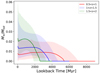 |
Fig. 1. Average distributions of SFHs in HORIZON-AGN. The ribbons show 95% intervals. |
2.3.2. Preparing the photometric training set from the simulation
We computed the galaxy photometry using the technique outlined by Laigle et al. (2019) and Cadiou et al. (2025). This method assumes a Chabrier (2003) initial mass function, single stellar population models from Bruzual & Charlot (2003), and the RV = 3.1 Milky Way dust grain model from Weingartner & Draine (2001). Dust attenuation is modelled along the line of sight of each star particle using the gas-metal mass distribution as a proxy for dust distribution, and it assumes a fixed dust-to-metal mass ratio of 0.3. The photometric flux errors were then added to the fluxes. Specifically, the error was added in a given filter by randomly perturbing the flux. Galaxy flux errors are a combination of a Gaussian error with a standard deviation defined according to the COSMOS2020 depth in a 2″ aperture in each filter, as presented by Weaver et al. (2022), and Poisson noise (using the appropriate instrumental gain). Because of the simulation resolution limit, this simulated sample was limited to galaxies that are more massive than 109 M⊙.
3. Method
3.1. Parameterising SFH
To successfully reconstruct the SFH, it is essential to select an appropriate model that can be effectively inferred. Galaxy SFHs are inherently complex as they encompass a wide range of timescales, from the rapid bursts of star formation seen in starburst galaxies to the slow, steady star formation in more quiescent galaxies. Additionally, galaxies may experience episodic bursts of star formation due to external triggers, such as galaxy-galaxy interactions or mergers. These diverse scenarios give rise to a rich array of SFHs shapes. The challenge arises from the need to distill this complexity into a concise set of parameters that can be effectively learnt and predicted by neural networks, especially when we are interested in recovering the complete posterior distribution and not simply in a maximum likelihood estimate.
Multiple parameterisations have been proposed, from the simplest constant SFR to stochastic processes (e.g. Tacchella et al. 2020; Ciesla et al. 2024; Caplar & Tacchella 2019; Iyer et al. 2019; Wang & Lilly 2020; Wan et al. 2024). Analytical models such as exponentially declining or “delayed” models (e.g. Ciesla et al. 2017) have also been explored extensively (e.g. Ciesla et al. 2018; Carnall et al. 2019).
We used a formalism similar to that in previous works (Iyer et al. 2019; Pacifici et al. 2016b; Behroozi et al. 2019). The SFH was characterised using the total stellar mass M*, with N distinct look-back times corresponding to specific quantiles of M*, and the initial age marking the onset of the SFH. For example, by selecting N = 10, it becomes necessary to determine the initial look-back time t0 marking the start of the SFH, along with times t10, t20, and so on, to t100, which represent the moments when 10%, 20%, and so on, to 100% of the galaxy final stellar mass has been formed, respectively. This latter time should be t = 0 (in look-back time) for galaxies that are still forming stars, but it might be different for completely quenched galaxies (Fig. 3).
Increasing the value of N leads to a more detailed representation of the SFHs (Iyer et al. 2019). However, this improvement is accompanied by an increase in complexity in the estimation process as more details of the SFH need to be inferred. We set N = 30 for a sufficient flexibility without intractability. Fig. 2 illustrates the effect of this approximation. We refer to Appendix C for a more detailed exploration of this trade-off.
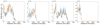 |
Fig. 2. Examples of the effect of our parametrisation on our HORIZON-AGN galaxies. The original SFH binned linearly (blue), and the reconstruction after interpolating between 30 mass quantiles computed directly on the true SFH (orange). |
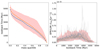 |
Fig. 3. Example of the quantities estimated by our neural network for a randomly selected galaxy in HORIZON-AGN. The true SFH is shown in blue, the estimated mean is plotted in orange, and the 95% confidence interval is shown in red. The mass quantiles estimated by the neural network are shown on the left, and the resulting reconstruction is presented on the right. The SFHs in grey are drawn from the estimated posterior distribution. |
3.2. Simulation-based inference
In our technique, we used simulation-based inference to robustly estimate the SFHs of observed galaxies and provide proper Bayesian uncertainty measurements. This approach combines the power of cosmological simulations with deep learning to bridge the gap between numerical models of galaxy evolution and observed data. An important advantage of cosmological simulations lies in their capacity to create synthetic populations of galaxies, each with a precisely known SFH. These simulations attempt to emulate the complexities of the observable Universe by generating synthetic galaxy catalogues that contain comprehensive details of the SFH for each galaxy. These synthetic galaxies provide a means to directly correlate actual SFHs with the observed photometric data.
A significant advantage of Bayesian inference is its capacity to propagate the uncertainty from prior knowledge and data into parameter estimates. These uncertainties are essential for assessing the reliability of our parameter estimates and provide a quantifiable measure of confidence in the inferred SFHs. The prior represents our initial beliefs or knowledge about the parameter before observing any new data, while the likelihood is a function that describes the probability of the observed data given a particular parameter value.
Simulation-based inference relies on the implicit construction of the likelihood function using samples drawn from a generative model. In the context of our SFH estimation, the likelihood function was constructed by associating the simulated photometry of a galaxy with its SFH.
In practice, SBI uses a deep neural network to parametrise a probability distribution (Cranmer et al. 2020; Papamakarios et al. 2021). This neural network is then optimised to minimise the Kullback-Leibler divergence (Papamakarios et al. 2016) from the true posterior distribution implied by the generative model sampling the training data and the neural network output. This allowed us to construct an estimator of the posterior density directly using a training set of pairs (xi,θi), where xi are the observed quantities (here, the photometry) and θi are the corresponding parameters (here, the formation times). We refer to Papamakarios et al. (2016), Greenberg et al. (2019), and Ho et al. (2024) for more details. We used the SNPE-C (Greenberg et al. 2019) implementation of the sbi package (Tejero-Cantero et al. 2020), using a mask autoregressive flow (Papamakarios et al. 2018) with its default sbi settings as the density estimator. The neural network was trained to estimate p(t0,…,t100|xc) the posterior distribution of the cumulative star formation times t0,…,t100 (see Section 3.1) given a vector of colours xc. The only observed quantities we used for the inference and model checking (see Section 3.3) were the colours corresponding to consecutive bands u*−g,g−r,r−i,i−z,z−Y,Y−J, J−H, and H−Ks. This allowed our estimated SFH to be independent (conditionally on the photometry) of redshift or mass estimates derived from other means. It also provided easy consistency checks on the correlations between mass, redshifts, and formation times (see Figs. 7 and 8) by ensuring that these were not directly fed into the model during training. The observed noise for each galaxy was not used as input either. This relaxed the assumptions on modelling the flux to noise relation and is equivalent to marginalisation over the noise. As demonstrated by Leja et al. (2019), the main factor determining the posterior variance of the SFH is not the photometric noise, but the prior. Moreover, we studied SFHs at the population level and not individual posterior intervals (see Appendix B for an assessment of the effect of photometric noise on our estimates).
In order to standardise the problem, the times t0,…,t100 were rescaled by a constant T such that T>t0 for all galaxies in the training set. T was the same for all galaxies in the sample, and it was slightly higher than the highest value in the training sample. We therefore have
![Mathematical equation: $$ 0 \leq t_i \lt 1 \quad \forall i \in \left [0, 100 \right ], $$](/articles/aa/full_html/2025/07/aa52457-24/aa52457-24-eq1.gif) (1)
(1)
and we rescaled ti after the inference was complete. This restricted the estimated posterior support and allowed a Monte Carlo sampling via the accept-reject algorithm using a uniform distribution over the unit hypercube. As is common with neural network applications for numerical stability (LeCun et al. 1998), the inputs were normalised by removing the mean and dividing by the standard deviation of the colours in the training set.
Figure 4 shows the performance of our estimator on a test set of 10 000 randomly sampled Horizon-AGN that were not used during training. The left panel compares the true times ti associated with the mass quantiles as defined above to the mean of the estimated posterior distributions and shows very good agreement, with a reasonable scatter and no significant bias. The right panel shows the calibration of the credible intervals: for each galaxy in the test set, we estimated the 50%, 68%, and 95% credible intervals and verified whether the true value lay in each interval. A more detailed assessment is presented in Appendix D.2, where we show the error of the formation times of each mass decile. Once again, the estimates were always unbiased, with a scatter σerr≤0.16 dex. We then computed the proportion of intervals that passed this check. For a perfectly calibrated estimator, the 50% (68% and 95%) intervals should contain the true value 50% (68% and 95%) of the time. Our estimator yields well calibrated intervals.
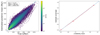 |
Fig. 4. Left: Comparison between the true formation times and the estimated posterior mean in HORIZON-AGN. Perfect inference would lie on the (blue) diagonal line. Our method yields an unbiased estimator with regard to HORIZON-AGN for all timescales. Right: Assessment of the estimated uncertainty calibration with the credibility level on the x-axis, and the realised coverage on the y-axis. For each level (50%, 68%, and 95%), the true value lay in the estimated credibility interval slightly more often than the expected level. A perfect uncertainty calibration would be on the blue diagonal. Our estimator is well calibrated. |
3.3. Prior checking, outlier detection, and data selection
As with every supervised-learning approach, SBI requires that the training data closely match the inference dataset. From a computational perspective, this ensures that the algorithm is optimised on a suitable region of the data space, and from a Bayesian inference perspective, this is equivalent to prior checking (e.g. Gelman et al. 2004; Gelman 2006). More specifically, we needed to ensure that the photometry simulated from HORIZON-AGN was able to adequately model the observed galaxies. When the HORIZON-AGN simulation cannot produce photometry that resembles the observations, we cannot meaningfully perform inference using it in our prior assumptions.
Therefore, we needed a way to confirm for every observed galaxy that the simulation was able to produce galaxies with a photometry similar to the observations. The Bayesian literature refers to these assessments as prior predictive checking or posterior predictive checks (e.g. Gelman et al. 1996). Prior predictive checking consists of simulating mock data from the statistical model by sampling the prior distribution and assessing through a statistical test whether the observation is well covered by the resulting (so-called prior predictive) distribution. When the observation is too far in the tails of the prior predictive distribution for a relevant summary statistic, the model is considered ill-suited to perform inference. Posterior predictive checking describes a similar procedure, but replaces sampling from the prior distribution by sampling from the posterior distribution obtained after fitting the data first. This allowed us to reduce the importance of the prior distribution in the check, but it was too computationally expensive for our case because it requires being able to fit each observation and make new simulations according to this fit for each observed galaxy.
To perform prior predictive checking, we approached it as a problem of outlier detection. The concept of outlier (or anomaly) detection involves establishing a reference distribution and identifying observations that significantly deviate from this norm. By treating the prior predictive distribution as this reference, using outlier detection becomes an effective method for evaluating how well the simulations align with actual observations.
Multiple algorithms spanning the entire machine-learning literature have been proposed to perform outlier detection, from a direct density estimation using parametric methods (e.g. Gaussian mixture models; GMM, McLachlan et al. 2019) or non-parametric approaches (e.g. histogram-based estimators Freedman & Diaconis 1981; Goldstein & Dengel 2012) to deep-learning or kernel-based approaches (e.g. Ting et al. 2020; Ruff et al. 2021). We aggregated several different algorithms to assess whether an observation was accounted for in the simulation.
It is essential to aggregate different outlier detection algorithms to mitigate the biases introduced by the specificity of a given algorithm because it addresses several critical needs in outlier detection and model checking. By combining multiple algorithms, we reduced the risk of relying on a single algorithm that may be prone to producing biased results. This robustness improves the reliability of outlier detection. Different algorithms have different underlying assumptions and approaches for identifying outliers. Aggregating them provides a more comprehensive view of what constitutes an outlier in the data. This diversity of perspectives can help us to capture outliers that may be overlooked by individual algorithms. In practice, we used the pyod Python package (Zhao et al. 2019), which contains the implementation of many outlier detection algorithms. From these, we selected seven that were (see Table 1) well suited to our dataset in terms of dimensionality, number of galaxies, and computational cost. Each algorithm produced a so-called outlier score assessing the compatibility of a given data point with the estimated reference distribution. For example, in the GMM case, we fitted a GMM to the photometric training set. The outlier score for each observed photometry is directly given by the value of the GMM density evaluated at that point. Observations far from the training set will have a low density and, therefore, a low score. By setting a threshold, we categorised which points were deemed outliers according to the scoring of the algorithm. The selection of this threshold is analogous to the construction of a confidence interval; it was set to reject a specified percentage of the reference distribution as outliers.
Algorithms used to detect outliers in order to perform prior checking.
For each algorithm, the score threshold was chosen so as to reject 1% of the simulations as outliers. Each observed galaxy was fed to each of the seven algorithms, and a majority vote among the algorithms dictated whether to reject it or not. A galaxy needed to be classified as an outlier by at least four algorithms to be rejected. This ensured that our detection process was robust to individual algorithmic biases.
3.4. Application of the outlier rejection method to COSMOS2020
We applied the prior checking procedure described above to the COSMOS2020 catalogue. If COSMOS2020 and HORIZON-AGN photometric catalogues followed exactly the same distribution, about 1% of galaxies in COSMOS2020 would be rejected. Remarkably, less than 2% of our catalogue was rejected despite the known differences in the physical parameters between the simulation and the observed galaxies. This means that while physical properties differ, the span of the colour distribution is similar in the simulation and in the observed catalogue. We limited our study to the observed galaxies whose photometric properties were adequately represented in the simulation, regardless of the physical properties. Figure 6 presents the fraction of outliers as a function of SFR, mass, and redshift. The fraction is slightly higher for massive galaxies, especially at high redshift and with very low or very high SFR. This indicates that the colours of these populations are not perfectly reproduced in the HORIZON-AGN simulation. Interestingly, the fraction of outliers stays low for observed galaxies with log M*/M⊙<9, although the simulated sample contains only galaxies with log M*/M⊙>9. This means that the colour distribution of these low-mass galaxies is similar to those of more massive galaxies in the simulated sample, despite their different masses.
4. Results
As illustrated in Fig. 3, when our method considered the median of the posterior distribution, it is ideal for understanding the general build-up of stellar mass in galaxies, but it is less sensitive to short-timescale processes or stochasticity such as multiple close bursts. We caution that the outlier rejection performed in Section 3.4 implies that our analysis sample may be incomplete and potentially biased toward HORIZON-AGN. Fig. 5 illustrates the effect of the various cuts on the mass distribution of star-forming and passive galaxies. This is further discussed in Section 5.2. Nevertheless, we also note that the training was performed on colours instead of fluxes and magnitudes. Therefore, any dependence on the mass of the SFH is a result of the model prediction and not directly derived from the mass-luminosity relation. We therefore also chose not to apply a mass limit, even though the simulated catalogue used in the training was mass limited.
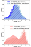 |
Fig. 5. Normalised mass distributions of galaxies in our COSMOS2020 sample. Top: Star-forming galaxies. Bottom: Passive galaxies. The mass distribution of all galaxies in COSMOS (meeting requirements of observed bands, depth, and S/N; see Section 2) is darker and highlights potential biases in our selected sample after outlier rejection (lighter). |
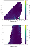 |
Fig. 6. Star formation rate and redshift of galaxies in the COSMOS2020 catalogue that were rejected by our prior predictive check, as a function of their mass. Galaxies that were classified as outliers (see Section 3.3) were excluded from our sample because they are too different in the colour space from the galaxies represented in HORIZON-AGN. |
4.1. Median SFHs of galaxy populations
Fig. 7 shows the median SFH of passive and star-forming galaxies in COSMOS2020 in different mass bins as a function of the look-back time in the redshift ranges 0.5<z<1, 1<z<1.5, 1.5<z<2 and 2<z<2.5 (the number of passive galaxies in the 2.5<z<3 bin was too low to be analysed).
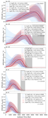 |
Fig. 7. Median SFHs of star-forming (dashed blue lines) and passive (solid red lines) galaxies in COSMOS2020 in several redshift ranges and decomposed into three mass bins, as indicated in the panels. The number of galaxies used to compute the median trend is indicated in the legend. The vertical grey shaded area (whose width depends on the considered redshift range) indicates the maximum look-back time above which the start of the SFH is not compatible with the age of the Universe. |
To determine these trends, we proceeded as follows. For each galaxy, we drew 50 SFHs from the posterior distribution. These were grouped according to mass, photometric redshift, and type (star forming or passive). The figure shows the median and 68% interval of each group. As a reminder, our SFH reconstruction approach did not require galaxy types as input. Types were inferred independently from the rest-frame NUV−r versus r−J diagram (hereafter NUVrJ) colour diagram. For this reason, it is a validation test to confirm that the median SFH for a given galaxy type broadly agreement with expectations. We note from a visual inspection that red galaxies have little to no recent star formation in their reconstructed SFHs, while blue galaxies generally have a much higher recent star formation. Overall, recent star formation is higher in lower-mass galaxies, which is a manifestation of the downsizing phenomena, that is, the fact that massive galaxies have formed most of their mass more rapidly and earlier in the history of the Universe (see e.g. Neistein et al. 2006).
We also note that there is very little evolution of the median SFHs of passive galaxies at all redshifts when they are divided by mass (while the median SFH of star-forming galaxies is strongly mass dependent, as described above). However, for both populations, the 68% intervals are very extended, suggesting a strong diversity of the SFHs within a mass range.
This diversity is expected to manifest itself in the mass-weighted age, the overall slope of the SFH after the peak of star formation, and the smoothness of the SFH (or number of local maxima). These quantities are further examined in Section 4.2.
We next considered the behaviour of the reconstructed SFHs for different galaxies in the NUVrJ diagram. This technique (Ilbert et al. 2013) is now a well-tested method for separating star-forming and passive galaxies using a rest-frame two-colour selection. Fig. 8 shows that the reconstructed SFHs vary smoothly across the NUVrJ diagram from young and highly star-forming galaxies in the bottom left corner (dark blue curve) to passive galaxies at the top (red curve). We observe no abrupt change in SFH between galaxies that lie close to each other in the rest-frame colour space, and the recovered SFH shapes agree with Ilbert et al. (2013). However, the shape of the SFHs of some massive galaxies that were classified as star forming (in the NUVrJ diagram) is questionable (light purple curve), as it seems to fall to zero at the time at which the galaxies are observed. The possible causes for this are discussed in Section 5.1.
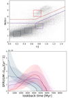 |
Fig. 8. Evolution of the estimated SFHs for galaxies at redshift 0.5<z<1 in COSMOS2020 as a function of their position in the NUVrJ diagram. Top: Four galaxy populations are selected in the star-forming region (blue and clear boxes) and in the passive region (red box). Bottom: Estimated SFHs of galaxies in each box (same colours). |
In addition to showing consistent type-dependent shapes, the reconstructed SFHs are also consistent in terms of galaxy ages. The grey shaded region shows the maximum look-back time beyond which the SFH is incompatible with the age of the Universe. This varies with redshift. For example, at 0.5<z<1, the maximum look-back time of the most massive galaxies is ∼6±0.5 Gyr, which suggests that the time at which the galaxies started to assemble their mass was at most ∼13.8±0.5 Gyr ago, which is consistent with the age of the Universe within the photometric redshift uncertainties. Similarly, in other redshift bins, the times of the first galaxy assembly are compatible with the age of the Universe when we apply the time shift to the maximum look-back time that is deduced from the photometric redshift of the galaxies. This result is particularly remarkable because the galaxy photometric redshifts were not used as input in our reconstruction algorithm.
4.2. Characterisation of individual SFHs and formation redshifts
The nature of processes that shape the star formation and quenching is still unclear and is expected to vary depending on the mass and the environment of the galaxies. For example, quenching could be associated with a cut-off of the gas supply, which would lead to a slow cessation of star formation as the cold gas supply runs out. This cut-off could be driven by tidal effects or stripping processes known as strangulation (Balogh et al. 2000; van den Bosch et al. 2008) in the case of low-mass galaxies in dense environments, or gas heating via shocks (Dekel & Birnboim 2006) or AGN (Dubois et al. 2013) in the case of massive galaxies. Depending on the nature of the process, the quenching timescales could be different. The quenching timescales due to AGN are unclear, as they can also eject strong outflows, which immediately removes the gas from the galaxies and hence turns the star formation off (Springel 2005). Violent events such as disk instabilities or mergers (Snyder et al. 2011) can also temporarily lead to a very rapid exhaustion of the gas reservoir via an intense burst of star formation, but they in turn rapidly quench the galaxy afterward. For galaxies in the hot intracluster medium, gas can be quickly removed via ram-pressure stripping (Abadi et al. 1999), which finally halts star formation on a short timescale (see also Park et al. 2022).
Although this list is not exhaustive, we emphasise that given their different timescales, these processes have different impacts on the shape of the SFH. Therefore, it is essential to derive relevant summary statistics to identify the characteristic patterns and their variation with mass and redshift.
From each SFH, we measured the following summary statistics, described below: the slope, the formation epoch (i.e. the age of the Universe when the galaxy was at its mean age) tU,form, and redshift zU,form, the number of maxima m, and the time of the first peak.
4.2.1. Mass-weighted formation age, ageform
For each galaxy, the mass-weighted formation age, ageform, is defined as
 (2)
(2)
where tfirst is the look-back age corresponding to the start of the SFH, and t = 0 corresponds to the observation. ageform is in units of look-back time. In practice, it is almost equivalent to the look-back age at which the galaxy formed half of its stellar mass t50. Using ageform and the photometric redshift in COSMOS2020 or the exact galaxy redshift in HORIZON-AGN, we then defined tU,form, which is the age of the Universe when the galaxy was at ageform, and the corresponding redshift zU,form.
4.2.2. Slope
The slope estimates the overall trend of the SFH since the formation age ageform, and it is defined as
![Mathematical equation: $$ {\mathrm {slope}} \left [{\mathrm {dex}}\right ] = \frac {\log {\mathrm {SFR}}_{95} - \log {\mathrm {SFR}}_{{\mathrm {form}}}}{t_{95}-{\mathrm {age}}_{\mathrm {form}}} \times t_H(z), $$](/articles/aa/full_html/2025/07/aa52457-24/aa52457-24-eq3.gif) (3)
(3)
where SFR95 is the SFR at the time t95 at which the galaxy formed 95% of its mass, SFRform is the SFR at the time ageform, and tH(z) is the Hubble time at z. The slope is measured on a smoothed SFH, where the SFH is smoothed with a Gaussian kernel with a standard deviation of 100 Myr, as shown in Fig. 9 (compare the thin and thick purple and cyan lines in the left panel). We chose t95 because it is the last estimated time by our algorithm before t100, and this avoids undefined slope values when SFR100 = 0, whereas SFR95 = 0 is less likely because of the smoothing. A positive slope indicates that the galaxy forms overall fewer stars now than it formed at ageform.
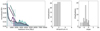 |
Fig. 9. Illustration of our method for measuring the formation age ageform, slope, number of maxima, and age of the first peak for an individual SFH drawn from the posterior distribution of each galaxy. The left panel shows two realisations of the SFH for the same galaxy from the COSMOS2020 catalogue (purple and cyan lines, smoothed with a Gaussian kernel with a standard deviation 100 Myr), together with the median over 50 realisations (grey line). The dashed vertical line indicates ageform, which was then used to compute the slope (solid straight segments). The circles indicate the position of the persistent maxima. The middle and right panels show the histograms of the numbers of maxima and slopes over 50 realisations. |
4.2.3. Number of maxima and age of the first peak
We also estimated the number of maxima m. Local maxima were identified and were filtered to keep only the highly persistent maxima4. The persistence of a peak simply quantifies the longevity of this peak as an isolated component in an excursion set (the set of values greater than a threshold) that evolves with a decreasing threshold (see e.g. Edelsbrunner & Letscher 2002). The most persistent peaks are therefore the most prominent peaks in the normalised SFH. The number of maxima is therefore dependent on the chosen persistence threshold, which should be chosen in the same unit as the SFH. Because all SFHs sum to 1, galaxies that formed a long time ago have overall lower SFH values than those that formed recently. Therefore, we chose a persistence threshold of the same order of magnitude as the standard deviation of different realisations at a given timestep (each realisation was normalised by the number of non-null values in each SFH). We caution that this extraction of maxima was performed on the normalised SFH. Therefore, the absolute mass formed under an SFH peak at a given persistence in high-mass galaxies is higher than in low-mass galaxies. However, the fraction of the mass that formed would be comparable. In this sense, the number of maxima allowed us to quantify the smoothness of the SFH.
We note that varying this persistence threshold around this value does not change the relative trend within the galaxy populations, but simply shifts it up or down. Finally, we also estimated the age of the Universe at the first peak of the mass assembly tfirst peak.
For each galaxy, these quantities were estimated on 50 individual realisations of the SFH from the posterior and were then averaged. Figure 9 illustrates the method of measuring these quantities in two individual realisations. The quality of these estimators is studied in Appendix D, where we rely on the comparison between the measurement of the true SFH in HORIZON-AGN and their reconstructed version.
4.3. The diversity of SFH slopes as a function of mass
Figure 10 shows the slopes of the reconstructed SFH as a function of stellar mass for the full population (top) and the quiescent population (bottom, identified from the NUVrJ diagram) in COSMOS2020 and HORIZON-AGN, respectively. The same S/N cut was applied to HORIZON-AGN and COSMOS2020. The error bars indicate the standard deviation around the mean. The redshift ranges were chosen to encompass similar comoving volumes in COSMOS, in order to mitigate the possible effect of cosmic variance when one redshift bin is compared to another. We note, however, that the intrinsic 100 Mpc/h size of the native HORIZON-AGN box from which the light cone was extracted implies a cosmic variance at the 100 Mpc/h scale for HORIZON-AGN. The slopes were estimated based on 50 realisations drawn from the posterior distribution and were then averaged.
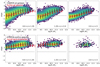 |
Fig. 10. Slope of the reconstructed SFH, as defined in Equation (3) in COSMOS2020 (solid black lines with error bars) and HORIZON-AGN (dashed red lines) for all galaxies in the sample (top) and passive only (bottom). For each galaxy, individual slopes computed from 50 SFHs drawn from the posterior distribution were averaged. The two first redshift ranges were chosen to encompass similar comoving volumes in order to mitigate possible cosmic variance effects in the galaxy distribution. The hexagons are colour-coded by the logarithm of the galaxy number density in COSMOS2020 in the considered redshift bin. |
There is a large dispersion of slopes at a given mass, which is consistent with the extended 68% interval in Fig. 7. In addition, there is a clear dependence on mass for the entire population, and this dependence is stronger in COSMOS2020 than in HORIZON-AGN. As expected, the slope is larger for higher-mass galaxies, indicating that they formed most of their mass closer to the formation age ageform and are more likely to have quenched by the time they are observed. On the other hand, low-mass galaxies have a negative or very small slope. We note that the low- to high-mass transition is more pronounced in COSMOS2020 than in HORIZON-AGN. In particular, observed galaxies form stars more vigorously than in simulations, with negative slopes (indicating rising SFHs) up to log M*/M⊙<10.5. This behaviour was previously highlighted by Kaviraj et al. (2017), who found that the low-mass end of the star-forming main sequence formed stars less vigorously in HORIZON-AGN.
We find that massive galaxies generally have larger positive slopes in COSMOS2020 than in HORIZON-AGN. This might indicate a more drastic quenching. This agrees with Dubois et al. (2016), who showed that massive simulated galaxies generally contain larger residual star formation than in observations. Because we normalised the slope by the Hubble time tH(z), there is no redshift dependence of the median slope in COSMOS2020 at a given mass, but we find a larger dispersion at lower redshift.
For passive galaxies, the slope weakly depends on stellar mass in the two lowest-redshift bins in COSMOS2020, and the SFHs of more massive galaxies drop slightly more rapidly since their formation age than lower-mass galaxies. This trend is also consistent with Fig. 7. This behaviour is not seen in HORIZON-AGN or in higher-redshift bins. However, at a given stellar mass, we also note the large diversity of possible slopes, especially at low redshift. This might indicate distinct quenching mechanisms.
A refinement of the analysis of the slope as a function of other quantities, such as the environment or the halo mass, would be a promising avenue for understanding the quenching mechanisms of passive galaxies, but is beyond the scope of this study.
4.3.1. Number of maxima
Figure 11 shows the number of maxima in the reconstructed normalised SFHs as a function of the formation age ageform and the stellar mass in COSMOS2020 (top) and HORIZON-AGN (bottom). The number of maxima was computed on 50 individual realisations from the posterior distribution and averaged per galaxy, as described in Section 4.2.3 and Fig. 9.
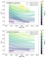 |
Fig. 11. Number of maxima 〈m〉 in the COSMOS (top) and Horizon-AGN (bottom) SFHs as a function of stellar mass, colour-coded by the formation look-back time for two different redshift bins. The number of maxima is computed as described in Section 4.2.3 and Fig. 9. |
We find that the number of maxima depends on the stellar mass and on the formation age. At a given mass, galaxies that formed the bulk of their mass a longer time ago are more likely to have experienced a second and possibly third peak of star formation. This trend is found at all masses and in COSMOS2020 and HORIZON-AGN. Furthermore, high-mass galaxies have fewer local maxima in their normalised SFHs than the least massive galaxies, suggesting that they assembled most of their mass at once, and the fraction of mass that could form in subsequent episodes is much lower (i.e. these late peaks do not meet our persistence criterion for the peak identification). The trend is more pronounced in COSMOS2020 than in HORIZON-AGN. The phenomenon can also be interpreted as the accumulation of several disconnected star formation bursts in massive galaxies, which might result in a general smoothing effect (see also Iyer et al. 2019, for a similar interpretation based on the central limit theorem).
With a different method for identifying peaks, Iyer et al. (2019) also found a mass dependence of the number of peaks in the SFH especially at low redshift (z∼0.5), with a higher probability for low-mass galaxies (log M*/M⊙<10.5) to exhibit several peaks than high-mass galaxies. This agrees with our findings. The trend they found is less clear at higher redshifts and possibly reverses, but we note that galaxies were not divided by ageform in their analysis. Finally, we emphasise that the mass dependence of the number of maxima in the SFH is particularly interesting considering that the mass was not an input of the reconstruction, since the algorithm is designed to infer SFHs from colours.
Comparing the results in two different redshift bins, we note that at a fixed stellar mass and formation age, the average number of maxima is smaller at higher than at lower redshift, especially for low-mass galaxies with a young look-back formation age. This suggests that the growth of galaxies at a lower redshift is less smooth than at higher redshift.
4.3.2. Formation redshift
Finally, we measured the formation epoch tU,form (the age of the Universe at the mass-weighted age of the galaxy) of all galaxies in the sample. To provide a direct comparison with existing observations, we first restricted our analysis to 0.9<z<1.4 because data from the literature are mostly confined to this redshift range. In particular, Fig. 12 shows the formation epoch (the age of the Universe at which the galaxy age was equal to its mass-weighted age) as a function of stellar mass for all galaxies (left) and passive galaxies (middle), as well as the age of the Universe at the first peak for passive galaxies (right). At a given stellar mass, the galaxies exhibit a wide variety of formation epochs. Low-mass galaxies have formed the bulk of their mass after more massive galaxies.
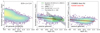 |
Fig. 12. Formation epoch tU,form (i.e. the age of the Universe corresponding to the mass-weighted age of the galaxy as defined in Equation (2)) vs. mass in COSMOS2020 at 0.9<z<1.4 compared to the literature for all galaxies (left) and passive galaxies alone (middle). The right panel displays the age of the Universe corresponding to the first peak in the SFH. The black line shows the best-fit for the passive galaxies in COSMOS2020, and the red line shows the best-fit in HORIZON-AGN. |
We compared the formation epochs of passive galaxies with data from Kaushal et al. (2024) at 0.6<z<1 in the LEGA-C sample (using their reconstruction based on the code Prospector described by Johnson et al. 2021; see also our comparison in Appendix A.1), data from the TNG100 (Pillepich et al. 2018) and SIMBA (Davé et al. 2019) simulations5, and the relation fitted by Carnall et al. (2019) at 1<z<1.3 and Tacchella et al. (2022b) at z∼0.8. The estimated formation epochs of passive galaxies in COSMOS2020 and HORIZON-AGN is very similar to those reported by Kaushal et al. (2024) and span the same range as those reported by Carnall et al. (2019) and Tacchella et al. (2022b), but with little variation with mass. We note, however, that due to the sparsity of their sample, the slope of the relation fitted in these papers for galaxies log M*/M⊙>10.5 might be very sensitive to the inclusion or exclusion of the highest-mass galaxies (log M*/M⊙>11.5), where the galaxy density is also lowest. On the other hand, our outlier rejection algorithm tends to reject the most massive galaxies (see Fig. 6), and therefore, our sample could be incomplete at the high-mass end, which would bias the slope of this fit.
Following Gallazzi et al. (2014) at z∼0.7 and Carnall et al. (2019) at 1<z<1.3, we also fitted the relation between the formation epochs tU,form and the stellar mass. We performed this fit at 0.9<z<1.4 to provide a direct comparison with existing observational data, and we found for the passive populations
 (4)
(4)
We also fitted the relation between the age of the Universe at the first peak t1st peak and the stellar mass, which provided an even flatter relation,
 (5)
(5)
In an effort to further understand the build-up of the population of passive galaxies, Fig. 13 shows the formation epoch (the age of the Universe at which the galaxy age was equal to its mass-weighted age) and age of the Universe at the first peak as a function of the age of the Universe tUniverse at which the galaxies were observed for all passive galaxies in COSMOS2020 (left and middle panels, respectively). We show only galaxies that are more massive than log M*/M⊙>8.6 to guarantee completeness up to z∼1.5 (see e.g. Shuntov et al. 2022). At an age of the Universe older than 5 Gyr (z<1.3), the passive population lacks galaxies with formation epochs below ∼2 Gyr (formation redshift above zU,form>3.3), whereas galaxies with this formation epoch were found at higher redshift. This might be due to incompleteness in our sample as a result of the outlier rejection algorithm. It is also possible that these passive galaxies have rejuvenated and therefore moved to the star-forming population by z∼1.3, or that they experienced a recent peak of mass assembly, which shifted their formation epoch towards more recent epochs.
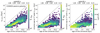 |
Fig. 13. Formation epoch tU,form (left) and age of the Universe at the first peak (middle and right) as a function of the redshift at which the galaxies are observed (or the corresponding age of the Universe) for passive galaxies in COSMOS2020. The hexagons are colour-coded by density (left and middle) or stellar mass (right). |
In the middle panel, the position of the first peak only weakly depends on the redshift. However, the mean mass of the population at a given  decreases, indicating the appearance of a new population of lower-mass galaxies. These galaxies would have formed almost as early as the first massive passive galaxies because the position of the first peak does not change drastically. However, they might have experienced star formation for a longer period of time or in multiple bursts, in which case they would join the passive population later. Overall, these passive galaxies have experienced major episodes of mass assembly by z∼3 (1<tUniverse/Gyr<4, i.e. 2.2<z<5.8), regardless of their mass. Finally, we note that from tUniverse∼7.5 Gyr (z∼0.7), the scatter of t1st peak increases when very low-mass galaxies (log M*/M⊙<9) that formed recently are included; these might be satellite galaxies (see also Weaver et al. 2023, about the build-up of the passive population in COSMOS2020). These recently formed low-mass galaxies do not seem to represent an important fraction of the passive population at higher redshift (z>0.7), but it is still possible that low-mass passive galaxies are missing from our sample at higher redshift because we rejected outliers (see Fig. 5).
5. Caveats and perspectives
5.1. Sensitivity to filter selection
Section 4 showed that our algorithm generally performed as expected (as confirmed by the comparison with the literature in Appendix A.1). However, as for all SED fitting, the performances can vary and degeneracies can appear depending on the chosen set of colors. For instance, we found a tendency for our network to inaccurately classify some massive dusty star-forming galaxies as passive. This tendency was amplified when we removed the H-band. This is shown in Fig. 14, which shows the distribution of our 0.5<z<1 sample in the NUVrJ diagram.
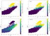 |
Fig. 14. NUVrJ diagrams showing the separation of active and passive galaxies in 0.5<z<1 in COSMOS2020. The dashed line is from Ilbert et al. (2013). Top left: Fraction of passive galaxies (colours) selected as those with a LePHARE estimate of log(sSFR/yr−1)<−11. Top right: Same fraction from sSFRs estimated by our SBI method using all filters. Bottom left: Distribution of dust, as estimated by LePHARE. Bottom right: Same fraction from sSFRs estimated by our SBI method, but without the H Band. The SFH inferred by SBI without the H band on the right side of the panel corresponds to more passive galaxies than estimated with an SED fitting, which identifies these galaxies as active, but dusty. |
The upper and middle panels illustrate an inconsistency between our SFHs and the LePHARE SFR estimates. According to Ilbert et al. (2013) and as illustrated in the top panel, passive galaxies with a specific SFR (sSFR) of log(sSFR/yr−1)<−11 should lie above the red line in the NUVrJ diagram. However, when the H band was removed, our method found some galaxies below the line with a passive SFH. Since this part of the diagram is populated by massive dusty galaxies (compared to the bottom panel), our estimator might be confusing red dust-attenuated galaxies with passive galaxies. We note that the perfect separation in the top panel is somewhat artificial: We used rest-frame magnitudes computed by LePHARE, and therefore, we expect that independent sSFR estimates do not match this pattern exactly.
5.2. Validity of our HORIZON-AGN prior
Our simulated SFHs are only representative of real SFHs when all internal (e.g., feedback and morphology) and external processes (interaction, mergers, and matter acquisition from the cosmic web) that shape them are correctly accounted for in the simulation. Each effect is expected to act in a given epoch on a particular scale and at a particular timescale and will imprint a specific signature on the galaxy SFH and spectra. Our network was trained on the HORIZON-AGN simulation, and therefore, the SFHs that we can predict are those of the HORIZON-AGN galaxies. However, we know that HORIZON-AGN does not predict the correct abundances of the passive galaxy population and overestimates the stellar-to-halo mass relation(see Section 2.3). Some SFHs might therefore be missing in the simulations, which might affect the prediction in observations. This effect is mitigated to some extent by the fact that observed galaxies with colours that are very different from the simulated colours are rejected through the outlier-detection method: We do not pretend to reconstruct the SFH of a galaxy when its photometry does not appear in the simulation. Nevertheless, this limitation is inherent to any SED-fitting code: The prior distributions over SFHs are always of primordial importance even though there is no obvious guideline for prior elicitation (see e.g. Leja et al. 2019). We emphasise that our method enforces a prior that is well motivated by hydrodynamical simulations at a lower computational cost than classical SED-fitting techniques. The analysis shown in Fig. 10 is reassuring. The trend of the SFH slope as a function of mass is different for COSMOS2020 and HORIZON-AGN, which suggests that the result of the reconstruction is not entirely determined by the prior.
Furthermore, it is important to note that we rejected observed galaxies whose photometry is incompatible with the simulations by design (Section 3.4). The predictive power of our network is therefore limited to galaxies whose photometry is similar to that the HORIZON-AGN simulation, and the analysis of the sample of passive galaxies might be partially incomplete (see e.g. the discussion of Fig. 13 in Section 4.3.2). A possible improvement of our method would be to enrich the training set with photometry derived from other hydrodynamical cosmological simulations or from semi-analytical models.
5.3. Distinguishing in situ and ex situ mass assembly
One particularity of our method is that we reconstructed the history of the star formation instead of the history of the mass assembly. Therefore, we cannot distinguish in situ and ex situ stellar populations (see e.g. Kaushal et al. 2024, for a discussion). For galaxies that underwent mergers, we reconstructed the cumulative SFHs of the different progenitors that are part of the final passive galaxies. One possible improvement would be to simultaneously learn the merger and star-formation histories of the galaxies with our SBI method from their photometry.
6. Conclusion
We presented a novel method for performing a Bayesian estimation of the SFH of galaxies from photometry using simulation-based inference with HORIZON-AGN hydrodynamical simulations together with a suitable parametrisation of the SFH. We showed that the method was able to correctly reconstruct the entire SFH of galaxies based on simulations. We applied it to the COSMOS2020 catalogue. Our results are listed below.
-
Based on simulated data, SBI was able to properly estimate the entire SFH and to accurately quantify the Bayesian uncertainties (Fig. 4).
-
The shapes of our SFHs broadly agree with the NUVrJ diagram classification of passive galaxies (Figs. 7 and 8). In addition, the estimates of the time of the first star formation of galaxies agree with age of the Universe at the corresponding redshift, even though we did not use any information but the colours as input. Although the mass was not used as input, the median SFHs of the star-forming galaxies show a wide diversity on average that depends on the mass and redshift, while the median SFHs of passive galaxies have very limited range of histories, with almost no dependence on the mass.
-
We extracted summary statistics (the slope, the number of maxima, and the formation age) from the SFH of individual galaxies (Fig. 9). The slopes of the SFHs of passive galaxies showed only a weak trend with stellar mass at z<1.35, but had a significant scatter. This indicates that parameters other than the mass might drive quenching. On the other hand, star-forming galaxies showed a clear mass dependence, with lower-mass galaxies undergoing more vigorous recent star formation. Overall, the galaxy slopes in COSMOS2020 varied over a wider range than in HORIZON-AGN (Fig. 10).
-
Low-mass galaxies exhibit more peaks in their mass assembly history than high-mass galaxies, and the trend is more evident in COSMOS2020 than in HORIZON-AGN (Fig. 11).
-
At a given mass, we found a large diversity of formation redshifts, the dependence of the formation redshift on mass is weak for passive galaxies (Fig. 12). Most passive galaxies with log M*/M⊙>9 had a first event of mass assembly at about z∼3 (2.2<z<5.8), regardless of their mass. From z∼0.7, some log M*/M⊙<9 that formed more recently joined the passive population (Fig. 13).
Acknowledgments
CL thanks the Programme National Galaxies and Cosmologie (PNCG) for funding. GA acknowledges funding support from the Initiative Physique des Infinis (IPI), a research training program of the Idex SUPER at Sorbonne Université. The authors acknowledge the support of the French Agence Nationale de la Recherche (ANR), under grant ANR-22-CE31-0007 (project IMAGE). This project has received financial support from CNRS and CNES through the MITI interdisciplinary programs. This work was made possible by utilising the CANDIDE cluster at the Institut d’Astrophysique de Paris. The cluster was funded through grants from the PNCG, CNES, DIM-ACAV, the Euclid Consortium, and the Danish National Research Foundation Cosmic Dawn Center (DNRF140). It is maintained by Stephane Rouberol. LC acknowledges support from the French government under the France 2030 investment plan, as part of the Initiative d’Excellence d’Aix-Marseille Université - A*MIDEX AMX-22-RE-AB-101.
Using the COSMOS2020 FLAG_COMBINED column.
In HORIZON-AGN, most of the stellar mass losses occur on a relatively short timescale (∼100 Myr; see e.g. Figure A5 in Laigle et al. 2019), so the difference between the simulated SFH with or without correction for the stellar mass losses will mostly concern the amount of mass in our last SFH bin, and it might change it by ∼10%.
We used this freely distributed implementation: https://www.csc.kth.se/∼weinkauf/notes/persistence1d.html
Datapoints were extracted from Kaushal et al. (2024) with https://plotdigitizer.com/app
We note that if studying those specific galaxies was our goal, we would only need to tune the training set of our network to account for the missing bands.
References
- Abadi, M. G., Moore, B., & Bower, R. G. 1999, MNRAS, 308, 947 [Google Scholar]
- Aggarwal, C. C. 2016, Outlier Analysis, 2nd edn. (Springer Publishing Company, Incorporated) [Google Scholar]
- Arnouts, S., Moscardini, L., Vanzella, E., et al. 2002, MNRAS, 329, 355 [Google Scholar]
- Aubert, D., Pichon, C., & Colombi, S. 2004, MNRAS, 352, 376 [Google Scholar]
- Aufort, G., Ciesla, L., Pudlo, P., & Buat, V. 2020, A&A, 635, A136 [NASA ADS] [CrossRef] [EDP Sciences] [Google Scholar]
- Balogh, M. L., Navarro, J. F., & Morris, S. L. 2000, ApJ, 540, 113 [Google Scholar]
- Behroozi, P., Wechsler, R. H., Hearin, A. P., & Conroy, C. 2019, MNRAS, 488, 3143 [NASA ADS] [CrossRef] [Google Scholar]
- Bertin, E., & Arnouts, S. 1996, A&AS, 117, 393 [NASA ADS] [CrossRef] [EDP Sciences] [Google Scholar]
- Boquien, M., Burgarella, D., Roehlly, Y., et al. 2019, A&A, 622, A103 [NASA ADS] [CrossRef] [EDP Sciences] [Google Scholar]
- Brammer, G. B., van Dokkum, P. G., & Coppi, P. 2008, ApJ, 686, 1503 [Google Scholar]
- Breunig, M. M., Kriegel, H. P., Ng, R. T., & Sander, J. 2000, in Proceedings of the 2000 ACM SIGMOD International Conference on Management of Data, SIGMOD ’00 (New York, NY, USA: Association for Computing Machinery), 93 [Google Scholar]
- Bruzual, G., & Charlot, S. 2003, MNRAS, 344, 1000 [NASA ADS] [CrossRef] [Google Scholar]
- Cadiou, C., Laigle, C., & Agertz, O. 2025, MNRAS, 537, 1869 [Google Scholar]
- Caplar, N., & Tacchella, S. 2019, MNRAS, 487, 3845 [NASA ADS] [CrossRef] [Google Scholar]
- Carnall, A. C., Leja, J., Johnson, B. D., et al. 2019, ApJ, 873, 44 [Google Scholar]
- Chabrier, G. 2003, PASP, 115, 763 [Google Scholar]
- Ciesla, L., Elbaz, D., & Fensch, J. 2017, A&A, 608, A41 [NASA ADS] [CrossRef] [EDP Sciences] [Google Scholar]
- Ciesla, L., Elbaz, D., Schreiber, C., Daddi, E., & Wang, T. 2018, A&A, 615, A61 [NASA ADS] [CrossRef] [EDP Sciences] [Google Scholar]
- Ciesla, L., Elbaz, D., Ilbert, O., et al. 2024, A&A, 686, A128 [NASA ADS] [CrossRef] [EDP Sciences] [Google Scholar]
- Cranmer, K., Brehmer, J., & Louppe, G. 2020, Proc. Natl. Acad. Sci., 117, 30055 [Google Scholar]
- Davé, R., Anglés-Alcázar, D., Narayanan, D., et al. 2019, MNRAS, 486, 2827 [Google Scholar]
- Dekel, A., & Birnboim, Y. 2006, MNRAS, 368, 2 [NASA ADS] [CrossRef] [Google Scholar]
- Dubois, Y., Gavazzi, R., Peirani, S., & Silk, J. 2013, MNRAS, 433, 3297 [CrossRef] [Google Scholar]
- Dubois, Y., Pichon, C., Welker, C., et al. 2014, MNRAS, 444, 1453 [Google Scholar]
- Dubois, Y., Peirani, S., Pichon, C., et al. 2016, MNRAS, 463, 3948 [Google Scholar]
- Edelsbrunner, H., Letscher, D., & Zomorodian 2002, Discret. Comput. Geom., 28, 511 [Google Scholar]
- Euclid Collaboration (Scaramella, R., et al.) 2022a, A&A, 662, A112 [NASA ADS] [CrossRef] [EDP Sciences] [Google Scholar]
- Euclid Collaboration (Moneti, A., et al.) 2022b, A&A, 658, A126 [NASA ADS] [CrossRef] [EDP Sciences] [Google Scholar]
- Euclid Collaboration (Mellier, Y., et al.) 2025a, A&A, 697, A1 [Google Scholar]
- Euclid Collaboration (McPartland, C. J. R., et al.) 2025b, A&A, 695, A259 [Google Scholar]
- Freedman, D., & Diaconis, P. 1981, Z. Wahrsch. Verw. Geb., 57, 453 [Google Scholar]
- Gallazzi, A., Bell, E. F., Zibetti, S., Brinchmann, J., & Kelson, D. D. 2014, ApJ, 788, 72 [Google Scholar]
- Gelman, A. 2006, Bayesian Anal., 1, 515 [Google Scholar]
- Gelman, A., Meng, X. -L., & Stern, H. 1996, Stat. Sin., 6, 733 [Google Scholar]
- Gelman, A., Carlin, J. B., Stern, H. S., & Rubin, D. B. 2004, Bayesian Data Analysis, 2nd edn. (Chapman and Hall/CRC) [Google Scholar]
- Goldstein, M., & Dengel, A. 2012, Histogram-based Outlier Score (HBOS): A fast Unsupervised Anomaly Detection Algorithm [Google Scholar]
- Gould, K. M. L., Brammer, G., Valentino, F., et al. 2023, AJ, 165, 248 [NASA ADS] [CrossRef] [Google Scholar]
- Greenberg, D. S., Nonnenmacher, M., & Macke, J. H. 2019, arXiv e-prints [arXiv:1905.07488] [Google Scholar]
- Hardin, J., & Rocke, D. M. 2004, Comput. Stat. Data Anal., 44, 625 [Google Scholar]
- Heavens, A. F., Jimenez, R., & Lahav, O. 2000, MNRAS, 317, 965 [NASA ADS] [CrossRef] [Google Scholar]
- Ho, M., Bartlett, D. J., Chartier, N., et al. 2024, Open J. Astrophys., 7, 54 [NASA ADS] [CrossRef] [Google Scholar]
- Ilbert, O., Tresse, L., Zucca, E., et al. 2005, A&A, 439, 863 [NASA ADS] [CrossRef] [EDP Sciences] [Google Scholar]
- Ilbert, O., Arnouts, S., McCracken, H. J., et al. 2006, A&A, 457, 841 [NASA ADS] [CrossRef] [EDP Sciences] [Google Scholar]
- Ilbert, O., McCracken, H. J., Le Fèvre, O., et al. 2013, A&A, 556, A55 [NASA ADS] [CrossRef] [EDP Sciences] [Google Scholar]
- Iyer, K. G., Gawiser, E., Faber, S. M., et al. 2019, ApJ, 879, 116 [NASA ADS] [CrossRef] [Google Scholar]
- Johnson, B., & Leja, J. 2017, https://doi.org/10.5281/zenodo.1116491 [Google Scholar]
- Johnson, B. D., Leja, J., Conroy, C., & Speagle, J. S. 2021, ApJS, 254, 22 [NASA ADS] [CrossRef] [Google Scholar]
- Kaushal, Y., Nersesian, A., Bezanson, R., et al. 2024, ApJ, 961, 118 [NASA ADS] [CrossRef] [Google Scholar]
- Kaviraj, S., Laigle, C., Kimm, T., et al. 2017, MNRAS, 467, 4739 [NASA ADS] [Google Scholar]
- Komatsu, E., et al. 2011, ApJS, 192, 18 [NASA ADS] [CrossRef] [Google Scholar]
- Laigle, C., Davidzon, I., Ilbert, O., et al. 2019, MNRAS, 486, 5104 [Google Scholar]
- Laureijs, R., Amiaux, J., Arduini, S., et al. 2011, arXiv e-prints [arXiv:1110.3193] [Google Scholar]
- LeCun, Y., Bottou, L., Bengio, Y., & Haffner, P. 1998, in Gradient-based learning applied to document recognition, Proceedings of the IEEE, 86, 2278 [CrossRef] [Google Scholar]
- Leja, J., Carnall, A. C., Johnson, B. D., Conroy, C., & Speagle, J. S. 2019, ApJ, 876, 3 [Google Scholar]
- Leja, J., Speagle, J. S., Ting, Y. -S., et al. 2022, ApJ, 936, 165 [NASA ADS] [CrossRef] [Google Scholar]
- Lower, S., Narayanan, D., Leja, J., et al. 2020, ApJ, 904, 33 [NASA ADS] [CrossRef] [Google Scholar]
- Madau, P., & Dickinson, M. 2014, ARA&A, 52, 415 [Google Scholar]
- McCracken, H. J., Milvang-Jensen, B., Dunlop, J., et al. 2012, A&A, 544, A156 [NASA ADS] [CrossRef] [EDP Sciences] [Google Scholar]
- McLachlan, G. J., Lee, S. X., & Rathnayake, S. I. 2019, Annu. Rev. Stat. Appl., 6, 355 [Google Scholar]
- Neistein, E., van den Bosch, F. C., & Dekel, A. 2006, MNRAS, 372, 933 [NASA ADS] [CrossRef] [Google Scholar]
- Oke, J. B., & Gunn, J. E. 1983, ApJ, 266, 713 [NASA ADS] [CrossRef] [Google Scholar]
- Pacifici, C., Kassin, S. A., Weiner, B. J., et al. 2016a, ApJ, 832, 79 [Google Scholar]
- Pacifici, C., Oh, S., Oh, K., Lee, J., & Yi, S. K. 2016b, ApJ, 824, 45 [NASA ADS] [CrossRef] [Google Scholar]
- Papamakarios, G., & Murray, I. 2016, in Advances in Neural Information Processing Systems, eds. D. Lee, M. Sugiyama, U. Luxburg, I. Guyon, & R. Garnett (Curran Associates, Inc.), 29 [Google Scholar]
- Papamakarios, G., Pavlakou, T., & Murray, I. 2018, arXiv e-prints [arXiv:1705.07057] [Google Scholar]
- Papamakarios, G., Nalisnick, E., Rezende, D. J., Mohamed, S., & Lakshminarayanan, B. 2021, J. Mach. Learn. Res., 22, 1 [Google Scholar]
- Park, M., Tacchella, S., Nelson, E. J., et al. 2022, MNRAS, 515, 213 [NASA ADS] [CrossRef] [Google Scholar]
- Park, M., Belli, S., Conroy, C., et al. 2024, ApJ, 976, 72 [Google Scholar]
- Peng, Y. -J., Lilly, S. J., Kovač, K., et al. 2010, ApJ, 721, 193 [NASA ADS] [CrossRef] [Google Scholar]
- Picouet, V., Arnouts, S., Le Floc’h, E., et al. 2023, A&A, 675, A164 [NASA ADS] [CrossRef] [EDP Sciences] [Google Scholar]
- Pillepich, A., Springel, V., Nelson, D., et al. 2018, MNRAS, 473, 4077 [Google Scholar]
- Planck Collaboration XVI. 2014, A&A, 571, A16 [NASA ADS] [CrossRef] [EDP Sciences] [Google Scholar]
- Ramaswamy, S., Rastogi, R., & Shim, K. 2000, SIGMOD Rec., 29, 427 [Google Scholar]
- Ruff, L., Kauffmann, J. R., Vandermeulen, R. A., et al. 2021, Proc. IEEE, 109, 756 [Google Scholar]
- Santini, P., Castellano, M., Fontana, A., et al. 2022, ApJ, 940, 135 [NASA ADS] [CrossRef] [Google Scholar]
- Sawicki, M., Arnouts, S., Huang, J., et al. 2019, MNRAS, 489, 5202 [NASA ADS] [Google Scholar]
- Scoville, N., Aussel, H., Brusa, M., et al. 2007, ApJS, 172, 1 [Google Scholar]
- Shuntov, M., McCracken, H. J., Gavazzi, R., et al. 2022, A&A, 664, A61 [NASA ADS] [CrossRef] [EDP Sciences] [Google Scholar]
- Snyder, G. F., Cox, T. J., Hayward, C. C., Hernquist, L., & Jonsson, P. 2011, ApJ, 741, 77 [NASA ADS] [CrossRef] [Google Scholar]
- Spacek, A., Richardson, M. L. A., Scannapieco, E., et al. 2018, ApJ, 865, 109 [NASA ADS] [CrossRef] [Google Scholar]
- Springel, V. 2005, MNRAS, 364, 1105 [Google Scholar]
- Suess, K. A., Leja, J., Johnson, B. D., et al. 2022, ApJ, 935, 146 [NASA ADS] [CrossRef] [Google Scholar]
- Tacchella, S., Forbes, J. C., & Caplar, N. 2020, MNRAS, 497, 698 [Google Scholar]
- Tacchella, S., Finkelstein, S. L., Bagley, M., et al. 2022a, ApJ, 927, 170 [NASA ADS] [CrossRef] [Google Scholar]
- Tacchella, S., Conroy, C., Faber, S. M., et al. 2022b, ApJ, 926, 134 [NASA ADS] [CrossRef] [Google Scholar]
- Tejero-Cantero, A., Boelts, J., Deistler, M., et al. 2020, J. Open Source Softw., 5, 2505 [NASA ADS] [CrossRef] [Google Scholar]
- Teyssier, R. 2002, A&A, 385, 337 [CrossRef] [EDP Sciences] [Google Scholar]
- Ting, K. M., Xu, B. C., Washio, T., & Zhou, Z. H. 2020, in Proceedings of the 26th ACM SIGKDD International Conference on Knowledge Discovery & Data Mining, KDD ’20 (New York, NY, USA: Association for Computing Machinery), 198 [Google Scholar]
- Tojeiro, R., Heavens, A. F., Jimenez, R., & Panter, B. 2007, MNRAS, 381, 1252 [NASA ADS] [CrossRef] [Google Scholar]
- van de Sande, J., Lagos, C. D. P., Welker, C., et al. 2019, MNRAS, 484, 869 [NASA ADS] [CrossRef] [Google Scholar]
- van den Bosch, F. C., Aquino, D., Yang, X., et al. 2008, MNRAS, 387, 79 [Google Scholar]
- van der Wel, A., Bezanson, R., D’Eugenio, F., et al. 2021, ApJS, 256, 44 [NASA ADS] [CrossRef] [Google Scholar]
- Wan, J. T., Tacchella, S., Johnson, B. D., et al. 2024, MNRAS, 532, 4002 [Google Scholar]
- Wang, E., & Lilly, S. J. 2020, ApJ, 892, 87 [Google Scholar]
- Weaver, J. R., Kauffmann, O. B., Ilbert, O., et al. 2022, ApJS, 258, 11 [NASA ADS] [CrossRef] [Google Scholar]
- Weaver, J. R., Davidzon, I., Toft, S., et al. 2023, A&A, 677, A184 [NASA ADS] [CrossRef] [EDP Sciences] [Google Scholar]
- Weingartner, J. C., & Draine, B. T. 2001, ApJ, 548, 296 [Google Scholar]
- Zhao, Y., Nasrullah, Z., & Li, Z. 2019, J. Mach. Learn. Res., 20, 1 [Google Scholar]
Appendix A: General validation of the reconstructed SFHs against the literature
Here we investigate to what extent our recovered SFHs agree with previously published SFHs in COSMOS.
A.1. The LEGA-C galaxy sample
We compare our SFHs with Kaushal et al. (2024) who use SED fitting using LEGA-C (van der Wel et al. 2021) spectroscopy as well as photometry to perform SFH inference for ∼3000 massive galaxies at 0.6<z<1. They compare fits obtained by Bagpipes and Prospector codes (Johnson et al. 2021) which use respectively a double power law and a non-parametric SFH model. Prospector's SFH is using a continuity prior (Lower et al. 2020) where the SFHs piecewise constant with a Student's t-distribution modelling the change in logSFR(t) in adjacent time bins. Since our goal is to compare the reconstructions and not to confirm their scientific findings, we use the same galaxy sample without regard for completeness in mass or weighting corresponding to volume correction (Kaushal et al. 2024; van der Wel et al. 2021). We downloaded the dataset provided by the authors6. In order to have a single data set for all comparisons, we selected the subset of galaxies for which: (i) Bagpipes and Prospector reconstructions are available; (ii) Our assumption S/N>2 is verified in the Ks band; (iii) Our outlier detection algorithm does not reject the galaxy.
After these cuts, 2200 individual galaxies are left. For each, we reconstruct t10,t50 and t90, corresponding to the times at which the galaxy has formed 10,50 and 90 percent of its mass respectively. We follow the authors in focussing on the t90−t50 statistics. The top panel of Fig. A.1 shows the t90−t50 estimates measured using our SBI reconstruction compared to the same estimate from Prospector, for all galaxies in the sample. It shows that our SBI measurements are in broad agreement with Prospector's, despite systematic underestimates. However, this discrepancy remains relatively small given the overwhelming differences in methodology and modelling assumptions.
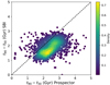 |
Fig. A.1. Comparison of t90−t50 estimated by our SBI method and Prospector in (Kaushal et al. 2024), for all galaxies in the selected sample described in Appendix A.1. |
Finally, in Fig. A.2 we show the mass dependency of the t90−t50 statistics, as also presented in Kaushal et al. (2024), and we confirm that both methods are compatible with a constant t90−t50 mass range 10.25<log M*/M⊙<12 for this small sample of galaxies.
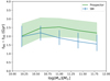 |
Fig. A.2. Variation of t90−t50 as a function of mass, estimated with Prospector (green) by Kaushal et al. (2024), and with our SBI method (blue). Error bars and shaded regions represent the 16th-84th confidence intervals. |
A.2. The Park et al. (2024) galaxy sample
We now compare our estimates with individual galaxies in Park et al. (2024). They studied 151 galaxies in the COSMOS field using data from the Blue Jay survey, a JWST Cycle 1 program (GO 1810; PI: Belli). After performing a spectro-photometric SED fit using Prospector on each galaxy, they selected 16 massive quiescent galaxies for which they have both NIRSpec spectroscopy (and spectroscopic redshifts) and photometry from HST/ACS+WFC3 and IRAC bands from Spitzer. Massive galaxies were selected with a cut at log M*/M⊙>10.0 and as quiescent with an sSFR one dex below the star forming main sequence from Leja et al. (2022). They carried out SED fitting with two different SFH priors: (1) the ‘continuity’ prior which uses a Student-T distribution with σ = 0.3 and ν = 2.0 (Leja et al. 2019), and (2) the ‘bursty’ prior from (Tacchella et al. 2022b), with σ = 0.1 which allows larger changes in star formation between two consecutive time bins.
We identified the same 16 galaxies in COSMOS2020. We rejected eight of them for either missing one of our photometric bands or being rejected by our outlier detection pipeline. Because our aim is to assess the performance of our method using a specific set of assumptions, we simply remove these galaxies and compare the remaining eight galaxies7
The green lines in Fig. A.3 shows the SFH estimated by (Park et al. 2024) using the continuity prior in green and the bursty prior (in pink) compared to our reconstruction (black). Since our method estimates only the normalised SFH, we used the stellar mass from (Weaver et al. 2022) to rescale them. We observe that the SFHs recovered with our method overall share the same shape across the sample (except for the peculiar COSMOS-8469), which is consistent with the selection of quenched galaxies and the homogeneity of massive quenched galaxies’ SFH described in 3.4.
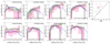 |
Fig. A.3. Comparison of SFH estimates for individual galaxies in the Park et al. (2024) sample. The shaded green regions shows the results using the continuity prior, in pink using the bursty prior, and in black our SBI estimate. The blue line shows the average SFH of passive galaxies. The size of the shaded regions corresponds to the 68% confidence intervals. The top right panel shows the median residuals between the the Park et al. (2024) estimates and either our SBI estimate (horizontal axes) or the average passive SFH (vertical axes). The points above the diagonal line indicate our method is closer to Prospector's estimate than the average passive SFH is. |
Our estimates agree broadly with (Park et al. 2024) despite our smaller credible intervals. In particular, COSMOS-8469's recovered SFH is always consistent with a constant SFH, despite the overall stellar mass appearing to vary significantly between fits. The galaxy formation ages are broadly consistent despite the fact that no redshift information is used in our fit. Interestingly, our method correctly estimates the age of formation of COSMOS-10400 at around 3 Gyr despite a significant difference between the spectroscopic redshift (z∼2.1) and the photometric redshift estimated by LePHARE (z∼0.99).
Finally, we compute the average SFHs of passive galaxies in the range 1.6<z<2.7 (in blue). We compare this naive estimate from our SBI one with Prospector by computing their respective distances; this is shown on the top right panel of Fig. A.3. In each case, for SBI, we computed the median distance between Prospector's estimates and 50 draws in the posterior distribution. This shows that SBI is consistently closer to Prospector than the naive estimate, which is particularly striking for the peculiar COSMOS-8469 object.
Appendix B: SBI sensibility to noise
In order to assess the sensibility of our approach to photometric noise, we run the following experiment: For a given galaxy in the HORIZON-AGN simulation, we have access to the noiseless fluxes. We draw a random sample of 100 noise variances in each filter and sort them in ascending order. We then compute the corresponding noisy fluxes to get a 100 mocks with increasing noise in every band but the exact same SFH. We finally use our estimator on each mock galaxy to infer the times of mass formation ti. Fig. B.1 shows the standard deviation of the estimation error between the truth and the posterior mean as a function of the noise (averaged over all filters). Fig. B.1 shows the standard deviation of the estimated posterior distribution (averaged over all ti as a function of the same noise. As expected, as the noise increase, σerr increases (the posterior mean gets further from the truth), and the variance of the posterior (i.e the size of the error bars on the estimates) also increases.
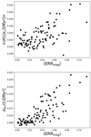 |
Fig. B.1. Evolution of the estimated posterior standard deviation σ(ti|xc) (Top) and of the estimation error (bottom) as a function of the photometric uncertainties. σ(ti|xc) and σerr(ti) are computed by applying an increasing level of noise to the same simulated galaxy and estimating the posterior for the SFH with our SBI approach. |
Appendix C: On the choice of the number of Lookback times N
Here we examine the role of the number of Lookback times N to be estimated. Since N controls the number of points on the cumulative mass function to be interpolated, increasing it decreases the interpolation error (see Fig. C.1(Top) for the SFH reconstruction and the orange points in Fig. C.1(Bottom) for the corresponding distance between the black SFH and each approximation). However, this increase also requires a higher dimensional output for the Neural Density estimator, corresponding to finer details of the SFH, making it computationally more challenging. As expected, the estimation error by the neural network increases with N (see the blue dots on Fig. C.1 (Bottom)). The choice of N therefore results in a trade-off between the approximation error due to the linear interpolation of the cumulative mass function and the estimation error due to the Neural Network. We highlight that N is not strictly speaking a number of parameters in the usual Bayesian inference sense: the prior volume is entirely determined by the SFH sampling in the simulation, which doesn’t depend on N. The ti are clearly not a priori independent, and their prior correlation structure depends on the HORIZON-AGN simulation, contrary to (Iyer et al. 2019) where it is defined by the Gaussian Process kernel.
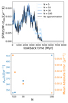 |
Fig. C.1. Top: Comparison of the reconstruction after interpolating the cumulative mass function for different values of N. Bottom: Illustration of the trade-off between the estimation error and the interpolation error as a function of N. The left axis shows the standard deviation of the different between the estimated and the true ti, while the right axis shows the mean absolute error between true normalised SFH and the reconstruction after interpolation for each value of N. |
Appendix D: Quality assessment of the summary quantities build from the SFH
In Section 4.2 we presented several summary statistics from the SFH: the slope, the number of peaks and the formation age (see Fig. 9). To assess the quality of these estimators, Fig. D.1 shows the comparison between these quantities derived from the reconstructed SFHs in HORIZON-AGN and those measured on the ‘true’ SFHs in the simulations. For the reconstructed SFH, the summary statistics are measured on 50 individual realisations from the posterior distribution, and then averaged. The mean number of peaks is generally biased towards lower values, although the hierarchy is correctly recovered. The reconstructed and intrinsic formation ages and slopes are reasonably well correlated.
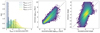 |
Fig. D.1. Comparison of the number of peaks, formation age and slope on reconstructed SFHs and intrinsic SFHs in the HORIZON-AGN simulation. For the reconstructed SFHs, the summary statistics are measured on 50 individual realisations from the posterior distribution and then averaged. |
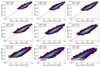 |
Fig. D.2. Comparison between the true formation times and our estimates, decile by decile, on ∼85000 galaxies randomly drawn in the Horizon-AGN simulation and not used in the training of the neural network. |
All Tables
All Figures
|
Fig. 1. Average distributions of SFHs in HORIZON-AGN. The ribbons show 95% intervals. |
| In the text | |
|
Fig. 2. Examples of the effect of our parametrisation on our HORIZON-AGN galaxies. The original SFH binned linearly (blue), and the reconstruction after interpolating between 30 mass quantiles computed directly on the true SFH (orange). |
| In the text | |
|
Fig. 3. Example of the quantities estimated by our neural network for a randomly selected galaxy in HORIZON-AGN. The true SFH is shown in blue, the estimated mean is plotted in orange, and the 95% confidence interval is shown in red. The mass quantiles estimated by the neural network are shown on the left, and the resulting reconstruction is presented on the right. The SFHs in grey are drawn from the estimated posterior distribution. |
| In the text | |
|
Fig. 4. Left: Comparison between the true formation times and the estimated posterior mean in HORIZON-AGN. Perfect inference would lie on the (blue) diagonal line. Our method yields an unbiased estimator with regard to HORIZON-AGN for all timescales. Right: Assessment of the estimated uncertainty calibration with the credibility level on the x-axis, and the realised coverage on the y-axis. For each level (50%, 68%, and 95%), the true value lay in the estimated credibility interval slightly more often than the expected level. A perfect uncertainty calibration would be on the blue diagonal. Our estimator is well calibrated. |
| In the text | |
|
Fig. 5. Normalised mass distributions of galaxies in our COSMOS2020 sample. Top: Star-forming galaxies. Bottom: Passive galaxies. The mass distribution of all galaxies in COSMOS (meeting requirements of observed bands, depth, and S/N; see Section 2) is darker and highlights potential biases in our selected sample after outlier rejection (lighter). |
| In the text | |
|
Fig. 6. Star formation rate and redshift of galaxies in the COSMOS2020 catalogue that were rejected by our prior predictive check, as a function of their mass. Galaxies that were classified as outliers (see Section 3.3) were excluded from our sample because they are too different in the colour space from the galaxies represented in HORIZON-AGN. |
| In the text | |
|
Fig. 7. Median SFHs of star-forming (dashed blue lines) and passive (solid red lines) galaxies in COSMOS2020 in several redshift ranges and decomposed into three mass bins, as indicated in the panels. The number of galaxies used to compute the median trend is indicated in the legend. The vertical grey shaded area (whose width depends on the considered redshift range) indicates the maximum look-back time above which the start of the SFH is not compatible with the age of the Universe. |
| In the text | |
|
Fig. 8. Evolution of the estimated SFHs for galaxies at redshift 0.5<z<1 in COSMOS2020 as a function of their position in the NUVrJ diagram. Top: Four galaxy populations are selected in the star-forming region (blue and clear boxes) and in the passive region (red box). Bottom: Estimated SFHs of galaxies in each box (same colours). |
| In the text | |
|
Fig. 9. Illustration of our method for measuring the formation age ageform, slope, number of maxima, and age of the first peak for an individual SFH drawn from the posterior distribution of each galaxy. The left panel shows two realisations of the SFH for the same galaxy from the COSMOS2020 catalogue (purple and cyan lines, smoothed with a Gaussian kernel with a standard deviation 100 Myr), together with the median over 50 realisations (grey line). The dashed vertical line indicates ageform, which was then used to compute the slope (solid straight segments). The circles indicate the position of the persistent maxima. The middle and right panels show the histograms of the numbers of maxima and slopes over 50 realisations. |
| In the text | |
|
Fig. 10. Slope of the reconstructed SFH, as defined in Equation (3) in COSMOS2020 (solid black lines with error bars) and HORIZON-AGN (dashed red lines) for all galaxies in the sample (top) and passive only (bottom). For each galaxy, individual slopes computed from 50 SFHs drawn from the posterior distribution were averaged. The two first redshift ranges were chosen to encompass similar comoving volumes in order to mitigate possible cosmic variance effects in the galaxy distribution. The hexagons are colour-coded by the logarithm of the galaxy number density in COSMOS2020 in the considered redshift bin. |
| In the text | |
|
Fig. 11. Number of maxima 〈m〉 in the COSMOS (top) and Horizon-AGN (bottom) SFHs as a function of stellar mass, colour-coded by the formation look-back time for two different redshift bins. The number of maxima is computed as described in Section 4.2.3 and Fig. 9. |
| In the text | |
|
Fig. 12. Formation epoch tU,form (i.e. the age of the Universe corresponding to the mass-weighted age of the galaxy as defined in Equation (2)) vs. mass in COSMOS2020 at 0.9<z<1.4 compared to the literature for all galaxies (left) and passive galaxies alone (middle). The right panel displays the age of the Universe corresponding to the first peak in the SFH. The black line shows the best-fit for the passive galaxies in COSMOS2020, and the red line shows the best-fit in HORIZON-AGN. |
| In the text | |
|
Fig. 13. Formation epoch tU,form (left) and age of the Universe at the first peak (middle and right) as a function of the redshift at which the galaxies are observed (or the corresponding age of the Universe) for passive galaxies in COSMOS2020. The hexagons are colour-coded by density (left and middle) or stellar mass (right). |
| In the text | |
|
Fig. 14. NUVrJ diagrams showing the separation of active and passive galaxies in 0.5<z<1 in COSMOS2020. The dashed line is from Ilbert et al. (2013). Top left: Fraction of passive galaxies (colours) selected as those with a LePHARE estimate of log(sSFR/yr−1)<−11. Top right: Same fraction from sSFRs estimated by our SBI method using all filters. Bottom left: Distribution of dust, as estimated by LePHARE. Bottom right: Same fraction from sSFRs estimated by our SBI method, but without the H Band. The SFH inferred by SBI without the H band on the right side of the panel corresponds to more passive galaxies than estimated with an SED fitting, which identifies these galaxies as active, but dusty. |
| In the text | |
|
Fig. A.1. Comparison of t90−t50 estimated by our SBI method and Prospector in (Kaushal et al. 2024), for all galaxies in the selected sample described in Appendix A.1. |
| In the text | |
|
Fig. A.2. Variation of t90−t50 as a function of mass, estimated with Prospector (green) by Kaushal et al. (2024), and with our SBI method (blue). Error bars and shaded regions represent the 16th-84th confidence intervals. |
| In the text | |
|
Fig. A.3. Comparison of SFH estimates for individual galaxies in the Park et al. (2024) sample. The shaded green regions shows the results using the continuity prior, in pink using the bursty prior, and in black our SBI estimate. The blue line shows the average SFH of passive galaxies. The size of the shaded regions corresponds to the 68% confidence intervals. The top right panel shows the median residuals between the the Park et al. (2024) estimates and either our SBI estimate (horizontal axes) or the average passive SFH (vertical axes). The points above the diagonal line indicate our method is closer to Prospector's estimate than the average passive SFH is. |
| In the text | |
|
Fig. B.1. Evolution of the estimated posterior standard deviation σ(ti|xc) (Top) and of the estimation error (bottom) as a function of the photometric uncertainties. σ(ti|xc) and σerr(ti) are computed by applying an increasing level of noise to the same simulated galaxy and estimating the posterior for the SFH with our SBI approach. |
| In the text | |
|
Fig. C.1. Top: Comparison of the reconstruction after interpolating the cumulative mass function for different values of N. Bottom: Illustration of the trade-off between the estimation error and the interpolation error as a function of N. The left axis shows the standard deviation of the different between the estimated and the true ti, while the right axis shows the mean absolute error between true normalised SFH and the reconstruction after interpolation for each value of N. |
| In the text | |
|
Fig. D.1. Comparison of the number of peaks, formation age and slope on reconstructed SFHs and intrinsic SFHs in the HORIZON-AGN simulation. For the reconstructed SFHs, the summary statistics are measured on 50 individual realisations from the posterior distribution and then averaged. |
| In the text | |
|
Fig. D.2. Comparison between the true formation times and our estimates, decile by decile, on ∼85000 galaxies randomly drawn in the Horizon-AGN simulation and not used in the training of the neural network. |
| In the text | |
Current usage metrics show cumulative count of Article Views (full-text article views including HTML views, PDF and ePub downloads, according to the available data) and Abstracts Views on Vision4Press platform.
Data correspond to usage on the plateform after 2015. The current usage metrics is available 48-96 hours after online publication and is updated daily on week days.
Initial download of the metrics may take a while.