| Issue |
A&A
Volume 699, July 2025
|
|
|---|---|---|
| Article Number | A72 | |
| Number of page(s) | 14 | |
| Section | The Sun and the Heliosphere | |
| DOI | https://doi.org/10.1051/0004-6361/202451747 | |
| Published online | 27 June 2025 | |
Response of energetic neutral atom flux in the heliosheath to fast variations in the solar wind and its dependence on pickup ion distribution models
Department of Astronomy and Space Science, Chungbuk National University, Chungbuk 28644, Republic of Korea
⋆ Corresponding author: This email address is being protected from spambots. You need JavaScript enabled to view it.
Received:
1
August
2024
Accepted:
13
May
2025
Abstract
Context. Interstellar Boundary Explorer images have revealed a globally distributed flux of energetic neutral atoms (ENAs) at ∼0.2–6 keV while Cassini observed an ENA belt at 5–55 keV likely originating from the inner heliosheath (IHS) protons via charge exchange with penetrating interstellar neutrals. Such ENAs are considered to reflect solar wind variations to some extent.
Aims. We explore ENA flux sensitivity in the IHS to solar wind changes at Carrington rotation (CR) resolution and quantify its dependence on IHS ion distributions.
Methods. We utilized three models for ion distributions designed to respond to solar wind changes upstream of the termination shock (TS), from which the corresponding variations in ENA fluxes were computed. All three ion models employ a regularized kappa distribution for solar wind protons. The models differ in the treatment of transmitted pickup ions (PUIs) and reflected PUIs with different combinations of regularized kappa and filled-shell distributions.
Results. Our ENA estimates reveal the potential for substantial flux change rates between adjacent CR times, often exceeding several tens of percent, a feature not recognized in previous studies. Such rapid variations in ENA flux levels exhibit a correlation with concurrent fluctuations in solar wind speed and density upstream of the TS. However, the specific characteristics of these ENA changes are contingent on the ion distribution model and the energy considered. Most notably, employing the filled-shell distribution for transmitted PUIs induces noticeable alterations in ENA flux near their cutoff energy (∼0.5–1.5 keV), responding promptly to rapid variations in solar wind bulk speed. Furthermore, the inclusion of reflected PUIs is critical in the high-energy regime (> ∼10 keV), which is typically associated with coronal hole fast streams, where ENA fluxes exhibit strong correlations with changes in the solar wind bulk speed and dynamic pressure.
Conclusions. The results underscore the importance of precise PUI information in the IHS for accurate ENA estimation during swift solar wind changes.
Key words: Sun: heliosphere / solar wind / ISM: atoms
© The Authors 2025
 Open Access article, published by EDP Sciences, under the terms of the Creative Commons Attribution License (https://creativecommons.org/licenses/by/4.0), which permits unrestricted use, distribution, and reproduction in any medium, provided the original work is properly cited.
This article is published in open access under the Subscribe to Open model. This email address is being protected from spambots. You need JavaScript enabled to view it. to support open access publication.
1. Introduction
The inner heliosheath (IHS) is the region where the generation of energetic neutral atoms (ENAs) is anticipated to occur through the charge exchange between ions and mostly interstellar neutral atoms. Ions from the solar wind emitted by the Sun along with pickup ions (PUIs) formed through processes such as charge exchange or photoionization (Vasyliunas & Siscoe 1976; Möbius et al. 1985; Geiss et al. 1994; Gloeckler et al. 1997; Randol et al. 2013; McComas et al. 2017a, 2021) travel outward in tandem with the bulk solar wind flow. They penetrate the IHS via the termination shock (TS). Within the IHS, some of these ions undergo transformation into ENAs through charge exchange with interstellar neutrals. Upon their return journey toward Earth, ENAs originating from the IHS become observable. All of these processes are demonstrated in the schematic shown in the top panel of Fig. 1. Interstellar Boundary Explorer (IBEX) images have indicated a background ENA flux, referred to as the globally distributed flux (GDF), at 0.2–6 keV, which is attributed to termination-shock-heated protons in the IHS (Funsten et al. 2009; McComas et al. 2009; Schwadron et al. 2011). Cassini spacecraft observations have revealed an ENA belt at approximately 5–55 keV likely originating from energetic protons in the IHS (Krimigis et al. 2009; Dialynas et al. 2013).
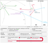 |
Fig. 1. (Upper panel) Schematic illustration of the core concept behind the interaction between solar radiation, solar wind protons, and interstellar neutrals leading to the formation of pickup ions through ionization and/or charge exchange in the supersonic solar wind. Pickup ions are tied to the heliospheric magnetic field and are transported outward by the solar wind. These processes generate energetic neutral atoms via charge exchange between solar wind protons, pickup ions, and interstellar neutrals in the inner heliosheath – the region between the termination shock and the heliopause. The outer heliosheath is the region in the very local interstellar medium adjacent to the heliopause. (Lower panels) Overview of the current understanding of ion distributions in the inner heliosheath, the availability of bulk solar wind data, and a flowchart summarizing the main ideas of the study. |
These ENAs are considered to reflect variations in the solar wind to a certain degree (McComas et al. 2017b, 2020). Notably, ecliptic and off-ecliptic solar wind observations by Voyager suggest a factor of two variation in solar wind dynamic pressure with the solar cycle (Lazarus & McNutt 1990; Richardson 1997). Schwadron et al. (2018) propose that changes in the solar wind dynamic pressure drive GDF evolution within 40° of the upwind pressure maximum through compression and rarefaction in the heliosheath. Reisenfeld et al. (2012, 2016) capitalized on the continuous coverage of the polar ENA flux originated from the IHS and proposed two key insights: (i) variations in the solar wind dynamic pressure impact the TS, initiating pressure waves that propagate through the IHS at the local magnetosonic speed, thereby influencing the flux of ENAs formed in this region, and (ii) a temporal structure present in the pre-TS solar wind may persist in the shocked plasma streaming through the IHS, subsequently imprinting on the ENAs.
Several simulations have explored the impact of solar wind variations on the outer heliosphere (Zank & Müller 2003; Scherer & Fahr 2003a,b; Fahr & Scherer 2004; Zirnstein et al. 2015; Schwadron & McComas 2019). Zank & Müller (2003) conducted an investigation into the heliosphere’s response to temporally varying solar wind using a multifluid model that incorporates the charge-exchange interaction between neutral hydrogen and protons in a self-consistent manner. This study considered both variable solar cycle dynamic pressure and the presence of disturbances with a global extent, such as globally merged interaction regions, which are produced by interaction among a series of transient streams and other flows over a period of only a few solar rotations or more (see Fig. 5 in Burlaga 2015). The findings indicated that the large-scale heliosphere is likely to be highly time dependent and dynamic. Furthermore, simulations by Washimi et al. (2007) revealed that variations in solar wind dynamic pressure caused by interplanetary shock waves lead to the displacement of the TS from its steady-state equilibrium position, resulting in the emission of shocks and waves downstream. Disturbances transmitted or emitted from the TS to the heliopause (HP) undergo partial reflection at the HP, and the reflected waves return, colliding with the TS. This highlights the significance of solar wind variability in influencing the dynamics of the global heliosphere, including the potential impact on IHS ion dynamics and, ultimately, variations in ENA flux. Additionally, Scherer & Fahr (2003a,b) and Fahr & Scherer (2004) simulated the outer heliospheric responses to long-term variations of the solar wind by employing a set of time-dependent models of the solar wind speed and density at the inner boundary of their simulations (at r = 5 AU, to be consistent with observations from Ulysses). Their simulation model included a coupling among five fluids, that is, protons, H-atoms, PUIs, anomalous cosmic rays, and galactic cosmic rays. In particular, the work by Fahr & Scherer (2004) included evolution of PUIs along the plasma stream lines in the IHS in an approximated way.
Therefore, this complex interplay between varying solar wind conditions and the temporal variability of ENA flux merits definitive investigation (Zirnstein et al. 2015). In the current investigation, our focus is twofold. Firstly, we intend to scrutinize the responses of ions within the IHS and the ensuing ENA fluxes to rapid variations in solar wind, particularly at Carrington rotation (CR) timescales. Secondly, we explore the substantial impact of specific ion distributions in the IHS on observed ENA fluxes. The essence of the main idea of our investigation is summarized in Fig. 1.
Observations and prevailing theories jointly propose that as outflowing ions cross the TS, the heliosheath ion distribution becomes a mixture of transmitted solar wind ions and energized PUIs. Notably, we underscore the unique feature of PUI distributions having a discernible cutoff at twice the solar wind speed in the solar inertial frame. For instance, New Horizons observations at ∼46 AU found cutoff energies of ∼2.8 keV for H+ and ∼10.4 keV for He+, which is approximately four times the peak energies of the corresponding solar wind ions (McComas et al. 2017a, 2021). Additionally, Voyager observations have indicated changes in the solar wind proton temperature from ∼2 × 10⁴ K upstream to ∼1.8 × 10⁵ K downstream (Richardson et al. 2008). Downstream temperatures estimated by Zank et al. (2010) for solar wind protons, transmitted PUIs, and reflected PUIs transmitted downstream at ∼1.25 × 10⁵ K, ∼9.75 × 10⁶ K, and ∼7.7 × 10⁷ K, respectively.
In our examination, we employed three distinct models for ion distributions within the IHS, utilizing them to compute ENA fluxes in a straightforward manner. Our focus lies in understanding the responses of these ion distributions to rapidly changing solar wind conditions upstream of the TS, derived from a model based on observations at 1 AU. We highlight the distinctions in ENA responses arising from three distinct ion distribution models and delve into their implications. Our aim is that this research proves valuable by offering insights into the evolution of heliospheric ENA with a temporal resolution significantly shorter than that achieved by IBEX, thus aligning with the anticipated capabilities of the upcoming the Interstellar Mapping and Acceleration Probe (IMAP) mission to some extent (McComas et al. 2018).
Section 2 details the methods used, Section 3 presents the main results, and Section 4 discusses critical issues.
2. Methodology
2.1. Ion distributions in the IHS
The calculations of the heliospheric ENA fluxes have been performed using various methods in numerous previous studies (Gruntman et al. 2001; Heerikhuisen et al. 2007, 2014; Izmodenov et al. 2009; Fahr et al. 2011; Siewert et al. 2012; Schwadron & McComas 2013; Möbius et al. 2013; Zirnstein et al. 2015; Swaczyna et al. 2016; Gamayunov et al. 2017). Here we adopted the expression for ENA fluxes expressed as (e.g., Fahr & Scherer 2004; Livadiotis et al. 2012)
 (1)
(1)
where ε is the ENA energy in the inertial reference frame of the heliosphere, measurement time t is in units of CR, τ refers to the retarded time discussed below,  is the survival probability of ENAs from their source to Earth, which is given by
  (Livadiotis et al. 2011), σex is the cross section for charge exchange between protons and interstellar hydrogen atoms (Lindsay & Stebbings 2005), and nH is the number density of interstellar neutral hydrogen, taken as 0.09 cm−3 (Bzowski et al. 2009). The jion is the ion flux in the IHS, which is defined by
 (2)
(2)
where m is the ion mass, nion is the number density of specific ion population, fion is the ion distribution, and u is the individual ion velocity in the inertial reference frame of the heliosphere. It should be emphasized that both nion and fion can vary radially as well as in other directions in the IHS. In the present work, we restrict ENA calculations in Eq. (1) to the noseward direction on the equatorial plane.
To obtain ENA fluxes at a given measurement time t near the Earth and energy ε from Eqs. (1) and (2), we follow the steps outlined below. First, we derive the solar wind speed and density just upstream of the TS (at r = 90 AU) by transmitting the 1 AU observations using a straightforward solar wind model of Lee et al. (2009). This is performed for solar wind parcels identified at the CR time resolution. The details of this step are described in Sect. 2.2 below. From this, fion in the IHS are expressed as a function of the solar wind speed and density upstream of the TS, as described later in this section. Second, we evaluate Eq. (1) for three specific models for fion also described below in this section. Importantly, we stress that jion in the integral of Eq. (1) is evaluated at the retarded time τ, which is defined by
 (3)
(3)
This formulation accounts for two effects: (i) the convection time of a downstream solar wind parcel (corresponding to each CR) traveling from the TS to a charge exchange point r within the integral in Eq. (1) (where ENAs are generated) at the downstream bulk speed (ub, ds) (second term on the right-hand side); and (ii) the travel time of the generated ENA particle from its generation point r back toward to the Earth observer moving at a speed corresponding to its energy (third term on the right-hand side). Note that in effect (i), each solar wind parcel delivers the upstream conditions that ultimately determine fion at the specific location r within the IHS. For practical implementation of effect (i), we assume that all solar wind parcels are transported throughout the IHS at a uniform speed of 200 km/s. This effectively allows a mixture of solar wind parcels spanning about 10 CRs. While this simplification aids tractability, it omits more realistic complexities such as flow stream bending near the heliopause and potential disturbances by globally merged interaction regions, if present.
On the other hand, the number of ions that can contribute to generation of ENAs is expected to decrease with distance from the TS due to charge exchange losses during the convection across the IHS. Indeed, the radial dependence of ion number density in the IHS, particularly due to charge exchange, has been recognized (Heerikhuisen et al. 2019; Shrestha et al. 2021; Bera et al. 2023). In the present work, we account for this effect by using the following expression taken from Heerikhuisen et al. (2019):
 (4)
(4)
where nds and ub, ds are the ion number density and solar wind bulk speed just downstream of the TS, respectively. This equation represents the accumulated losses up to a given r due to charge exchanges experienced by bulk plasma while moving from the TS to r. By using this expression, we intend to reflect the convection effect in a simplified way (assuming no diffusion effects by turbulence and waves and neglecting freshly injected PUIs), as discussed in Fahr & Scherer (2004).
The ion distribution can be notably influenced by several processes, including wave and turbulence (e.g., Gamayunov et al. 2012) and charge exchange (e.g., Heerikhuisen et al. 2019). This implies a possible radial dependence in the IHS (see Eq. (6) and related description below). However, due to challenges in distant observation, uncertainties persist, and questions remain regarding relative significance of ion populations and their distributions. Consequently, various attempts have been made to characterize the ion distributions, with proposals including Maxwellian, standard or regularized kappa, or filled-shell distributions by different authors (Zank et al. 2010; Livadiotis et al. 2012; Zirnstein et al. 2014; Kornbleuth et al. 2018; Scherer et al. 2022). To effectively address the complexity arising from solar wind conditions, we consider three model combinations for the distribution of solar wind ions and PUIs.
As outlined in Table 1, we explore three models for IHS ions, considering protons only, and examine three populations of protons. First, proton populations originating from the Sun are included in all three models. While the cold core population of these solar wind protons should be well described by a Maxwellian distribution, suprathermal protons in the solar wind may exist and can be described by a kappa distribution (Pierrard & Lazar 2010; Livadiotis et al. 2018; McComas et al. 2022). Particularly in the IHS, we allow for the possible existence of a non-negligible amount of accelerated or heated solar wind protons. Previous works have utilized the standard or regularized kappa distributions for such protons in the IHS (Prested et al. 2008; Heerikhuisen et al. 2008, 2019; Livadiotis et al. 2012; Scherer et al. 2022). In all three models considered in this study, we employed the isotropic regularized kappa distribution for solar wind protons. The regularized kappa distribution, introduced by Scherer et al. (2017), is a generalized form of the standard kappa distribution (Vasyliunas 1968; Pierrard & Lazar 2010). This formulation resolves issues inherent in the standard kappa distribution such as diverging velocity moments and unphysical constraints on the range of permissible kappa values (Scherer et al. 2017, 2019; Lazar & Fichtner 2021). (A more detailed description on the regularized kappa distribution is provided in Eq. (5)).
Three models for proton distribution in the inner heliosheath.
Second, we consider transmitted PUIs, which are modeled as the filled-shell distribution in Models 1 and 2. This distribution is widely recognized as characteristic of PUIs in interplanetary space (Vasyliunas & Siscoe 1976; Zank et al. 2010; McComas et al. 2021). In contrast, Model 3 adopts the regularized kappa distribution for this component. This adoption in Model 3 allows for the possibility that, as the PUIs pass through the TS, the originally filled-shell distribution of PUIs in the upstream solar wind changes to a regularized kappa distribution with a higher temperature in the IHS.
Lastly, we consider the reflected PUIs that are accelerated through the TS due to the cross-shock electrostatic potential of a quasi-perpendicular shock (Zank et al. 2010; Zirnstein et al. 2014). Reflected PUIs are excluded in Model 1 but are incorporated in Models 2 and 3, modeled as the regularized kappa distribution with even higher temperatures (see Eq. (7) and Fig. 3d).
Therefore, we emphasize that since the solar wind protons maintain identical distributions across all models, the distinctions between the three models in the ENA flux are contingent on the distribution of pickup protons. Specifically, the three models are distinguished by the following two aspects:
(i) Significance of reflected PUIs distribution: Model 1 and 2 differ in their treatment of reflected PUIs. Model 1 excludes them entirely, whereas Model 2 incorporates them to highlight their significance. For both models, however, the distributions for solar wind protons and transmitted PUIs are identical.
(ii) Significance of transmitted PUIs distribution: Model 2 and 3 differ in the assumed distribution for transmitted PUIs. Model 2 adopts a filled-shell distribution, whereas Model 3 employs a regularized kappa distribution. In both models, the distributions for solar wind protons and reflected PUIs are assumed to be the same. Comparison of the results from these two models underscores the significant impact of the filled-shell distribution on the outcomes.
The isotropic regularized kappa distribution in the IHS is expressed as (Scherer et al. 2022)
 (5)
(5)
where  with a normalization speed Θ, ξ is the cutoff parameter
  , κ is the kappa index, and U(a,b,z) is the Kummer-U function (Abramowitz & Stegun 1970). We adopted κ = 2 as a representative value (Livadiotis et al. 2011). For smaller values of κ, the κ-distribution yields a greater number of particles at higher energies. Consequently, if the core solar wind population is modeled with a small κ value, it begins to dominate over PUI populations in the high-energy regime and thus effectively overshadows the contribution of PUIs, which are modeled separately according to the distribution model types in Table 1. However, Voyager observations imply that PUIs constitute a significant fraction of the ion populations, especially at higher energies. Therefore, adopting an overly small κ value diminishes the PUI role and is not consistent with the observational constraint. By choosing κ = 2, we aim to better represent reported observations.
Note that in the limit of ξ = 0 in Eq. (5) the standard kappa distribution can be recovered. Choosing a specific finite ξ value suitable for IHS ions under consideration requires justification. For this purpose, we rely on recent work by Scherer et al. (2022), who performed a direct fit to the measured ion spectra in the IHS for an extended energy range of 0.11–344 MeV. The ion spectra were derived from various measurements, including protons in the range of 0.11–55 keV (converted from remotely sensed ENA measurements from the IBEX and Cassini) and 28 keV–344 MeV (in-situ ion measurements from Voyager 2). The fitting was conducted using regularized kappa distributions applied to the average ion spectra for two time-intervals, 2009–2012 and 2013–2016, respectively. Their successful fitting required combinations of three regularized kappa distributions for the 2009–2012 spectrum and six for the 2013–2016 spectrum. The cutoff parameter ξ in these fits ranged from 1 × 10⁻⁴ to 6.59 × 10⁻².
We emphasize that the range of the ξ values in Scherer et al. (2022) were obtained for “average ion spectra over 4 years”, whereas our work focuses on ion spectra that may vary over much shorter timescales, about which no observational information is currently available. Furthermore, it is important to note that the 0.11–55 keV (the most relevant for our work) spectra in Scherer et al. (2022) were drawn from remotely measured ENA data rather than direct in situ measurements. This adds a degree of uncertainty in selecting an accurate value of the cutoff parameter ξ suitable for our study. Nevertheless, we consider the ξ values in Scherer et al. (2022) to be valuable, as they represent the only observationally based information available. In Scherer et al. (2022) their fittings with multiple regularized kappa distribution were applied to a broad energy range of 0.11–344 MeV, while our work is concerned with the narrower energy range of 0.1–50 keV where the ENAs of IHS origin have been measured by IBEX and Cassini. Within the energy range of 0.1–50 keV, the regularized kappa distributions in Scherer et al. (2022) are characterized by ξ values ranging from 3 × 10⁻² to 3.8 × 10⁻². For all the results presented below, we have taken ξ = 3.8 × 10⁻². However, from a technical perspective, the main conclusions of the present study remain unchanged for different values of ξ in this range.
In the present work, we use the distribution function (Eq. (5)) as expressed in the heliospheric inertial frame. This is done by converting the energy E = mp|u − ub, ds|2/2 in Eq. (5) to  . Here u is the particle’s individual velocity, and ub, ds is the solar wind bulk velocity in the downstream (that is, within the IHS), ε = mpu2/2, εb, us = mpub, us2/2 is the kinetic energy of bulk solar wind the upstream, R is the compression ratio (the ratio between the upstream and downstream bulk speeds, ub, us/ub, ds), and δ is defined by δ ≡ −cos(ω), where ω is the orientation angle between the solar wind proton velocity and bulk velocity (see Fig. 1 in Livadiotis et al. 2012 for details). We set ω = 180° to consider ENAs in the sunward direction only.
As we acknowledge a possible radial dependence of ion distributions in the IHS, we reflect this dependence by considering the possibility of varying temperature throughout the IHS. Currently, the observational information on temperature variability throughout the IHS is available only from Voyager 2 measurements (Richardson et al. 2023). However, the Voyager 2 measurements were made off the equatorial plane and more critically did not include PUI measurements, the contribution of which can be significant to ion temperature. Nevertheless, the monthly averaged data exhibits a decreasing temperature profile mostly over several AU after the TS followed by nearly a constant temperature. For the work here, we choose to utilize recent simulation results from which we construct a simple expression for the temperature with a radial dependence. Specifically, we use the 3D multifluid simulation results of Bera et al. (2023) which are based on ideal MHD for all charged particles with the source terms responsible for charge exchange between ions and neutral atoms and gas dynamic Euler equations for neutral populations. Their simulation results provide the radial profile of temperature throughout the IHS in which the temperature decreases as a function of distance in the IHS. The decrease is more pronounced nearer to the HP, unlike that seen in the profile from the Voyager 2 observations. To apply this simulation outcome to our work, we fit a cubic polynomial function to one of their temperature curves (Fig. 8 in their paper), resulting in the following analytic expression:
![Mathematical equation: $$ \begin{aligned} T(r)&=T_{\mathrm{ds} } [(-3.20175\times 10^{-5})\,r^3 + 0.00897\,r^2 \nonumber \\&\quad -0.83617\,r+26.93092], r_{\mathrm{TS} } < r < r_{\mathrm{HP} }, \end{aligned} $$](/articles/aa/full_html/2025/07/aa51747-24/aa51747-24-eq11.gif) (6)
(6)
where r is the distance in the IHS from the TS, and Tds refers to the temperature of each population just downstream of the TS. We apply this to all three ion populations. For solar wind protons and transmitted PUIs in the IHS, we take Tds = 105 K and 107 K, respectively. For the reflected PUIs in the IHS, we adopted the following expression for Tds (Zank et al. 2010), denoted as  :
:
![Mathematical equation: $$ \begin{aligned} T_{\mathrm{ds} }^{\mathrm{ref} } \simeq \frac{m_\mathrm{p} }{3k_{\mathrm{B} }} \left[1 + \frac{1}{4} \left(\frac{r_{\mathrm{gyro,us} }}{L_{\mathrm{ramp} }}\right)^2 \right] u_{\mathrm{b,us} }^2(\tau ), \end{aligned} $$](/articles/aa/full_html/2025/07/aa51747-24/aa51747-24-eq13.gif) (7)
(7)
where rgyro, us is the proton gyro radius in the upstream (∼63 000 km), and Lramp is the shock ramp thickness (5500 km). Notably  changes by the time-varying upstream bulk speed (further discussed in Sect. 2.2 below). Consequently, the regularized kappa distribution in the IHS is controlled by the upstream bulk speed (ub, us) and the compression ratio (R).
The filled-shell distribution has long been recognized and established as a representation of the PUI distribution in interplanetary space (Vasyliunas & Siscoe 1976). This distribution is distinguished by a cutoff energy, implying that PUIs are not observable above a certain energy threshold (McComas et al. 2017a, 2022). In the IHS, the filled-shell distribution is given by
![Mathematical equation: $$ \begin{aligned} f_{\mathrm{fs} }&=\frac{3}{8\pi } \cdot \varepsilon _{\mathrm{b,us} }(\tau )^{-\frac{3}{4}} \cdot \left(\frac{2}{m_\mathrm{p} }\right)^{-\frac{3}{2}} \cdot h^{-\frac{3}{2}} \cdot \nonumber \\&\quad \left[\varepsilon + \frac{\varepsilon _{\mathrm{b,us} }(\tau )}{R(\tau )^2}+ 2\sqrt{\varepsilon }\sqrt{\varepsilon _{\mathrm{b,us} }(\tau )} \cdot \frac{c}{R(\tau )}\right]^{-\frac{3}{4}} \cdot \\&\quad \Theta (\varepsilon _{\mathrm{cutoff} }(\varepsilon _{\mathrm{b,us} },h,R)-\varepsilon ),\nonumber \end{aligned} $$](/articles/aa/full_html/2025/07/aa51747-24/aa51747-24-eq15.gif) (8)
(8)
where h is the heating factor, defined by the maximum possible speed in the IHS, vMAX = h ⋅ ub, us (Livadiotis et al. 2012). The downstream temperature for the filled-shell distribution is expressed as  . This can be further cast into Tds = Tus R3/2h7/2 where
  . For practical purposes, we express the heating factor h in terms of the compression ratio R by adopting the relation
  for PUIs as given by Zank et al. (2010). Consequently, the heating factor h can be expressed as h = R1/7. The final part in Eq. (8), Θ, is a step function, and it is set to zero when the energy (ε) exceeds the cutoff energy (εcutoff). The cutoff energy is expressed as
![Mathematical equation: $$ \begin{aligned} \begin{array}{l} \varepsilon _\mathrm{cutoff} =\varepsilon _\mathrm{b,us} (t)\times \left[-\frac{c}{R(\tau )}+\sqrt{h^2-\frac{(1-c^2)}{R(\tau )^2}}\right]^2. \end{array} \end{aligned} $$](/articles/aa/full_html/2025/07/aa51747-24/aa51747-24-eq19.gif) (9)
(9)
Consequently, similar to the regularized kappa distribution, the filled-shell distribution in the IHS depends on the upstream bulk speed (ub, us) and the compression ratio (R). We caution readers that the dependence of the filled-shell distribution in Eq. (8) on the compression ratio R is valid only to the extent that the heating factor h can be approximated as h = R1/7, a simplification that, in turn, relies on the expression  for PUIs given by Zank et al. (2010).
Despite the simplification, we employed the well-known Rankine-Hugoniot jump conditions from MHD to evaluate the compression ratio. Assuming that the TS is approximately the perpendicular shock, one can derive the expression for R in terms of upstream Mach numbers as given in Eq. (10) (Burgess 1995):
 (10)
(10)
where  and
and  defined in the upstream of TS. For both Mach numbers, the determination of the magnetic field intensity (B) and thermal pressure (P) in the upstream of the TS is essential. However, continuous observational data for these parameters are lacking. To address this, we adopted a simplified model. In this model, near the TS, we assume that the frozen-in plasma flow is predominantly radial (u ≈ ur), and the magnetic field is primarily characterized by its azimuthal component with (B ≈ Bϕ) a latitudinal dependence of sin θ following the Parker spiral model. Under the assumption of a time-stationary state for an average background large-scale magnetic field in Faraday’s law, combined with the frozen-in condition, ∇ × (u × B) = 0, the following expression for the azimuthal component of heliospheric magnetic field is derived in a spherical coordinate system where (r, θ, ϕ) are the radial, co-latitude, and azimuthal component:
 (11)
(11)
The subscript 0 denotes the value at 1 AU. We stress that this formula is applicable to the region close to TS. We also emphasize that given ur, 0 from observations at 1 AU, Bϕ upstream near TS is a function of upstream bulk speed, ub, us. Although not explicitly shown here, we confirmed that the magnetic field level at 90 AU derived from Eq. (11) aligns with the Voyager 2 observations. For reference, Eq. (11) is similar to but not exactly same as the Parker’s spiral field expression given by  where Ωsun is the angular velocity of the solar rotation and
  for the bulk speed ub = 432 km/s. For the upstream thermal pressure, we utilize the model prediction values of solar wind density near the TS derived from those at 1 AU, as elaborated in Sect. 2.2 below, and we adopted an average value for the upstream temperature obtained from Voyager 2 observations, specifically
  . As a results, the compression ratio in our model is contingent upon the solar wind bulk speed and density in the upstream of TS.
In summary, Eqs. (8) and (9) depend on the compression ratio R, in addition to the heating factor h, which can also be expressed as a function of R. It is important to emphasize that the compression ratio R in Eq. (10) is determined exclusively by the two Mach numbers in the “upstream” region of the TS. Therefore, evaluating the Mach numbers requires knowledge of the magnetic field intensity, plasma density, temperature, and bulk speed, all measured in the upstream region of the TS. Ultimately, the compression ratio R is expressed as a function of the upstream bulk speed and density. Consequently, both the filled- shell distribution in Eq. (8) and the cutoff energy in Eq. (9) are also functions of these upstream parameters only.
Ultimately, we need the expression for the ion flux in the IHS, denoted as jion in Eq. (2), which necessitates the number density of a specific IHS ion population, nion. As mentioned above, the upstream solar wind density is obtained from a model prediction (see Sect. 2.2), subsequently determining the downstream solar wind density through the compression ratio. For the PUI density nPUI, we employed the fitting results derived from New Horizons observations (McComas et al. 2017a), suggesting the PUI density is proportional to the square root of the solar wind density. Given the lack of observational information about the PUI density in the IHS, we assume that this fitting result remains valid in this region. Practically, in our formulation of ENA flux calculations, the significance of the PUI density is introduced through the PUI density ratio relative to the total ion density, denoted as  . Additionally, we assume a relative ratio of 0.9 for transmitted PUIs and 0.1 for reflected PUIs. We emphasize that the PUI density ratio χ in the IHS is not fixed but varies over time in response to the upstream solar wind variations (demonstrated in Fig. 3 in Sect. 2.2 below).
To estimate the ENA fluxes predicted by each of the three models, we integrate the ion flux jion radially from the TS to the HP in Eq. (1), which incorporates radially varying ion number density and ion temperature in the IHS, as given in Eq. (4) and (6), respectively. In this calculation, we assume the TS to be at 90 AU and the HP at 120 AU, implying the IHS thickness of 30 AU. However, the IHS thickness can vary depending on the solar cycle, influenced by factors such as solar wind density, speed and cosmic rays (Whang & Burlanga 1993; Zank 1999; Zank & Müller 2003; Washimi et al. 2007; Manuel et al. 2015; Izmodenov & Alexashov 2020). We discuss the possible effects of different IHS thickness values in Sect. 4.
2.2. Extending solar wind from 1 AU to the vicinity of the termination shock
The ion distributions within the IHS discussed in Sect. 2.1 are contingent on the fluctuating solar wind conditions upstream of the TS, which, in turn, rely on conditions observed at 1 AU where most measurements are conducted. We note, for example, in a previous work by Scherer & Fahr (2003a,b) that they employed time-dependent models of the solar wind speed and density at the inner boundary of their 5 fluid simulations (at r = 5 AU, to be consistent with observations from Ulysses) to examine the outer heliospheric responses to long-term variations of the solar wind. For the purpose of our work here, we derive the needed solar wind speed and density upstream of the TS from those at 1 AU by employing a straightforward solar wind model given by Lee et al. (2009). This model is formulated based on mass-loading through photoionization and the loss of momentum and energy through charge exchange. It assumes a steady state and neglects solar gravity, solar magnetic field effects, and electron impact ionization. Specifically, the bulk speed (u) and number density (n) of the upstream solar wind at a given radial distance (r) is expressed as follows:
![Mathematical equation: $$ \begin{aligned} u&=u_\mathrm{0} -\left[1-\frac{1}{2}\frac{\gamma -1}{2\gamma -1}\right]\alpha r,\end{aligned} $$](/articles/aa/full_html/2025/07/aa51747-24/aa51747-24-eq29.gif) (12)
(12)
 (13)
(13)
where α = σexnH, ∞u0 + mpρ0−1(νH0nH, ∞+4νHe0nHe, ∞), u0 and ρ0 are the solar wind speed and mass density at 1 AU, respectively, γ is the ratio of specific heat, taking γ = 5/3, nH, ∞ and nHe, ∞ are the interstellar neutral hydrogen and helium densities, respectively, and νH0 and νHe0 are the photoionization rates at 1 AU for hydrogen and helium, respectively. We use the CR-averaged photoionization rates from the F10.7 flux (Sokół et al. 2020). The parameter α term provides insights into the frequency of charge exchange or photoionization events occurring from 1 AU to upstream of the TS.
In the present work, we restrict our ENA calculations to the noseward direction on the equatorial plane. Initially, the solar wind at 1 AU was obtained from OMNI data1, representing the in situ measurements near heliolatitude ≈0°. Since the provided solar wind data has an hourly time resolution, we averaged the data over each period corresponding to CR number to create monthly data. Then, using Eqs. (12) and (13) with nH, ∞ = 0.09 cm−3 (Bzowski et al. 2009) and nHe, ∞ = 0.015 cm−3 (Gloeckler et al. 2004), we calculated the transit time from 1 AU to the TS according to  , where TS was assumed to be at 90 AU. Since the physical parameters entering u(r) through Eq. (12) vary with CR times, the corresponding transit times differ accordingly. What moves behind can catch up with what is in front. Consequently, solar wind parcels, originating from different CR times at 1 AU, each experiencing different transit times, do not maintain their original sequential order upon arrival at the TS. Furthermore, the initial temporal resolution of one CR at 1 AU cannot be preserved at 90 AU. The values of the solar wind speed and density at both 1 AU and the TS are shown in Figs. 2b and 2c for the three solar cycles along with the sunspot number in Fig. 2a. We used the sunspot number provided by the Solar Influences Data Analysis Center2. The solar wind profiles at the TS (pink lines) in Figs. 2b and 2c start about one year later than those at 1 AU (black lines), as they are the result of applying the transit time to the solar wind data over three solar cycles. The solar wind values at the TS in Figs. 2b and 2c are on average similar to Voyager 2 observations in the upstream region (Vsw = 405 ± 34 km/s, NSW = 0.001 ± 0.0005 cm−3). In evaluating the ENA fluxes in Eq. (1), we identified the arrival time of solar wind parcels that best matches the retarded time from their re-ordered temporal sequence at the TS and used the corresponding solar wind parameter values to determine the ion distribution in the IHS.
 |
Fig. 2. (a) Sunspot number. (b) Solar wind speed and (c) Solar wind density at 1 AU (black) and 90 AU (pink) at a time resolution of Carrington rotation. In (b) and (c), the data at 1 AU are available from OMNI data center, while those at 90 AU were obtained by considering differing transit times of solar wind parcels of different CRs using the simplified model of Lee et al. (2009). Accordingly, the solar wind profile at 90 AU (pink) begins about one year later than the profile at 1 AU (black). (For more details, see the first two paragraphs of Sect. 2.2). |
2.3. Expressing IHS ion flux jion as a function of upstream solar wind variables
The ion flux expression for each ion population in the IHS, denoted by jion in Eq. (2), is governed by four parameters: the PUI density ratio (χ), the reflected PUI temperature (Tdsref), the cutoff energy (εcutoff), and the compression ratio (R). As demonstrated in Sect. 2.1, we emphasize that these parameters are a function of the upstream solar wind speed (ub, us) and/or the upstream solar wind density, both of which are time varying.
Figure 3 illustrates the time variations in the four parameters along with the upstream bulk speed across three solar cycles. Figure 3b shows the compression ratio, which is defined by Eq. (10) and computed by the method explained in the paragraph containing Eq. (10) in Sect. 2.1 above. It exhibits some dependence on the solar cycle despite different transit times of solar wind parcels, with values ranging from approximately 3.6 to below 4, displaying weak to modest variations. This range of values exceeds the compression ratio of 3 or less obtained from Voyager observations (Stone et al. 2005; Richardson et al. 2008). We have further investigated the sensitivity of the compression ratio to plasma temperature, the sole constant in our study. It has been confirmed that even with reasonable changes in temperature within the range measured by Voyager 2, the compression ratio consequently remains within the range from ∼3.6 to below 4. The other parameters in the IHS are shown in Figs. 3c, 3d, and 3e. The cutoff energy in the filled-shell distribution (εcutoff), Eq. (9) in Sect. 2.1 above, exhibits abrupt variations ranging between ∼0.5 and < 1.5 keV. The temperature of the reflected PUIs (Tdsref), Eq. (7) in Sect. 2.1 above, varies within a factor of ∼3, but stays above 108 K mostly. The relative density of PUIs (χ), defined by  as described in Sect. 2.1 above, lies within the range of ∼0.05 to ∼0.08. McComas et al. (2021) predicted, based on an extrapolation of New Horizons observations at 45 AU to the TS, that the relative density of PUIs to the total ion density increase linearly, reaching approximately 24% of the total ion density near the TS. However, caution should be exercised with this simple extrapolation, as the PUI ratio can be influenced by factors such as spherical expansion and the continuous addition of fresh PUIs. Considering the density jump across the TS and assuming no abrupt increase of PUIs in the IHS, the relative ratio of the PUIs in the IHS is expected to decrease by a few factors. The estimated ratio in Fig. 3e mostly aligns with this range of expectation. Frequently, both the reflected PUI temperature and the relative density of PUIs also undergo fast variations.
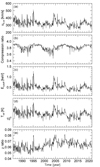 |
Fig. 3. (a) Solar wind bulk speed in the upstream of the termination shock. This is in fact the same data as the solar wind speed at 90 AU shown in Fig. 2b, repeated for convenience. (b) Compression ratio R defined by Eq. (10). (c) Cutoff energy of filled-shell distribution defined by Eq. (9). (d) Temperature of reflected PUI distribution defined by Eq. (7). (e) PUI density ratio relative to total ion density in the inner heliosheath, that is, |

3. Model calculation results
In this section, we present the ENA fluxes derived from the models described in Sect. 2. It is crucial to note that all computations were conducted utilizing solar wind data with a time resolution of CR period obtained near the equatorial plane from three solar cycles (22–24). Furthermore, the calculations were specifically performed for ENAs within the energy range of 0.1–50 keV. Our emphasis lies in illustrating the fluctuations of ENAs in response to varying solar wind conditions at the CR timescale. We aim to underscore the similarities and differences among the three models concerning the ion distributions within the IHS.
Figure 4 provides an overview of the calculated ENA fluxes at selected energies (color lines) for the three ion models summarized in Table 1. Notably, abrupt variations in ENA flux at low energies (0.7 and 1.1 keV; lines in black and blue, respectively) are sometimes significant in Models 1 and 2, while such variations are less pronounced in Model 3. This discrepancy arises because Models 1 and 2 assume transmitted PUIs to follow the filled-shell distribution where the flux of transmitted PUIs is nonzero only below the cutoff energy. This cutoff energy is highly sensitive to upstream solar wind conditions, as evident from Fig. 3c, where it changes in response to solar wind variations between ∼0.5 and 1.5 keV. Another distinctive feature is observed at higher energies above 4.3 keV (bottom three lines in each panel), where the flux levels of Models 2 and 3 surpass that of Model 1, with differences reaching up to about 500-fold. This discrepancy arises because Models 2 and 3 include reflected PUIs, which are absent in Model 1. Reflected PUIs, known as accelerated particles by the TS, can have higher temperatures despite their low density. Consequently, the effect of these protons is reflected in an increased ENA flux at the higher energies of Models 2 and 3. Therefore, to account for ENAs originating from the IHS, it is essential to characterize the high-energy populations using a regularized kappa distribution. Lastly, there are instances of changes that may result from the same solar wind variations but exhibit with a time delay in their response, with earlier effects observed at higher energies. This energy dispersion effect is further demonstrated in Figs. 6, A.1, and A.2.
 |
Fig. 4. Variation of ENA fluxes at Carrington rotation time resolution across solar cycles 22, 23, and 24, with colored lines representing different ENA energies. The time on the horizontal axis refers to the observation time at 1 AU. Models 1, 2, and 3 from left to right refer to the results for three ion distribution models in the inner heliosheath. |
We have calculated the relative change rates (in percent) of ENA fluxes between adjacent CR times. Figure 5 displays the change rates of ENA flux at three selected energies (0.7, 1.1, and 10 keV from top to bottom) for the three ion models (from left to right). Most notably, in Models 1 and 2, the flux change rates at 0.7 keV, corresponding to near the cutoff energies of the filled-shell distribution, sometimes exhibit abrupt changes by above 10% (panels (a) and (d)). Such abrupt variations are much less pronounced in the 1.1 keV fluxes in Models 1 and 2 (panels (b) and (e)). Model 3 exhibits smaller variations at the same energies (panels (g) and (h)). At 10 keV, the flux variations demonstrate a comparatively weaker impact for each of the three models, with Models 2 and 3 exhibiting a more prominent weakening (panels (c), (f), and (i)). At this higher energy level, the ENA flux in Models 2 and 3 is predominantly influenced by the reflected PUIs, modeled using a regularized kappa distribution. In contrast, in Model 1, solar wind protons constitute the sole population at the high energy regime as the transmitted PUIs, modeled by the filled-shell distribution, becomes zero above the cutoff energy and the contribution from reflected PUIs is not included.
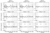 |
Fig. 5. Energetic neutral atom flux change rates (between two adjacent CRs) at 0.7 keV, 1.1 keV, and 10 keV over solar cycles 22–24. From left to right, each column indicates Models 1–3, and each row, from top to bottom, indicates the energy 0.7, 1.1, and 10 keV of each model. The shaded regions are intended to distinguish each solar cycle. |
For a thorough examination, we present the rates of change in ENA flux between adjacent CR times (in percent) over the entire energy range of 0.1–50 keV for solar cycles 22, 23, and 24 in Figs. 6, A.1, and A.2, respectively. The lower three panels in each figure display results for the three ion models. A few key features are noteworthy. First, in Model 1 and 2, as shown in all three figures, a notable flux change – reaching up to a few tens of percent near 1 keV or lower – stands out compared to those at other energies. This feature is absent in Model 3. As demonstrated earlier, this phenomenon is attributed to the sensitive variations in the cutoff energy of the filled-shell distribution used in Models 1 and 2, which responds to the fluctuations in solar wind bulk speed.
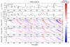 |
Fig. 6. Energetic neutral atom flux change rates (between two adjacent CR times) over the energy range of 0.1–50 keV shown for the IHS ion Models 1, 2, and 3 ((c), (d) and (e), respectively) in response to the solar wind and density variations ((a) and (b)) for solar cycle 22. |
Second, an energy-time dispersion effect is observed in flux response to presumably the same solar wind variations. The response occurs more promptly at higher energies, while lower energy responses exhibit a longer delay time. This time delay effect is due to the energy-dependent retarded time as illustrated in Sect. 2
Lastly, fast temporal variations are predominant during solar cycle 22 across wide energy ranges for all three ion models (see Fig. 6). These variations gradually diminish during solar cycle 23 (Fig. A.1) and 24 (Fig. A.2), aligning with the observed decrease in solar activity.
To effectively examine the correlation between variations in ENA flux and concurrent fluctuations in upstream solar wind parameters – namely speed, density, and dynamic pressure (as shown in the upper two panels of Figs. 6, A.1, and A.2 – we focus on three representative energies: 1.7, 10, and 50 keV. In Fig. 7, ENA fluxes at these energies, normalized to their initial values at CR 1835 (1990-10-25 15:49 UT to 1990-11-21 23:08 UT), are compared against the three solar wind parameters.
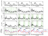 |
Fig. 7. Comparison of the solar wind density (nus), bulk speed (ub, us), and dynamic pressure (Pdyn) upstream of the termination shock with the calculated ENA fluxes observed at 1 AU for three selected ENA energies. The comparison covers three ion models over a 2.5 solar cycle period. The ENA fluxes shown in the bottom panels are normalized to their values at the initial time, CR 1835 (1990-10-25 15:49 UT to 1990-11-21 23:08 UT), separately for each energy. The time [year] axis for the ENA fluxes in the bottom panels refers to the observation time at 1 AU, taking into account the time delay effect illustrated in Sect. 2, whereas the time [year] axis for the sunspot number in the top panels refers to the original time. The highlights in panels (b) and (e) indicate several major increases in number density, which align well with corresponding changes in ENA flux in Model 1. The three intervals highlighted and numbered in panels (h), (i), (m), and (n) correspond to fast solar wind and enhanced dynamic pressure conditions, which show good agreement with the 50 keV ENA flux responses in Models 2 and 3 shown in (j) and (o), respectively. |
First, based on visual inspection of panels (b) and (e) in Fig. 7 (results from Model 1), we find a strong correlation between ENA flux variations and upstream solar wind density. Major increases in number density, highlighted in the figure for clarity, align well with corresponding changes in ENA flux. It is important to note that Model 1 does not include reflected PUIs. In contrast, Model 2 and 3, which include reflected PUIs, exhibit distinctly different behavior, particularly at 50 keV (red curve), where PUIs dominate the high-energy regime. We identify three instances exhibiting these differences, marked with arrows and numbers in panels (j) and (o).
Similarly, in Model 1 (panel (e)) without reflected PUIs, there is no clear correlation between ENA flux changes and upstream bulk speed (panel (c)) at any of the three energies. However, in Models 2 and 3 (panels (j) and (o)), which include reflected PUIs, the 50 keV ENA fluxes show a strong correlation with the bulk speed. We highlight three intervals of fast solar wind, likely corresponding to coronal hole high-speed streams during the declining phases of each of the three solar cycles. The high-energy ENA flux responses during these intervals are both significant and prompt, with minimal time delay. Similar behavior appears in the upstream dynamic pressure (panels (i) and (n)). This resemblance to the bulk speed case is expected, as the dynamic pressure during fast solar wind streams is predominantly governed by the bulk speed.
4. Summary and discussion
In summary, this study investigated the sensitivity of ENAs to solar wind changes at CR resolution, considering three ion distribution models in the IHS. We found that ENA fluxes can exhibit substantial change between adjacent CRs, often correlating with fluctuations in the solar wind speed (primarily at higher energies (> ∼ 10 keV) and density (at lower energies) upstream of the termination shock. The details of these ENA changes depend on the ion distribution model and energy. Notably, employing a filled-shell distribution for transmitted pickup ions induces significant alterations in ENA flux near their cutoff energy, highlighting the importance of precise pickup ion information for accurate ENA estimation during fast changes of the solar wind. Additionally, the inclusion of reflected PUIs is crucial in the high-energy regime (> ∼ 10 keV), where the ENA fluxes exhibit strong correlations with variations in solar wind bulk speed and dynamic pressure.
The correlation between the solar wind at 1 AU and the ion responses in the IHS necessitates consideration of the transit time for the solar wind parcel of each CR number from 1 AU to the TS. In this study, we employed a reduction effect for the solar wind speed and density according to the model by Lee et al. (2009), as illustrated in Sect. 2.2. We acknowledge that this approach may not be entirely realistic due to some inherent limitations. Firstly, the reduction of solar wind speed in radial distance in Lee et al. (2009) is determined by a simple expression derived from the time-stationary solution of purely gas dynamics equations, which does not precisely capture the actual conditions reflecting time-varying solar wind dynamics. In addition, temporal changes in solar EUV impact solar wind speed as well, thus affecting transit times to the TS and the solar wind’s structure near the TS (Bzowski et al. 2013; Lee et al. 2009; Swaczyna et al. 2016). Consequently, changes in the solar wind speed with the radial distance and the subsequent estimation of transit times from 1 AU to TS pose a nontrivial problem.
The main results in Sect. 3 are based on the assumption in Sect. 2 that the thickness of the IHS is 30 AU, which remains constant over time. However, it can vary with time due to some factors such as solar wind density, speed or cosmic rays, which are influenced by the solar cycle (Whang & Burlanga 1993; Zank 1999; Zank & Müller 2003; Washimi et al. 2007; Manuel et al. 2015; Izmodenov & Alexashov 2020). To account for this variability, we repeated the same analysis as in Sect. 2 using thickness values of 25 AU and 35 AU, considering these values as representing a reasonable range for minimum and maximum variations. Our findings indicate that, overall, as the IHS thickness increases, there is a weak tendency for the ENA flux to become larger mostly within a few percentage points. Additionally, we find that the temporal change rates of ENA fluxes across adjacent CRs are mostly insensitive to variations in IHS thickness. Mostly, the temporal change rates of ENA fluxes across adjacent CRs differ by within a few percentage points between the cases of 30 AU and either 25 AU or 35 AU although we do not present details here. Therefore, it implies that the main results in Sect. 3 are not significantly influenced by the temporal variations of the IHS thickness within the 25–35 AU range.
In our current investigation, we have made the simplifying assumption that the form and conditions of IHS ion distributions vary only due to the decreasing density and temperature with increasing distance from the TS. However, we acknowledge that this simplification does not capture the realistic complexity of the IHS environment. Beyond the convection effects within the IHS, ions are likely subjected to various dynamic phenomena, including waves, shocks, instabilities, turbulences, and structures such as the globally merged interaction region, which may be transmitted from upstream or reflected from the heliopause (Richardson et al. 2023). Each of these mechanisms that can affect evolution of ion distributions requires a comprehensive study, which is beyond the scope of the present study.
In our current study, our focus has been directed exclusively toward the noseward direction on the equatorial region. Expanding our investigation to explore ion responses in the off-equatorial IHS region under rapidly varying solar wind conditions is a logical extension. This can be achieved by employing a solar wind model with latitudinal dependence and CR time resolution, as suggested by Sokół et al. (2015). However, it is essential to recognize that the IHS thickness increases away from the equator, resulting in a larger spatial extent of the ENA-originating layer compared to the equatorial plane (Reisenfeld et al. 2016). Our approach to ENA flux integration becomes less accurate in this context. The increased spatial dimensions of the ENA-originating layer suggest that the direct impact of temporal variations in the pre-TS solar wind may be limited radially across the IHS. Instead, as discussed in the previous paragraph, indirect effects such as waves, shocks, and turbulence generated at the TS and within the IHS might emerge as dominant factors influencing ion distributions. It is crucial to consider that, at any given time, different latitudinal portions of the TS experience distinct solar wind structures. Moreover, within a specific latitude, IHS ions intersecting the line of sight (LOS) to an observing satellite (e.g., IBEX) follow diverse travel histories along different streamlines. These streamlines enter the heliosheath at various latitudes, exposing the ions to differing conditions in terms of waves, shocks, turbulence, charge exchange, and variable travel times during their convection along streamlines. The complexity introduced by these factors makes the assessment of off-equatorial ion responses to rapidly varying solar wind highly intricate. A quantitative understanding becomes imperative to determine the extent to which IHS ions respond directly to rapidly changing solar wind conditions and the potentially cumulative effects on IHS ions due to various processes and structures within the IHS itself. This undertaking represents a key task in advancing our comprehension of the intricate dynamics in the off-equatorial IHS region.
Even with a theoretical understanding of the IHS ion responses to rapid variations in solar wind and the continuous observation of the resulting ENA fluxes with the high time resolution, there are limitations imposed by the finite energy resolution (ΔE/E) of ENA sensors (Reisenfeld et al. 2012, 2016; Schwadron & Bzowski 2018; Schwadron et al. 2018). The energy resolution of ENA sensors significantly influences the ability to resolve fast-varying ENA fluxes. For instance, the IBEX-Hi sensor exhibits a large energy resolution (ΔE/E ∼ 65%), leading to notable time dispersion in the observation of ENAs originating beyond the TS (Reisenfeld et al. 2012). The future ENA sensor on board the IMAP spacecraft is anticipated to feature an improved energy resolution (McComas et al. 2018), rendering it more suitable for effectively resolving fast-varying ENA fluxes. This enhanced capability is crucial for advancing our ability to discern finer details in the dynamic processes occurring in the IHS, providing a more accurate representation of the temporal variations in ENA fluxes associated with solar wind dynamics.
Acknowledgments
This work was supported by the National Research Foundation of Korea (NRF) grant funded by the Korea government (MSIT) (RS-2024-00454886). This work was also supported by the National Research Foundation of Korea (NRF) grant funded by the Korea government (MSIT), NRF-2020R1A2C1013159. This work was also supported by basic research funding from Korea Astronomy and Space Science Institute, Korea Aerospace Administration (KASA), and the Institute of Information and Communications Technology Planning and Evaluation (IITP) (MSIT; No. RS-2023-00235534, Near-Earth ≳10 MeV Solar Proton Event Prediction by probing into Solar Wind Condition with Automatic CME detection).
References
- Abramowitz, M., & Stegun, I. A. 1970, Handbook of Mathematical Functions : With Formulas, Graphs, and Mathematical Tables (Washington, D.C.: U.S. Dept. of Commerce, National Bureau of Standards) [Google Scholar]
- Bera, R. K., Fraternale, F., Pogorelov, N. V., et al. 2023, ApJ, 954, 147 [Google Scholar]
- Burgess, D. 1995, in Introduction to Space Physics, eds. M. G. Kivelson, & C. T. Russell (Cambridge University Press), 129, chapter 5 in Kivelson and Russell (eds.) [CrossRef] [Google Scholar]
- Burlaga, L. 2015, J. Phys. Conf. Ser., 642, 012003 [Google Scholar]
- Bzowski, M., Möbius, E., Tarnopolski, S., Izmodenov, V., & Gloeckler, G. 2009, Space Sci. Rev., 143, 177 [Google Scholar]
- Bzowski, M., Sokół, J. M., Tokumaru, M., et al. 2013, in Cross-Calibration of Far UV Spectra of Solar System Objects and the Heliosphere, eds. E. Quémerais, M. Snow, & R.-M. Bonnet, 13, 67 [Google Scholar]
- Dialynas, K., Krimigis, S. M., Mitchell, D. G., Roelof, E. C., & Decker, R. B. 2013, ApJ, 778, 40 [NASA ADS] [CrossRef] [Google Scholar]
- Fahr, H.-J., & Scherer, K. 2004, Astrophys. Space Sci. Trans., 1, 3 [Google Scholar]
- Fahr, H. J., Siewert, M., McComas, D. J., & Schwadron, N. A. 2011, A&A, 531, A77 [NASA ADS] [CrossRef] [EDP Sciences] [Google Scholar]
- Funsten, H. O., Allegrini, F., Crew, G. B., et al. 2009, Science, 326, 964 [NASA ADS] [CrossRef] [Google Scholar]
- Gamayunov, K. V., Zhang, M., Pogorelov, N. V., Heerikhuisen, J., & Rassoul, H. K. 2012, ApJ, 757, 74 [Google Scholar]
- Gamayunov, K. V., Heerikhuisen, J., & Rassoul, H. 2017, ApJ, 845, 63 [Google Scholar]
- Geiss, J., Gloeckler, G., Mall, U., et al. 1994, A&A, 282, 924 [NASA ADS] [Google Scholar]
- Gloeckler, G., Fisk, L. A., & Geiss, J. 1997, Nature, 386, 374 [Google Scholar]
- Gloeckler, G., Möbius, E., Geiss, J., et al. 2004, A&A, 426, 845 [NASA ADS] [CrossRef] [EDP Sciences] [Google Scholar]
- Gruntman, M., Roelof, E. C., Mitchell, D. G., et al. 2001, J. Geophys. Res., 106, 15767 [Google Scholar]
- Heerikhuisen, J., Pogorelov, N. V., Zank, G. P., & Florinski, V. 2007, ApJ, 655, L53 [Google Scholar]
- Heerikhuisen, J., Pogorelov, N. V., Florinski, V., Zank, G. P., & le Roux, J. A. 2008, ApJ, 682, 679 [NASA ADS] [CrossRef] [Google Scholar]
- Heerikhuisen, J., Zirnstein, E. J., Funsten, H. O., Pogorelov, N. V., & Zank, G. P. 2014, ApJ, 784, 73 [Google Scholar]
- Heerikhuisen, J., Zirnstein, E. J., Pogorelov, N. V., Zank, G. P., & Desai, M. 2019, ApJ, 874, 76 [Google Scholar]
- Izmodenov, V. V., & Alexashov, D. B. 2020, A&A, 633, L12 [NASA ADS] [CrossRef] [EDP Sciences] [Google Scholar]
- Izmodenov, V. V., Malama, Y. G., Ruderman, M. S., et al. 2009, Space Sci. Rev., 146, 329 [Google Scholar]
- Kornbleuth, M., Opher, M., Michael, A. T., & Drake, J. F. 2018, ApJ, 865, 84 [Google Scholar]
- Krimigis, S. M., Mitchell, D. G., Roelof, E. C., Hsieh, K. C., & McComas, D. J. 2009, Science, 326, 971 [NASA ADS] [CrossRef] [Google Scholar]
- Lazar, M., & Fichtner, H. 2021, in Kappa Distributions; From Observational Evidences via Controversial Predictions to a Consistent Theory of Nonequilibrium Plasmas, eds. M. Lazar, & H. Fichtner, Astrophys. Space Sci. Lib., 464, 321 [Google Scholar]
- Lazarus, A. J., & McNutt, R. L., J. 1990, in Physics of the Outer Heliosphere, eds. S. Grzedzielski, & D. E. Page, 229 [Google Scholar]
- Lee, M. A., Fahr, H. J., Kucharek, H., et al. 2009, Space Sci. Rev., 146, 275 [Google Scholar]
- Lindsay, B. G., & Stebbings, R. F. 2005, J. Geophys. Res.: Space Phys., 110, A12213 [Google Scholar]
- Livadiotis, G., McComas, D. J., Dayeh, M. A., Funsten, H. O., & Schwadron, N. A. 2011, ApJ, 734, 1 [NASA ADS] [CrossRef] [Google Scholar]
- Livadiotis, G., McComas, D. J., Randol, B. M., et al. 2012, ApJ, 751, 64 [NASA ADS] [CrossRef] [Google Scholar]
- Livadiotis, G., Desai, M. I., & Wilson, L. B., I. 2018, ApJ, 853, 142 [Google Scholar]
- Manuel, R., Ferreira, S. E. S., & Potgieter, M. S. 2015, ApJ, 799, 223 [NASA ADS] [CrossRef] [Google Scholar]
- McComas, D. J., Allegrini, F., Bochsler, P., et al. 2009, Science, 326, 959 [NASA ADS] [CrossRef] [Google Scholar]
- McComas, D. J., Zirnstein, E. J., Bzowski, M., et al. 2017a, ApJS, 233, 8 [NASA ADS] [CrossRef] [Google Scholar]
- McComas, D. J., Zirnstein, E. J., Bzowski, M., et al. 2017b, ApJS, 229, 41 [Google Scholar]
- McComas, D. J., Christian, E. R., Schwadron, N. A., et al. 2018, Space Sci. Rev., 214, 116 [CrossRef] [Google Scholar]
- McComas, D. J., Bzowski, M., Dayeh, M. A., et al. 2020, ApJS, 248, 26 [Google Scholar]
- McComas, D. J., Swaczyna, P., Szalay, J. R., et al. 2021, ApJS, 254, 19 [Google Scholar]
- McComas, D. J., Shrestha, B. L., Swaczyna, P., et al. 2022, ApJ, 934, 147 [Google Scholar]
- Möbius, E., Hovestadt, D., Klecker, B., et al. 1985, Nature, 318, 426 [Google Scholar]
- Möbius, E., Liu, K., Funsten, H., Gary, S. P., & Winske, D. 2013, ApJ, 766, 129 [Google Scholar]
- Pierrard, V., & Lazar, M. 2010, Sol. Phys., 267, 153 [NASA ADS] [CrossRef] [Google Scholar]
- Prested, C., Schwadron, N., Passuite, J., et al. 2008, J. Geophys. Res.: Space Phys., 113, A06102 [Google Scholar]
- Randol, B. M., McComas, D. J., & Schwadron, N. A. 2013, ApJ, 768, 120 [Google Scholar]
- Reisenfeld, D. B., Allegrini, F., Bzowski, M., et al. 2012, ApJ, 747, 110 [Google Scholar]
- Reisenfeld, D. B., Bzowski, M., Funsten, H. O., et al. 2016, ApJ, 833, 277 [NASA ADS] [CrossRef] [Google Scholar]
- Richardson, J. D. 1997, Geophys. Res. Lett., 24, 2889 [Google Scholar]
- Richardson, J. D., Kasper, J. C., Wang, C., Belcher, J. W., & Lazarus, A. J. 2008, Nature, 454, 63 [NASA ADS] [CrossRef] [Google Scholar]
- Richardson, J. D., Bykov, A., Effenberger, F., et al. 2023, Space Sci. Rev., 219, 6 [NASA ADS] [CrossRef] [Google Scholar]
- Scherer, K., & Fahr, H. J. 2003a, Ann. Geophys., 21, 1303 [Google Scholar]
- Scherer, K., & Fahr, H. J. 2003b, Geophys. Res. Lett., 30, 1045 [NASA ADS] [CrossRef] [Google Scholar]
- Scherer, K., Fichtner, H., & Lazar, M. 2017, Europhys. Lett., 120, 50002 [NASA ADS] [CrossRef] [Google Scholar]
- Scherer, K., Fichtner, H., Fahr, H. J., & Lazar, M. 2019, ApJ, 881, 93 [NASA ADS] [CrossRef] [Google Scholar]
- Scherer, K., Dialynas, K., Fichtner, H., Galli, A., & Roussos, E. 2022, A&A, 664, A132 [NASA ADS] [CrossRef] [EDP Sciences] [Google Scholar]
- Schwadron, N. A., & Bzowski, M. 2018, ApJ, 862, 11 [Google Scholar]
- Schwadron, N. A., & McComas, D. J. 2013, ApJ, 764, 92 [NASA ADS] [CrossRef] [Google Scholar]
- Schwadron, N. A., & McComas, D. J. 2019, ApJ, 887, 247 [CrossRef] [Google Scholar]
- Schwadron, N. A., Allegrini, F., Bzowski, M., et al. 2011, ApJ, 731, 56 [NASA ADS] [CrossRef] [Google Scholar]
- Schwadron, N. A., Allegrini, F., Bzowski, M., et al. 2018, ApJS, 239, 1 [Google Scholar]
- Shrestha, B. L., Zirnstein, E. J., Heerikhuisen, J., & Zank, G. P. 2021, ApJS, 254, 32 [Google Scholar]
- Siewert, M., Fahr, H. J., McComas, D. J., & Schwadron, N. A. 2012, A&A, 539, A75 [NASA ADS] [CrossRef] [EDP Sciences] [Google Scholar]
- Sokół, J. M., Swaczyna, P., Bzowski, M., & Tokumaru, M. 2015, Sol. Phys., 290, 2589 [Google Scholar]
- Sokół, J. M., McComas, D. J., Bzowski, M., & Tokumaru, M. 2020, ApJ, 897, 179 [Google Scholar]
- Stone, E. C., Cummings, A. C., McDonald, F. B., et al. 2005, Science, 309, 2017 [NASA ADS] [CrossRef] [Google Scholar]
- Swaczyna, P., Bzowski, M., & Sokół, J. M. 2016, ApJ, 827, 71 [Google Scholar]
- Vasyliunas, V. M. 1968, in Physics of the Magnetosphere, eds. R. D. L. Carovillano, & J. F. McClay, Astrophys. Space Sci. Lib., 10, 622 [NASA ADS] [CrossRef] [Google Scholar]
- Vasyliunas, V. M., & Siscoe, G. L. 1976, J. Geophys. Res., 81, 1247 [NASA ADS] [CrossRef] [Google Scholar]
- Washimi, H., Zank, G. P., Hu, Q., Tanaka, T., & Munakata, K. 2007, ApJ, 670, L139 [Google Scholar]
- Whang, Y. C., & Burlanga, L. F. 1993, J. Geophys. Res., 98, 15221 [Google Scholar]
- Zank, G. P. 1999, Space Sci. Rev., 89, 413 [NASA ADS] [CrossRef] [Google Scholar]
- Zank, G. P., & Müller, H. R. 2003, J. Geophys. Res.: Space Phys., 108, 1240 [Google Scholar]
- Zank, G. P., Heerikhuisen, J., Pogorelov, N. V., Burrows, R., & McComas, D. 2010, ApJ, 708, 1092 [NASA ADS] [CrossRef] [Google Scholar]
- Zirnstein, E. J., Heerikhuisen, J., Zank, G. P., et al. 2014, ApJ, 783, 129 [Google Scholar]
- Zirnstein, E. J., Heerikhuisen, J., Pogorelov, N. V., McComas, D. J., & Dayeh, M. A. 2015, ApJ, 804, 5 [Google Scholar]
Appendix A: The ENA flux change rates between adjacent CR times
Here we present the ENA flux change rates between adjacent CR times (in percent) over the entire energy range of 0.1–50 keV for solar cycles 23 and 24, as an extension of Fig. 6 corresponding to solar cycle 22.
All Tables
All Figures
|
Fig. 1. (Upper panel) Schematic illustration of the core concept behind the interaction between solar radiation, solar wind protons, and interstellar neutrals leading to the formation of pickup ions through ionization and/or charge exchange in the supersonic solar wind. Pickup ions are tied to the heliospheric magnetic field and are transported outward by the solar wind. These processes generate energetic neutral atoms via charge exchange between solar wind protons, pickup ions, and interstellar neutrals in the inner heliosheath – the region between the termination shock and the heliopause. The outer heliosheath is the region in the very local interstellar medium adjacent to the heliopause. (Lower panels) Overview of the current understanding of ion distributions in the inner heliosheath, the availability of bulk solar wind data, and a flowchart summarizing the main ideas of the study. |
| In the text | |
|
Fig. 2. (a) Sunspot number. (b) Solar wind speed and (c) Solar wind density at 1 AU (black) and 90 AU (pink) at a time resolution of Carrington rotation. In (b) and (c), the data at 1 AU are available from OMNI data center, while those at 90 AU were obtained by considering differing transit times of solar wind parcels of different CRs using the simplified model of Lee et al. (2009). Accordingly, the solar wind profile at 90 AU (pink) begins about one year later than the profile at 1 AU (black). (For more details, see the first two paragraphs of Sect. 2.2). |
| In the text | |
|
Fig. 3. (a) Solar wind bulk speed in the upstream of the termination shock. This is in fact the same data as the solar wind speed at 90 AU shown in Fig. 2b, repeated for convenience. (b) Compression ratio R defined by Eq. (10). (c) Cutoff energy of filled-shell distribution defined by Eq. (9). (d) Temperature of reflected PUI distribution defined by Eq. (7). (e) PUI density ratio relative to total ion density in the inner heliosheath, that is, |
| In the text | |
|
Fig. 4. Variation of ENA fluxes at Carrington rotation time resolution across solar cycles 22, 23, and 24, with colored lines representing different ENA energies. The time on the horizontal axis refers to the observation time at 1 AU. Models 1, 2, and 3 from left to right refer to the results for three ion distribution models in the inner heliosheath. |
| In the text | |
|
Fig. 5. Energetic neutral atom flux change rates (between two adjacent CRs) at 0.7 keV, 1.1 keV, and 10 keV over solar cycles 22–24. From left to right, each column indicates Models 1–3, and each row, from top to bottom, indicates the energy 0.7, 1.1, and 10 keV of each model. The shaded regions are intended to distinguish each solar cycle. |
| In the text | |
|
Fig. 6. Energetic neutral atom flux change rates (between two adjacent CR times) over the energy range of 0.1–50 keV shown for the IHS ion Models 1, 2, and 3 ((c), (d) and (e), respectively) in response to the solar wind and density variations ((a) and (b)) for solar cycle 22. |
| In the text | |
|
Fig. 7. Comparison of the solar wind density (nus), bulk speed (ub, us), and dynamic pressure (Pdyn) upstream of the termination shock with the calculated ENA fluxes observed at 1 AU for three selected ENA energies. The comparison covers three ion models over a 2.5 solar cycle period. The ENA fluxes shown in the bottom panels are normalized to their values at the initial time, CR 1835 (1990-10-25 15:49 UT to 1990-11-21 23:08 UT), separately for each energy. The time [year] axis for the ENA fluxes in the bottom panels refers to the observation time at 1 AU, taking into account the time delay effect illustrated in Sect. 2, whereas the time [year] axis for the sunspot number in the top panels refers to the original time. The highlights in panels (b) and (e) indicate several major increases in number density, which align well with corresponding changes in ENA flux in Model 1. The three intervals highlighted and numbered in panels (h), (i), (m), and (n) correspond to fast solar wind and enhanced dynamic pressure conditions, which show good agreement with the 50 keV ENA flux responses in Models 2 and 3 shown in (j) and (o), respectively. |
| In the text | |
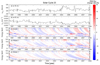 |
Fig. A.1. Same as for Fig. 6 but for solar cycle 23. |
| In the text | |
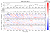 |
Fig. A.2. Same as for Fig. 6 but for solar cycle 24. |
| In the text | |
Current usage metrics show cumulative count of Article Views (full-text article views including HTML views, PDF and ePub downloads, according to the available data) and Abstracts Views on Vision4Press platform.
Data correspond to usage on the plateform after 2015. The current usage metrics is available 48-96 hours after online publication and is updated daily on week days.
Initial download of the metrics may take a while.