| Issue |
A&A
Volume 699, July 2025
|
|
|---|---|---|
| Article Number | A329 | |
| Number of page(s) | 18 | |
| Section | Extragalactic astronomy | |
| DOI | https://doi.org/10.1051/0004-6361/202451713 | |
| Published online | 23 July 2025 | |
Are compact groups of galaxies special?
1
17, rue des plantes, 75014 Paris, France
2
Institut d’Astrophysique de Paris (UMR 7095: CNRS & Sorbonne Université), 98 bis boulevard Arago, 75014 Paris, France
3
CONICET. Instituto de Astronomía Teórica y Experimental (IATE), Laprida 854, X5000BGR Córdoba, Argentina
4
Universidad Nacional de Córdoba (UNC). Observatorio Astronómico de Córdoba (OAC), Laprida 854, X5000BGR Córdoba, Argentina
⋆ Corresponding author: This email address is being protected from spambots. You need JavaScript enabled to view it.
Received:
29
July
2024
Accepted:
23
April
2025
Abstract
It is often believed that isolated compact groups (CGs) of galaxies are special systems, but only a few studies have compared CGs to regular groups. We study the global properties and internal correlations of a volume- and luminosity-complete subsample of 78 groups of four members (CG4s) within the HMCG Hickson-like sample of compact groups. We compared these CGs to those of a similarly built subsample (including the three-magnitude range of CG4s) of the Lim regular groups. The latter were split into three control samples: one with the four brightest members (Control4Bs), one with the four closest members to the brightest group galaxy (BGG; Control4Cs), and one with exactly four members (RG4s). The vast majority of the CG4s are located within regular groups, and a large preponderance of the BGGs of these CG4s are the same as those of their host groups. The CG4s are smaller than the groups of all other samples and more luminous than RG4s. Both results are a consequence of their selection as high surface brightness systems. However, the CG4s (especially those split among several regular groups) have luminosities similar to Control4Cs. The CG4s also have higher velocity dispersions, probably because of a too-permissive redshift accordance criterion. The BGGs of the CG4s are not any more dominant in luminosity than those of RG4s, but they are significantly more offset relative to the group size because the Lim groups are built around their BGGs. In summary, compact groups have similar properties to regular groups of four galaxies and to the cores of regular groups once the selection criteria of CGs are considered. A large fraction of the CGs are the cores of regular groups, which are isolated on the sky by construction but rarely isolated in real space (from simulations), indicating that they are often plagued by chance alignments of host group galaxies along the line of sight.
Key words: catalogs / galaxies: clusters: general
© The Authors 2025
 Open Access article, published by EDP Sciences, under the terms of the Creative Commons Attribution License (https://creativecommons.org/licenses/by/4.0), which permits unrestricted use, distribution, and reproduction in any medium, provided the original work is properly cited.
This article is published in open access under the Subscribe to Open model. This email address is being protected from spambots. You need JavaScript enabled to view it. to support open access publication.
1. Introduction
Isolated compact groups (CGs) of four or more galaxies of comparable luminosity, though fairly rare, constitute a potentially extremely dense environment that serves as a unique laboratory to study galaxy interactions. The natural point of view is that CGs constitute physically dense systems (Hickson & Rood 1988). But many authors have challenged this view by suggesting that CGs are unbound (Burbidge & Burbidge 1961), transient (Rose 1977 for elongated CGs), or mainly contaminated by chance alignments of galaxies along the line of sight (Mamon 1986; Walke & Mamon 1989). Semi-analytical models (SAMs) of galaxy formation have been used to test the chance alignment hypothesis, starting with the works of McConnachie et al. (2008) and Díaz-Giménez & Mamon (2010). The latest, (Díaz-Giménez et al. 2020), indicates that roughly half of Hickson-like samples in SAMs are indeed chance alignments. This fraction is higher for a greater cosmological density parameter, Ωm, and for a lower amplitude of the power spectrum of primordial density fluctuations, σ8, but is also lower with higher resolution of the parent dark matter only cosmological simulation on which the SAM was run.
If CGs are indeed extremely dense non-transient environments, one may wonder whether their global properties differ from those of other groups. This question is best answered with well-defined catalogs of CGs. The most popular of such catalogs was assembled by Hickson (1982), who first searched on photographic plates for isolated compact groups of at least four galaxies within a three-magnitude range. His compactness criterion was based on mean surface brightness, and it led to the HCG catalog of exactly 100 groups. Later, a spectroscopic follow-up (Hickson et al. 1992) indicated that 69 of the groups contained at least four galaxies of concordant redshifts. The HCG catalog suffers from not only its small size but also from biases. The most important of these biases is the one against CGs dominated by a single galaxy (but still satisfying the three-magnitude range), as found from automatic CG selection from photographic plates (Prandoni et al. 1994) and from expectations from semi-analytical models (Díaz-Giménez & Mamon 2010).
Several catalogs of CGs have been produced by automatic selection, most with highly incomplete photometric or spectroscopic data. The notable exceptions are those extracted from the Two Micron All-Sky Survey (2MASS) Redshift Survey (i.e., Díaz-Giménez et al. 2012) and from the Sloan Digital Sky Survey (SDSS; i.e, McConnachie et al. 2009; Sohn et al. 2015, 2016; Díaz-Giménez et al. 2018; Zheng & Shen 2020; Zandivarez et al. 2022). While McConnachie et al. (2009) managed to produce two large catalogs of CGs (with nearly 2300 and 75 000 groups), only two CGs within them had complete redshift coverage and satisfied the HCG criteria of surface brightness and accordant redshifts (Díaz-Giménez et al. 2018). Similarly, the catalogs of Sohn et al. (2015, 2016) contain 300 and nearly 1600 CGs, among which only 11 and 142 respectively meet the HCG criteria.
One of the largest catalogs of HCGs with complete spectroscopy and meeting the HCG criteria is the Hickson Modified Compact Group (HMCG) sample of Díaz-Giménez et al. (2018), who extracted groups from the SDSS Main Galaxy Sample, yielding 406 CGs with good flags. Díaz-Giménez et al. (2018) obtained this large sample by performing their CG selection in one step instead of the original two-phase selection (i.e., first photometric, then spectroscopic). Indeed, photometric selection discards groups that seem not to be isolated, whereas their neighbors are often later found to have discordant redshifts and are thus unrelated. Zheng & Shen (2020) built a sample (“cCG”) of 6144 CGs of at least three members that meet the HCG criteria and have complete redshift information. Their cCG sample is mainly based on the SDSS Main Galaxy Sample, but it is supplemented with redshifts from the Large sky Area Multi-Object fiber Spectroscopic Telescope (LAMOST) (Luo et al. 2015) and the Galaxy Mass Assembly (GAMA) (Liske et al. 2015) surveys, and as well as from other sources. It contains 847 groups of over four galaxies and 698 groups with exactly four galaxies. It is the largest compact group sample with complete redshift information. However, the Zheng & Shen (2020) catalog includes groups with magnitude ranges greater than three magnitudes as well as many more groups with too-faint brightest galaxy magnitudes to allow for a possible range of three magnitudes, which is important for studying luminosity functions and magnitude gaps. Their sample contains only 135 groups of four galaxies with an SDSS red magnitude rbright≤14.77, while none have more than four members. Finally, Zandivarez et al. (2022) produced a catalog with 1412 CGs of at least three members, but it contains only 300 CGs with four or more galaxies.
A fundamental question concerning CGs is how their properties compare to those of “regular” groups. This comparison was unfeasible until group catalogs were built with overdensities roughly matching the “virial” criterion for dynamical equilibrium (overdensities relative to the critical density, 3H2/(8π G), on the order of 100 in the low-redshift Universe). An example of this type of catalog is the popular Yang et al. (2007) group catalog. Using a SAM, Zandivarez et al. (2014) found no difference in the size and shape of CGs compared to those of regular groups with similar projected separation between the first- and second-ranked galaxies. On the other hand, Zandivarez et al. (2022) have claimed a slight but significant deficiency of faint (Mr>−17) galaxies in CGs compared to regular groups.
The properties of a CG also depend on its position relative to its host group. Díaz-Giménez & Zandivarez (2015) found that CGs embedded in regular groups have smaller sizes and a higher surface brightness than non-embedded CGs. More recently, Zheng & Shen (2021) found that roughly half of their CGs are embedded in regular groups, whereas roughly one quarter are “Isolated” compact groups, leaving almost another quarter of their compact groups “Split” between several regular groups. They also found that over half of the embedded CGs dominate the luminosity of the parent group. They call these “Predominant”, while those not dominating the group luminosity are called “Embedded” and have higher velocity dispersions than both the Isolated CGs and non-compact groups (which have similar velocity dispersions as the Isolated CGs)1.
This article aims to go beyond the pioneering analysis of Zheng & Shen (2021) by addressing the following points: 1) determining how the relative populations of classes of CGs defined by Zheng & Shen (2021) differ when only considering compact groups of at least four galaxies (of concordant luminosities), to better conform with the original intent of Hickson (1982); (2) finding out where the embedded CGs (i.e., in both Predominant and Embedded classes) are located relative to their parent groups; 3) studying how the CG properties and their correlations compare to those of previous catalogs.
To answer these questions, we adopted the CG catalog of Díaz-Giménez et al. (2018), which as mentioned above is the largest fully complete sample of CGs in magnitude range and available spectroscopy. More precisely, we considered the majority of the CGs that have exactly four member galaxies. We compare the compact groups to control samples formed from the regular group catalog of Lim et al. (2017). When comparing CG and regular group samples, one should note that Lim et al. (2017) and Díaz-Giménez et al. (2018) did not adopt the same algorithms to build their groups, nor did they start from the same set of galaxies. In fact, some HMCGs are split among several (up to four) Lim groups2.
We present the CG data and the control samples in Sect. 2, discuss the locations of CGs relative to regular groups in Sect. 3, and describe the CG structure and fundamental properties in Sect. 4. In Sect. 5, we present and discuss our conclusions.
Throughout this article, following Tempel et al. (2017), we adopt cosmological parameters for a flat Universe with Ωm = 0.308, Neff = 3.15, and h = 0.678 (Planck Collaboration XIII 2016), and all our logarithms are base 10.
2. Data
2.1. Galaxies
We obtained galaxy properties from the Friends-of-Friends group catalog that Tempel et al. (2017) extracted from Data Release 12 of the SDSS Main Galaxy Sample. Tempel et al. made a great effort to remove poorly measured galaxies. Their catalog3 contains 584 449 galaxies up to a redshift of 0.2 in the frame of the cosmic microwave background (CMB).
Absolute magnitudes are derived from apparent magnitudes using distances in the Planck cosmology (Planck Collaboration XIII 2016), Galactic extinction from Schlegel et al. (1998), k-corrections from Blanton & Roweis (2007), and evolutionary corrections from Blanton et al. (2003). Although k+e corrections in Tempel et al. (2017) are not described, it is likely that they follow those in Tempel et al. (2014), which are based on Blanton & Roweis (2007) for k and Blanton et al. (2003) for e, assuming a distance-independent luminosity function. We derived r-band luminosities assuming a solar absolute magnitude of M⊙,r = 4.684. All matching of SDSS-based catalogs shown in Table 1 (see Sect. 2.4) are based on SDSS galaxy OBJID.
Summary of the group samples used in this study.
2.2. Regular groups
We use the group catalog5 identified by Lim et al. (2017) from SDSS DR7, who essentially followed the group-finding algorithm of Yang et al. (2007). The algorithm of Lim et al. (2017) works in the five following steps: 1) it starts by assigning a single-galaxy group to each galaxy; 2) it determines the virial radius and velocity dispersion of each group using the group luminosity - total mass relation determined from a cosmological hydrodynamical simulation; 3) it estimates a “factor” (related to the probability of membership) linking each galaxy to each group; 4) it assigns each galaxy to the group with its highest factor; 5) it iterates from step 2, modified to use abundance matching between group luminosity and the halo mass function measured form cosmological simulations for groups of more than one galaxy. We work with their sample SDSS(L)group.dat that comprises 446 495 groups with one or more members containing 586 025 galaxies. The “L” version means it is constructed with galaxies that have spectroscopic redshifts, using Proxy-L (based on galaxy luminosities) to estimate halo masses. In this sample, 388 819 groups have a single galaxy, while 12 213 have four or more members.
We first removed the twelve duplicate galaxies from the catalog. We then found that 9420 galaxies in these groups do not belong to the Tempel et al. (2017) galaxy catalog. Since we are using galaxy properties from Tempel et al. (2017), we removed from the group catalog 8087 groups that host those galaxies. We are then left with 438 408 groups containing 573 572 galaxies. Hereafter, this restricted sample will be named as Lim-Tempel catalog6.
2.3. Compact groups
2.3.1. Sample
We use the sample of Hickson Modified Compact Groups (HMCG) identified by Díaz-Giménez et al. (2018) on the Tempel et al. (2017) galaxy catalog. The HMCG sample contains 462 compact groups, among which 406 are not flagged as dubious by the authors. By construction, not all the galaxies in HMCG lie in the Tempel et al. (2017) galaxy catalog, because Díaz-Giménez et al. (2018) had added 63 additional galaxies, with redshifts from the NASA Extragalactic Database (see their table B2).
We selected the 284 compact groups among the 406 reliable HMCGs that contain exactly four galaxies. Among these 284 groups, we discarded all those containing at least one galaxy not present in the Lim-Tempel sample, leaving us with 226 compact groups of four galaxies belonging to the Lim-Tempel sample. The reasons for such a high fraction of discarded groups (62/284 = 22%) are the 63 galaxies added by Díaz-Giménez et al. (2018) and the 7000 galaxies added by Tempel et al. (2017) that are not in the SDSS Main Galaxy Sample and the 600 458−586 025 = 14 433 galaxies that are not part of the group catalog of Lim et al. (2017) (field galaxies). Rest-frame absolute magnitudes, CMB redshifts and angular coordinates for galaxies in this subsample are extracted directly from Tempel et al. (2017).
We choose, here, to compare the properties of compact groups and regular groups, controlling for multiplicity (i.e., richness) and galaxy luminosity. We build a subsample of 4-member CGs that is doubly complete in volume and luminosity to prevent selection effects, in particular on the magnitude range, since the Hickson CG multiplicity criterion imposes a minimum of four galaxies within three magnitudes from the BGG, i.e. rBGG<14.77 for our SDSS-based sample. We first required zBGG>0.005 to avoid galaxies whose unknown peculiar velocities will contribute sufficiently to the redshift that the distance inferred from the redshift is too uncertain, leading to too uncertain luminosities. The number of groups in such doubly complete subsamples depends on the choice of maximum redshift or equivalently on minimum luminosity. Starting from the 226 CGs of four galaxies, we recover a maximum of 78 CGs (therefore containing 312 galaxies) for Mr,BGG<−21.81, corresponding to zBGG<0.0452 for rBGG<14.77. This selection is illustrated in Figure 1. We call CG4 this sample of 78 compact groups of four galaxies.
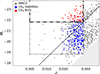 |
Fig. 1. Absolute r-band magnitude versus redshift for galaxies in the HMCG compact group sample and in the CG4 subsample. The colors are gray for all HMCG galaxies, red for CG4 BGGs and blue for CG4 satellites. The shaded gray region represents galaxies fainter than the SDSS flux limit (r>17.77). The dotted line denotes our doubly complete HMCG sample, while the thick dash-dotted lines shows the magnitude and redshift limits for the BGGs. The oblique line is three magnitudes above the SDSS flux limit and is our limit for BGGs in the first-step CG4 selection process. |
2.3.2. Comparison to other compact group samples
We now compare our CG4 catalog to previously published compact group catalogs: Hickson et al. (1992) (HCG)7, McConnachie et al. (2009) (M09)8, Díaz-Giménez et al. (2012) (D12)9, Sohn et al. (2015) (S15)10, Sohn et al. (2016) (S16)11, Zheng & Shen (2020) (Z20)12, Zandivarez et al. (2022) (Z22)13, and Díaz-Giménez et al. (2018) (D18)14.
For a fair comparison, we filtered these catalogs to groups of exactly four redshift-concordant galaxies with our limits in distance (0.005≤zBGG≤0.0452) and luminosity (MBGG≤−21.81), as well as a magnitude concordance criterion (M4−M1≤3). This led to zero M09 groups and only one S15 group, so we discarded both M09 and S15 samples. This left us with 24 compact quartets in HCG, 59 in D12, 31 in S16, 14 in Z20, 88 in Z22, 117 in D18, and 73 in CG415.
We calculated the following group properties for all samples in the same way: median projected galaxy separation 〈Rij〉, group velocity dispersion σv, group luminosity Lgroup, group virial theorem mass ℳVT, relative BGG offset ΔBGG−cen/〈Rij〉, relative BGG velocity offset ΔvBGG/σv, relative BGG luminosity LBGG/Lgroup, magnitude gap M2−M1, crossing time tcr, group virial theorem mass to r-band luminosity ratio ℳVT/Lr.
For the catalogs that only provided observer-frame apparent magnitudes, we used the k-corrections recommended by Chilingarian & Zolotukhin (2012) to obtain rest-frame absolute magnitudes at z = 0 and M⊙ = 4.68. For CG4 we use the rest-frame absolute magnitudes of the galaxy members, Mr, provided by Tempel et al. (2017).
For each group, we converted the angular separations, θi,j, into distances projected on the plane of sky, Ri,j using
 (1)
(1)
where DA(z) is the cosmological angular separation distance16. We computed the line-of-sight velocities of galaxies relative to their group using
 (2)
(2)
The line-of-sight velocity dispersion, σv, was then estimated using the gapper algorithm (Wainer & Thissen 1976), which is the most efficient for measuring radial velocity dispersion for small samples (Beers et al. 1990). Finally, from the rest-frame absolute magnitudes of the galaxy members, we computed the group luminosities from the sum of luminosities of individual galaxies, Lr,group=∑dex[−0.4 (Mr−M⊙)]. Furthermore, the virial theorem mass is (Heisler et al. 1985, written as in Díaz-Giménez et al. 2012)
 (3)
(3)
where  is the harmonic mean projected separation. Following Díaz-Giménez et al. (2012), the crossing time is defined as
 (4)
(4)
where rij are the 3D separations.
The properties of the group samples are compared in the boxplot diagrams of Fig. 217. By construction, the properties of CG4 resemble those of D18, from which it was built (but in the smaller zone covered by Lim et al. 2017). However, the different catalogs were built using different criteria for group compactness and possible isolation. Apart from the samples of Hickson et al. (1992) (HCG) and Sohn et al. (2016) (S16), whose compact quartets are much smaller (their median separations are half those of the other samples), the other samples of compact quartets are in fair agreement with our CG4 sample. Also, the HCG sample shows the smallest magnitude gap and lowest dominance of the BGG. Previous works (Prandoni et al. 1994; Díaz-Giménez & Mamon 2010) had noted that Hickson's visual selection was biased to avoid groups whose magnitude gap is close to the limit of the selection. One other standout sample is that of Zheng & Shen (2020), whose quartets have lower total luminosities and marginally lower relative BGG velocity offsets than those of the other samples.
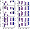 |
Fig. 2. Comparison of CG4 properties with samples of compact quartets built from other published compact group catalogs, with the same selection in redshifts and magnitudes: 0.005≤zBGG≤0.0452, MBGG≤−21.81, and M4−M1≤3. From top left to bottom right, the properties are median of the projected inter-galaxy separations, radial velocity dispersion, total group luminosity, group virial theorem mass, crossing time, mass-to-light ratio, BGG relative offset (normalized distance of the BGG to the centroid of the group), BGG relative velocity offset (normalized distance in radial velocity of the BGG to the group radial velocity dispersion, top-right panel), BGG luminosity fraction, and absolute magnitude difference between the two brightest galaxy members. The abscissa indicate the compact group catalogs: HCG: Hickson et al. (1992), D12: Díaz-Giménez et al. (2012), S16: Sohn et al. (2016), Z20: Zheng & Shen (2020), Z22: Zandivarez et al. (2022), D18: Díaz-Giménez et al. (2018), and CG4: this work. |
2.4. Control samples of regular groups
We built three control samples of regular groups. We began by selecting a subsample of Lim-Tempel groups with the following steps:
-
We discarded all Lim-Tempel groups having their BGG outside of the redshift limits of our CG4 selection (0.005<zBGG<0.0452) to ensure the same level of completeness as for the CG4 groups. This left us with 46 279 groups containing 68 834 galaxies.
-
In this redshift range, we selected groups in the same Mr limits as of our CG4 selection. This yielded 1950 groups (hereafter LTz,Mr), containing 14 265 galaxies, having their BGG brighter than −21.81.
-
We discarded groups with fewer than four galaxies, which led to 1042 groups containing 12 516 galaxies.
-
We retained those groups with at least three satellites whose luminosities lie within 3 absolute magnitudes from their BGG, leaving 765 groups (73% of our previous sample), containing 11 087 galaxies (i.e., an average of 14 galaxies per group). This selection is hereafter named Parent Control catalog (PC). Among 765 PC groups, 68 (9%) contain at least one galaxy from CG4: 57 PC groups have four galaxies from CG4, 5 have three galaxies, 3 have eight, one has six galaxies, one has two and one has a single galaxy. We will discuss in Sect. 3 how CG4s are located within their parent groups.
Figure 3 compares the multiplicity functions of the LTz,Mr (step 2 in Sect. 2.4) and PC (step 4 in Sect. 2.4) groups, in the range 4≤Ngalaxies≤20. LTz,Mr contains roughly one order of magnitude fewer galaxies than Lim-Tempel for multiplicities comprised between 4 and 15. The multiplicity function of RG4 groups is also roughly ten times lower than that of LT groups, and it is even more than ten times lower for groups of fewer than six members.
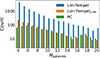 |
Fig. 3. Multiplicity functions of the parent group samples: LT, LTz,Mr (step 2 in Sect. 2.4), and PC (step 4 in Sect. 2.4) in the range 4≤Ngalaxies≤20 (Ngalaxies reaches 538 for PC). The 62 PC groups of four correspond to the RG4 sample. |
From PC groups, we also built three control samples of regular groups of four galaxies:
-
Regular groups of four galaxies (RG4), which comprises 62 groups.
-
Control4B comprise the 765 PCs in which only the BGG and the three other brightest galaxies are selected (the subscript B stands for “brightest”).
-
Control4C is composed of the 765 PCs in which only the BGG and the three closest galaxies to the BGG (in projection) are selected (the subscript C stands for “closest”).
Finally, we excluded the six RG4s whose galaxies are identical to those of a CG4. Thus, six out of 78 CG4s (8%) are a Lim group, and among 62 potential RG4s, 6 (10%) are compact. We also excluded the control groups containing at least one galaxy belonging to a CG4 (66 in Control4B, 61 in Control4C). Our final control samples have 699 groups in Control4B, 704 in Control4C and 56 in RG4. The five group samples used in this study are summarized in Table 1.
The goal of creating control group samples having the same number of galaxies as CG4s is to avoid common multiplicity effects. For example, one can expect that the more galaxies in a group, the more likely there will exist a galaxy having a magnitude closer to the BGG magnitude in this group. Figure 4 shows the relation between absolute magnitude gap and multiplicity for the PC groups. The visual impression is that the gap decreases only weakly with increasing multiplicity. But a Spearman rank test finds a correlation coefficient of –0.2, with a probability of occurring by chance of less than 10−7. Hence, our need to control for multiplicity.
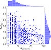 |
Fig. 4. Absolute magnitude difference between the BGG and the second brightest galaxy of each group versus group multiplicity for PC groups. |
3. Location of compact groups within their parent group
3.1. CG4s within groups from the Lim-Tempel catalog and its doubly complete subsample
Since, by construction, the CG4 sample is restricted to compact groups whose members are all members of the Lim-Tempel sample, we can analyze the associations between the two group samples.
Lim-Tempel groups hosting CG4 galaxies have a variety of multiplicities, from a single galaxy to 538 galaxies, with a median multiplicity of 10 galaxies. On the other hand, out of 78 CG4 groups, 62 are fully embedded in a Lim-Tempel group, 14 CG4 groups are split into two Lim-Tempel groups, and two CG4 groups are split over three Lim-Tempel groups. Having compact groups split over several ordinary groups can only happen because, as stated in Sect. 2.4, the galaxy group finders of Lim et al. (2017) and Díaz-Giménez et al. (2018) did not use the same prescriptions. For instance, 11 Lim-Tempel single-galaxy groups are actually made of a CG4 galaxy. We will explore this shredding in Sect. 3.3.
Four of the Lim-Tempel groups contain two CG4 BGGs, while the Lim-Tempel hosts of the remaining 78−4×2 = 70 CG4s contain a single CG4 BGG. However, only 68 of the 78 CG4 BGGs are the most luminous galaxy (i.e., BGG) of their host Lim-Tempel group.
Among the 1950 LTz,Mr groups, 77 (4%) contain at least one galaxy of a CG4: two have a single galaxy from a CG4, six have two galaxies, eight have three, 57 have four, one has six, and three have eight.
3.2. CG4s within PC groups
Out of 78 CG4s, 72 have at least one galaxy within a PC group: 63 have all their galaxies embedded in a PC group (62 within a single group, and one split between two groups), six have only three galaxies belonging to a PC group, and three have only two galaxies in a PC. Therefore, 4×(78−72)+1×6+3×2 = 36 CG4 galaxies are missing from PCs: 4×(78−72) = 24 from CG4s with no matching galaxies with PCs and 12 within CG4s that have at least one galaxy in a PC. The 78−72 = 6 CG4s having no galaxy in a PC group are split between two or more Lim-Tempel groups containing fewer than four members. The 72 CG4s having a galaxy in a PC group belong to 68 such PC groups. Among our 78 CG4s, 70 of their BGGs belong to a PC group. Among these 70, 60 are the BGGs of their host groups.
For each PC group, we computed its (projected) centroid location18 and a proxy for its virial radius. The Lim et al. (2017) catalog provides group masses ℳ180 defined at the radius of the sphere whose mean density is 180 times the mean density of the Universe at the group redshift. We converted it into the more usual ℳ200c and R200c, where R200c is the virial radius where the mean density is 200 times the critical density of the Universe, and ℳ200c the corresponding mass. For this, we used the procedure in Appendix A.
Figure 5 displays the separations between the centroids of CG4s and their host PC groups (top panel), and the separations between CG4 BGGs and the PC host group BGGs (bottom panel), both expressed in units of the host group virial radii. Three PC groups contain two BGGs of different CG4s. Those three cases are therefore counted twice. The upper panel of Fig. 5 indicates the CG centroid is typically offset by 0.23 PC virial radii from the PC centroid. This preference for CGs to be located deep in their host groups was previously noted by Taverna et al. (2023) using very different methods. The lower panel indicates that 60 CG4 BGGs out of 70 (86%) are coincident with the PC BGG (as previously mentioned), while six are the second brightest, one is the third brightest, two are the fourth brightest, and one is the fifth brightest. This shows that CG4 BGGs tend to lie, in projection, in PC group cores. On the other hand, five out of the 70 CG4 BGGs lie beyond the PC virial radius.
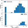 |
Fig. 5. Distributions of offsets of the CG4 positions relative to their host PC group, computed between group centroids (top) and between brightest group galaxies (bottom) in virial units. The vertical lines indicate the medians (0.23 for the centroids and 0 for the BGGs). In both panels the null values were clipped to 0.001. The peaks at 0.001 in the upper panel correspond to perfect matches between the CG4 and RG4 groups, while those in the bottom panel correspond to the CG4 and PC groups sharing the same BGG. |
3.3. Comparison to Zheng and Shen
Zheng & Shen (2021) performed one-way membership matching of the CGs of their recent catalog (Zheng & Shen 2020) relative to the Yang et al. (2007) groups in order to analyze the location of the compact groups relative to their parent groups and to split their CGs into four classes. We applied their classification to the CG4s using their nomenclature.
For our selection, all CG4 galaxies belong to Lim-Tempel groups (we note that 18 CG4s contain galaxies belonging to Lim-Tempel groups with fewer than four galaxies). Among our 78 CG4 groups, we note the following characteristics:
-
Sixteen (21%) are “Split” between several Lim-Tempel groups, similar to the 21% of Split CGs found by Zheng & Shen (2021). Among these 16 groups, 14 are split in two parent groups (four CG4s in a 2+2 configuration and ten are in a 3+1 configuration), while two are split between three parent groups (in a 2+1+1 configuration). Among the 32 Lim-Tempel groups hosting Split CG4 fragments, one group hosts Split CG4 galaxies coming from two different CG4s and one hosts galaxies coming from three different Split CG4s19.
-
Six (8%) are “Isolated”, i.e. they form a whole Lim-Tempel group by themselves, while Zheng & Shen (2021) found 27% of Isolated CGs.
-
Nineteen (24%) are “Predominant”, i.e non-Isolated, non-Split, and accounting for half or more of their host group total r-band luminosity, while Zheng & Shen (2021) reported 26%.
-
Thirty-seven (47%) are “Embedded”, i.e non-Isolated, non-Split, and accounting for less than half their host group total r-band luminosity, which is much higher that the 23% found by Zheng & Shen (2021).
Barnard tests between one class and all the others indicate that the lower fraction of Isolated groups and higher fraction of Embedded groups among CG4s relative to Zheng & Shen (2021) groups are both highly significant (p<10−4 and p<10−5, respectively). Therefore, while Zheng & Shen (2021) find roughly a quarter of each of their groups belonging to each category, our sample shows, in comparison, an excess of Embedded groups and a lack of Isolated groups.
The higher median multiplicity of the CG4s (4) compared to the Zheng & Shen (2020) groups (3) explains these two differences. All group catalogs show a rapidly decreasing multiplicity function. This can be explained by the expected correlation between group multiplicity and mass on one hand and the declining halo mass function (predicted first by Press & Schechter 1974, and confirmed later by numerous studies based on cosmological simulations). Triplets are considerably more frequent than quartets (2.4 times in Lim-Tempel and 7.6 times in Zheng & Shen 2020). By extension, Isolated triplets should be much more frequent than Isolated quartets. In fact, higher-multiplicity groups must be rarer than lower-multiplicity ones. Assuming Poisson statistics for the group multiplicity, i.e. the number of groups of multiplicity N is  , the ratio of counts of groups of N members over counts of groups of N+1 members is (N+1)/〈N〉. Thus, the ratio of numbers of groups of N = 3 members to groups of four is expected to be 4/〈N〉, i.e. ≃3.1 times more groups of three members than of four members for catalogs with 〈N〉 = 1.3, such as Lim-Tempel (see Table 1). This predicted ratio of 3.1 is consistent with the Zheng & Shen (2020) (27%) over CG4 (8±2%) fractions of Isolated compact groups (where the uncertainty is from Poisson statistics).
The relative preference for Embedded CG4s compared to those of Zheng & Shen (2020) may be caused by the lack of dwarf galaxies in the typically higher redshift Zheng & Shen (2020) CGs compared to our CG4s, selected at the same flux limit.
4. Properties
We now compare the properties of the different group samples and subsamples. We begin with the global group properties, and continue with the brightest group galaxy (BGG) location within their group in position, velocity and luminosity space. We then discuss group properties according to their location within their host groups and study correlations in CG4s. In a forthcoming article, we will compare and analyze the galaxy populations in the different samples.
4.1. Group properties
The distributions of these group properties are shown in Table 2 and displayed for the six most important global parameters in Fig. 6. Table 2 lists the median quantities and the probabilities that the median quantities of the Control4B, Control4C, and RG4 samples are consistent with those of the CG4 sample, using random shuffling (where the difference in medians is compared to those obtained in a large number of random sets of same size randomly drawn from the union of the two observed sets)20.
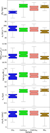 |
Fig. 6. Distributions of group properties for the different samples. From top to bottom, median of the projected inter-galaxy separations, radial velocity dispersion, group r-band luminosity, virial theorem mass, crossing time, and virial theorem mass to light ratio. The probabilities that the median quantities for the Control4B, Control4C, and RG4 samples are consistent with those of the CG4 sample are listed in Table 2. |
Comparison of median properties between compact group quartets and control samples of regular quartets.
Given that CG4s are selected to be high mean surface brightness, they should be small and/or luminous. Indeed, CG4s are much smaller than the groups in the control samples (first row of Table 2 and first panel of Fig. 6) and CG4s are also more luminous than RG4s (third row and panel). However, the Control4Bs are more luminous than the CG4s (third row and panel) because their galaxies are selected to be the four most luminous. There is no difference between the luminosities of CG4s and those of the cores of PC groups, i.e. Control4Cs.
The CG4 sample has the largest median radial velocity dispersion of the four samples (second row and panel). Given that the CG4 velocity dispersion notches in Fig. 6 do not overlap with the corresponding notches of the control samples, the median of CG4s is significantly different than the medians of the control samples (p<0.007 according to Table 2). This larger velocity dispersion of CG4s appears to be caused by a too permissive criterion to reject discordant redshifts. Indeed, the criterion of |v−median(v)|<1000 km s−1 initially introduced by Hickson et al. (1992) is equivalent to a >5 σ rejection criterion, which is much too liberal for redshift space selections. Most authors adopt 3 σ rejection criterion, while Mamon et al. (2010) found that 2.7 σ rejection is optimal to recover the velocity dispersions of clusters in cosmological simulations.
Table 2 also provides two measures of group mass: the proxy for the cosmological “virial” mass, ℳ200c (fourth row) and the virial theorem masses (Eq. [3], fifth row). The values of ℳ200c correspond to the total group mass, which are estimated by abundance matching between a known halo mass function and the observed group luminosity function (Lim et al. 2017). On the other hand, the virial theorem masses are measured within the sphere containing the galaxies, using  (Eq. [3]), which neglects a surface term that leads to an underestimation of the mass in clusters where only an inner subset of galaxies is considered (The & White 1986). Indeed, in the deeply embedded CG4s (Sect. 3 and Fig. 5), the virial theorem masses are much lower (by 0.31 dex, i.e. a factor of two) than the “virial” masses, while for the Control4B the difference in the logarithms of these two mass estimates is only 0.11 dex. Surprisingly, the Control4C sample of the four closest galaxies, which should also often be Embedded, shows only a 0.19 dex difference in the log mass estimates, perhaps because they are not so embedded since their median sizes are only one-third smaller than for the Control4Bs. It is also interesting to note that the RG4 sample shows a high difference of 0.25 dex between these two log mass estimates. While RG4s are extended, their low velocity dispersion leads to low virial theorem mass estimates, while their cosmological virial mass is less affected by their only moderately lower median luminosity.
When comparing the masses of the different group samples, one sees that both the cosmological virial masses and the virial-theorem masses of CG4s, Control4Bs, and Control4Cs are all higher than those of RG4s, because the former are usually embedded in larger groups (see Sect. 3 for the CG4s), while the latter, as mentioned above, have unusually low velocity dispersions. It is interesting to compare the virial theorem mass to luminosity ratios instead of the masses themselves. Only the Control4B subsample displays a significantly different (higher) median ℳVT/Lr compared to that for the CG4s, because the Control4Bs dominate the CG4s more in ℳVT (+0.15 dex) than in luminosity (+0.08 dex).
The crossing times of gravitating systems scale as one over square root of the mean density. It is therefore not surprising that CG4s, selected to be high surface brightness systems, and which turn out to be mostly small rather than luminous, have 2.5 to nearly 5 times shorter crossing times (Eq. [4]) than do the control groups (row 6).
4.2. Brightest group galaxies
We now analyze three properties of the BGGs relative to their group: 1) Their offset in position, 2) their offset in velocity, and 3) their fraction of the group luminosity and offset in absolute magnitude relative to the second most luminous galaxy.
4.2.1. Spatial offset
We define the relative offset in terms of the median inter-galaxy projected separation, 〈Rij〉. Therefore, the relative group spatial offset is  , where ΔBGG−cen is the projected physical separation between the BGG and the group centroid projected on the plane of sky. The distributions of these relative offsets are shown in the top panel of Fig. 7 and summarized in Table 2.
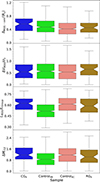 |
Fig. 7. Same as Fig. 6 but for properties related to the BGG. From top to bottom, relative BGGs offset from the group geometric center normalized to the median of the inter-galaxy separations, radial velocity of the BGG relative to the group in units of group velocity dispersion, BGG luminosity fraction, and magnitude gap between the BGG and the second brightest galaxy of the group. |
The BGGs in CG4s are significantly less centered than the BGGs in the control groups. As seen in the eighth row of Table 2, the median relative offsets are 0.56±0.03 for the CG4 sample, compared to 0.47±0.01 for Control4B, 0.42±0.01 for Control4C, and 0.45±0.03 for RG4, where the listed uncertainties are  ), with pi the ith percentile and N the sample size. This could be explained if CG4s are plagued by chance projections. However, one would then expect that CG4s show greater BGG relative velocity offsets compared to in the control samples, but this is not seen (see Sect. 4.2.2 below).
A simpler explanation is that Lim groups are built around BGGs, so relative to the group centroid, their BGG offsets are low, by construction, while they have no such bias for the BGG velocities. To be sure, we extracted a subsample of the Tempel et al. (2017) group catalog, which is based on a Friends-of-Friends algorithm, very different from the halo algorithm used to build the Lim et al. (2017) groups. Our subsample has the same restrictions as used for the CG4 and Lim groups: same bounds in redshift, absolute r-band magnitudes for the brightest and faintest members, as well as restricted to exactly four members. Those Tempel quartets have a median BGG offset of 0.50±0.03, and the significance of the difference with those of the control groups (estimated through 100 000 shuffles) are 14% with Control4B (median of 0.47), 7% with Control4C (median of 0.42) and 1.3×10⁻³ with RG4 (median of 0.45). Still, the median BGG offset of 0.56 of the CG4s is not significantly higher than that (0.50) of the similarly filtered Tempel quartets (p = 0.48).
4.2.2. Velocity offset
We computed the relative velocity offsets of the BGGs relative to their host groups as ΔvBGG/σv, which, applying Eq. (2) to the BGG, is equal to (zBGG−zgroup)/σz, where zgroup is the mean redshift of the members and σz=(1+zgroup) σv/c is the redshift dispersion, again according to Eq. (2). In contrast to their projected positions, the BGGs in CG4s do not show significantly different relative velocity offsets than those in regular group samples (see Table 2 and Fig. 7).
4.2.3. Dominance of the brightest group galaxy
We analyze the dominance of the BGG in two ways: 1) with the fraction of the total group luminosity contained in the BGG; 2) with the magnitude gap, ΔMr,12=Mr,2−Mr,1, i.e. the difference in the r-band rest-frame absolute magnitudes between the BGG and the second brightest galaxy of the group.
The third panel of Fig. 7 shows the fraction of the group luminosity contained in the BGG. The BGGs in CG4s are as dominant as those in the Control4C and RG4 group samples (the notches overlap). Control4B is the sample showing the least dominant BGGs and Table 2 indicates the BGG luminosity fraction in Control4Bs is significantly lower than in CG4s. This is expected by construction, since we picked the four brightest galaxies in a group, probably competing in luminosity with the BGG.
Similarly, the magnitude gaps of CG4s are as wide as those in the Control4C and RG4 group samples, while the Control4B sample shows significantly lower magnitude gaps. The median magnitude gaps are 1.17±0.09 for CG4, 0.85±0.03 for Control4B, 1.17±0.03 for Control4C, and 1.04±0.11 for RG4 (uncertainties on the medians:  , where σ means standard deviation).
Tremaine & Richstone (1977) proposed two statistics,
 (5)
(5)
to test the importance of magnitude gaps. They proved that T1 and T2 should both be greater than unity for cumulative luminosity functions that are single or double power-laws. Galaxy mergers tend to grow the most massive galaxy at the expense of the second-rank galaxy (Mamon 1987 for N-body simulations of virialized groups and Farhang et al. 2017 for groups in a cosmological context using SAMs), causing T1 and T2 to rapidly fall below unity (Mamon 1987).
We computed T1 and T2 for our four samples. Table 3 shows very low values of T2 and especially T1 for all four group samples. While values below unity were previously found for clusters (Tremaine & Richstone 1977) and the 2MASS compact groups (Díaz-Giménez et al. 2012), they were never found before for non-compact poor groups. This suggests that all four group samples have overluminous BGGs, most probably caused by mergers.
Tremaine-Richstone statistics for different group samples with identical selection criteria.
Tremaine-Richstone statistics samples built from other catalogs of compact and regular groups are displayed in the lower half of Table 3. These statistics are computed for subsamples filtered with the following criteria: 1) exactly four members; 2) the same maximum BGG redshift; 3) the same minimum BGG luminosity; 4) range in absolute magnitudes Mr,4−Mr,1≤3.
Table 3 indicates that all group samples besides D12 (the 2MCG sample from Díaz-Giménez et al. 2012) have T1 much lower than unity (T1≤0.4). The T1 values for the original HCG sample was 1.16 Mamon (1986), but this was due to a bias of the HCG sample against systems very dominated by a single galaxy (despite the magnitude concordance criterion, see Díaz-Giménez & Mamon 2010). For their full 2MCG sample, D12 found T1 = 0.51±0.06, precisely what is given in Table 3 for the “D12” subsample of 2MCG. The lower T1 values here appear to be the consequence of using volume-limited samples (restriction in redshift and absolute magnitude of the BGG that we imposed on the samples).
We used Lim-Tempel groups to test if our limits on group multiplicity on one hand and on redshift and luminosity range on the other could be the cause of our lower T1 values. As seen in Table 4, the imposition of a volume- and luminosity-limited sample for the BGGs drastically reduces the values of T1 because of the drastic reduction of the spread of BGG magnitudes with a small rise in the mean magnitude gap. Indeed, as seen in Fig. 1, going from the apparent magnitude cut for both the centrals and the satellites (oblique lines and oblique edge of shaded region) to the luminosity cut for both (horizontal lines) discards the groups with BGG luminosities below the cut, without affecting much the magnitude gap.
Tremaine-Richstone statistics of samples of Lim-Tempel groups with different selections.
4.3. CG4 properties according to their location within their host Lim-Tempel groups
In Sect. 3.3, we divided the CG4s into four Zheng & Shen (2021) classes: Split, Isolated, Predominant, and Embedded. We now analyze the possible dependencies of the properties of CG4s on the environment they inhabit. The properties of the four sub-samples of CG4s are displayed in Table 5.
Comparison of median properties of CG4 sub-samples according to their location in Lim-Tempel groups
The Split CG4s have significantly higher median velocity dispersion (366 km s−1) than the full set of CG4s (188 km s−1). In fact, the non-Split CG4s have a median velocity dispersion of only 160 km s−1. However, the median velocity dispersion of the RG4s is much lower at σv = 97 km s−1 (p = 10−5). This confirms our long-held suspicion that the velocity concordance criterion that all member galaxies must lie within ±1000 km s−1 from the median is too permissive, since it is over five times the median velocity dispersion of the full set of CG4s (Table 2) and roughly seven times the median velocity dispersion of non-Split CG4s. Filtering our CG4 sample to those whose velocities all lie within 500 km s−1 from the median (instead of 1000 km s−1), we find only 7 Split compact groups among 64, i.e. only 11% (instead of 25%)21. Therefore, the Split CG4s may be contaminated by galaxies that are chance-aligned with at least another group). This is corroborated by the low fraction of common BGGs between Split groups and their two or more host groups (row 2 of Table 5). This higher velocity dispersion of Split CG4s compared to other CG4s, at equal size, translates to higher virial theorem mass and mass-to-light ratio, as well as lower crossing time (rows 6 to 8 of Table 5) for the Split CG4s.
The Isolated CG4s display a large number of statistically significant (bold in Table 2) differences with the full set of CG4s: they have lower velocity dispersions, virial theorem masses, and magnitude gaps, as well as higher crossing times. The lower velocity dispersions of the Isolated CG4s compared to the Predominant and Embedded ones are probably the consequence of the higher multiplicities of the parent groups of these latter two classes of CG4s. These host groups may have galaxies outside of the CG4s on the plane of sky that are physically near their BGG (in real space), implying more mass at this physical distance to the BGG and hence a higher velocity dispersion. In turn, the lower velocity dispersions of Isolated CGs produce lower virial theorem masses and higher crossing times by the definitions of these quantities. Finally, the Isolated CG4s have significantly lower magnitude gaps (and marginally significantly lower BGG luminosity fractions) than the ensemble of CG4s. This is expected, since the Embedded and Predominant CG4s usually share the BGG of their host group (second row of Table 5), which is usually richer, more massive and with more luminous BGGs (Table 2).
We also note that the Isolated CG4s have indistinguishable median properties compared to the RG4s. Only CG properties that depend on group size, namely size, virial theorem mass, crossing time, and virial theorem mass-to-light ratio have significantly lower values than in the RG4s.
The Embedded CG4s have higher luminosity than the typical CG4, as expected by their definition of contributing over half the luminosity of the host group. Finally, the Predominant CG4s show no significant differences with the full sample, perhaps because they account for half the CG4 sample.
Row 8 does not display ℳ200c for the parent group of Split groups, because there is more than one parent. Predominant parent groups have the typical CG4 ℳ200c, while Isolated and Embedded ones are respectively more and less massive. Indeed, with exactly four members, CG4s lie in a narrow mass span compared to their parent groups. Therefore, Isolated parent groups are the CG4 itself and therefore less massive, while Embedded parent groups have to be large enough so that the considered CG4 is not Predominant.
4.4. Correlations of group properties
4.4.1. Luminosity segregation
In relaxed galaxy systems, (partial) energy equipartition should lead to mass segregation, where the most massive galaxies lie in the group center, while the low-mass ones will be able to probe the outskirts of the group. If luminosity traces mass, one would thus expect luminosity segregation with an anticorrelation between galaxy luminosity and distance to the group center. Luminosity segregation was predicted for CGs by Mamon (1987) and first detected in CGs by Díaz-Giménez et al. (2012), who saw no signs of it in other regular group samples22, nor in the original CG sample by Hickson et al. (1992), which is incomplete in systems with a dominant BGG (Díaz-Giménez & Mamon 2010).
Figure 8 displays the trend of galaxy luminosity fraction versus relative position in the group. There exists a luminosity segregation for CG4 that is also present in the control samples. The Spearman rank test of luminosity fraction of galaxies versus distance to centroid in median inter-distance units produces a significant anticorrelation (rS=−0.18, with a probability p = 0.01 of occurring by chance). The control samples show even stronger luminosity - radial distance anticorrelations.
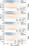 |
Fig. 8. Luminosity segregation in the four group samples: galaxy luminosity fraction versus relative position of galaxy relative to the group centroid. The panels show the kernel density estimator contour level lines for CG4, Control4B, Control4C, and RG4 from top to bottom, respectively. The BGGs are shown in blue and the satellites in orange. The rank correlations and corresponding p values (in percent) are displayed for all galaxies of the group (i.e., including BGGs) and for the satellite galaxies (i.e., non-BGGs) only. |
Given that BGGs are understood to grow by mergers (Mamon 1987), we also searched for luminosity segregation restricted to the satellites. Figure 8 shows that luminosity segregation among satellites is still detected in CG4s as well as in the control samples, but with far weaker (except in CG4s), yet still significant, correlations (except for RG4s).
We now consider luminosity segregation for the different CG4 Zheng & Shen (2021) classes. Isolated satellites show a significant luminosity segregation: rS=−0.48 (p = 0.04), despite containing only six groups. Surprisingly, the luminosity segregation is decreased and loses its statistical significance when adding the BGGs (rS=−0.20, p = 0.36). Interestingly, the Split CG4s are also the sites of significant luminosity segregation: rS=−0.24 (p = 0.05) for all member galaxies and rS=−0.27 (p = 0.007) when restricted to satellites. The other two CG4 subsamples do not show any significant luminosity segregation, whether for all galaxies or for just the satellites, except for a marginally significant segregation (rS=−0.15, p = 0.07) when all galaxies from Embedded groups are considered.
4.4.2. Other significant correlations within samples
Next, we searched for parameter correlations other than luminosity segregation. We excluded correlations that are caused by selection effects on CG4s:
-
Magnitude gap versus BGG luminosity fraction. They both measure the dominance of the BGG, relative to the second-ranked galaxy and to the group itself, respectively.
-
Group luminosity versus group size since compact groups are defined through a minimal surface brightness.
-
Group luminosity versus BGG luminosity fraction, because the product of the group luminosity and BGG luminosity fraction is the BGG luminosity, for which we set a lower limit (see Sect. 2).
-
Group luminosity versus magnitude gap since this parameter is correlated to the BGG luminosity fraction (see previous point).
Table 6 displays the significant correlations seen in the different group samples between group size, velocity dispersion, luminosity, BGG positional and velocity offsets, as well as luminosity fraction and magnitude gap, after discarding the correlations noted in the previous paragraph. The corresponding plots for all pairs of quantities showing significant correlations for at least one sample are displayed in Fig. 9.
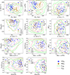 |
Fig. 9. Most significant correlations between quantities within samples as shown in Table 6. Quantities strongly correlated because of selection effects are not displayed – see main text. The legends provide the Spearman rank correlations, which are in bold if significant. |
Significant correlations between group properties.
The CG4 groups show only one significant correlation: group size (from the median projected separation) versus BGG relative offset (rS=−0.26, p = 0.024).
The other group samples show some significant correlations not seen in CG4s. The most significant of these are the anticorrelations of relative BGG offset with the dominance of the BGG (luminosity fraction of BGG or magnitude gap). This is an improvement over Skibba et al. (2011) who showed that the BGG does not lie at the geometric center of groups, and complementary to Gozaliasl et al. (2019) who showed that the BGG offset decreases with increasing halo mass, decreasing redshift and increasing magnitude gap. Also, the velocity dispersions of both Control4Bs and Control4Cs are correlated with their total luminosities. These velocity dispersions are even more correlated with the group masses, as expected from the virial theorem mass definition incorporating the group velocity dispersion, and from the Yang-Lim group finder algorithm that uses mass to predict velocity dispersion and deduce membership. Interestingly, the velocity dispersions of Control4Cs are correlated with their BGG luminosity fraction, while the opposite trend is significant for the Control4Bs. We found no significant correlations of properties for the RG4 sample, because of its much smaller size (as that of the CG4 sample) compared to those of the Control4Bs and Control4Cs.
5. Conclusions and final discussion
5.1. Conclusions
We have here compared a doubly-complete sample of compact groups, restricted to groups of four members to avoid multiplicity effects, to three carefully crafted control samples of regular groups. One consists of the groups of at least four members, from which we select the brightest group galaxy and its three closest satellites. Another consists of the groups of at least four members, from which we select instead the brightest group galaxy and its three brightest satellites. And the last one consists of regular groups of exactly four galaxies. This comparison led to the following conclusions.
-
A large majority of the CG4s are located in the cores of their host groups, and a vast majority of those share their BGG with their host group (Fig. 5).
-
Only a small fraction (8%) of the CG4s are identical to a Lim group. Furthermore, 10% of isolated regular Lim groups of four members are CG4s (Sect. 3.3).
-
The CG4s are smaller, as expected from their selection (Table 2 and Fig. 6).
-
The CG4s have higher velocity dispersions than ordinary groups (Table 2 and Fig. 6). This suggests that the velocity concordance criterion of <1000 km s−1 from the median for CG4s is too liberal, as it amounts to over 5 σv for the full set of CG4s and nearly 7 σv for those that are not split between two or more parent groups. Had we taken a 2.7 σ rejection criterion (Mamon et al. 2010), the maximum allowed difference with the median velocity would have been 500 km s−1 when including the Split CG4s and 400 km s−1 when discarding them (but see item #10 below). Furthermore, Zandivarez et al. (2024) found that CGs selected with a velocity concordance of 500 km s−1 have a 20% lower median velocity dispersion than when using the usual 1000 km s−1 velocity concordance limit. Reducing the velocity dispersion of CG4s by 20% would make the median velocity dispersion match that of Control4C.
-
The CG4s are less luminous than the Control4Bs (which is not surprising) and marginally less luminous than the Control4Cs but more luminous than the RG4s (Table 2 and Fig. 6).
-
The BGGs in CG4s have stronger relative spatial offsets than those in ordinary Lim-Tempel groups (Table 2 and Fig. 7). But those control groups are built according to the Yang et al. (2007) group finder updated by Lim et al. (2017), which builds the group around the BGG. Comparing instead to a similarly filtered sample of Tempel et al. (2017) groups of four galaxies shows no significant difference in BGG offsets (end of Sect. 4.2.1).
-
The BGGs in CG4s contribute to similar fractions of the group luminosity as do the control samples, except for the Control4Bs (Table 2 and Fig. 7), which are designed to host the four most luminous galaxies and are more likely to have similar absolute magnitudes instead of having a dominant one. Similarly, CG4s have similar magnitude gaps between the first- and second-ranked luminosity galaxies, as do the control groups, except for Control4Bs, which exhibit a smaller magnitude gap for the same reasons as above.
-
The CG4s show significant luminosity segregation, as do the three control group samples (Fig. 8). And even after removing the BGG, the remaining galaxies (i.e., satellites) show a significant luminosity segregation, and it is stronger than in the three control samples.
-
Only 8% of the CG4s, selected to be Isolated in redshift space are not associated with larger groups (Sect. 3.3), in contrast to 27% for the Zheng & Shen (2020) CGs of at least three galaxies (Zheng & Shen 2021), as expected from the decreasing multiplicity function of cosmic systems. Those Isolated CG4s are smaller (as expected from selection effects) and less massive than a typical non-compact group of four galaxies (i.e., an RG4).
-
One quarter of the CG4s are split between several regular groups (Sect. 3.3), which is the same fraction Zheng & Shen (2021) found for their CGs. The Split CG4s have much larger velocity dispersions (Table 5), suggesting that this subsample may be contaminated by spurious CGs caused by chance alignments of galaxies within unconnected groups. The Split CG4s also show significant luminosity segregation for all galaxies, even when discarding the BGGs and thus restricting Split CG4s to the satellites. But this luminosity segregation may be spurious (Sect. 4.4.1). For example, it may be caused by the superposition of regular groups of different characteristics along the line of sight.
In summary, apart from the properties directly affected by selection effects (high mean surface brightness, implying smaller and more luminous groups), the properties of compact groups of four galaxies selected to be truly isolated in redshift space (i.e., of the Isolated class) are quite similar to those of regular groups of galaxies. Hence, compact groups are not special. Our conclusion (based on observations) is both similar and complementary to that of Zandivarez et al. (2014), who compared the galaxy locations in mock CGs to mock regular groups in a SAM after supplementing the CGs with galaxies less luminous than the three-magnitude range limit. They found very similar galaxy surface density profiles in terms of the projected distance of “satellites” to the first- or second-ranked galaxy, normalized to the projected distance between these two brightest galaxies.
5.2. Particularities of CG4s and clues to their nature
Our results provide clues on the nature of compact groups of galaxies. Since the great majority of the CG4 BGGs are common to those of parent group BGGs, it is tempting to consider such compact groups as physically dense cores of parent groups. More precisely, CG4s would constitute the cores of regular groups that are fortunate to appear isolated along the line of sight.
However, having associations inside a parent group does not guarantee that these groups are physically dense. Indeed, it is common to have chance alignments along the line of sight of galaxies – or better pairs of galaxies – within groups, as predicted by Walke & Mamon (1989). This has been confirmed in semianalytical models of galaxy formation (Díaz-Giménez & Mamon 2010; Díaz-Giménez et al. 2020) and found by Mamon (2008) in a compact group previously discovered (Mamon 1989) inside the Virgo cluster using accurate redshift-independent distances23. An analysis of five different SAMs indicated that CGs, although selected to be isolated in redshift space, are very rarely isolated in 3D (Taverna et al. 2022). Combining this with their association with the cores of parent groups indicates that many CGs are indeed chance alignments of galaxies within larger groups, usually sharing the BGG. The CG4s that are split between several parent Lim groups are likely to be the most affected by such chance alignments, given their much higher velocity dispersions.
In a forthcoming study, we will analyze the links between compact group properties and their galaxy population. We will also compare the properties of galaxies in compact groups with those within the cores of regular groups.
Acknowledgments
We thank the anonymous referee for constructive comments after a very thorough reading of the manuscript. MT warmly thanks the Institut d’Astrophysique de Paris for its hospitality.
The capitalized words are defined in section 3.3.
Three HMCGs are split between four Lim groups: HMCG 359 (N = 6 members) has three galaxies in N = 4 Lim group 10218 and three galaxies in three separate Lim groups of a single galaxy; HMCG 415 (N = 5) has two galaxies in a Lim group of two galaxies and three galaxies in three separate Lim groups of a single galaxy; as another example, the four galaxies of HMCG 445 are split into four Lim groups with N = 11,8,3, and 1, respectively.
Available in the “SDSS DR7” section at https://gax.sjtu.edu.cn/data/Group.html
We do not use the grouping of Tempel et al. (2017), because it is based on Friends-of-Friends, and appears considerably less reliable than the Yang et al. (2007) algorithm (as shown by Duarte & Mamon 2015).
In this section, the three-magnitude maximum allowed for the difference between BGGs and satellites in CG4 groups concerns absolute magnitudes, instead of apparent magnitudes as used in other sections. There are five CG4s with maximum absolute magnitudes gaps (3.02, 3.06, 3.07, 3.18 and 3.25).
We neglected peculiar velocities, as we can expect the BGG velocity to be close to the velocity of the group's center of mass.
In the boxplot diagrams, the top and bottom lines of the boxes represent the 25th and 75th percentiles of the distributions, while the wrists of the boxes represent the medians. Notches display the confidence interval (95% confidence level) symmetrically around the medians. When comparing distributions, if the notches of two boxes do not vertically overlap, there is a statistically significant difference between the medians (McGill et al. 1978; Krzywinski & Altman 2014). For skewed distributions or small-sized samples, it might happen that the CI is wider than the 25th or 75th percentile. Therefore, the plot will display an “inside out” shape. The lines extending from the boxes are called whiskers (not shown in Fig. 2 but in Fig. 6). The boundary of the whiskers is based on the 1.5 inter-quartile range (IQR) value. The whiskers extend from the bottom (resp. top) of the boxes to the lowest (resp. highest) data point that falls within 1.5 times the IQR. The whisker lengths might not be symmetrical since they must end at an observed data point.
We define centroid by converting the equatorial coordinates to a cartesian frame on the unit sphere, taking the means and converting back to the equatorial frame.
There are only 32 Lim-Tempel groups hosting Split CG4 fragments instead of the expected 14×2+2×3 = 34 since one LT group hosts fragments from three different CG4s.
Random shuffling has two important advantages over classical non-parametric tests: 1) Shuffling immediately provides probabilities, while the probabilities for classical non-parametric tests are only known for simple (e.g., normal) distributions. 2) Shuffling allows one to compare a particular measure of a distribution, here median, while most classical non-parametric tests measure the consistency between two (full) distributions; thus they are sensitive to measures (e.g., spread) that are not interesting when only testing for a particular measure (e.g., median).
Actually, among 78 CG4s, three have σv≥500 km s−1 (the maximum CG4 velocity dispersion is 686 km s−1), all of which are Split groups. In fact, the five highest velocity dispersion CG4s are all Split.
Díaz-Giménez et al. (2012) did not analyze the Yang et al. (2005) group sample, which resembles the Lim et al. (2017) sample.
Admittedly, regular groups extracted with the Yang et al. (2007) group finder are also not immune to chance alignments, although probably less so than CGs given the latter's permissive accordant velocity criterion.
References
- Beers, T. C., Flynn, K., & Gebhardt, K. 1990, AJ, 100, 32 [Google Scholar]
- Blanton, M. R., & Roweis, S. 2007, AJ, 133, 734 [NASA ADS] [CrossRef] [Google Scholar]
- Blanton, M. R., Hogg, D. W., Bahcall, N. A., et al. 2003, ApJ, 592, 819 [Google Scholar]
- Bryan, G. L., & Norman, M. L. 1998, ApJ, 495, 80 [NASA ADS] [CrossRef] [Google Scholar]
- Burbidge, E. M., & Burbidge, G. R. 1961, AJ, 66, 541 [Google Scholar]
- Chilingarian, I. V., & Zolotukhin, I. Y. 2012, MNRAS, 419, 1727 [Google Scholar]
- Cole, S., & Lacey, C. 1996, MNRAS, 281, 716 [NASA ADS] [CrossRef] [Google Scholar]
- Díaz-Giménez, E., & Mamon, G. A. 2010, MNRAS, 409, 1227 [CrossRef] [Google Scholar]
- Díaz-Giménez, E., & Zandivarez, A. 2015, A&A, 578, A61 [NASA ADS] [CrossRef] [EDP Sciences] [Google Scholar]
- Díaz-Giménez, E., Mamon, G. A., Pacheco, M., Mendes de Oliveira, C., & Alonso, M. V. 2012, MNRAS, 426, 296 [Google Scholar]
- Díaz-Giménez, E., Zandivarez, A., & Taverna, A. 2018, A&A, 618, A157 [NASA ADS] [CrossRef] [EDP Sciences] [Google Scholar]
- Díaz-Giménez, E., Taverna, A., Zandivarez, A., & Mamon, G. A. 2020, MNRAS, 492, 2588 [Google Scholar]
- Duarte, M., & Mamon, G. A. 2015, MNRAS, 453, 3848 [Google Scholar]
- Dutton, A. A., & Macciò, A. V. 2014, MNRAS, 441, 3359 [Google Scholar]
- Farhang, A., Khosroshahi, H. G., Mamon, G. A., Dariush, A. A., & Raouf, M. 2017, ApJ, 840, 58 [Google Scholar]
- Gozaliasl, G., Finoguenov, A., Tanaka, M., et al. 2019, MNRAS, 483, 3545 [Google Scholar]
- Heisler, J., Tremaine, S., & Bahcall, J. N. 1985, ApJ, 298, 8 [CrossRef] [Google Scholar]
- Hickson, P. 1982, ApJ, 255, 382 [NASA ADS] [CrossRef] [Google Scholar]
- Hickson, P., & Rood, H. J. 1988, ApJ, 331, L69 [Google Scholar]
- Hickson, P., Mendes de Oliveira, C., Huchra, J. P., & Palumbo, G. G. 1992, ApJ, 399, 353 [Google Scholar]
- Krzywinski, M., & Altman, N. 2014, Nature Methods, 11, 119 [CrossRef] [Google Scholar]
- Lim, S. H., Mo, H. J., Lu, Y., Wang, H., & Yang, X. 2017, MNRAS, 470, 2982 [NASA ADS] [CrossRef] [Google Scholar]
- Liske, J., Baldry, I. K., Driver, S. P., et al. 2015, MNRAS, 452, 2087 [Google Scholar]
- Luo, A. L., Zhao, Y. -H., Zhao, G., et al. 2015, RAA, 15, 1095 [NASA ADS] [Google Scholar]
- Mamon, G. A. 1986, ApJ, 307, 426 [Google Scholar]
- Mamon, G. A. 1987, ApJ, 321, 622 [NASA ADS] [CrossRef] [Google Scholar]
- Mamon, G. A. 1989, A&A, 219, 98 [Google Scholar]
- Mamon, G. A. 2008, A&A, 486, 113 [NASA ADS] [CrossRef] [EDP Sciences] [Google Scholar]
- Mamon, G. A., Biviano, A., & Murante, G. 2010, A&A, 520, A30 [NASA ADS] [CrossRef] [EDP Sciences] [Google Scholar]
- McConnachie, A. W., Ellison, S. L., & Patton, D. R. 2008, MNRAS, 387, 1281 [Google Scholar]
- McConnachie, A. W., Patton, D. R., Ellison, S. L., & Simard, L. 2009, MNRAS, 395, 255 [NASA ADS] [CrossRef] [Google Scholar]
- McGill, R., Tukey, J. W., & Larsen, W. A. 1978, Am. Stat., 32, 12 [Google Scholar]
- Navarro, J. F., Frenk, C. S., & White, S. D. M. 1996, ApJ, 462, 563 [Google Scholar]
- Planck Collaboration XIII. 2016, A&A, 594, A13 [NASA ADS] [CrossRef] [EDP Sciences] [Google Scholar]
- Prandoni, I., Iovino, A., & MacGillivray, H. T. 1994, AJ, 107, 1235 [NASA ADS] [CrossRef] [Google Scholar]
- Press, W. H., & Schechter, P. 1974, ApJ, 187, 425 [Google Scholar]
- Rose, J. A. 1977, ApJ, 211, 311 [NASA ADS] [CrossRef] [Google Scholar]
- Schlegel, D. J., Finkbeiner, D. P., & Davis, M. 1998, ApJ, 500, 525 [Google Scholar]
- Skibba, R. A., van den Bosch, F. C., Yang, X., et al. 2011, MNRAS, 410, 417 [NASA ADS] [CrossRef] [Google Scholar]
- Sohn, J., Hwang, H. S., Geller, M. J., et al. 2015, J. Korean Astron. Soc., 48, 381 [NASA ADS] [CrossRef] [Google Scholar]
- Sohn, J., Geller, M. J., Hwang, H. S., Zahid, H. J., & Lee, M. G. 2016, ApJS, 225, 23 [NASA ADS] [CrossRef] [Google Scholar]
- Taverna, A., Díaz-Giménez, E., Zandivarez, A., & Mamon, G. A. 2022, MNRAS, 511, 4741 [CrossRef] [Google Scholar]
- Taverna, A., Salerno, J. M., Daza-Perilla, I. V., et al. 2023, MNRAS, 520, 6367 [CrossRef] [Google Scholar]
- Tempel, E., Tamm, A., Gramann, M., et al. 2014, A&A, 566, A1 [NASA ADS] [CrossRef] [EDP Sciences] [Google Scholar]
- Tempel, E., Tuvikene, T., Kipper, R., & Libeskind, N. I. 2017, A&A, 602, A100 [NASA ADS] [CrossRef] [EDP Sciences] [Google Scholar]
- The, L. S., & White, S. D. M. 1986, AJ, 92, 1248 [NASA ADS] [CrossRef] [Google Scholar]
- Tinker, J. L. 2021, ApJ, 923, 154 [NASA ADS] [CrossRef] [Google Scholar]
- Tremaine, S. D., & Richstone, D. O. 1977, ApJ, 212, 311 [NASA ADS] [CrossRef] [Google Scholar]
- Trevisan, M., Mamon, G. A., & Khosroshahi, H. G. 2017, MNRAS, 464, 4593 [Google Scholar]
- Wainer, H., & Thissen, D. 1976, Psychometrika, 41, 9 [CrossRef] [Google Scholar]
- Walke, D. G., & Mamon, G. A. 1989, A&A, 225, 291 [NASA ADS] [Google Scholar]
- Yang, X., Mo, H. J., van den Bosch, F. C., & Jing, Y. P. 2005, MNRAS, 356, 1293 [Google Scholar]
- Yang, X., Mo, H. J., Van den Bosch, F. C., et al. 2007, ApJ, 671, 153 [NASA ADS] [CrossRef] [Google Scholar]
- Zandivarez, A., Díaz-Giménez, E., Mendes de Oliveira, C., & Gubolin, H. 2014, A&A, 572, A68 [NASA ADS] [CrossRef] [EDP Sciences] [Google Scholar]
- Zandivarez, A., Díaz-Giménez, E., & Taverna, A. 2022, MNRAS, 514, 1231 [NASA ADS] [CrossRef] [Google Scholar]
- Zandivarez, A., Díaz-Giménez, E., Taverna, A., Rodriguez, F., & Merchán, M. 2024, A&A, 691, A6 [NASA ADS] [CrossRef] [EDP Sciences] [Google Scholar]
- Zheng, Y. -L., & Shen, S. -Y. 2020, ApJS, 246, 12 [NASA ADS] [CrossRef] [Google Scholar]
- Zheng, Y. -L., & Shen, S. -Y. 2021, ApJ, 911, 105 [CrossRef] [Google Scholar]
Appendix A: Conversion of virial masses and of virial radii
This appendix provides a simpler, yet more complete formalism than that of appendix A of Trevisan et al. (2017) to convert virial masses and virial radii, from a prior to final overdensity.
Given that the critical density of the Universe at epoch z is
 (A.1)
(A.1)
where  is the mean density of the Universe at epoch z, while E2(z)≡[H(z)/H0]2=Ωm,0(1+z)3+1−Ωm,0 for a flat Universe, the mass within the sphere (of radius rΔ) whose mean density is Δ times the critical (not mean) density of the Universe is
 (A.2)
(A.2)
Comparing now the mass of the same system within overdensities Δ and Δ′, Eq. (A.2) trivially yields
 (A.3)
(A.3)
Writing the mass profile as  , where rs is a universal attribute (e.g., the scale radius) of the density profile, while
  , one trivially obtains (independently of Eq. [A.3])
 (A.4)
(A.4)
where rΔ/rs≡cΔ is the concentration for the prior overdensity. Then, eliminating ℳΔ′/ℳΔ from Eqs. (A.3) and (A.4) yields
 (A.5)
(A.5)
The final radius, rΔ′ is then obtained by numerically solving Eq. (A.5) for rΔ′/rΔ. Then, the final mass, ℳΔ′ is deduced from either Eq. (A.3) or Eq. (A.4).24
The ratios rΔ′/rΔ and ℳΔ′/ℳΔ, calculated with Eqs. (A.5) and (A.3), are well approximated by second-order polynomial fits:
![Mathematical equation: $$ \frac {r_{\Delta '}}{r_{\Delta }} = \mathrm {dex}\sum _{i = 0}^2 a_i \left [\log _{10}\left (\frac {r_\Delta }{r_\mathrm {s}}\right )\right ]^i , $$](/articles/aa/full_html/2025/07/aa51713-24/aa51713-24-eq26.gif) (A.6a)
(A.6a)
![Mathematical equation: $$ \frac {{\cal {{M}}}_{\Delta '}}{{\cal {{M}}}_{\Delta }} = \mathrm {dex}\sum _{i = 0}^2 b_i \left [\log _{10}\left (\frac {r_{\Delta }}{r_\mathrm {s}}\right )\right ]^i, $$](/articles/aa/full_html/2025/07/aa51713-24/aa51713-24-eq27.gif) (A.6b)
(A.6b)
where rs is the scale radius of the halo (hence, rΔ/rs is the concentration of the halo in the prior system), with rms errors less than 0.0004 dex and 0.0015 dex for radius and mass ratios, respectively. For future users, we provide the coefficients of the polynomials in Table A.1 for some popular pairs of overdensities, for the NFW model (Navarro et al. 1996), for which (Cole & Lacey 1996)
 (A.7)
(A.7)
Coefficients of fits to ratios of z = 0 halo radii and masses.
There are two complications to using the simple Eq. (A.5) for converting virial radii and masses: 1) The group masses are defined using group overdensities relative to the mean density ρU(z) of the Universe, while it is more common to use overdensities relative to the critical density ρc(z) of the Universe. 2) In this context, Eq. (A.5) is insufficient, because the concentration c=rΔ/rs in the second term of its right-hand side, defined using the overdensity relative to  , is usually not as well known as is the concentration defined using the overdensity relative to ρc. Eq. (A.5) can be generalized by expressing the concentration cΔ in the original overdensity in terms of the known expression for the concentration cΔ′ in the new overdensity:
![Mathematical equation: $$ c_\Delta = \frac {r_\Delta }{r_\mathrm {s}} = \frac {r_\Delta }{r_\Delta ^{\prime }}\,c_\Delta ^{\prime }\left ({\cal {{M}}}_\Delta \,\frac {{\cal {{M}}}_\Delta ^{\prime }}{{\cal {{M}}}_\Delta }\right ) = \frac {r_\Delta }{r_\Delta ^{\prime }}\,c_\Delta ^{\prime }\left [{\cal {{M}}}_\Delta \,\frac {\Delta '}{\Delta }\,\left (\frac {r_\Delta ^{\prime }}{r_\Delta }\right )^3\right ], $$](/articles/aa/full_html/2025/07/aa51713-24/aa51713-24-eq30.gif) (A.8)
(A.8)
where the second equality is obtained using Eq. (A.3). Inserting Eq. (A.8) into Eq. (A.5) yields
![Mathematical equation: $$ {\Delta '\over \Delta }\, \left ({r_{\Delta '}\over r_\Delta }\right )^3 = \widehat M \left [{r_{\Delta '}\over r_\Delta }, \frac {r_\Delta }{r_\Delta ^{\prime }}\,c_\Delta ^{\prime }\left ({\cal {{M}}}_\Delta \,\frac {\Delta '}{\Delta }\,\left (\frac {r_\Delta ^{\prime }}{r_\Delta }\right )^3\right )\right ], $$](/articles/aa/full_html/2025/07/aa51713-24/aa51713-24-eq31.gif) (A.9)
(A.9)
which can be numerically solved for  , knowing the ratio of overdensities, Δ′/Δ, and the mass for the initial overdensity, ℳΔ. The mass ratio is then deduced from Eq. (A.3) and can be checked using Eq. (A.4).
We now discuss how we converted the masses ℳ180m to ℳ200c in Sect. 3.2. Analogous to Eq. (A.2), the mass within the radius of mean density equal to Δm times the mean density of the Universe is
 (A.10)
Then, by comparing the second equalities of Eqs. (A.2) and (A.10), the ratio of overdensity relative to ρc(z) to overdensity relative to  is
is
 (A.11)
We note that combining Eqs. (A.3) and (A.11), leads to a mass ratio:
 (A.12)
Inserting Eq. (A.11) into Eq. (A.9), yields
![Mathematical equation: $$ \frac {\Delta '}{\Omega _{\mathrm {m},0}\,\Delta _\mathrm {m}} \,\frac {E^2(z)}{(1+z)^3}\, \left ( \frac {r_{\Delta '}}{r_{\Delta ,\mathrm {m}}} \right )^3 =\widehat M \left\{ {r_{\Delta '}\over r_\Delta }, {r_\Delta \over r_\Delta ^{\prime }}\, c\left [\frac {\Delta '/\Delta _\mathrm {m}}{\Omega _{\mathrm {m},0}} \,\frac {E^2(z)}{(1+z)^3}\, \left ( \frac {r_{\Delta '}}{r_{\Delta ,\mathrm {m}}} \right )^3 \,{\cal {{M}}}_{\Delta ,\mathrm {m}}\right ]\right\} , $$](/articles/aa/full_html/2025/07/aa51713-24/aa51713-24-eq37.gif) (A.13)
(A.13)
which can be numerically solved for rΔ′/rΔ,m. The mass ratio is then deduced using Eqs. (A.3) and (A.11) and can be verified using Eq. (A.4).
Hence, Δ = 180 Ωm≃55.44 and Δ′ = 200. We adopted the z = 0 concentration-mass relation of Dutton & Macciò (2014) for Δ′ = 200c, i.e.
 (A.14)
Inserting Δ = 55.44 and Δ′ = 200 in Eq. (A.13), we ended up solving
![Mathematical equation: $$ 3.61\left (\frac {r_\mathrm {200c}}{r_\mathrm {180m}}\right )^3 = \widehat M\left\{ \frac {r_\mathrm {200c}}{r_\mathrm {180m}}, \frac {1}{3.61}\,c_\mathrm {200c}\left [3.61\left (\frac {r_\mathrm {200c}}{r_\mathrm {180m}}\right )^3 {\cal {{M}}}_\mathrm {180m}\right ] \right\} $$](/articles/aa/full_html/2025/07/aa51713-24/aa51713-24-eq39.gif) (A.15)
(A.15)
for r200c/r180m (where 3.61 = 200/55.44). Numerically solving Eq. (A.15), we found the following power-law approximations:
 (A.16a)
 (A.16b)
for our choice of the z = 0 Dutton & Macciò (2014) concentration-mass relation (Eq. A.14), as well as Ωm = 0.308. The very shallow power-laws are a consequence of the shallow concentration-mass relation (Eq. [A.14]) and the logarithmic increase of NFW mass with radius in the envelope (r180m>r200c>3 rs). Eqs. (A.16a) and (A.16b) are both precise to 0.2% rms for 12<log(h ℳ180m/M⊙)<15. Slight changes in the cosmological parameters should only have a very small effect.
All Tables
Comparison of median properties between compact group quartets and control samples of regular quartets.
Tremaine-Richstone statistics for different group samples with identical selection criteria.
Tremaine-Richstone statistics of samples of Lim-Tempel groups with different selections.
Comparison of median properties of CG4 sub-samples according to their location in Lim-Tempel groups
All Figures
|
Fig. 1. Absolute r-band magnitude versus redshift for galaxies in the HMCG compact group sample and in the CG4 subsample. The colors are gray for all HMCG galaxies, red for CG4 BGGs and blue for CG4 satellites. The shaded gray region represents galaxies fainter than the SDSS flux limit (r>17.77). The dotted line denotes our doubly complete HMCG sample, while the thick dash-dotted lines shows the magnitude and redshift limits for the BGGs. The oblique line is three magnitudes above the SDSS flux limit and is our limit for BGGs in the first-step CG4 selection process. |
| In the text | |
|
Fig. 2. Comparison of CG4 properties with samples of compact quartets built from other published compact group catalogs, with the same selection in redshifts and magnitudes: 0.005≤zBGG≤0.0452, MBGG≤−21.81, and M4−M1≤3. From top left to bottom right, the properties are median of the projected inter-galaxy separations, radial velocity dispersion, total group luminosity, group virial theorem mass, crossing time, mass-to-light ratio, BGG relative offset (normalized distance of the BGG to the centroid of the group), BGG relative velocity offset (normalized distance in radial velocity of the BGG to the group radial velocity dispersion, top-right panel), BGG luminosity fraction, and absolute magnitude difference between the two brightest galaxy members. The abscissa indicate the compact group catalogs: HCG: Hickson et al. (1992), D12: Díaz-Giménez et al. (2012), S16: Sohn et al. (2016), Z20: Zheng & Shen (2020), Z22: Zandivarez et al. (2022), D18: Díaz-Giménez et al. (2018), and CG4: this work. |
| In the text | |
|
Fig. 3. Multiplicity functions of the parent group samples: LT, LTz,Mr (step 2 in Sect. 2.4), and PC (step 4 in Sect. 2.4) in the range 4≤Ngalaxies≤20 (Ngalaxies reaches 538 for PC). The 62 PC groups of four correspond to the RG4 sample. |
| In the text | |
|
Fig. 4. Absolute magnitude difference between the BGG and the second brightest galaxy of each group versus group multiplicity for PC groups. |
| In the text | |
|
Fig. 5. Distributions of offsets of the CG4 positions relative to their host PC group, computed between group centroids (top) and between brightest group galaxies (bottom) in virial units. The vertical lines indicate the medians (0.23 for the centroids and 0 for the BGGs). In both panels the null values were clipped to 0.001. The peaks at 0.001 in the upper panel correspond to perfect matches between the CG4 and RG4 groups, while those in the bottom panel correspond to the CG4 and PC groups sharing the same BGG. |
| In the text | |
|
Fig. 6. Distributions of group properties for the different samples. From top to bottom, median of the projected inter-galaxy separations, radial velocity dispersion, group r-band luminosity, virial theorem mass, crossing time, and virial theorem mass to light ratio. The probabilities that the median quantities for the Control4B, Control4C, and RG4 samples are consistent with those of the CG4 sample are listed in Table 2. |
| In the text | |
|
Fig. 7. Same as Fig. 6 but for properties related to the BGG. From top to bottom, relative BGGs offset from the group geometric center normalized to the median of the inter-galaxy separations, radial velocity of the BGG relative to the group in units of group velocity dispersion, BGG luminosity fraction, and magnitude gap between the BGG and the second brightest galaxy of the group. |
| In the text | |
|
Fig. 8. Luminosity segregation in the four group samples: galaxy luminosity fraction versus relative position of galaxy relative to the group centroid. The panels show the kernel density estimator contour level lines for CG4, Control4B, Control4C, and RG4 from top to bottom, respectively. The BGGs are shown in blue and the satellites in orange. The rank correlations and corresponding p values (in percent) are displayed for all galaxies of the group (i.e., including BGGs) and for the satellite galaxies (i.e., non-BGGs) only. |
| In the text | |
|
Fig. 9. Most significant correlations between quantities within samples as shown in Table 6. Quantities strongly correlated because of selection effects are not displayed – see main text. The legends provide the Spearman rank correlations, which are in bold if significant. |
| In the text | |
Current usage metrics show cumulative count of Article Views (full-text article views including HTML views, PDF and ePub downloads, according to the available data) and Abstracts Views on Vision4Press platform.
Data correspond to usage on the plateform after 2015. The current usage metrics is available 48-96 hours after online publication and is updated daily on week days.
Initial download of the metrics may take a while.