| Issue |
A&A
Volume 698, June 2025
|
|
|---|---|---|
| Article Number | A156 | |
| Number of page(s) | 10 | |
| Section | Galactic structure, stellar clusters and populations | |
| DOI | https://doi.org/10.1051/0004-6361/202554212 | |
| Published online | 12 June 2025 | |
Nearby open clusters with tidal features: Golden sample selection and 3D structure
1
School of Physics and Optoelectronic Engineering, Anhui University,
Hefei
230601,
China
2
Purple Mountain Observatory, Chinese Academy of Sciences,
Yuanhua Road 10,
Nanjing
210023,
China
3
Shanghai Astronomical Observatory, Chinese Academy of Sciences,
80 Nandan Road,
Shanghai
200030,
China
4
Instituto de Astrofísica, Dep. de Ciencias Físicas, Facultad de Ciencias Exactas, Universidad Andres Bello,
Av. Fernández Concha 700,
Santiago,
Chile
5
Purple Mountain Observatory and Key Laboratory of Radio Astronomy, Chinese Academy of Sciences,
Yuanhua Road 10,
Nanjing
210033,
China
6
School of Astronomy and Space Science, University of Science and Technology of China,
Hefei
230026,
China
★ Corresponding author: This email address is being protected from spambots. You need JavaScript enabled to view it.
Received:
21
February
2025
Accepted:
23
April
2025
Abstract
Open clusters offer unique opportunities to study stellar dynamics and evolution under the influence of their internal gravity, the Milky Way’s gravitational field, and the interactions with encounters. Using the Gaia DR3 data for a catalog of open clusters within 500 parsecs that exhibit tidal features reported by the literature, we applied a novel method based on 3D principal component analysis to select a “golden sample” of nearby open clusters with minimal line-of-sight distortions. This approach ensures a systematic comparison of 3D and 2D structural parameters for tidally perturbed clusters. The selected golden sample includes Blanco 1, Melotte 20, Melotte 22, NGC 2632, NGC 7092, NGC 1662, Roslund 6, and Melotte 111. We analyzed these clusters by fitting both 2D and 3D King Profiles to their stellar density distributions. Our results reveal systematic discrepancies, with most of the golden sample clusters exhibiting larger 3D tidal radii compared to their 2D counterparts, demonstrating that the 2D projection effects bias the measured cluster size. Furthermore, the 3D density profiles show stronger deviations from the King profiles at the tidal radii (Δρ3D > Δρ2D), highlighting enhanced sensitivity to tidal disturbances. Additionally, we investigated the spatial distribution of cluster members relative to their bulk motion in the Galactic plane. We find that some clusters exhibit tidal features oriented perpendicular to their direction of motion, which can be attributed to the fact that the current surveys only detect the curved inner regions of the tidal features. In conclusion, this work offers a golden sample of nearby open clusters that are most reliable for 3D structure analysis and underscores the necessity of 3D analysis when characterizing OC morphological asymmetries, determining cluster size, and identifying tidal features.
Key words: methods: data analysis / catalogs / parallaxes / proper motions / open clusters and associations: general / open clusters and associations: individual: NGC 752
© The Authors 2025
 Open Access article, published by EDP Sciences, under the terms of the Creative Commons Attribution License (https://creativecommons.org/licenses/by/4.0), which permits unrestricted use, distribution, and reproduction in any medium, provided the original work is properly cited.
This article is published in open access under the Subscribe to Open model. This email address is being protected from spambots. You need JavaScript enabled to view it. to support open access publication.
1 Introduction
Open clusters (OCs) are key laboratories for studying the Galactic structure (see, e.g., Dias & Lépine 2005; Castro-Ginard et al. 2021; Joshi & Malhotra 2023), stellar evolution (see, e.g., Bertelli Motta et al. 2018; Jian et al. 2024), star formation history (see, e.g., Magrini et al. 2017; Spina et al. 2022; Bragaglia et al. 2024), and the evolution of the Milky Way (see, e.g., Kroupa 2005; Magrini et al. 2017; Fu et al. 2022). As gravitationally bound groups of stars formed nearly simultaneously from the same molecular cloud (Lada & Lada 2003), OCs offer a unique opportunity to explore stellar dynamics and the influence of the Galactic environment. The dynamical evolution of OCs, driven by internal processes and gravitational interactions with the Milky Way, often leads to the formation of tidal features, such as tidal tails. These features reflect the cluster mass loss and dynamical evolution within the cluster (see, e.g., Spitzer 1958; Lamers et al. 2005). Over time, the cluster continues to lose mass until it eventually disrupts and disperses all of its member stars to the Galactic field. By studying these tidal features and the intrinsic properties of the star clusters, we can gain valuable insights into the internal cluster processes (e.g., gas expulsion and mass segregation) (Dinnbier & Kroupa 2020; Liu et al. 2025; Alfonso et al. 2024; Angelo et al. 2025), external factors (e.g., the Galactic potential) (Wang & Jerabkova 2021; Kroupa et al. 2022), and the initial conditions of the Galactic field from which these stars originated (Hao et al. 2023; Casado & Hendy 2024).
Identifying tidal features and members of the Galactic OCs has historically been a challenging task, particularly in the pre-Gaia era, when precise astrometric data, such as stellar proper motions and parallaxes, were unavailable for a great number of stars. Prior to the advent of Gaia, the identification of tidal features and cluster members primarily relied on less precise methods, including local density analysis and color-magnitude diagrams (CMDs; see, e.g., Dalessandro et al. 2015; Bica et al. 2019; Kharchenko et al. 2013; Bica et al. 2008; Dias et al. 2002; Kharchenko et al. 2005; Piskunov et al. 2007; Platais et al. 1998; Alessi et al. 2003; Drake 2005). These methods, while useful, were often limited in their ability to reliably distinguish true tidal features from field star contamination.
The advent of the Gaia mission (Gaia Collaboration 2016) revolutionized the study of OCs. With its high-precision astrometric and photometric data, released in successive Gaia data deliveries (Gaia Collaboration 2017, 2018, 2021, 2023), researchers have been able to identify numerous new OCs and their member stars (e.g., Cantat-Gaudin et al. 2018; Cantat-Gaudin 2022; Hao et al. 2022; He et al. 2023; Zhong et al. 2022; Noormohammadi et al. 2023; Perren et al. 2023; van Groeningen et al. 2023; Qin et al. 2023). The observational confirmation of long ago predicted OC tidal tails has also become possible with Gaia (Meingast & Alves 2019; Röser et al. 2019). Since Gaia became operational, extended tidal features, especially in nearby OCs, have also become a focal point of discussion (see, e.g., Bhattacharya et al. 2022; Kos 2024; Risbud et al. 2025). Among these features, tidal tails of nearby OCs have been traced out to a total extent of almost 1 kpc when combined with N-body simulations (Jerabkova et al. 2021). And the detailed structure of the tidal tails has profound implications for cluster age dating (Dinnbier et al. 2022) and testing gravitational theory (Kroupa et al. 2024).
The structure parameters of OCs exhibiting tidal structures are typically determined through two-dimensional analyses. These analyses are often conducted using equatorial coordinates, right ascension (RA), and declination (Dec; see, e.g., Hunt & Reffert 2023; Zhong et al. 2022; Camargo 2021; Gao 2019; Rui et al. 2019; Yeh et al. 2019; Hosek et al. 2015) or the Galactic longitude (l) and latitude (b) (see, e.g., Gao 2024). To mitigate the projection effects, particularly for nearby OCs or those at high declinations, projected 2D coordinates are also employed to characterize the structure of OCs (see, e.g., Olivares et al. 2018; Tarricq et al. 2022).
While 2D analyses provide valuable information, 3D studies may offer a more comprehensive picture of cluster morphology and dynamics and thus allow for direct comparisons with N-body simulations (see, e.g., Wang et al. 2016) to reveal the true spatial distribution of stars both within and around the out-skirts of clusters. However, the 3D structure of OCs with tidal features has been less explored in the literature. A major challenge in analyzing the 3D structure of OCs is the pronounced artificial elongation of the clusters along the line of sight, which can arise from the propagation of parallax uncertainties (see, e.g., the discussions in Bailer-Jones 2015; Li & Shao 2025). Parallax inversion, the simplest method for deriving distances, may introduce complications, even for cluster member stars with symmetric parallax distributions, and the resulting distance distributions would become asymmetric. This effect was analyzed in detail by Luri et al. (2018) using Gaia DR2 data and further investigated by Piecka & Paunzen (2022), who quantified the impact of parallax uncertainties on the 3D morphology of clusters. They concluded that for a fixed parallax uncertainty, the apparent elongation of a cluster becomes more severe with increasing distance. Based on these findings, they recommended excluding OCs beyond 500 pc when studying 3D structures, as these clusters are more susceptible to such distortions.
To reduce the line-of-sight distortions in the 3D structure of OCs caused by parallax uncertainties, several studies have developed and applied distance corrections for OC member stars. For instance, Carrera et al. (2019) and Pang et al. (2021) adopted the Bayesian approach suggested by Bailer-Jones (2015) to derive the 3D morphology of OCs, utilizing their preferred priors. Similarly, Meingast et al. (2021) refined the distances of their OC member stars by employing a mixture of 3D Gaussians as a distance prior combined with the Gaussian likelihood derived from Gaia parallax measurements.
Another approach to mitigate the effects of line-of-sight elongation is to carefully select a sample of OCs that are less affected by such distortions. In this work, we adopt a 3D principal component analysis (PCA) method to identify nearby OCs that exhibit minimal line-of-sight elongation effects. This approach enables us to construct a “safe” sample of OCs, which we use to investigate how tidal interactions shape cluster morphology, compare results from 2D and 3D modeling, and assess the influence of the Galactic potential on cluster structure and longevity.
The paper is organized as follows. In Sect. 2, we describe the data used in this work. In Sect. 3, we outline the selection of our golden sample clusters. We analyze the tidal radius and tidal structure in Sect. 4. The results are discussed in Sect. 5. Finally, we summarize our results and conclusions in Sect. 6.
2 Data
The catalog by Tarricq et al. (2022, hereafter T22) serves as the basis of our work. It is a catalog of OCs with tidal features based on Gaia EDR3 data. The authors focus on 389 OCs with heliocentric distances of less than 1.5 kpc and ages greater than 50 Myr selected from the well-known OC list of Cantat-Gaudin et al. (2020, hereafter CG20). The stars identified in T22 are within 50 pc of their cluster centers and meet the following criteria: G < 18 mag, re-normalized unit weight error (RUWE)<1.4, and proper motion within 10 σ of the cluster’s bulk value. For clusters within 500 pc, the authors of T22 applied an additional cut on the parallax to exclude stars with astrometric measurements inconsistent with the cluster’s mean astrometric parameters. Cluster membership in T22 was determined using the unsupervised machine learning algorithm HDBSCAN (Hierarchical Density-Based Spatial Clustering of Applications with Noise, McInnes et al. 2017). A key objective of the T22 catalog is to include stars at the edges of OCs in order to enable the identification of tidal structures, which was not available in the CG20 membership lists. Following the recommendations of T22’s authors, we selected stars with membership probabilities of 0.5 or higher as members of these OCs.
3 Golden sample selection
In this section, we describe our methodology for selecting a subset of T22 OCs that are minimally affected by line-of-sight distortions, rendering them suitable for 3D structural studies. We refer to these OCs as our “golden sample”. Specifically, we identified these clusters by examining the alignment of their 3D PCA principal axis with the line of sight after applying the parallax zero-point correction to the member stars.
3.1 Parallax zero-point correction
The Gaia parallax solution has been known to exhibit biases since DR2 (see, e.g., Chan & Bovy 2020) that depend on the source’s projected position (Lindegren et al. 2018) as well as its magnitude and color (Zinn et al. 2019). Lindegren et al. (2021) extensively discussed the systematic offset of the Gaia EDR3 parallax. To address this bias, they employed quasars, stars in the Large Magellanic Cloud, and binaries to derive the parallax zero-point offset. The corresponding parallax zero-point offset values are calculated using the Python package gaiadr3_zeropoint1 by inputting the following parameters: the G-band magnitude (phot_g_mean_mag), the effective wavenumber (nu_eff_used_in_astrometry), the astrometrically estimated effective wavenumber (pseudocolour), and a five- or six-parameter solution (astrometric_params_solved).
For all OCs in the T22 catalog, we corrected the parallaxes of their member stars. The median of these median zero-point offsets is −0.0333 mas, with the smallest offset being −0.0266 ± 0.0114 mas and the largest being −0.0467 ± 0.0102 mas. After correcting the zero-point offset, all T22 OCs exhibited larger parallaxes corresponding to smaller distances. The standard deviation of distance among the member stars in each OC decreased slightly, indicating a marginally more compact distribution, though the variation is minimal. For OCs within 500 pc, the maximum change in the standard deviation of the distance is −2.74 pc; for those between 500 pc and 1000 pc, it is −7.92 pc; and for those beyond 1000 pc, it is 79.08 pc. After inverting the corrected parallaxes in order to derive the distances, the largest median distance correction within 500 pc is for UPK 24 (−11.895±3.544 pc). For clusters between 500 pc and 1000 pc, the largest correction is for NGC 6416 (−46.564±12.294 pc), and for clusters beyond 1000 pc, the largest correction is for UBC 326 (−108.056±37.153 pc). These corrections are essential for refining distance estimates and reducing the line-of-sight elongation caused by the parallax zero-point offset.
3.2 3D PCA alignment with the line of sight
After correcting the parallaxes, we performed the 3D PCA on all the T22 OCs using their Galactocentric Cartesian coordinates (X, Y, Z). The goal was to identify OCs with minimal elongation effects along the line of sight. PCA (see Jolliffe & Cadima 2016, for a review) is a statistical method that determines the directions of the largest variance in a dataset with multi-dimensional variables. For our case with Galactocentric Cartesian coordinates (X, Y, Z), for each member star in an OC, the first principal axis of PCA captures the direction with the greatest “apparent” spatial variance.
These Galactocentric coordinates were calculated using the Python package astropy (Astropy Collaboration 2013), incorporating right ascension, declination, and the zero-point corrected parallax as described earlier. To account for uncertainties in these parameters, we applied Monte Carlo sampling with 10000 iterations to estimate the corresponding errors in (X, Y, Z). We adopted the solar position as [X, Y, Z]⊙ = [−8200.0, 0.0, 14.0] pc following McMillan (2017).
Most PCA implementations assume mean centering, making the results sensitive to outliers and scaling. However, for the OCs studied here, their Galactocentric Cartesian coordinates (X, Y, Z) are expected to exhibit asymmetry and skewed distributions due to tidal structures. In such cases, median centering provides a more representative central point around which the majority of the data congregates. Therefore, we centered the data by subtracting the median [X, Y, Z] values before performing the PCA.
The PCA process in this work involved three key steps. The first step was centering the data. We subtract the median 3D position from the Galactocentric coordinates [X, Y, Z] of all cluster member stars to centralize the dataset. Unlike typical PCA applications, where datasets consist of multi-dimensional heterogeneous variables that require standardization, Galactocentric coordinates are homogeneous spatial variables. Next we computed the first principal axis. We used the Python package sklearn (Pedregosa et al. 2011) to compute the first principal axis of the PCA. The PCA of the dataset was performed with the parameter “n_components” set to one, yielding the 3D vector (m, n, p) representing the dominant direction of variance. Finally, we re-centered the coordinate to express the first principal axis in Galactocentric Cartesian coordinates: ![Mathematical equation: $\[\frac{\left(X_{\mathrm{P} 1}-X_{0}\right)}{m}=\frac{\left(Y_{P 1}-Y_{0}\right)}{n}=\frac{\left(Z_{P 1}-Z_{0}\right)}{p}\]$](/articles/aa/full_html/2025/06/aa54212-25/aa54212-25-eq1.png) .
.
To assess whether an OC exhibits significant elongation along the line of sight, we used the angle between the line-of-sight vector to its center and the cluster’s first principal axis derived from the PCA. Specifically, the angle ϕ quantifies the alignment between the PCA axis and the line of sight to the cluster center. A small value of ϕ might indicate that the “dominant” spatial distribution of cluster members is strongly aligned with the line of sight, while a large ϕ may suggest a minimal elongation in the line-of-sight direction. We also note that this assumption is valid only if the tidal tail is not physically along the line of sight.
Figure 1 shows the distribution of the 3D angle ϕ as a function of heliocentric distance for all T22 OCs. In general, ϕ decreases with the heliocentric distance, likely suggesting a stronger impact from the line-of-sight distortion effect for distant OCs. Piecka & Paunzen (2022) recommended excluding clusters beyond 500 pc for cluster morphology studies, a threshold also adopted by Meingast et al. (2021) and Pang et al. (2021). Accordingly, we set an upper limit of 500 pc for our golden sample OCs. Indeed, Figure 1 clearly shows that ϕ values decrease significantly beyond ~500 pc (indicated by the vertical dashed line).
To ensure the statistical reliability of our structural analyses, we only retained clusters with at least 200 member stars (represented by gray filled circles in Figure 1). Additionally, any OCs lacking structure parameter determinations in T22 (marked with ×) were excluded for further analysis.
The combined selection based on distance and T22 structure parameters revealed a gap at ϕ ~ 30° in the ϕ-distance diagram. We used this gap to divide the remaining OCs into two categories: high ϕ and low ϕ. Figure 2 illustrates examples of both high ϕ and low ϕ clusters in the Galactocentric Cartesian coordinates (X, Y, Z), highlighting their PCA axis, the line of sight, and the 3D distribution of their member stars. We designated the clusters in the high ϕ category with ϕ > 30° as our golden sample because they exhibit minimal elongation along the line of sight. Since our goal is to define a conservative golden sample rather than a complete sample, there might be some clusters with genuine tidal structures that are excluded by our selection criteria. For example, cluster IC 4756 (ϕ = 15°) and NGC 752 (ϕ = 11.66°), both with ϕ < 30°, have been found to present tidal structures (Bhattacharya et al. 2021; Boffin et al. 2022; Ye et al. 2021). They are not selected in our golden sample but are listed as additional sample clusters because of their reported tidal tails. Moreover, as mentioned before, if an open cluster has the tidal tail physically along the line of sight, it will show a small ϕ. This might cause some correlation with the Galactic longitude. However, we excluded this possibility by statistically studying the listed Galactic coordinates and ϕ from the full Table 1.
In total, we have eight OCs in the golden sample containing a total of 4374 member stars. These clusters span a wide range of ages, from 51.3 Myr to 810 Myr, according to the T22 catalog. The central coordinates (X0, Y0, Z0) of the golden sample OCs along with their PCA first principal axis parameter (m, n, p), and the angle ϕ, are listed in Table 1. The corresponding parameters for all other T22 OCs are provided in the full version of the table, available at the CDS.
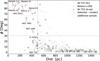 |
Fig. 1 Three-dimensional angle ϕ between the PCA axis and the line of sight to the cluster center as a function of distance for all 389 OCs in the T22 catalog. The OCs with more than 200 members are marked with gray filled circles, and those without structure parameters in the T22 catalog are marked with “×”. Red empty pentagrams are the selected golden sample OCs and are labeled with the cluster names. The red empty squares indicate IC 4756 and NGC 752, for reference. The horizontal gray dashed line represents the ϕ = 30° criteria, and the vertical gray dashed line indicates the 500 pc distance from the solar system barycenter. |
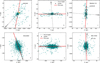 |
Fig. 2 Examples of cluster morphology in Galactocentric Cartesian coordinates. The upper panel shows Melotte 111 (a high-ϕ cluster), while the lower panel illustrates NGC 3532 (a low-ϕ example). The red lines denote the projection of the first principal PCA axis in 3D, and the gray dashed lines represent the solar position to the cluster center (marked by the black cross). |
4 Analysis with 3D data
Using the golden sample OCs – those exhibiting minimal elongation along the line of sight – we performed a 3D structural analysis. Specifically, we fit each cluster’s spatial distribution with a 3D King profile (King 1962) and examined its 3D morphology in relation to its Galactic motion. Before the analysis, we were already aware that the stellar membership of the T22 catalog may not be complete, so all results based on this catalog should be interpreted accordingly. One of the major factors contributing to the catalog’s incompleteness is that the cluster members are limited to 50 pc only, while in reality the tidal tails can extend to several hundred parsecs (see, e.g., Jerabkova et al. 2021; Kos 2024).
4.1 King profile fitting
To quantitatively characterize the structure of the selected golden sample OCs, we derived both 2D and 3D structure parameters by fitting a King profile (King 1962) to their respective number-density profiles. King profiles are widely used in the literature for fitting the density profile of open clusters. However, we call attention to the fact that the King profile is derived by assuming a spherically symmetrical mass distribution, and therefore, any structure deviating from this symmetry may bring errors to the fitting parameters. In this work, the King profile fitting suffices for our purpose of comparing the 2D and 3D structure parameters in the same manner despite its limits.
We employed a non-linear least squares approach to estimate the best-fit parameters. In this study, we adopted the following functional form:
![Mathematical equation: $\[n(R)=\left\{\begin{array}{ll}k\left(\frac{1}{\sqrt{1+\left(R / R_{\mathrm{c}}\right)^2}}-\frac{1}{\sqrt{1+\left(R_{\mathrm{t}} / R_{\mathrm{c}}\right)^2}}\right)^2+c, & \text { if } R<R_{\mathrm{t}} \\c, & \text { if } R \geq R_{\mathrm{t}}\end{array},\right.\]$](/articles/aa/full_html/2025/06/aa54212-25/aa54212-25-eq2.png)
where k is a proportionality constant related to the central density of the cluster, Rc is the core radius, Rt is the tidal radius, and n(R) represents either the 3D or 2D number density (in pc−3 or pc−2, respectively). The constant c accounts for the background level of field stars. Although our member stars are already of high probability, we followed Küpper et al. (2010a) to include a background term to improve the stability and quality of the King model fits.
To construct the 3D number-density King profile, we first computed the 3D radial distance of each star relative to the cluster center using
![Mathematical equation: $\[D_{\mathrm{C}}=\sqrt{\left(x-X_0\right)^2+\left(y-Y_0\right)^2+\left(z-Z_0\right)^2},\]$](/articles/aa/full_html/2025/06/aa54212-25/aa54212-25-eq3.png)
where X0, Y0, and Z0 are the median center coordinates listed in Table 1. We divided each cluster into 20 radial bins. The inner-most ten bins are spaced 1 pc apart, and the ten outer bins divide the radial range from 10 pc out to the furthest member star in equal logarithmic intervals. If the bin i contains no stars, it is merged with the adjacent bin i + 1. We took the mean radial distance of the stars in each bin to represent the bin’s distance to the cluster center. The corresponding 3D number density in a spherical shell with inner radius Di and outer radius Di+1 is defined as
![Mathematical equation: $\[\rho_{3 \mathrm{D}}=N / V=\frac{N}{4 / 3 \pi\left(D_{i+1}^3-D_i^3\right)},\]$](/articles/aa/full_html/2025/06/aa54212-25/aa54212-25-eq4.png)
where N is the number of stars in the bin. This procedure yields a set of paired values (D,ρ3D), which we used for the King profile fitting.
For the 2D case, we projected each star’s position onto a plane using the following equations (van de Ven et al. 2006; Olivares et al. 2018):
![Mathematical equation: $\[\begin{aligned}& x=D ~\sin \left(\alpha-\alpha_{\mathrm{c}}\right) ~\cos (\delta) \\& y=D\left[\cos \left(\delta_{\mathrm{c}}\right) ~\sin (\delta)-\sin \left(\delta_{\mathrm{c}}\right) ~\cos (\delta) ~\cos \left(\alpha-\alpha_{\mathrm{c}}\right)\right],\end{aligned}\]$](/articles/aa/full_html/2025/06/aa54212-25/aa54212-25-eq5.png)
where D is the heliocentric distance (in pc) of the cluster according to T22, and αc and δc are the median right ascension and declination of the cluster. The 2D radial distance for each star was computed as ![Mathematical equation: $\[R=\sqrt{x^{2}+y^{2}}\]$](/articles/aa/full_html/2025/06/aa54212-25/aa54212-25-eq6.png) . The binning strategy mirrors the 3D case. We formed 20 radial bins (merging any empty group with its neighbor) and took the average R within each bin. The 2D number density in a circular annulus surface is given by
. The binning strategy mirrors the 3D case. We formed 20 radial bins (merging any empty group with its neighbor) and took the average R within each bin. The 2D number density in a circular annulus surface is given by
![Mathematical equation: $\[\rho_{2 \mathrm{D}}=N / S=\frac{N}{\pi\left(R_{\mathrm{b}}^2-R_{\mathrm{a}}^2\right)},\]$](/articles/aa/full_html/2025/06/aa54212-25/aa54212-25-eq7.png)
where Ra and Rb are the inner and outer radii of the bin, respectively, and N is the number of stars in the bin. This process yielded a 2D radial number-density profile (R,ρ2D) for each cluster.
To fit the King profiles to both the 2D and 3D number-density profiles, we used the non-linear least squares method (via the Python package SciPy.optimize, Virtanen et al. 2020). In the fitting routine, we defined the residuals as (f(x) − y)/ey, where f(x) is the density obtained from the King function, y is the observed density, and ey is the Poisson uncertainty of y. From these fits, we obtained the core radius Rc, tidal radius Rt, background c, and proportionality constant k for each OC.
Basic properties of the input OC sample.
4.2 Cluster morphology to its motion
To explore the relationship between cluster morphology and the direction of motion, we used the Galactocentric Cartesian coordinates as calculated in Sect. 3.2 on the X-Y plane for further analysis. As an example of analysis, NGC 1662 is shown in Figure 3.
We determined the bulk motion of each cluster on this plane by computing the median velocity vector (see Table 2 for all golden sample clusters) of the member stars. The resulting vector, indicated by the gray arrow in Figure 3, defines the position angle θ = 0°, which we term the forward motion of the cluster. The opposite direction, θ = 180°, denotes the rearward direction relative to the cluster’s motion through the Milky Way.
This convention (θ = 0° and θ = 180°) is motivated by the well-known phenomenon of tidal structures in OCs. As an OC orbits the Galaxy, it can develop both leading and trailing tidal tails, where stars are preferentially stripped ahead of and behind the cluster along its orbit due to the differential gravitational forces in the Galaxy. By defining the cluster’s instantaneous motion vector in this way, we could examine whether the spatial distribution of the member stars exhibits elongations aligned with (or against) the direction of travel. In particular, an over-density of cluster members in the region near θ = 0° might be interpreted as a leading tidal feature, whereas an overdensity near θ = 180° could indicate a trailing tidal tail.
Figure 3 illustrates these morphology and motion considerations. The direction toward the Galactic center is shown by the horizontal black arrow, while the vertical black arrow indicates the direction of Galactic rotation. The black cross marks the adopted cluster center (see Table 1). The gray arrow, centered on the cluster, highlights the projected direction of future cluster motion (i.e., θ = 0°) in the X-Y plane. By combining the cluster morphology on the X-Y plane with these reference vectors, we could assess whether the distribution of the stars reveals an extended structure aligned with the orbit.
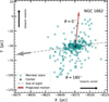 |
Fig. 3 NGC 1662 morphology in the Galactic X-Y plane. The member stars are represented as teal circles. The brown arrow indicates the future motion direction. For reference, the direction of the Galactic center and the galactic rotation are also illustrated. The line-of-sight direction to the cluster center (marked by the black cross) is also plotted (the gray dashed arrow). The position angles θ = 0° and θ = 180° represent the projected direction of the cluster’s forward motion and rearward direction. |
Bulk motion of the golden sample OCs and the two additional samples.
5 Results and discussions
Based on our selected OC golden sample, which exhibits minimal line-of-sight distortions and is suitable for 3D structure analysis (see Sect. 3 for the selection process), we present the results and the corresponding discussions in this section. Specifically, we examine the tidal radius differences between 3D and 2D analysis and the position angle density distribution relative to the direction of motion.
5.1 Tidal radius difference in 2D and 3D
The tidal radius of a star cluster determined with the King profile fitting represents the approximate distance from the cluster center beyond which stars are more likely to be stripped away by the gravitational field of the host galaxy than retained by the cluster’s self-gravity. A star cluster with a small tidal radius loses stars more rapidly due to tidal interactions with the Galaxy. From a dynamical perspective, we can roughly consider the tidal radius as the “edge” of the cluster, as stars beyond this radius are not bound to the cluster anymore.
A natural question is whether the tidal radius inferred from 2D projected data differs from the 3D intrinsic value. In other words, this refers to whether the choice of 2D or 3D analysis leads to different estimates of the cluster’s apparent edge. To address this question, we compared the King profile fitting results for our golden sample OCs in both 2D and 3D, as listed in Table A.1, with the fitting procedure described in Sect. 4.1.
Based on the same member star catalog, four of the golden sample OCs show a larger 3D tidal radius, Rt,3D, compared to their 2D tidal radius, Rt,2D. This indicates that these clusters appear to have a larger “edge” when analyzed in 3D than when using the conventional 2D method. However, four clusters – Melotte 111, Melotte 20, NGC 7092, and Roslund 6 – show nearly the same or a slightly smaller Rt,3D than Rt,2D. Figure 4 illustrates the 3D and 2D King profile fits for NGC 752, which has a pronounced discrepancy with Rt,3D = 71.02 pc (green vertical dotted line) versus Rt,2D = 29.23 pc (pink vertical dotted line), though it is in the additional sample. In the figure, the 3D data and the fitted King profile are represented by green triangles and a green dot-dashed line (with density on the left Y-axis), while the 2D data are marked with pink stars and a pink dashed line (with density on the right Y-axis). Although the King profile assumes a spherical symmetry, clusters with tidal structures can be elongated in different directions. Stars that are physically distant from the center along the line of sight may appear closer in projection, thereby biasing the density distribution inward and resulting in a smaller apparent 2D tidal radius. To test this speculation, we performed Monte Carlo simulations with 3D and 2D King profiles. We simulated star clusters and computed the corresponding 3D King profile number density ρ(r) and the projected 2D surface number density profile μ(r). By doing so, we were able to fit the 3D and 2D tidal radii with the same set of simulated data. We find that with the King profile in spherical symmetry, the 3D tidal radii are larger than the 2D ones, and the difference varies with the specific King profile parameters. However, we should not omit that the line-of-sight distortions (though minimized through our selection criteria), asymmetric tidal structures, and Poisson fluctuations may have also played important roles in the observed tidal radius difference in our sample.
To quantify how significantly the observed density profile deviates from the King model in 3D versus 2D analysis, we introduced the parameters Δρ3D and Δρ2D, which are defined as
![Mathematical equation: $\[\Delta \rho=\left(\rho_{\mathrm{obs}}-\rho_{\mathrm{mod}}\right) / \rho_{\mathrm{mod}},\]$](/articles/aa/full_html/2025/06/aa54212-25/aa54212-25-eq8.png)
where ρobs is the observed number density and ρmod corresponds to the King model number density. At the tidal radius, ρmod equals the background level of field stars c for a spherical symmetry cluster in equilibrium (see Sect. 4.1). A larger deviation of the observed number density from the King profile implies a more distorted cluster (see discussions in Dalessandro et al. 2015). Thus, Δρ3D and Δρ2D quantify the deviation of the observed number density from the model at the tidal radius, expressed in units of the background density c. In Figure 4, Δρ3D is shown as a dark green vertical shaded region, whereas Δρ2D (represented by a red shaded region) is so small that it is nearly invisible. The values for all OCs in our sample are summarized in Table A.1. For every cluster, Δρ3D is significantly larger than Δρ2D, suggesting that the 3D King profile provides a more sensitive indicator of tidal departures than the classical 2D approach.
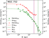 |
Fig. 4 Three- and two-dimensional King profile fitting for the cluster NGC 752. The X-axis represents the radial distance from the cluster center, the left Y-axis corresponds to the 3D density, and the right Y-axis corresponds to the 2D density. The pink stars, dashed line, and vertical dotted line indicate the observed 2D number density, the fitted King profile, and the corresponding tidal radius, respectively. Similarly, the green triangles, the dot-dashed line, and the vertical dotted line represent the 3D counterparts. For comparison, we overplot the tidal radius given by T22 as a blue solid vertical line. The deviation of the data from the 3D King profile at the tidal radius is highlighted with a dark green vertical shaded region. |
5.2 Density distribution in position angle
In Sect. 4.2, we analyzed the cluster morphology in the Galactic X-Y plane with respect to its bulk motion for each of the golden sample OCs with the aim of characterizing whether the member star distribution reveals any extended structure along the cluster’s motion in the Galactic plane. We quantified these potential tidal features by examining star count radial profiles as a function of θ and by comparing the derived density profiles in the leading (θ = 0°) versus trailing (θ = 180°) regions.
Figure 5 shows the fraction of cluster member stars as a function of position angle θ, measured counterclockwise around each cluster’s median velocity vector [U0, V0]. By design, θ = 0° (equivalently θ = 360°) corresponds to the leading direction of the cluster’s motion, whereas θ = 180° signifies the trailing direction. This figure illustrates whether the member stars are isotopically distributed in angle.
In the simplified picture of tidal stripping processes, one might expect that a strongly perturbed star cluster could show pronounced stellar overdensities in the forward (θ = 0°) and rearward (θ = 180°) directions (see, e.g., the simulated and observed star cluster tidal tails in Jerabkova et al. 2021; Kroupa et al. 2022). These directions respectively correspond to a “leading tail” and a “trailing tail” of stripped stars. However, from a straightforward inspection of Figure 5, none of the golden sample OCs shows a definitive peak at θ = 180° or θ = 0°. In fact, for several cases of our golden sample OCs, no overdensity as a function of the position angle θ is shown (e.g., Melotte 20 and Melotte 22), indicating that they do not present any clear tails around the cluster. For some other cases (e.g., NGC 1662, IC 4756, NGC 752, Roslund 6), density peaks appear near θ ≈ 90° or θ ≈ 270° rather than at the leading or trailing directions, suggesting that at least near the center of the cluster, tidal features may lie in a perpendicular orientation rather than parallel to the cluster’s instantaneous velocity vector.
This result does not contradict the picture that tidal tails align with the orbital path. In fact, it supports numerical simulations of OCs and their tidal tail structures. For instance, in the tidal tail simulations of Jerabkova et al. (2021), Kroupa et al. (2022), and Kroupa et al. (2024), the extended long tidal tails (approximately several hundred parsecs) more or less follow the motion of direction (θ = 0° or θ = 180° in our case); the angle of the tidal tail’s long axis evolves with the cluster age, as discussed extensively in Dinnbier et al. (2022); and the inner-most portion of the tidal tails often exhibits significant curvature, as discussed by Küpper et al. (2010b). If one focuses on a relatively small field around the cluster center (i.e., extending only out to a few tidal radii), the inner portion of each tail can appear to sweep “side-ways” in projection, creating a bend near the cluster center and appearing to have a near-perpendicular morphology before fanning out along the leading and trailing (~0°/180°) directions at larger distances.
Observationally, it is very rare that one can capture every stripped star out to large distances from the cluster, due to the limiting magnitude constraint in photometry and tidal density compared to field stars. If the data are truncated, one primarily sees the initial stages of the tidal arms, which may not yet be oriented parallel to a cluster’s motion vector. Indeed, the tidal structure OC catalog we adopted from T22 selected member stars that are only 50 pc from the cluster center, and the angular density histogram of Figure 5 is built only the relatively inner tidal part around the cluster center.
A sufficiently large survey area along the ~0°/180° direction of our sample OCs may result in more extended tidal tails, especially for the clusters showing two density peaks in the directions perpendicular to the cluster’s bulk motion. Figure 5 can serve as a finding chart for such studies in the future.
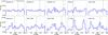 |
Fig. 5 Distribution of the member stars as a function of the position angle θ. The X-axis represents the position angle θ rotated counterclockwise around the projected motion [U0, V0] of the OCs. The solar position angle is indicated as the vertical gray dashed line. The 5% level is shown as a horizontal dot-dashed line to help the illustration. |
6 Summary
As a well-defined single stellar population, an OC serves as an ideal laboratory for studying the interplay between internal and external gravitational forces and the long-term evolution of star clusters. In this study, we have investigated the 3D structures of nearby OCs with tidal features based on the Tarricq et al. (2022) OC member catalog with tidal features. The catalog is based on high-precision astrometric data from the Gaia EDR3. While tidal structures in OCs have been extensively studied using 2D projections, analyzing their 3D morphology is essential to better understand their intrinsic structure and dynamical evolution. However, one of the major challenges in 3D studies of OCs arises from the systematic distortion effects introduced by parallax uncertainties, which can artificially elongate clusters along the line of sight. To address this issue, we have developed a new method based on three-dimensional PCA to identify a “golden sample” of OCs that are minimally affected by such distortions and thus allow for more reliable 3D structure analysis.
We limited our selection to clusters within 500 pc with more than 200 member stars. We then applied a parallax zero-point correction to refine the distance estimates for all member stars (see Sect. 3.1). Using PCA on the Galactocentric Cartesian coordinates of member stars, we measured the alignment between the 3D PCA first principal axis of each cluster and the observer’s line of sight (see Sect. 3.2). Clusters with a misalignment angle ϕ > 30° were selected to ensure a minimal elongation bias. The final golden sample consisted of eight OCs: Blanco 1, Melotte 20, Melotte 22, NGC 2632, NGC 7092, NGC 1662, Roslund 6, and Melotte 111. These OCs span ages from 51.3 Myr to 810 Myr, offering a diverse sample for probing dynamical evolution.
To characterize the structure of these clusters, we fit both 2D and 3D King profiles to their stellar density profiles. Our analysis revealed that, in most cases, the tidal radii derived from 3D modeling (Rt,3D) are systematically larger than those from 2D analysis (Rt,2D). This discrepancy may be because 2D projections tend to compress the apparent distribution of stars, leading to an underestimation of the tidal extent of the cluster.
We suggest using the King profile deviation at the tidal radius to characterize the cluster structure asymmetry. The 3D King model reveals greater deviations (Δρ3D) from observed densities at the tidal radius than 2D analyses (Δρ2D), indicating that 3D fitting better captures tidal distortions.
Beyond structural parameters, we explored the relationship between cluster morphology and motion in the Galactic plane. By analyzing the spatial distribution of cluster members relative to their bulk motion, we investigated whether OCs exhibit preferential elongation along or perpendicular to their direction of motion. Simplified tidal theory predicts that clusters should develop leading and trailing tidal tails aligned with their orbital trajectory due to differential gravitational forces from the Milky Way. More recent simulations and observations have revealed a more complex picture (Jerabkova et al. 2021; Kroupa et al. 2022; Dinnbier et al. 2022). Our analysis of the angular distribution of member stars supports this complex picture. While some clusters exhibit no preference for position angle, others display density peaks at perpendicular angles (~90° or ~270°). This feature can be interpreted as the inner part of the more extended leading or trailing tails at larger distances. Notably, the current member star catalog may only detect the initial phases of tidal tail development. Future extended surveys covering larger areas have a great potential to trace tails fully aligned with orbital motion.
This work highlights the importance of considering 3D morphology when interpreting the tidal structures of OCs. The traditional approach of using 2D projections can lead to biased conclusions regarding cluster size, shape, and dynamic state. The golden sample clusters identified in this work can serve as a benchmark for future studies of tidal interactions and their impact on cluster evolution.
Data availability
Full Table 1 is available at the CDS via anonymous ftp to cdsarc.cds.unistra.fr (130.79.128.5) or via https://cdsarc.cds.unistra.fr/viz-bin/cat/J/A+A/698/A156
Acknowledgements
We thank the anonymous referee for the kind and helpful comments, which helped to improve the paper’s clarity. We thank Dr. Yoann Tarricq and Dr. Xiaoying Pang for their useful discussions. We acknowledge National Natural Science Foundation of China (NSFC) No. 12003001, No. 12203100, No. 12303026, No. 12203099, the China Manned Space Project with No. CMS-CSST-2021-A08. C.Y. acknowledges the Natural Science Research Project of Anhui Educational Committee No. 2024AH050049 and the Anhui Project (Z010118169). L.L. thanks the support of the Young Data Scientist Project of the National Astronomical Data Center. M.F. acknowledges the National Key Research and Development Program of China (No. 2023YFA1608100). H.Z. is funded by China Postdoctoral Science Foundation (No. 2022M723373), and the Jiangsu Funding Program for Excellent Postdoctoral Talent. This work has made use of data from the European Space Agency (ESA) mission Gaia (http://www.cosmos.esa.int/gaia), processed by the Gaia Data Processing and Analysis Consortium (DPAC, http://www.cosmos.esa.int/web/gaia/dpac/consortium). This research has made use of the TOPCAT catalog handling and plotting tool (Taylor 2017); the Simbad database and the VizieR catalog access tool, CDS, Strasbourg, France; and NASA’s Astrophysics Data System.
Appendix A The structure parameters of OCs
Structure parameters of OCs.
References
- Alessi, B. S., Moitinho, A., & Dias, W. S. 2003, A&A, 410, 565 [NASA ADS] [CrossRef] [EDP Sciences] [Google Scholar]
- Alfonso, J., Vieira, K., & Garcia-Varela, A. 2024, A&A, submitted [arXiv:2410.23527] [Google Scholar]
- Angelo, M. S., Santos, Jr., J. F. C., Corradi, W. J. B., & Maia, F. F. S. 2025, MNRAS, 539, 2513 [Google Scholar]
- Astropy Collaboration (Robitaille, T. P., et al.) 2013, A&A, 558, A33 [NASA ADS] [CrossRef] [EDP Sciences] [Google Scholar]
- Bailer-Jones, C. A. L. 2015, PASP, 127, 994 [Google Scholar]
- Bertelli Motta, C., Pasquali, A., Richer, J., et al. 2018, MNRAS, 478, 425 [NASA ADS] [CrossRef] [Google Scholar]
- Bhattacharya, S., Agarwal, M., Rao, K. K., & Vaidya, K. 2021, MNRAS, 505, 1607 [NASA ADS] [CrossRef] [Google Scholar]
- Bhattacharya, S., Rao, K. K., Agarwal, M., Balan, S., & Vaidya, K. 2022, MNRAS, 517, 3525 [CrossRef] [Google Scholar]
- Bica, E., Bonatto, C., Dutra, C. M., & Santos, J. F. C. 2008, MNRAS, 389, 678 [Google Scholar]
- Bica, E., Pavani, D. B., Bonatto, C. J., & Lima, E. F. 2019, AJ, 157, 12 [Google Scholar]
- Boffin, H. M. J., Jerabkova, T., Beccari, G., & Wang, L. 2022, MNRAS, 514, 3579 [NASA ADS] [CrossRef] [Google Scholar]
- Bragaglia, A., D’Orazi, V., Magrini, L., et al. 2024, A&A, 687, A124 [NASA ADS] [CrossRef] [EDP Sciences] [Google Scholar]
- Camargo, D. 2021, ApJ, 923, 21 [NASA ADS] [CrossRef] [Google Scholar]
- Cantat-Gaudin, T. 2022, Universe, 8, 111 [NASA ADS] [CrossRef] [Google Scholar]
- Cantat-Gaudin, T., Jordi, C., Vallenari, A., et al. 2018, A&A, 618, A93 [NASA ADS] [CrossRef] [EDP Sciences] [Google Scholar]
- Cantat-Gaudin, T., Anders, F., Castro-Ginard, A., et al. 2020, A&A, 640, A1 [NASA ADS] [CrossRef] [EDP Sciences] [Google Scholar]
- Carrera, R., Pasquato, M., Vallenari, A., et al. 2019, A&A, 627, A119 [NASA ADS] [CrossRef] [EDP Sciences] [Google Scholar]
- Casado, J., & Hendy, Y. 2024, A&A, 687, A52 [NASA ADS] [CrossRef] [EDP Sciences] [Google Scholar]
- Castro-Ginard, A., McMillan, P. J., Luri, X., et al. 2021, A&A, 652, A162 [NASA ADS] [CrossRef] [EDP Sciences] [Google Scholar]
- Chan, V. C., & Bovy, J. 2020, MNRAS, 493, 4367 [Google Scholar]
- Dalessandro, E., Miocchi, P., Carraro, G., Jílková, L., & Moitinho, A. 2015, MNRAS, 449, 1811 [Google Scholar]
- Dias, W. S., & Lépine, J. R. D. 2005, ApJ, 629, 825 [NASA ADS] [CrossRef] [Google Scholar]
- Dias, W. S., Alessi, B. S., Moitinho, A., & Lépine, J. R. D. 2002, A&A, 389, 871 [NASA ADS] [CrossRef] [EDP Sciences] [Google Scholar]
- Dinnbier, F., & Kroupa, P. 2020, A&A, 640, A84 [EDP Sciences] [Google Scholar]
- Dinnbier, F., Kroupa, P., Subr, L., & Jeřábková, T. 2022, ApJ, 925, 214 [NASA ADS] [CrossRef] [Google Scholar]
- Drake, A. J. 2005, A&A, 435, 545 [NASA ADS] [CrossRef] [EDP Sciences] [Google Scholar]
- Fu, X., Bragaglia, A., Liu, C., et al. 2022, A&A, 668, A4 [NASA ADS] [CrossRef] [EDP Sciences] [Google Scholar]
- Gaia Collaboration (Prusti, T., et al.) 2016, A&A, 595, A1 [NASA ADS] [CrossRef] [EDP Sciences] [Google Scholar]
- Gaia Collaboration (van Leeuwen, F., et al.) 2017, A&A, 601, A19 [NASA ADS] [CrossRef] [EDP Sciences] [Google Scholar]
- Gaia Collaboration (Babusiaux, C., et al.) 2018, A&A, 616, A10 [NASA ADS] [CrossRef] [EDP Sciences] [Google Scholar]
- Gaia Collaboration (Brown A. G. A., et al.) 2021, A&A, 649, A1 [NASA ADS] [CrossRef] [EDP Sciences] [Google Scholar]
- Gaia Collaboration (Vallenari, A., et al.) 2023, A&A, 674, A1 [NASA ADS] [CrossRef] [EDP Sciences] [Google Scholar]
- Gao, X.-h. 2019, MNRAS, 486, 5405 [NASA ADS] [CrossRef] [Google Scholar]
- Gao, X. 2024, MNRAS, 527, 1784 [Google Scholar]
- Hao, C. J., Xu, Y., Hou, L. G., Lin, Z. H., & Li, Y. J. 2023, Res. Astron. Astrophys., 23, 075023 [Google Scholar]
- Hao, C. J., Xu, Y., Wu, Z. Y., et al. 2022, A&A, 660, A4 [NASA ADS] [CrossRef] [EDP Sciences] [Google Scholar]
- He, Z., Liu, X., Luo, Y., Wang, K., & Jiang, Q. 2023, ApJS, 264, 8 [NASA ADS] [CrossRef] [Google Scholar]
- Hosek, Matthew W., J., Lu, J. R., Anderson, J., et al. 2015, ApJ, 813, 27 [NASA ADS] [CrossRef] [Google Scholar]
- Hunt, E. L., & Reffert, S. 2023, A&A, 673, A114 [NASA ADS] [CrossRef] [EDP Sciences] [Google Scholar]
- Jerabkova, T., Boffin, H. M. J., Beccari, G., et al. 2021, A&A, 647, A137 [NASA ADS] [CrossRef] [EDP Sciences] [Google Scholar]
- Jian, M., Fu, X., Matsunaga, N., et al. 2024, A&A, 687, A189 [NASA ADS] [CrossRef] [EDP Sciences] [Google Scholar]
- Jolliffe, I. T., & Cadima, J. 2016, Philos. Trans. Ser. A Math. Phys. Eng. Sci., 374, 20150202 [Google Scholar]
- Joshi, Y. C., & Malhotra, S. 2023, AJ, 166, 170 [NASA ADS] [CrossRef] [Google Scholar]
- Kharchenko, N. V., Piskunov, A. E., Röser, S., Schilbach, E., & Scholz, R. D. 2005, A&A, 440, 403 [NASA ADS] [CrossRef] [EDP Sciences] [Google Scholar]
- Kharchenko, N. V., Piskunov, A. E., Schilbach, E., Röser, S., & Scholz, R. D. 2013, A&A, 558, A53 [NASA ADS] [CrossRef] [EDP Sciences] [Google Scholar]
- King, I. 1962, AJ, 67, 471 [Google Scholar]
- Kos, J. 2024, A&A, 691, A28 [NASA ADS] [CrossRef] [EDP Sciences] [Google Scholar]
- Kroupa, P. 2005, in ESA Special Publication, 576, The Three-Dimensional Universe with Gaia, eds. C. Turon, K. S. O’Flaherty, & M. A. C. Perryman, 629 [Google Scholar]
- Kroupa, P., Jerabkova, T., Thies, I., et al. 2022, MNRAS, 517, 3613 [CrossRef] [Google Scholar]
- Kroupa, P., Pflamm-Altenburg, J., Mazurenko, S., et al. 2024, ApJ, 970, 94 [NASA ADS] [CrossRef] [Google Scholar]
- Küpper, A. H. W., Kroupa, P., Baumgardt, H., & Heggie, D. C. 2010a, MNRAS, 407, 2241 [Google Scholar]
- Küpper, A. H. W., Kroupa, P., Baumgardt, H., & Heggie, D. C. 2010b, MNRAS, 401, 105 [Google Scholar]
- Lada, C. J., & Lada, E. A. 2003, ARA&A, 41, 57 [Google Scholar]
- Lamers, H. J. G. L. M., Gieles, M., Bastian, N., et al. 2005, A&A, 441, 117 [NASA ADS] [CrossRef] [EDP Sciences] [Google Scholar]
- Li, L., & Shao, Z. 2025, arXiv e-prints [arXiv:2503.22800] [Google Scholar]
- Lindegren, L., Hernández, J., Bombrun, A., et al. 2018, A&A, 616, A2 [NASA ADS] [CrossRef] [EDP Sciences] [Google Scholar]
- Lindegren, L., Bastian, U., Biermann, M., et al. 2021, A&A, 649, A4 [EDP Sciences] [Google Scholar]
- Liu, R., Shao, Z., & Li, L. 2025, ApJ, 982, L43 [Google Scholar]
- Luri, X., Brown, A. G. A., Sarro, L. M., et al. 2018, A&A, 616, A9 [NASA ADS] [CrossRef] [EDP Sciences] [Google Scholar]
- Magrini, L., Randich, S., Kordopatis, G., et al. 2017, A&A, 603, A2 [NASA ADS] [CrossRef] [EDP Sciences] [Google Scholar]
- McInnes, L., Healy, J., & Astels, S. 2017, J. Open Source Softw., 2, 205 [NASA ADS] [CrossRef] [Google Scholar]
- McMillan, P. J. 2017, MNRAS, 465, 76 [NASA ADS] [CrossRef] [Google Scholar]
- Meingast, S., & Alves, J. 2019, A&A, 621, L3 [NASA ADS] [CrossRef] [EDP Sciences] [Google Scholar]
- Meingast, S., Alves, J., & Rottensteiner, A. 2021, A&A, 645, A84 [NASA ADS] [CrossRef] [EDP Sciences] [Google Scholar]
- Noormohammadi, M., Khakian Ghomi, M., & Haghi, H. 2023, MNRAS, 523, 3538 [NASA ADS] [CrossRef] [Google Scholar]
- Olivares, J., Moraux, E., Sarro, L. M., et al. 2018, A&A, 612, A70 [NASA ADS] [CrossRef] [EDP Sciences] [Google Scholar]
- Pang, X., Li, Y., Yu, Z., et al. 2021, ApJ, 912, 162 [NASA ADS] [CrossRef] [Google Scholar]
- Pedregosa, F., Varoquaux, G., Gramfort, A., et al. 2011, J. Mach. Learn. Res., 12, 2825 [Google Scholar]
- Perren, G. I., Pera, M. S., Navone, H. D., & Vázquez, R. A. 2023, MNRAS, 526, 4107 [NASA ADS] [CrossRef] [Google Scholar]
- Piecka, M., & Paunzen, E. 2022, BAJ, 36, 26 [Google Scholar]
- Piskunov, A. E., Schilbach, E., Kharchenko, N. V., Röser, S., & Scholz, R. D. 2007, A&A, 468, 151 [NASA ADS] [CrossRef] [EDP Sciences] [Google Scholar]
- Platais, I., Kozhurina-Platais, V., & van Leeuwen, F. 1998, AJ, 116, 2423 [NASA ADS] [CrossRef] [Google Scholar]
- Qin, S., Zhong, J., Tang, T., & Chen, L. 2023, ApJS, 265, 12 [NASA ADS] [CrossRef] [Google Scholar]
- Risbud, D., Jadhav, V. V., & Kroupa, P. 2025, A&A, 694, A258 [NASA ADS] [CrossRef] [EDP Sciences] [Google Scholar]
- Röser, S., Schilbach, E., & Goldman, B. 2019, A&A, 621, L2 [NASA ADS] [CrossRef] [EDP Sciences] [Google Scholar]
- Rui, N. Z., Hosek, Matthew W., J., Lu, J. R., et al. 2019, ApJ, 877, 37 [NASA ADS] [CrossRef] [Google Scholar]
- Spina, L., Magrini, L., & Cunha, K. 2022, Universe, 8, 87 [NASA ADS] [CrossRef] [Google Scholar]
- Spitzer, Lyman, J. 1958, ApJ, 127, 17 [NASA ADS] [CrossRef] [Google Scholar]
- Tarricq, Y., Soubiran, C., Casamiquela, L., et al. 2022, A&A, 659, A59 [NASA ADS] [CrossRef] [EDP Sciences] [Google Scholar]
- Taylor, M. B. 2017, in Astronomical Society of the Pacific Conference Series, 512, Astronomical Data Analysis Software and Systems XXV, eds. N. P. F. Lorente, K. Shortridge, & R. Wayth, 589 [Google Scholar]
- van de Ven, G., van den Bosch, R. C. E., Verolme, E. K., & de Zeeuw, P. T. 2006, A&A, 445, 513 [NASA ADS] [CrossRef] [EDP Sciences] [Google Scholar]
- van Groeningen, M. G. J., Castro-Ginard, A., Brown, A. G. A., Casamiquela, L., & Jordi, C. 2023, A&A, 675, A68 [NASA ADS] [CrossRef] [EDP Sciences] [Google Scholar]
- Virtanen, P., Gommers, R., Oliphant, T. E., et al. 2020, Nat. Methods, 17, 261 [Google Scholar]
- Wang, L., & Jerabkova, T. 2021, A&A, 655, A71 [NASA ADS] [CrossRef] [EDP Sciences] [Google Scholar]
- Wang, L., Spurzem, R., Aarseth, S., et al. 2016, MNRAS, 458, 1450 [Google Scholar]
- Ye, X., Zhao, J., Zhang, J., Yang, Y., & Zhao, G. 2021, AJ, 162, 171 [NASA ADS] [CrossRef] [Google Scholar]
- Yeh, F. C., Carraro, G., Montalto, M., & Seleznev, A. F. 2019, AJ, 157, 115 [NASA ADS] [CrossRef] [Google Scholar]
- Zhong, J., Chen, L., Jiang, Y., Qin, S., & Hou, J. 2022, AJ, 164, 54 [NASA ADS] [CrossRef] [Google Scholar]
- Zinn, J. C., Pinsonneault, M. H., Huber, D., & Stello, D. 2019, ApJ, 878, 136 [Google Scholar]
All Tables
All Figures
|
Fig. 1 Three-dimensional angle ϕ between the PCA axis and the line of sight to the cluster center as a function of distance for all 389 OCs in the T22 catalog. The OCs with more than 200 members are marked with gray filled circles, and those without structure parameters in the T22 catalog are marked with “×”. Red empty pentagrams are the selected golden sample OCs and are labeled with the cluster names. The red empty squares indicate IC 4756 and NGC 752, for reference. The horizontal gray dashed line represents the ϕ = 30° criteria, and the vertical gray dashed line indicates the 500 pc distance from the solar system barycenter. |
| In the text | |
|
Fig. 2 Examples of cluster morphology in Galactocentric Cartesian coordinates. The upper panel shows Melotte 111 (a high-ϕ cluster), while the lower panel illustrates NGC 3532 (a low-ϕ example). The red lines denote the projection of the first principal PCA axis in 3D, and the gray dashed lines represent the solar position to the cluster center (marked by the black cross). |
| In the text | |
|
Fig. 3 NGC 1662 morphology in the Galactic X-Y plane. The member stars are represented as teal circles. The brown arrow indicates the future motion direction. For reference, the direction of the Galactic center and the galactic rotation are also illustrated. The line-of-sight direction to the cluster center (marked by the black cross) is also plotted (the gray dashed arrow). The position angles θ = 0° and θ = 180° represent the projected direction of the cluster’s forward motion and rearward direction. |
| In the text | |
|
Fig. 4 Three- and two-dimensional King profile fitting for the cluster NGC 752. The X-axis represents the radial distance from the cluster center, the left Y-axis corresponds to the 3D density, and the right Y-axis corresponds to the 2D density. The pink stars, dashed line, and vertical dotted line indicate the observed 2D number density, the fitted King profile, and the corresponding tidal radius, respectively. Similarly, the green triangles, the dot-dashed line, and the vertical dotted line represent the 3D counterparts. For comparison, we overplot the tidal radius given by T22 as a blue solid vertical line. The deviation of the data from the 3D King profile at the tidal radius is highlighted with a dark green vertical shaded region. |
| In the text | |
|
Fig. 5 Distribution of the member stars as a function of the position angle θ. The X-axis represents the position angle θ rotated counterclockwise around the projected motion [U0, V0] of the OCs. The solar position angle is indicated as the vertical gray dashed line. The 5% level is shown as a horizontal dot-dashed line to help the illustration. |
| In the text | |
Current usage metrics show cumulative count of Article Views (full-text article views including HTML views, PDF and ePub downloads, according to the available data) and Abstracts Views on Vision4Press platform.
Data correspond to usage on the plateform after 2015. The current usage metrics is available 48-96 hours after online publication and is updated daily on week days.
Initial download of the metrics may take a while.