| Issue |
A&A
Volume 698, June 2025
|
|
|---|---|---|
| Article Number | A308 | |
| Number of page(s) | 19 | |
| Section | Astrophysical processes | |
| DOI | https://doi.org/10.1051/0004-6361/202553809 | |
| Published online | 25 June 2025 | |
Don’t torque like that
Measuring compact object magnetic fields with analytic torque models
1
Dr. Karl Remeis-Sternwarte and Erlangen Centre for Astroparticle Physics, Friedrich-Alexander-Universität Erlangen-Nürnberg, Sternwartstr. 7, 96049 Bamberg, Germany
2
Department of Physics, National and Kapodistrian University of Athens, University Campus Zografos, GR 15784, Athens, Greece
3
Institute of Accelerating Systems & Applications, University Campus Zografos, Athens, Greece
4
University of Maryland College Park, Department of Astronomy, College Park, MD 20742, USA
5
NASA Goddard Space Flight Center, Astrophysics Science Division, 8800 Greenbelt Road, Greenbelt, MD 20771, USA
6
Departamento de Física, Universidad de Santiago de Chile, Av. Victor Jara 3659, Santiago, Chile
7
Center for Interdisciplinary Research in Astrophysics and Space Exploration (CIRAS), USACH, Santiago, Chile
8
INAF-Osservatorio Astronomico di Roma, Via Frascati 33, I-00076, Monte Porzio Catone (RM), Italy
9
Department of Astronomy and Astrophysics, University of California San Diego, 9500 Gilman Dr., La Jolla, CA 92093-0424, USA
10
European Space Agency (ESA), European Space Astronomy Centre (ESAC), Camino Bajo del Castillo s/n, 28692 Villanueva de la Cañada, Madrid, Spain
11
CRESST and Center for Space Sciences and Technology, University of Maryland Baltimore County, 1000 Hilltop Circle, Baltimore, MD 21250, USA
⋆ Corresponding author: This email address is being protected from spambots. You need JavaScript enabled to view it.
Received:
19
January
2025
Accepted:
10
April
2025
Abstract
Context. Changes in the rotational period observed in various magnetized accreting sources are generally attributed to the interaction between the infalling plasma and the large-scale magnetic field of the accretor. A number of models have been proposed to link these changes to the mass accretion rate, based on different assumptions on the relevant physical processes and system parameters. For X-ray binaries with neutron stars, with the help of precise measurements of the spin periods provided by current instrumentation, these models provide a way to infer such parameters as the strength of the dipolar field and a distance to the system. Often, the obtained magnetic field strength values contradict those from other methods used to obtain magnetic field estimates.
Aims. We want to compare the results of several of the proposed accretion models. To this end, an example application of these models to data was performed.
Methods. We reformulated the set of disk accretion torque models in a way that their parameterizations are directly comparable. The application of the reformulated models is discussed and demonstrated using Fermi/GBM and Swift/BAT monitoring data covering several X-ray outbursts of the accreting pulsar 4U 0115+63.
Results. We find that most of the models under consideration are able to describe the observations to a high degree of accuracy and with little indication that one model is preferred over the others. Even so, the derived parameters from these models show a large spread. Specifically, the magnetic field strength ranges over one order of magnitude for the different models. This indicates that the results are heavily influenced by systematic uncertainties.
Conclusions. The application of torque models provides a generic way to access system parameters of the accreting object. The values obtained via these models must be treated with caution, since the systematics of the models must be taken into account. Our example suggests that the current state of analytic torque models does not allow for quantitative measurements of the magnetic field of an accreting object. Systematic application to a sample of sources with known magnetic fields and distances will provide a selection criterion between models in the future.
Key words: accretion, accretion disks / magnetic fields / stars: magnetic field / stars: neutron
© The Authors 2025
 Open Access article, published by EDP Sciences, under the terms of the Creative Commons Attribution License (https://creativecommons.org/licenses/by/4.0), which permits unrestricted use, distribution, and reproduction in any medium, provided the original work is properly cited.
This article is published in open access under the Subscribe to Open model. This email address is being protected from spambots. You need JavaScript enabled to view it. to support open access publication.
1. Introduction
The accretion of matter onto a compact object is one of the most effective processes that converts gravitational potential energy into radiation (e.g., Frank et al. 2002). There are a number of systems for which accretion shapes the observed behavior, ranging from accretion flows onto compact objects such as black holes (BHs), neutron stars (NSs), and white dwarfs (WDs), to the evolution of T Tauri stars (Hartmann 1999; McKee & Ostriker 2007). In all of these objects, the conditions are such that large amounts of matter are captured by the gravity of the central object (the accretor) at a high rate. For stellar mass BHs, and for NSs and WDs, accretion primarily occurs in binary systems where the source of the accreted matter is a companion star (the donor). In the case of T Tauri stars and for supermassive BHs, the accreted matter is provided by a surrounding gas cloud (Larson 2003, and references therein).
The accretion process and subsequent change in angular momentum of the accretor was extensively discussed in the context of NS binary systems in the last 50 years. Recently, other systems were discussed in a very similar context. Analytical models that were derived using simplifying assumptions for an accreting NS are, in fact, so minimal that many accreting systems can be described within this picture. Due to the historical development a certain focus on NSs cannot be avoided. It should be clear from the descriptions of the models, however, that as long as the accreting object can be regarded as a rotating magnetic dipole they should fall within the scope of this work. The accretion process and the dynamics in the outer region of the accretion stream are mainly shaped by gravity. Provided the magnetic field of the accretor is strong enough, the interaction between the rotating magnetic field and the accreted plasma in the inner flow can significantly affect the dynamics and channel the flow onto the accretor's magnetic poles (e.g., Elsner & Lamb 1977; Illarionov & Sunyaev 1975; Davidson & Ostriker 1973)1. Close to the poles, the infalling matter is decelerated, converting the high kinetic energy to radiation (Lipunov 1992, and references therein). The details of the deceleration and emission process vary for different mass accretion rates and are still a topic of active research (e.g., Becker & Wolff 2007; Becker et al. 2012; Postnov et al. 2015; Farinelli et al. 2016; West et al. 2017; Sokolova-Lapa et al. 2021). There is consensus in the literature that the characteristic X-ray spectrum observed during episodes of accretion encodes information about the plasma conditions in the region where the radiation is produced. One of the crucial parameters is the strength of the magnetic field, which sometimes imprints one or several localized cyclotron resonance scattering features (CRSFs, also known as cyclotron lines) onto the broadband spectral continuum. These absorption features allow for a direct measurement of the magnetic field strength at the scattering site. To date, the magnetic fields of about 30 accreting NSs have been measured with this method (see Staubert et al. 2019, for a recent review).
Not all observed spectra from accreting and strongly magnetized neutron stars show a clear CRSF signal, however. For some sources this may be due to the line being located outside of the observable energy range, while for other sources it is possible that the line is weak or suppressed. At the same time, measurements of the magnetic field strength are crucial for our understanding of the evolution and development of such binary systems. Several indirect methods to assess the magnetic field strength of NS accretors have been developed. For example, the transition to radiation-dominated deceleration of the falling plasma in the accretion column is expected to occur at a luminosity level that depends on the magnetic field. It is also generally assumed that the emission characteristic is different in the case where a radiation shock has formed compared to when the plasma directly impacts the NS surface. Since this transition should be accompanied by observable changes in spectral behavior, the magnetic field then can be estimated based on measurements of this critical luminosity (Becker et al. 2012; Mushtukov et al. 2015).
Other methods for determining the central magnetic field are based on signatures of the interaction of the magnetic field with the accretion stream where the flow is significantly influenced by the rotating field (Davidson & Ostriker 1973). Above a critical strength of the magnetic field, plasma can no longer move freely, but couples to the magnetic field lines (Elsner & Lamb 1977). In this region the specific angular momentum of the plasma is fully determined by the rotation rate and the distance to the rotation center, and is therefore not Keplerian, while far away from the accreting object the angular momentum of the plasma is determined by the accretion mechanism. As a consequence, a transition region forms, where the plasma can lose or gain angular momentum through the interactions of the accreting plasma with the magnetic field. This interaction causes a change in the rotation of the accretor. Since this change in the spin period can be observed in accreting neutron stars (Malacaria et al. 2020, for a recent review), it is in principle possible to deduce the accretor's magnetic field from such measurements.
Over the past 30 years, a number of different torque models linking the mass-accretion rate with the spin period have been proposed and used to estimate the central magnetic field. Direct comparison of the models is difficult, however, and we show how derived B-field strength values differ depending on which model is used. Furthermore, inconsistent terminology and model descriptions make it difficult to judge the differences between them. For this paper we reformulated the proposed analytical models into a comparable form in order to investigate their similarities and differences. In Sect. 2 the physics of the general accretion process is depicted and the distinct possible scenarios for torquing are discussed. In Sect. 3 we focus on the disk accretion scenario and review a number of proposed disk accretion torque models. We then propose a convenient generalized parameterization to compare the models with the data in Sect. 3.1. In Sect. 4 we describe the necessary steps to apply those models to data, providing an example for the Be X-ray binary 4U 0115+63. Section 5 provides a discussion of additional physical aspects, which are not included in the standard disk accretion models, and other accretion scenarios. Our conclusions are given in Sect. 6.
2. From donor to accretor
We start setting the scene by a discussion of the general properties of the accretion flow. There are four scenarios envisioned how matter is transported towards the accretor and captured in its gravitational field: accretion from a wind, Roche lobe overflow, accretion from a decretion disk, and accretion by magnetic coupling. The latter scenario mainly applies to strongly magnetized WDs (polars) with the largest magnetic dipole moments (on the order of 1035 G cm3, Cropper 1990), where the strong magnetic field captures matter close to the inner Lagrange point. This capture links the donor and accretor via the magnetic field and forces the binary system into synchronous rotation, where the accretor is magnetically locked to the donor up to the point where the strong magnetic field extracts material from the surface of the companion star (Mukai 2017, and references therein). In this case the spin of the accretor is directly linked to the orbital period and not influenced by the accretion flow, such that this scenario is not of interest here.
In the other three scenarios the matter is gravitationally captured further away from the accretor where the magnetic field is not yet dominating the plasma flow. In compact systems where accretion happens via Roche lobe overflow, the donor extends close to its Roche lobe such that material can fall into the gravitational well of the accretor. Depending on the eccentricity of the orbit, either steady accretion or periodic episodes of accretion can occur. Since the matter transfer predominantly happens through the inner Lagrange point, the flow will have significant angular momentum relative to the accretor, leading to the formation of an accretion disk (Pringle & Rees 1972; Wheeler 1993).
In wind-fed systems the companion star has a strong stellar wind that can transport significant amounts of matter to the vicinity of the accretor, where it is partly accreted. Whether an accretion disk forms is subject to the residual angular momentum of the accreted matter. The first description of accretion from a wind in high mass X-ray binaries was given by Davidson & Ostriker (1973). This description was based on the model of Bondi & Hoyle (1944) where exact cancellation of angular momentum is assumed and therefore no disk formation is possible. In a realistic system, however, even though a disk might not form, it is still possible that the accreted matter carries significant angular momentum inward (Hayasaki & Okazaki 2004; Blondin 2013; El Mellah et al. 2019a, b).
We consider the accretion flow in systems where the matter is supplied from a decretion disk as a separate case, although it exhibits to some degree a mixture of the phenomena seen in wind-fed and Roche lobe overflow systems. Such decretion disks occur in Be star systems, which are fast rotating stars with outflows in their equatorial regions which can be detected by the strong emission lines emitted from those disks. The mechanism that causes the fast rotation is still under debate and possibly involves several mechanism, such as binary interactions or pulsations of the star (see, e.g., Rivinius et al. 2013). Isolated Be stars tend to have very large disks, up to several hundred star radii (see Klement et al. 2017, for recent measurements). In a binary system, this disk is truncated due to the tidal interaction slightly inside the Roche-lobe of the Be star (Okazaki et al. 2002; Panoglou et al. 2016). The excess material of the decretion disk of the companion Be star is then either captured directly by the accretor, usually with large angular momentum causing the formation of an accretion disk, or flows into the environment of the binary system. The compact objects in these systems therefore experience (often periodic) episodes of strong accretion which are observed as outbursts and are accompanied by very clear spin-up signals.
2.1. Feeding the spinning top
From here on we assume that material is captured inside the gravitational well of the accretor with sufficient angular momentum such that accretion from a disk is the appropriate picture for describing the accretion flow. In this simplified picture, the further behavior of the accretion flow deeper in the potential well mainly depends on the hierarchical order of some characteristic radii. We assume that the material in the disk follows Keplerian orbits. Without interactions with the central magnetic field the plasma can only transport angular momentum outwards through diffusive processes or lose it via disk winds (Frank et al. 2002).
The orbits of the matter in the disk can be divided into two regions, depending on whether their orbital (Keplerian) frequency is smaller or larger than the spin frequency of the accretor (see Fig. 1). The transition between the regions occurs at the co-rotation radius,
 (1)
(1)
where G is the gravitational constant, M is the mass of the accretor, and Ω is the accretor's spin frequency.
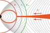 |
Fig. 1. Sketch of the disk and magnetic field configuration for an accreting system (not to scale). The truncation radius Rt indicates where the matter, indicated by the mass accretion rate Ṁ, couples to the magnetic field. The co-rotation radius where the magnetic field lines rotate at the same speed as the local Keplerian speed is at Rco. The outer radius, Rout, indicates the outermost radius where the central magnetic field is connected to the disk. Beyond this radius the stress becomes too large, causing the field to disconnect from the central source. |
A second important radius defines the region in the accretion flow where the plasma couples to the magnetic field. This region is usually defined as the volume where the energy density of the infalling plasma is smaller than the energy density of the magnetic field. The boundary where the energy densities are equal is called Alfvén surface (Alfvén & Lindblad 1947; Lamb et al. 1973). This surface has generally a complicated shape, depending on the structure of the surrounding plasma and the magnetic field. Its approximate shape is often derived by assuming a spherically symmetric plasma distribution that is only accelerated towards the gravitational center and by describing the central magnetic field with a dipole configuration with dipole moment μ. The field strength at point r is then given by
 (2)
(2)
where θ is the angle between r and the direction of the dipole moment (specifically, B = 2μ/r3 in the direction of the dipole moment). In this case the equilibrium condition gives the Alfvén radius
 (3)
(3)
where Ṁ is the mass accretion rate and where a term that depends on the angle between the dipole moment and the radius vector is ignored. The difference between RA and the true border of the Alfvén surface is at most a factor of 2 (e.g., Campbell 2018).
Note that the term Alfvén radius and its corresponding symbol are often used as a characteristic radius defining regions in the accretion flow as well as for the Alfvén surface (that is, the surface where the equilibrium condition is fulfilled), without a clear specification of any assumptions regarding the plasma and magnetic field. In this work we exclusively use it for the expression given in Eq. (3).
In all torque models we discuss in the following, it is furthermore assumed that a radius Rt exists at which the accretion disk is truncated because the matter is forced to follow the magnetic field lines. At this point the accretion flow transits from Kepler orbits to co-rotation and then falls along the magnetic field lines onto the surface of the accretor (see, Pringle & Rees 1972; Lamb et al. 1973; Basko & Sunyaev 1976; Ghosh et al. 1977; Popham & Narayan 1991). In the limit of a low magnetic field, where Rt is located at the surface or inside the accretor, angular momentum can be exchanged through friction, providing a limit to the angular momentum exchange (see, e.g., Frank et al. 2002, p. 153ff.; Syunyaev & Shakura 1986).
In the most simplified model for torqued compact objects it is assumed that the difference is fully transferred to the accretor (Pringle & Rees 1972; Ghosh & Lamb 1979). Describing the accretion disk with an α-disk model (Shakura & Sunyaev 1973), Ghosh & Lamb (1979) found that for Rt≪Rco the transition radius scales with the Alfvén radius, and that Rt/RA∼0.52 for typical NS accretors. Any difference of the angular momentum between the matter at Rt and at the surface of the compact object must be dissipated to enable accretion. Whether the total torque onto the accretor is positive or negative then depends on the interaction between the magnetic field and the accretion disk. Ghosh & Lamb (1979) assumed that a large part of the disk is linked to the accretor's magnetic field such that the part of the disk inside Rco, and therefore rotating faster than the field, exerts a positive torque on the central object. The part outside Rco, on the other hand, extracts torque from the accretor.
More recent models for torquing link the radius up to which the disk is connected, Rout, to the shear of the field inside the disk instead, no matter the exact location of Rt. This shear is commonly expressed as a function of the pitch angle of the field, up to a maximum allowed pitch that is related to the parameters of the disk's plasma (viscosity, diffusivity) and is generally assumed to be of order unity (see, e.g., Wang 1995; Matt & Pudritz 2005).
Numerical simulations have shown that the physical process of the coupling of the accretion flow to the magnetic field is more complex than the simple picture drawn so far (e.g., Romanova et al. 2008). Due to the coupling of the plasma at Rt a current is induced in the disk that causes a counter field opening up the magnetic field lines at Rt (i.e., Rout≈Rt). The central field and disk are therefore only barely directly connected. However, the opening of the field at Rt causes re-connections of the field, driving out plasma as magnetospheric ejections (e.g., Zanni & Ferreira 2013). These ejections are trapped in the sheath layer between the central field and the counter field of the disk. The field of the disk and the star are connected to the magnetospheric ejections, such that they provide an indirect link between the central field and the disk, resulting in an effective outer radius, Rout (Ireland et al. 2020, 2022)2.
In Sect. 3 we describe several analytical models and explicitly give the predicted torques. As discussed above, the spin-up due to accretion depends on the specific angular momentum at the inner disk edge of the disk, and therefore on the location of Rt, while the differential torque between disk and central field depends on the physics of the connected region. In all models we review the torque is derived from specific assumptions on Rt and Rco. Independent of the details of the specific model, the total torque exerted by the accreting matter on the central object can then be written as
 (4)
(4)
where τm is the contribution due to the magnetic interaction (differential rotation between disk and magnetic field) and where
 (5)
(5)
is the torque that corresponds to the angular momentum at Rt in the accretion disk plane (Ghosh & Lamb 1979). Elsner & Lamb (1977) showed that by factoring out τt the dimensionless function n defined in Eq. (4) only depends on one parameter, which is called the fastness
 (6)
(6)
where ΩK(r) is the Kepler orbit frequency at radius r:
 (7)
(7)
2.2. Dietary restrictions
Since the accretion behavior of NSs was discovered in the early 1970s, most observations of these sources were done during bright states, that is, at times of large mass accretion rates. It is important, however, to also consider accretion flow at lower mass accretion. Originally, it was believed that when not actively accreting, the fast rotating magnetic field of a NS prevents matter from getting closer than a certain radius (Illarionov & Sunyaev 1975; Campana 2001). This propeller state is believed to be entered when ω>1. Perna et al. (2006) showed with a simple ballistic calculation, not taking dissipative processes of plasma or gas dynamics into account, that one can obtain a critical radius, Rprop, and a corresponding fastness, ωprop, such that if Rt≳Rprop matter is ejected from the system. They also demonstrated that there is a truncation radius less than Rprop, corresponding, however, to ω>1, such that the matter is trapped between the gravitational potential and the rotating magnetic barrier. It is not clear if in this case accretion proceeds normally. There are arguments, however, that in this case the disk is truncated at Rco, accretion is greatly reduced and unstable (Rappaport et al. 2004; Romanova et al. 2008, 2018).
Three other aspects can also prevent matter from getting closer to the central object and under the influence of the magnetic field. Those are related each to a specific characteristic radius that gives the size of the accreting system. First, in wind-fed systems matter is efficiently accreted only if it is inside the accretion radius (often also called the gravitational capture radius)
 (8)
(8)
obtained from simple ballistic calculation of a particle with velocity v (e.g., Edgar 2004). The extent of the capture radius (subject to the wind properties) determines how much material is available for accretion.
Secondly, in fast-rotating pulsars with periods of milliseconds, typical for accreting millisecond pulsars (MSPs), a strong pulsar wind is produced by the rotating magnetic field. The characteristic radius determining the pulsar wind is the light cylinder
 (9)
(9)
where RS = 2GM/c2 is the Schwarzschild radius and c is the speed of light. During the accretion process the disk models are expected to hold with a reduced efficiency due to the pressure of the pulsar wind, up to a point where the pulsar wind can prevent accretion altogether (Shvartsman 1970; Parfrey et al. 2016).
Finally, we note that in addition to pressure due to the rotating magnetosphere, the static magnetic field pressure alone can (depending on the conditions of the plasma) also prevent or significantly reduce accretion (Toropina et al. 2003). This is particularly relevant for old neutron stars accreting from the interstellar medium (as opposed to a companion) but might also have an effect for wind accreting systems with conditions such that the ram pressure is relatively low. A review of the different stages for magneto-rotating accretors can be found in Lipunov (1987) and in Bozzo et al. (2008, however, see also Sokolova-Lapa 2023).
3. Different ways to connect plasma
From the previous description and assuming that the magnetic field structure is a dipole, Elsner & Lamb (1977) and Ghosh & Lamb (1979) established that episodes of stable accretion are only possible when ω<1, that is, Rt<Rco. The change in the angular frequency of the central object, dΩ, is related to the total torque via the change in angular momentum, dℒ, and moment of inertia, I:
 (10)
(10)
Here it is assumed that the moment of inertia is constant. Substituting the angular frequency with the spin period, P,
 (11)
(11)
where τ is expressed using Eq. (4) and  .
.
Equation (11) can then be used to estimate the total torque exerted on the central object provided measurements of P,  , and reasonable estimates of I. It is necessary to determine ω to calculate the change in the period. The fastness and n(ω) are tightly linked and therefore have to be determined together. In Sect. 3.2, we summarize and compare some of the common descriptions for this quantities.
3.1. One description to torque them all
Before we discuss specific model descriptions in Sect. 3.2, we have to address a subtle property of torquing models that complicates their interpretation. In general, torquing models can be roughly separated into two families: one where the approximation of Ghosh & Lamb (1979) is assumed to hold and a matching function n is constructed (e.g., Dai & Li 2006), and one where the plasma and magnetic field interaction and geometry is assumed from which n(ω), is derived (e.g., Wang 1995; Matt & Pudritz 2005). In the latter case, it turns out, that  (from Eq. (6) and Rt∝RA) does not hold in general as the approximation of Ghosh & Lamb (1979) is only valid in a small range and for ω≪1. Since the fastness is defined via the truncation and the co-rotation radii, it is an implicit function of the assumed magnetic field geometry and the coupling physics. This means that the fastness parameter depends on the specific assumptions of a given physical model. In particular, a value of ω is realized for different values of μ and Ṁ for different models. This degenerate situation makes it difficult to compare models when expressed as a function of ω only. For example, from the comparison of different n(ω) shown in Fig. 2 one could get the impression that the model of Ghosh & Lamb (1979) deviates significantly from the majority of other torquing models. As we shall show below, however, most of the deviation is due to the fact that ω has a specific meaning only within a given model. From here on ω will be replaced by ωi to reflect this in notation, where i is a label referring to a specific model
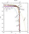 |
Fig. 2. Torque function, n(ω), as a function of the model-dependent fastness, ω, for the torque models discussed in Sect. 3.2. The dashed lines correspond to models where Rt∝RA is assumed. The red crosses show the values obtained by Ireland et al. (2020); the black circles are from Ireland et al. (2022) (see Table 1 for an explanation of the labels). As discussed in the text, no conclusions concerning the relative behavior of n(ω) between the different models should be drawn from this figure. |
In order to enable a direct comparison between different models, we therefore introduce a unifying description to treat all considered models in the same way, using well-defined physical quantities that are independent of the particular assumptions of the models. To this effect we introduce the canonical fastness
 (12)
(12)
and express all considered torque functions with this variable.
3.2. Model rundown
We now give an overview of several analytic torque models that have been proposed in the literature. The selection of the models does not aim for completion nor are any criteria applied, but it is based on an initial search for different approaches that all could be rewritten in a form using the unification as discussed above. In general, we give n(ωi) using a consistent notation and then show how the model-specific ωi can be derived for a given (model-independent)  . Table 1 gives an overview of the models addressed in the following. We note that several other models have been proposed that cannot be described easily in this way and therefore had to be excluded (see Sect. 5.4 for an example).
List of torque models and their symbols.
Probably the most influential model for torquing was described by Ghosh & Lamb (1979). As mentioned earlier, in the analytic form of the model Rt∝RA is adopted. Ghosh & Lamb assumed that the accretor's magnetic field causes a response field in part of the α-disk. Further assumption of the structure of this field led to an analytic approximation of the dimensionless torque function
 (13)
(13)
which is claimed to be valid for ω<0.9 (Ghosh & Lamb 1979, Eq. (10)). The restriction in ω here is only due to the approximation of the derived integral and not related to the estimate in the magnetospheric radius. The linear relation derived in the model is generally expressed as
 (14)
(14)
with Γ = 0.52 for Ghosh & Lamb (1979). While this directly allows one to express Rt=ΓRA, also called the magnetospheric radius, it will become clear that it is only valid in a narrow range.
Wang (1987) showed that the field configuration assumed by Ghosh & Lamb (1979) overestimated the toroidal magnetic field that can be supported by the plasma in the thin disk. Later, Wang (1995) derived three models based on different field configurations that are consistent with the plasma conditions of the thin disk. Assuming that the field is determined by re-connection at the Alfvén speed yields (Wang 1995, Eq. (9))
 (15)
(15)
Assuming that the growth of the magnetic field in the disk is limited by turbulent mixing gives (Wang 1995, see their Eq. 15)
 (16)
(16)
a result that was also obtained by Yi (1995) to explain the spin of T Tauri stars. Finally, the case that the magnetic field re-connection happens outside of the disk gives (Wang 1995, their Eq. (19))
 (17)
(17)
The response field in the disk is assumed to be the same in all three cases, while the timescale at which the internal field can react to external changes is derived for different characteristic velocities of the plasma (e.g., speed of sound).
For the configuration given by Wang (1995) together with the three characteristic velocities one finds the following implicit relations between  and ωi:
 (18)
(18)
Here all symbols are matched to the original description of Wang (1995), except for the variable Pz, that characterizes the pressure of the plasma at the truncation radius in units of the magnetic pressure perpendicular to the disk. Here, ξ≤1 is a fraction of the local Alfvén speed, γ≳1 characterizes how quickly the local velocity transitions from Keplerian rotation to co-rotation when leaving the disk plane, η≤1 is a screening coefficient of the field in the disk, α≤1 is similarly a scaling factor for the local sound speed, and γmax is the maximum pitch value that can be maintained.
Since the models of Wang (1995) and Ghosh & Lamb (1979) have a discontinuity at ωi = 1, they do not allow for a transition to the propeller state. Rappaport et al. (2004) argued that when Rt≳Rco the disk is not truncated further away, but instead the inner edge will be located at Rco. This argument is supported by numerical simulations (Romanova et al. 2008; Ireland et al. 2022) and in line with the arguments of Perna et al. (2006). Based on this assumption, Rappaport et al. (2004) constructed a model that extends the configuration described by Wang (1995). Effectively the model limits ωi≤1 with the extension that for Rt>Rco ωi = 1, such that Rappaport et al. (2004, their Eq. (23) & (24)) is rewritten as
 (19)
(19)
where
 (20)
(20)
It is important to note that for all models considered so far, a discontinuity is only reached if ωi can equal unity. Even the model of Wang (1995) has the property that ω→1 only for Ṁ → 0. Similarly, the full derivation of Ghosh & Lamb (1979) only approaches unity asymptotically. However, due to the approximations applied by Ghosh & Lamb (1979), which allowed them to derive analytic expressions, it appears as if ωi is unrestricted. As a results, the spin-down torque for high spin frequencies or low mass-accretion rates will be overestimated because ω should approach 1 only asymptotically. As discussed by Rappaport et al. (2004), their definition of ωi is based on setting Γ=(1/2)1/7 in Eq. (14). Note that the definition of the Alfvén radius by Rappaport et al. misses a factor of two in the denominator with respect to our definition in Eq. (3).
Another model using exactly the same concepts as the ones discussed up to this point was introduced for T Tauri stars (Matt & Pudritz 2005), where the magnetic field of a young star limits its maximum rotation rate. While the conditions in these systems are generally different from those in accreting neutron star systems, the accretion process is described by the same ideas. The model of Matt & Pudritz (2005) is parameterized in a way that determines the coupling strength between the disk and the magnetic field with two parameters. The inner connected region is determined by the maximum pitch angle, γc, that can be maintained for the lines connecting to the disk. A second parameter characterizes the diffusion of the plasma, β, and effectively models the coupling strength between the disk and the central field. Large values of γc permit more extended regions of the disk to be connected. From this, Matt & Pudritz (2005, Eq. (19) & (21)) derived a parametric torque function
 (21)
(21)
where ωp = 1+βγc. Due to the chosen parameterization, this model is able to reproduce most other models described here.
The defining equation for the fastness in the model of Matt & Pudritz (2005) can be written as
 (22)
(22)
where γ is again the magnetic pitch angle and β characterizes the coupling between the magnetic field and the disk, where small values indicate strong coupling.
By assuming that the magnetic configuration of Wang (1995) holds for all cases and that the torque is given from the Kepler orbits beyond Rco, Dai & Li (2006) made another attempt to allow transitions to ωi>1. For an arbitrarily chosen exponential transition function, they find (Dai & Li 2006, their Eq. (11))
 (23)
(23)
where ξ≲1 is a structure factor defining the torque at Rt and where γ is the limit of the magnetic field pitch at Rt. This is yet another model using the linear approximation (Eq. (14)), but this time with Γ = 1, that is,
 (24)
(24)
Combining the arguments of Rappaport et al. (2004) with the description of Wang (1995), Kluźniak & Rappaport (2007, their Eq. (36)) derived a torque function very similar to  :
:
 (25)
(25)
Importantly, based on the α-disk model, Kluźniak & Rappaport (2007) solved the disk structure for their assumptions as well as for the magnetic field configuration of Wang (1995). They also derived the torque based on the same assumptions as Wang (1995), therefore their second model,  , is equal to
  . The defining equations for the fastness are given by
 (26)
(26)
Concentrating on the strong magnetic fields present in ultra-luminous X-ray sources, Gao & Li (2021) extend the arguments of Wang (1987, 1995). Instead of assuming Keplerian motion at Rt, they propose a stiff disk model where the velocity at Rt matches the rotation velocity of the compact object (instead of the local Keplerian velocity). Otherwise following the same arguments of Wang (1995, for two of the three characteristic velocities given there) they find (Gao & Li 2021, Eq. (10) & (12))
 (27)
(27)
The fastness is implicitly given via
 (28)
(28)
where the parameters have the same meaning as for the model of Wang (1995).
3.3. Model comparison
Having expressed the torquing models in a uniform manner, we can now perform a comparison between them that is based on an identical meaning of the dynamical variable governing the torque,  . The relation between the model-dependent ωi and
  for all considered models is shown in Fig. 3. For models with additional parameters, we chose the default parameters by setting the additional model parameters to unity, with the exception of the model of Matt & Pudritz (2005) where β = 1 and γc→∞ (causing Rout→∞). The figure also includes results from Ireland et al. (2020, 2022) that have been obtained from numerical simulations of accreting T Tauri stars. In the T Tauri star community the disk-field interaction is invoked to explain the observed limit of the rotational period of the accretors that is much lower than what would theoretically be possible when considering only the amount of accreted matter with angular momentum given by Keplerian motion. The idea is that the connection of the central field to the disk causes currents in the disk that, in turn, create a magnetic field (Goodson et al. 1999; Goodson & Winglee 1999). At the boundary layer the magnetic field reconnects, trapping plasma from the disk. When the magnetic field is unloaded to release the stress it causes magnetospheric ejections (Zanni & Ferreira 2013). These magnetospheric ejections carry away large amounts of angular momentum and, thus, limit the maximum spin of the accretor.
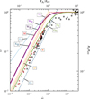 |
Fig. 3. Relation between the model-dependent fastness, ωi, and the canonical fastness, |

Except for the models shown with dashed lines, and from Kluźniak & Rappaport (2007), there are usually two to three parameters for each model that influence the detailed behavior and can essentially be referred back to the plasma parameters in the disk. Irrespective of the detailed behavior the global trend of  is always the same: For
  the fastness is a linear function, roughly matching the estimate from Ghosh & Lamb (1979), but often with an offset. For larger values, that is, lower mass accretion rates for a given spin frequency, the dependency changes and ωi approaches unity asymptotically. This fact seems to be often overlooked in the literature, given the number of models which extrapolate the linear relation to fast systems. Rather, for
  most models will lead to the truncation radius approaching Rco, matching the argument of Rappaport et al. (2004).
The resulting torque functions expressed as a function of the canonical fastness are shown in Fig. 4. The figure illustrates that, with the exception of the model of Rappaport et al. (2004), the different models are far more similar in behavior than one might have inferred from Fig. 2. Two quantities can be readily extracted from the models that show the remaining differences between them especially well: the maximum torque value possible and the equilibrium point, where n(ωi) = 0. Compared with the simulations of Ireland et al. (2020, 2022) it seems that most models drop off too quickly. This might be possible to resolve by employing different parameters for the magnetic interaction for the different models. What is striking is that the points of the simulation that are close to or beyond the equilibrium condition correspond to the points where the fastness deviates from the model predictions (dots in Fig. 4). It seems that the analytical models are no longer valid close and beyond the equilibrium point, that is, for spin-down. However, as said before, it is not clear whether the conditions of T Tauri stars are comparable to those in compact objects. Furthermore, the resulting torque from the simulations depends on how it is extracted from the results. Given the chaotic behavior at spin-down, this might introduce additional biases.
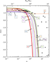 |
Fig. 4. Torque function of all considered models expressed via the canonical fastness. The labels indicate the models with the corresponding subscript. The dashed lines indicate models where Rt∝RA. The red crosses mark the results of Ireland et al. (2020) and the black circles that of Ireland et al. (2022). The black circles with a dot identify the simulations in the transition region of Fig. 3, with 0.6<ωi<0.8. |
It is also noteworthy that the simulations have a maximum torque value at ωi→0 that exceeds the analytical models, except for the expressions of Matt & Pudritz (2005) and Gao & Li (2021). The reason is the assumed velocity at Rt. In most models it is assumed that up to this radius, the disk is described by Keplerian motion, while for nG it is assumed that the velocity at the inner edge of the disk matches that of the rotating magnetic field. A special case is the model of Matt & Pudritz (2005), where the coupling between the disk and the field are subject to the value of ωp. This behavior also influences how strongly the plasma is forced to follow the field. For smaller values the disk experiences more drag, specifically for ωp = 2,  . The other solution,
  , is approximately reproduced by nM for
  . Due to the branch for the critical fastness, ωc, a somewhat similar behavior to the Wang (1995) models can be achieved, however, with a constant spin-up below the critical fastness and a sharper drop off above.
3.4. Torquing neutron stars: Predicting spin changes
Having established the different values for the torque, we can now compute how the accretion flow changes the spin of the neutron star. The torque relation (Eq. (11)) connects the spin period and its derivative with the system parameters (magnetic field, mass, distance, and spin period) and the mass accretion rate. As the latter cannot be observed directly, it is commonly assumed that it correlates with the X-ray luminosity of accreting systems (Zel’dovich & Novikov 1966; Shklovsky 1967). Assuming that the potential energy of the infalling matter is converted to photons with X-ray luminosity
 (29)
(29)
where ɛ≤1 is the conversion efficiency3, R the radius of the accretor, and M its mass. The luminosity is obtained from the observed flux, F, by
 (30)
(30)
where D is the source distance and α is a parameter depending on the emission characteristic. For isotropic emission α = 4π. Using Eq. (5), (29), and (30), and expressing the moment of inertia via the dimensionless radius of gyration, k,
 (31)
(31)
we obtain
 (32)
(32)
where h=ɛ/α, while the definition of the fastness and the canonical fastness yield
 (33)
(33)
Combining this equation and Eq. (3) we can finally write
 (34)
(34)
where we introduced two auxiliary parameters, the effective pole strength  ,
,
 (35)
(35)
and the coupling strength ℬ,
 (36)
(36)
which summarize the system parameters.
Combining the conversion factor, ɛ, and the emission characteristic, α, into the weighted efficiency, h, expresses our ignorance towards the relation between accreted matter and photons reaching the observer, including the limited energy range of the instruments. Generally h is time dependent, but often assumed to be constant for simplicity. We expect that deviations from constancy are mainly influenced by long term trends in the emission characteristic, that is, changes in α. The shift of maximum emission relative to the energy band used to measure L is reflected by changes in ɛ. Finally, an effect that seems often ignored when torque models are applied to data obtained from neutron stars is that when the mass-accretion rate is calculated based on the observed flux, the gravitational red-shift must be taken into account, since the flux observed differs from the emitted flux in the frame of rest of the neutron star by a factor between 1.6 and 2.4. In our notation this correction is implicitly taken into account through the value of h.
The particular separation into the two auxiliary variables is done such that the canonical fastness is only dependent on one of those parameters
 (37)
(37)
In this form the model can be directly compared with data consisting of the time-dependent flux, F, and spin period, P. The differential equation (34) can be solved by standard numerical integration. With a particular choice of the torque function ni(ωi) and corresponding relation between  and ωi the model can be fitted to the data.
3.5. Equilibrium fastness
Given all models above we can immediately calculate the equilibrium point, ωeq, where n(ωeq) = 0. If a source is accreting constantly the equilibrium value corresponds to a spin period Peq that should be reached after some time, and here the central accreting object is neither spinning up nor down. This value is often used to estimate system parameters as it is expected that persistent sources accrete roughly with a constant rate. For this reason we give the equilibrium fastness for all models in Table 2. To visualize how the equilibrium location changes for the parameters for the models of Matt & Pudritz (2005) and Dai & Li (2006) with respect to the other models, Fig. 5 shows the values for different parameter combinations, where the x-axis is ωp for nM and ξ/γc for nD. As for the torque function, comparison between different models for a particular system must be done via  .
.
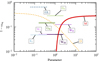 |
Fig. 5. Visual representation of the equilibrium fastness. The parameter is either ωp for Matt & Pudritz (2005) or ξ/γc for Dai & Li (2006). For ωp the lower bound is 1. All other models have fixed values for the equilibrium fastness (see Table 2) and are displayed over an arbitrary short range for clarity only. The dashed lines indicate models where Rt∝RA. |
Resulting equilibrium fastness values, ωeq.
One important factor of the equilibrium fastness is to understand how it connects to a potential equilibrium period. The latter is often used as an estimate for persistently accreting systems. However, the equilibrium fastness only directly translates into an equilibrium period if the mass accretion rate is constant. More generally, however, the mass accretion rate can often be approximated by a stochastic process, potentially with a constant mean accretion rate. Depending on the exact parameters of the system, this stochastic process can lead to a drift of the period instead of to a system in equilibrium, even if the average mass accretion rate is constant. As a simple demonstration, Fig. 6 shows how the period of a neutron star is predicted to change with time for the different torquing models. Despite the fact that the average mass accretion rate is constant in the Poisson process assumed here, and despite the fact that the starting period was set to match the equilibrium period for that mass accretion rate, the period of the neutron star is predicted to vary with time.
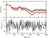 |
Fig. 6. Top panel: Predicted change in rotation period for all models (except Rappaport et al. 2004) for a given starting period and a mass accretion rate defined by a Poisson process. The colors indicate the models, as before. The dashed lines indicate models with Rt∝RA. Bottom panel: Simulated Poisson light curve. |
4. Application to the Be X-ray binary 4U 0115+63
We now apply torquing theory to a real observational example, in order to illustrate how they can be used to estimate system parameters and in order to reveal some of the typical problems that can occur using torque models. Specifically, we consider the four observed outbursts of the Be binary system 4U 0115+63 (Giacconi et al. 1972; Bissinger et al. 2020, and references therein) captured by the Fermi gamma-ray burst monitor4 (GBM, Meegan et al. 2009) and the Swift burst alert telescope5 (BAT, Gehrels et al. 2004, 2005). This source is very well known because of its multiple CRSFs in the X-ray spectra, which allow the accurate measurement of the magnetic field strength (Wheaton et al. 1979; Santangelo et al. 1999). The discussion here is only to showcase the performance of the models in comparison to each other and should not be understood as an in-depth analysis of the system. In addition to the direct measurement of the magnetic field in 4U 0115 through cyclotron line measurements, being a Be-binary system with several bright outbursts, the source shows a very clear spin-up signal linked to the large dynamic range in mass accretion rate. In comparison, more classically viewed disk accretion systems like Vela X-1 or Cen X-3 are close to the spin equilibrium and the accretion is therefore more chaotic causing some disconnection between the spin and luminosity signal. As we illustrated in Sect. 3 it should be clear that the prediction for spin-down is much less understood which would complicate the comparison even more.
Before attempting to combine the light curve, the observed evolution of the spin period, and a specific torque model, we can perform expectation management based on the expression given in Eq. (34). Generally, for accreting highly magnetized neutron stars, we can assume that the mass, radius, moment of inertia, and magnetic field of the accreting object are constant in time due to the overall small accreted mass and the timescales considered here. With this in mind, the only remaining time dependence in the parameters is the conversion efficiency and the emission characteristic in ℬ. Without further information on the flux, we assume that h is constant on timescales much larger than the pulse period. This leaves us with a total of five parameters, one  , and four ℬ's.
4.1. Confronting reality
In order to obtain the mass accretion rate from the observed light curve, a conversion of the instrument specific count rate to luminosity is necessary. If broadband spectral coverage is available, the luminosity can be determined from the measured flux by assuming a certain emission characteristic. Here we simply assume that this conversion factor is constant over each outburst, it can therefore be seen as an additional contribution to h. For an unconstrained parameter search, we make no assumptions on the distance and determine the value of ℬ directly from the data.
Equation (34) directly shows that there is a parameter correlation between  and ℬ when model fitting. Given that for slow rotators n tends towards a constant value, it is nearly impossible to disentangle the two parameters without additional information. Strong correlation between parameters poses a challenging problem for most fit methods. For this reason it is better to treat the ratio
  as one parameter. But even with this modification a correlation between the parameters remains, since for larger values of ℬ the canonical fastness will increase. This, in turn, reduces the spin-up and increases
  . Only the transition to spin-down at even larger values of ℬ limits the range of the parameters. Overall, it should therefore be expected that a large systematic uncertainty will be present in all fit results, introduced by the conversion from light curve to mass accretion rate. An unconstrained parameter search will thus most likely never result in specific estimates for the magnetic field or distance but only a relation between those two quantities.
Another factor complicates the matter: Binary motion. Be X-ray binaries have typical orbital periods of 10–1000 days (Malacaria et al. 2020). In some systems regular type I outbursts can be observed tightly linked to the orbital period, that last only a fraction of the orbit. More luminous type II outbursts are observed rarely and less connected with the orbital period, and can last over serval period cycles (Reig 2011). Especially for the latter the measured spin period is affected by the Doppler shift due to the orbital motion. To predict the change in spin period the mass accretion rate at the rest frame of the accretor must be determined. To convert the flux from the observer frame to the rest frame a solution for the orbit must be found. Unless the orbit is well known from other measurements, the best way to achieve this is by fitting the orbital parameters simultaneously to the torque function. The full model is then written as
 (38)
(38)
where T is the solution of Eq. (34) with integration constant P0, D is the Doppler correction of the intrinsic period due to orbital motion, and the connection between tobs and trest is obtained from the light travel time of the orbit solution. For many objects the orbital parameters are not sufficiently well determined to allow a correction up front. Therefore, applying the orbit as part of the model is necessary and also allows a potential time dependence of the orbital elements to be measured.
4.2. Torquing results
We show the light curve of 4U 0115+63 as monitored by Swift/BAT in Fig. 7, together with the spin period as measured by Fermi/GBM. Only the relevant time spans of bright phases are shown. Wang (1995) argue that their model III should describe the scenario of an accreting Be X-ray binary. The resulting best fit of this model modified by the Doppler effect is shown in red, the intrinsic spin-up is shown in green. We ignored several data points from the Fermi/GBM data, mainly because they are at the edge of the intervals covered by Swift/BAT. The first few data points taken during the outburst of 2011 are ignored because of the missing light curve information in between. We also ignored the three outliers in the Swift/BAT data of the 2023 outburst.
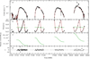 |
Fig. 7. Torque modeling for 4U 0115+63. (a) Light curve of 4U 0115+63 as measured by Swift/BAT. The red curve is the interpolation of the data. (b) Pulsation period as measured by Fermi/GBM. The red curve is the best-fit model of WIII modified by the Doppler shift of the orbit. The green curve is the intrinsic spin-up of the NS. (c) Intrinsic spin-up signal predicted by the model (same as the green curve in panel (b). (d) χ residuals of the spin model. For all panels, the crosses enclosed by gray diamonds have been ignored for the model comparison; we also note the gaps on the time axis. |
Despite showing only the model of Wang (1995), we applied all discussed models to the data in the same way. Without constraining the magnetic field, all models fit the data very well, and to an extent that no favorable model can be chosen.
To get a better understanding of the correlation between the parameters we explored the statistics landscape of the parameter space with the method proposed by Foreman-Mackey et al. (2013). For all four outbursts this revealed the already expected nearly linear correlation between  and ℬ. Furthermore, the orbital parameters showed a correlation with the torque parameters. While the resulting orbital parameters are hardly affected, it appears that the torque parameters are more sensitive to the additional degrees of freedom. To some extent this is expected as the impact of the orbit on the signal is much larger than the impact of the spin up. Some results of the parameters space exploration are shown in Appendix A.
From the distribution of the resulting torque parameters we can estimate the distribution of the surface magnetic field at the pole via  . Assuming canonical values M = 1.4 M⊙ and R = 106 cm we obtain the magnetic field distributions for all models and outbursts (Fig. 8). These distributions show clearly that any magnetic field estimate that is based on torque theory is not well constrained for a single model, and that magnetic field strength estimates vary widely between different models. In addition, the estimate suffers from a systematic uncertainty due to variations in the plasma parameters. As such, it seems a far stretch to get reliable values for the dipole moment. One might be tempted to argue that this is only the case for our specific example, because no information of the distance or the conversion factor is taken into account. However, as is clear from the parameter dependencies, knowledge of this information helps only if the emission characteristic and conversion efficiency, h, are known too, which in general is not the case.
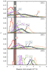 |
Fig. 8. Marginal probability distribution of the pole magnetic field strength estimated for all considered models. The colors indicate the identifier of the model. The dashed lines correspond to models with Rt∝RA. The gray area indicates the value range estimated from the CRSF features. |
Torque models are often also used to measure the distance of a source. Using parameter distributions we find that the distance distribution between the outbursts is indeed very similar. However, different models also give different estimates. Especially models where Rt∝RA consistently yield the largest distances. This can be explained due to the fast transition to spin-down present in these models. Generally these models require a smaller ℬ to describe the data, resulting in a larger distance for the same  .
.
The surface magnetic field of 4U 0115+63, as estimated from cyclotron line measurements (Bissinger et al. 2020, for example) is 1–1.4×10¹² G (depending on the assumed gravitational redshift). In principle we can use these values to judge the performance of torque models to estimate magnetic field values. From the distribution of the best-fit magnetic fields shown in Fig. 8 it seems that the models group into three classes. The lowest field estimates are generally given by the model of Matt & Pudritz (2005) and very similar by that of Dai & Li (2006). Slightly larger values are obtained with the prescriptions of Ghosh & Lamb (1979) and the first and second model of Wang (1995). The largest estimates, and also the least constrained ones, are obtained based on Kluźniak & Rappaport (2007) and Gao & Li (2021). The ad-hoc solution given by Rappaport et al. (2004) shows very clearly the effect of the artificial fix point resulting in a discontinuity in the torque function. In conclusion, while all models (except Rappaport et al. 2004) yield values in the ballpark of the cyclotron line results, it seems that the third class of models favors larger values. In comparison with the value obtained through cyclotron line measurements we find a first indication what torque models perform better. However, it seems that at least some models result in B-field estimates which are not compatible between the outbursts, which lets us conclude that those are affected by systematic uncertainties. Because it is not clear how comparable the local magnetic field strength in the cyclotron line forming region is with the value inferred from the large-scale dipole field it is difficult to choose any one model over the others here. Such a choice can only be made based on the application of the models to a large sample of outbursts of different sources.
4.3. Time dependence of magnetospheric radius
From the determined fastness of the system we can also readily calculate the expected location of the inner edge of the accretion disk. In Fig. 9 we show the truncation radius for all models over the outbursts, derived from the unconstrained best-fit solution with canonical parameters M = 1.4 M⊙ and R = 106 cm. The figure also explains why the resulting magnetic field distribution for the model of Rappaport et al. (2004) discussed above has sharp edges: The fix-point at ω = 1 introduces sharp transitions in the truncation radius and are therefore likely not well explored by the MCMC method. For the other models, the absolute position of the truncation radius varies in accordance to the hierarchy classes for the magnetic field estimates. From the resulting distributions of the magnetic field (Fig. 8), it is evident that even the same models give different results for the magnetic field for different outbursts. As it is not expected that the large-scale magnetic field changes significantly over the observed time span, this is likely an artifact of the model approach in general. One contribution certainly can be attributed to the model for the orbit as it is to some extent in conflict with the torque model. This is manifest in the slight variation of the measured orbital parameters (see Appendix A).
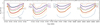 |
Fig. 9. Time dependence of the truncation radius for the unconstrained best fits for each model. The labels indicate the model corresponding to the predicted truncation radius. The dashed lines indicate models with Rt∝RA. The dotted black line marks the radius of co-rotation. |
A factor that needs to be considered is the quality of the data. The measurement density of the spin period as well as of the light curve drive the result. This is most noticeable in the data for the 2023 outburst where nominally the magnetic field is most constrained. However, this is only because the models overall do not fit the data very well. The detailed interplay between the data quality and applicability need to be studied further to resolve those problems.
5. Other aspects of accretion and angular momentum change
All of the models considered here are based on simplifying assumptions that are likely not realized in reality. First and foremost, all models assume that accretion happens via a Keplerian disk with the angular momentum aligned with the rotation axis and the magnetic dipole axis of the accretor. For a more realistic picture, where at least one of those symmetries are broken, additional effects of the disk-field interaction might become relevant. Systems where accretion does not happen via a disk might have very different behavior than predicted from the torque models above which leads to further uncertainty in the measurements. Especially relevant for evolutionary studies are other mechanisms that change the angular momentum of the accretor. In this section we mention some of the undertaken efforts that have been done to estimate effects due to additional interactions or geometries, all of which are necessary to understand for a more unified picture of the spin evolution of compact accretors.
5.1. Inclination of magnetic axis
The highly symmetric case of the “aligned rotator” simplifies calculations, but is also very unlikely to occur in reality. For an accreting neutron star it would not even be consistent with pulsed emission that allows us to measure the spin period. Without changing the overall arguments for the accretion process one can consider an inclined magnetic axis. In polar coordinates (r,ϕ), the magnetic field in the disk plane for an inclined dipole is given by (e.g., Jetzer et al. 1998)
 (39)
(39)
with the inclination angle χ. With this the truncation radius is (Jetzer et al. 1998; Perna et al. 2006)
 (40)
(40)
To first approximation the modification of the radius can be applied to the Alfvén radius and the truncation radius is obtained for this modified RA now dependent on ϕ. As a consequence one finds that the truncation radius is at varying distance to the co-rotation radius around the disk. From this it is expected that the plasma has a different angular momentum depending on ϕ. To get the total torque on the central object one therefore has to integrate over ϕ taking this variation into account.
5.2. Mass pileup at magnetosphere
Similar to the ϕ dependence of the magnetosphere, the general torque will also depend on the structure of the disk at the truncation radius in z direction, that is, the height above the accretion disk. The influence of this is explored by Eksi & Kutlu (2011) and Çıkıntoğlu & Ekşi (2023) based on its influence on the mass flow rate. These authors argue that the magnetic field prevents matter from accreting in the disk plane because there the plasma is forced to move in the z direction. Therefore the plasma piles up towards larger z until it reaches a point where it can penetrate the field. This behavior has two consequences: first, it modifies the inferred mass accretion rate at the magnetosphere from the luminosity, and second, it introduces a natural asymmetry in the transition from inhibited accretion to accretion and vice versa.
The key property that drives the evolution here is where the magnetospheric boundary crosses the equilibrium surface. This surface is defined by the equality of apparent acceleration due to the centrifugal effect and the gravitational force along the magnetic field lines. If at some distance Rt crosses inside the equilibrium surface matter can penetrate and is accreted from above the crossing point. If the surfaces do not cross, accretion is inhibited, leading to the propeller state.
5.3. Propeller state
To explain the synchronous orbits and periods of close X-ray binaries, Davidson & Ostriker (1973) introduced the concept of an equilibrium period controlled by a centrifugal barrier possibly flinging material out of the system. Later, and introducing the term propeller state, Illarionov & Sunyaev (1975) used this accretion regime to explain the low number of observed accreting neutron stars. The conceptual idea is simple: If the accreted material couples to the magnetosphere at a distance that is larger than the co-rotation radius, the matter is accelerated onto trajectories that correspond to orbits with increasing radius (where Rt is the closest point). Therefore, for sufficiently extended magnetospheres matter will be pushed out of the system and not accreted.
There is, however, a possible accretion regime where the centrifugal effect does not permit accretion onto the compact object nor does it provide enough momentum for the matter to leave the gravitational potential. A simple ballistic argument gives a quantitative range for the relevant radii for where this trapping state should occur (Perna et al. 2006). In both cases angular momentum is removed from the central object and converted either into momentum of the gas outflow or convective motion.
The disk accretion models discussed above do not include the transition from accretion over the trapped state to the propeller. The quantification of the magnetosphere in those models via the mass accretion rate introduces an artifact for this transition. We like to remind that the magnetosphere is formally defined by the energy density balance between the gas and the magnetic field. The energy density of the gas can be expressed via its pressure, which in turn can be formally expressed by the accretion rate. The pressure inward, however, is counteracted by the pressure of the magnetic field. In the propeller state the accretion rate is necessarily zero, as is the total pressure at the magnetosphere. The pressure of the gas that determines the location of the magnetosphere, however, is finite (Shakura et al. 2012).
5.4. (Quasi-)spherical accretion
While the formation of an accretion disk is a very universal phenomenon in astrophysical objects where the accreted flow has a specific angular momentum, in binary systems where the donor star has a strong a stellar wind with high velocity it is expected that instead a shell of plasma forms around the accretor. Shakura et al. (2012) explored the case for subsonic quasi-spherical accretion, extending the discussion of Davidson & Ostriker (1973) and Illarionov & Sunyaev (1975). With otherwise very similar arguments compared to the disk case, Shakura et al. find that the magnetosphere scales differently with the mass accretion rate compared to the disk models. In this model the wind and the angular momentum of the plasma shell are formulated via the orbital parameters with the wind velocity expressed as a function of the separation of the two bodies. As a consequence the model intrinsically depends on the orbital separation and orbital period, compared to the added modulation due to observer effects (see Sect. 4).
The focus of the model of spherical accretion is the magnetospheric boundary for a plasma shell. The dispersion velocity of the plasma at the boundary is investigated to calculate an approximation of Rt (labeled RA by Shakura et al. 2012). The solution is then written with a numerical factor, f(u), that quantifies the dispersion velocity via the free-fall velocity at Rt. The resulting relation between Rt and RA then depends on  . This additional factor prevents us from rewriting this model solely as a function of the fastness and canonical fastness.
It should be noted, however, that the expression of the model by Shakura et al. (2012) is derived based on a linear approximation of f(u). This approximation improves for Ṁ → 0. On the other hand, f(u) must be <1, which is not automatically guaranteed in the linearized formulation of the model. In a way, this is a similar problem to the disk models given above for ω→1.
5.5. Super-Eddington accretion
Another modification of the torque models happens for extremely large mass accretion rates. These accretion regimes have gained a lot of attention with the discovery of the first pulsating ultra-luminous x-ray source (Bachetti et al. 2014). These sources are interesting for a number of reasons and would benefit significantly if torquing can provide an estimate of the magnetic field of the accretor. Due to the large amounts of matter that fall towards the compact object the disk is no longer gas-pressure dominated but by the radiation pressure. This causes a change in the disc structure, increasing its height significantly (e.g., Chashkina et al. 2017; Mushtukov et al. 2019). This change also affects the coupling between the matter and the magnetic field such that the magnetospheric radius is altered (Chashkina et al. 2019).
From the theoretical descriptions of the change with increasing accretion rate an effective model was constructed and applied to the galactic pulsating ultra-luminous x-ray source Swift J0243.6+6124 (Kennea et al. 2017; Jenke & Wilson-Hodge 2017). It was found that the predicted effect for high accretion rates is clearly visible in the data and that a model that takes this change into account is favored over a model with Rt∼RA (Karaferias et al. 2023). This change can be interpreted as a change from a disk accreting state to one that corresponds to spherical accretion.
5.6. Transition between accretion regimes
In highly magnetized neutron star binaries it is suspected that during an outburst some system undergo a transition from the propeller state to the accretion state. From the asymptotic behavior of all of the discussed torque models at ω = 1 (except Rappaport et al. 2004), it is clear that they do not work for this transition. A general description of this transition has not yet been made, however, an attempt to connect different accretion regimes by simple arguments was given by Ertan (2020). The main argument here is that the solution for the magnetospheric radius should also hold for ω>1. This solution branch can be obtained for all models where Rt is derived from the equilibrium condition6. In the equilibrium condition only the absolute value of ω−1 is meaningful, and therefore replacing it with |ω−1| allows one to obtain the second solution for ω>1. The difference of the model of Ertan (2020) is that there are two distinct solutions in the range for ω<1 and only one for ω>1 while the situation is reversed for all models considered in our work.
Ertan (2020) further argue that the second solution is only valid for the case where matter can be effectively removed from the system. They chose a ballistic solution similar to that obtained by Perna et al. (2006) as the transition point (Rt>21/3Rco). For smaller truncation radii, but still with ω>1, they assume that truncation happens at Rco (Rappaport et al. 2004). To connect the two branches, Ertan choose to intersect the truncation radius with the linear solution of Ghosh & Lamb (1979) for a parametric scaling factor. This approach, while not rigorous, allows one to investigate full evolutionary tracks of accreting objects given initial parameters and mass accretion and the influence of the various regimes.
5.7. Additional loss of angular momentum
In addition to the torque exchange through the linked disk there are other contributions relevant for the spin evolution of a compact object. For radio pulsars angular momentum is extracted by the pulsar wind, caused by the rotating magnetic field, which steadily slows the rotation (Pacini 1967; Gold 1968; Goldreich & Julian 1969). For accreting millisecond pulsars, Parfrey et al. (2016) derived a toy model, taking the disk-field interaction as well as the pulsar wind into account. The characteristic scale for this model is given by the light-cylinder, Rlc, which introduces an absolute value for the characteristic radii. Due to this change of scale, the description via the fastness contains an additional dependency on the rotation period and can no longer be described via ω or  .
.
6. Conclusion
In this paper we showed that it is possible to express most models for the torque exerted onto a neutron star by its accretion flow in terms of one physical quantity, the canonical fastness,  . Using this quantity ensures that the models are expressed with one set of physical quantities. Using
  , it is possible to directly compare many of the torque models in the literature, while comparing them using the model-dependent truncation radius hides the fact that the same truncation radius is realized for incompatible accretion scenarios (Ṁ, μ). We showed that the models generally follow similar trends and are much more similar than is typically assumed when comparing their behavior using the model-dependent fastness, ω. We then developed a general torquing formalism, showing that it is possible to describe many of the proposed simplified disk torque models with two parameters,
  and ℬ, that can be related to the physical parameters of the accreting system.
Despite the simplicity of the models, they are very successful in describing the observed data of the Be X-ray binary system 4U 0115+63. The predicted system parameters, however, are far from consistent between outbursts, even when applying the same model. Considering that different and equally valid torquing parameterizations give results ranging over one order of magnitude, and given that no model yields parameters that are clearly statistically preferred argues against using torque models to derive reliable physical properties of neutron stars at this stage. In particular, the derived magnetic field strength ranges over one order of magnitude between models, even without accounting for the systematic uncertainty in the interaction parameters, which would increase the uncertainty of the model parameters even more. As an example, for the Galactic ultra-luminous x-ray pulsar Swift J0243.6+6124 (Kong et al. 2022) argue that the magnetic field inferred from its cyclotron line, B≈1.6×10¹³ G is in contradiction with the results from magnetic field estimates based on torque theory (e.g., Jaisawal et al. 2019). However, given the extreme Ṁ of this source, in combination with a large B-field strength, estimated from cyclotron line measurements, the system should be considered fast. This is exactly the range that is affected most strongly by the linear approximation of Ghosh & Lamb (1979), making torque theory unreliable. In a similar fashion, in their simplified form torquing models are generally not consistent with other methods estimating the extent of the magnetosphere (Bozzo et al. 2009).
Despite their shortcomings, however, these simplified torquing models are still useful in order to understand the general trends of the spin period for disk accretors, linking Ṁ to the spin period. With the latter being much better constrained by observations and combining this with physical spectral models, it might be possible to invert the problem. By this we mean that instead of using the mass accretion rate (inferred from the light curve) as input, one could use the observed pulse period as a proxy for the mass accretion rate parameter used by some physical accretion models (such as Becker & Wolff 2007; Sokolova-Lapa et al. 2021). The drawback of this approach is that it requires access to a number of high quality broadband X-ray spectra covering a large part of an outburst, which might not be easy to obtain.
A systematic study of proposed torque models and their application to the rich dataset observed by individual observer campaigns and monitoring programs such as BATSE (Bildsten et al. 1997) and Fermi/GBM (Malacaria et al. 2020) will allow us to understand and correct for the systematics in the analytical torque models. The comparison with data and also with numerical simulations might provide a way to connect the accretion process to the low luminosity or propeller state. As mentioned before, at low Ṁ the luminosity is no longer a good proxy for Ṁ because it appears only formally in the equations, representing the pressure at Rt. In the transition to a non-accreting regime, Ṁ approaches zero while the pressure stays finite. Solving this problem in the torque models can provide additional constraints to understanding systematic deviations.
Given the simplicity of most torquing models it is not particularly surprising that the results are inconsistent or biased. Even so, identifying a model that at least approximately yields somewhat trustworthy magnetic field estimates would be very useful in order to compare different accretors and their accretion stages. In the particular case of 4U0115+63 discussed here, at least order of magnitude estimates seem to be consistent with cyclotron line measurements. Understanding whether this holds in general could be achieved by a broader study of CSRF sources, describing their pulse period evolution with different torquing models, and then identifying the model that is most consistent with the magnetic field determined from cyclotron lines. There are several caveats, though. First, it is not clear whether the CSRF forming region is a good representation of the large-scale magnetic field. In addition, different sources might be best described by different torquing models.
To conclude, it appears that applications of torque theory in order to estimate the magnetic field of accreting neutron stars are more strongly affected by systematic uncertainties than generally acknowledged in the literature. Torquing theory can explain general trends in the pulse period behavior, but in its current state it is unreliable and does not yield precise numbers.
Acknowledgments
This research was supported by the International Space Science Institute (ISSI) in Bern, through ISSI International Team project #495 (Feeding the spinning top). GV acknowledges support from the Hellenic Foundation for Research and Innovation (H.F.R.I.) through the project ASTRAPE (Project ID 7802). CM acknowledges funding from the Italian Ministry of University and Research (MUR), PRIN 2020 (prot. 2020BRP57Z) “Gravitational and Electro magnetic-wave Sources in the Universe with current and next generation detectors (GEMS)” and the INAF Research Grant Uncovering the optical beat of the fastest magnetised neutron stars (FANS). IEM acknowledges funding via the BASAL Centro de Excelencia en Astrofisica y Tecnologias Afines (CATA) grant PFB06/2007. JW and ESL acknowledge support from Deutsche Forschungsgemeinschaft grant WI 1860/11-2.
For accretion flows around black holes, the magnetic field advected inwards by the accreted material can also reach values that are high enough that it plays an important role in the flow dynamics (Uzdensky 2004, 2005; Nathanail & Contopoulos 2014), but we exclude these effects in this paper.
The MHD simulations cited here were conducted in the context of T Tauri stars. These have central magnetic fields several orders of magnitude lower than accreting neutron stars. Nevertheless, it is expected that the magnetic field at Rt acts mostly as a scaling factor and so overall the results should still hold.
The conversion efficiency, ɛ, is commonly set to 1 for accreting neutron stars.
Ertan (2020) derive their own estimate for Rt in a way that does not allow for a description via ω and  .
.
References
- Alfvén, H., & Lindblad, B. 1947, MNRAS, 107, 211 [CrossRef] [Google Scholar]
- Bachetti, M., Harrison, F. A., Walton, D. J., et al. 2014, Nature, 514, 202 [NASA ADS] [CrossRef] [Google Scholar]
- Basko, M. M., & Sunyaev, R. A. 1976, Sov. Astron., 20, 537 [Google Scholar]
- Becker, P. A., & Wolff, M. T. 2007, ApJ, 654, 435 [NASA ADS] [CrossRef] [Google Scholar]
- Becker, P. A., Klochkov, D., Schönherr, G., et al. 2012, A&A, 544, A123 [NASA ADS] [CrossRef] [EDP Sciences] [Google Scholar]
- Bildsten, L., Chakrabarty, D., Chiu, J., et al. 1997, ApJS, 113, 367 [CrossRef] [Google Scholar]
- Bissinger, K. M., Kreykenbohm, I., Ferrigno, C., et al. 2020, A&A, 634, A99 [NASA ADS] [CrossRef] [EDP Sciences] [Google Scholar]
- Blondin, J. M. 2013, ApJ, 767, 135 [Google Scholar]
- Bondi, H., & Hoyle, F. 1944, MNRAS, 104, 273 [Google Scholar]
- Bozzo, E., Falanga, M., & Stella, L. 2008, ApJ, 683, 1031 [Google Scholar]
- Bozzo, E., Stella, L., Vietri, M., & Ghosh, P. 2009, A&A, 493, 809 [NASA ADS] [CrossRef] [EDP Sciences] [Google Scholar]
- Campana, S. 2001, AIP Conf. Proc., 599, 63 [Google Scholar]
- Campbell, C. G. 2018, Magnetohydrodynamics in Binary Stars (Springer) [CrossRef] [Google Scholar]
- Çıkıntoğlu, S., & Ekşi, K. Y. 2023, MNRAS, 524, 1727 [Google Scholar]
- Chashkina, A., Abolmasov, P., & Poutanen, J. 2017, MNRAS, 470, 2799 [Google Scholar]
- Chashkina, A., Lipunova, G., Abolmasov, P., & Poutanen, J. 2019, A&A, 626, A18 [NASA ADS] [CrossRef] [EDP Sciences] [Google Scholar]
- Cropper, M. 1990, Space Sci. Rev., 54, 195 [CrossRef] [Google Scholar]
- Dai, H. -L., & Li, X. -D. 2006, A&A, 451, 581 [NASA ADS] [CrossRef] [EDP Sciences] [Google Scholar]
- Davidson, K., & Ostriker, J. P. 1973, ApJ, 179, 585 [NASA ADS] [CrossRef] [Google Scholar]
- Edgar, R. 2004, New Astron. Rev., 48, 843 [CrossRef] [Google Scholar]
- Eksi, K. Y., & Kutlu, E. 2011, AIP Conf. Proc., 1379, 156 [Google Scholar]
- El Mellah, I., Sander, A. A. C., Sundqvist, J. O., & Keppens, R. 2019a, A&A, 622, A189 [NASA ADS] [CrossRef] [EDP Sciences] [Google Scholar]
- El Mellah, I., Sundqvist, J. O., & Keppens, R. 2019b, A&A, 622, L3 [NASA ADS] [CrossRef] [EDP Sciences] [Google Scholar]
- Elsner, R. F., & Lamb, F. K. 1977, ApJ, 215, 897 [NASA ADS] [CrossRef] [Google Scholar]
- Ertan, Ü. 2020, MNRAS, 500, 2928 [CrossRef] [Google Scholar]
- Farinelli, R., Ferrigno, C., Bozzo, E., & Becker, P. A. 2016, A&A, 591, A29 [NASA ADS] [CrossRef] [EDP Sciences] [Google Scholar]
- Foreman-Mackey, D., Hogg, D. W., Lang, D., & Goodman, J. 2013, PASP, 125, 306 [Google Scholar]
- Frank, J., King, A., & Raine, D. 2002, Accretion Power in Astrophysics, 3rd edn. (Cambridge University Press) [Google Scholar]
- Gao, S. -J., & Li, X. -D. 2021, Res. Astron. Astrophys., 21, 196 [Google Scholar]
- Gehrels, N., Chincarini, G., Giommi, P., et al. 2004, ApJ, 611, 1005 [Google Scholar]
- Gehrels, N., Chincarini, G., Giommi, P., et al. 2005, ApJ, 621, 558 [NASA ADS] [CrossRef] [Google Scholar]
- Ghosh, P., & Lamb, F. K. 1979, ApJ, 232, 259 [Google Scholar]
- Ghosh, P., Lamb, F. K., & Pethick, C. J. 1977, ApJ, 217, 578 [Google Scholar]
- Giacconi, R., Murray, S., Gursky, H., et al. 1972, ApJ, 178, 281 [NASA ADS] [CrossRef] [Google Scholar]
- Gold, T. 1968, Nature, 218, 731 [NASA ADS] [CrossRef] [Google Scholar]
- Goldreich, P., & Julian, W. H. 1969, ApJ, 157, 869 [Google Scholar]
- Goodson, A. P., & Winglee, R. M. 1999, ApJ, 524, 159 [NASA ADS] [CrossRef] [Google Scholar]
- Goodson, A. P., Böhm, K. -H., & Winglee, R. M. 1999, ApJ, 524, 142 [NASA ADS] [CrossRef] [Google Scholar]
- Hartmann, L. 1999, New Astron. Rev., 43, 1 [Google Scholar]
- Hayasaki, K., & Okazaki, A. T. 2004, MNRAS, 350, 971 [NASA ADS] [CrossRef] [Google Scholar]
- Illarionov, A. F., & Sunyaev, R. A. 1975, A&A, 39, 185 [NASA ADS] [Google Scholar]
- Ireland, L. G., Matt, S. P., & Zanni, C. 2022, ApJ, 929, 65 [NASA ADS] [CrossRef] [Google Scholar]
- Ireland, L. G., Zanni, C., Matt, S. P., & Pantolmos, G. 2020, ApJ, 906, 4 [NASA ADS] [CrossRef] [Google Scholar]
- Jaisawal, G. K., Wilson-Hodge, C. A., Fabian, A. C., et al. 2019, ApJ, 885, 18 [NASA ADS] [CrossRef] [Google Scholar]
- Jenke, P., & Wilson-Hodge, C. A. 2017, ATel., 10812, 1 [Google Scholar]
- Jetzer, P., Strässle, M., & Straumann, N. 1998, New Astron., 3, 619 [Google Scholar]
- Karaferias, A. S., Vasilopoulos, G., Petropoulou, M., et al. 2023, MNRAS, 520, 281 [NASA ADS] [CrossRef] [Google Scholar]
- Kennea, J. A., Lien, A. Y., Krimm, H. A., Cenko, S. B., & Siegel, M. H. 2017, ATel, 10809, 1 [Google Scholar]
- Klement, R., Carciofi, A. C., Rivinius, T., et al. 2017, A&A, 601, A74 [NASA ADS] [CrossRef] [EDP Sciences] [Google Scholar]
- Kluźniak, W., & Rappaport, S. 2007, ApJ, 671, 1990 [CrossRef] [Google Scholar]
- Kong, L. -D., Zhang, S., Zhang, S. -N., et al. 2022, ApJ, 933, L3 [NASA ADS] [CrossRef] [Google Scholar]
- Lamb, F. K., Pethick, C. J., & Pines, D. 1973, ApJ, 184, 271 [NASA ADS] [CrossRef] [Google Scholar]
- Larson, R. B. 2003, Rep. Prog. Phys., 66, 1651 [NASA ADS] [CrossRef] [Google Scholar]
- Lipunov, V. M. 1987, Ap&SS, 132, 1 [Google Scholar]
- Lipunov, V. M. 1992, Astrophysics of Neutron Stars (Berlin, Heidelberg: Springer) [CrossRef] [Google Scholar]
- Malacaria, C., Jenke, P., Roberts, O. J., et al. 2020, ApJ, 896, 90 [NASA ADS] [CrossRef] [Google Scholar]
- Matt, S., & Pudritz, R. E. 2005, MNRAS, 356, 167 [NASA ADS] [CrossRef] [Google Scholar]
- McKee, C. F., & Ostriker, E. C. 2007, ARA&A, 45, 565 [Google Scholar]
- Meegan, C., Lichti, G., Bhat, P. N., et al. 2009, ApJ, 702, 791 [Google Scholar]
- Mukai, K. 2017, PASP, 129, 062001 [Google Scholar]
- Mushtukov, A. A., Suleimanov, V. F., Tsygankov, S. S., & Poutanen, J. 2015, MNRAS, 447, 1847 [NASA ADS] [CrossRef] [Google Scholar]
- Mushtukov, A. A., Ingram, A., Middleton, M., Nagirner, D. I., & van der Klis, M. 2019, MNRAS, 484, 687 [NASA ADS] [CrossRef] [Google Scholar]
- Nathanail, A., & Contopoulos, I. 2014, ApJ, 788, 186 [Google Scholar]
- Okazaki, A. T., Bate, M. R., Ogilvie, G. I., & Pringle, J. E. 2002, MNRAS, 337, 967 [NASA ADS] [CrossRef] [Google Scholar]
- Pacini, F. 1967, Nature, 216, 567 [NASA ADS] [CrossRef] [Google Scholar]
- Panoglou, D., Carciofi, A. C., Vieira, R. G., et al. 2016, MNRAS, 461, 2616 [Google Scholar]
- Parfrey, K., Spitkovsky, A., & Beloborodov, A. M. 2016, ApJ, 822, 33 [NASA ADS] [CrossRef] [Google Scholar]
- Perna, R., Bozzo, E., & Stella, L. 2006, ApJ, 639, 363 [NASA ADS] [CrossRef] [Google Scholar]
- Popham, R., & Narayan, R. 1991, ApJ, 370, 604 [Google Scholar]
- Postnov, K. A., Gornostaev, M. I., Klochkov, D., et al. 2015, MNRAS, 452, 1601 [Google Scholar]
- Pringle, J. E., & Rees, M. J. 1972, A&A, 21, 1 [NASA ADS] [Google Scholar]
- Rappaport, S. A., Fregeau, J. M., & Spruit, H. 2004, ApJ, 606, 436 [NASA ADS] [CrossRef] [Google Scholar]
- Reig, P. 2011, Ap&SS, 332, 1 [Google Scholar]
- Rivinius, T., Carciofi, A. C., & Martayan, C. 2013, A&ARv, 21, 69 [Google Scholar]
- Romanova, M. M., Kulkarni, A. K., & Lovelace, R. V. E. 2008, ApJ, 673, L171 [Google Scholar]
- Romanova, M., Blinova, A., Ustyugova, G., Koldoba, A., & Lovelace, R. 2018, New Astron., 62, 94 [Google Scholar]
- Santangelo, A., Segreto, A., Giarrusso, S., et al. 1999, ApJ, 523, L85 [NASA ADS] [CrossRef] [Google Scholar]
- Shakura, N. I., & Sunyaev, R. A. 1973, A&A, 24, 337 [NASA ADS] [Google Scholar]
- Shakura, N., Postnov, K., Kochetkova, A., & Hjalmarsdotter, L. 2012, MNRAS, 420, 216 [Google Scholar]
- Shklovsky, I. S. 1967, ApJ, 148, L1 [NASA ADS] [CrossRef] [Google Scholar]
- Shvartsman, V. F. 1970, Radiophys. Quantum Electron., 13, 1428 [Google Scholar]
- Sokolova-Lapa, E. 2023, Ph.D. Thesis, Friedrich-Alexander Universität Erlangen-Nürnberg [Google Scholar]
- Sokolova-Lapa, E., Gornostaev, M., Wilms, J., et al. 2021, A&A, 651, A12 [NASA ADS] [CrossRef] [EDP Sciences] [Google Scholar]
- Staubert, R., Trümper, J., Kendziorra, E., et al. 2019, A&A, 622, A61 [NASA ADS] [CrossRef] [EDP Sciences] [Google Scholar]
- Syunyaev, R. A., & Shakura, N. I. 1986, Sov. Astron. Lett., 12, 117 [NASA ADS] [Google Scholar]
- Toropina, O. D., Romanova, M. M., Toropin, Y. M., & Lovelace, R. V. E. 2003, ApJ, 593, 472 [Google Scholar]
- Uzdensky, D. A. 2004, ApJ, 603, 652 [NASA ADS] [CrossRef] [Google Scholar]
- Uzdensky, D. A. 2005, ApJ, 620, 889 [NASA ADS] [CrossRef] [Google Scholar]
- Wang, Y. M. 1987, A&A, 183, 257 [Google Scholar]
- Wang, Y. M. 1995, ApJ, 449, L153 [NASA ADS] [Google Scholar]
- West, B. F., Wolfram, K. D., & Becker, P. A. 2017, ApJ, 835, 130 [NASA ADS] [CrossRef] [Google Scholar]
- Wheaton, W. A., Doty, J. P., Primini, F. A., et al. 1979, Nature, 282, 240 [NASA ADS] [CrossRef] [Google Scholar]
- Wheeler, J. C. 1993, Accretion Disks in Compact Stellar Systems (World Scientific) [CrossRef] [Google Scholar]
- Yi, I. 1995, ApJ, 442, 768 [Google Scholar]
- Zanni, C., & Ferreira, J. 2013, A&A, 550, A99 [NASA ADS] [CrossRef] [EDP Sciences] [Google Scholar]
- Zel’dovich, Y. B., & Novikov, I. D. 1966, Sov. Phys. Uspekhi, 8, 522 [Google Scholar]
Appendix A: Monte Carlo Markov Chain results
To explore the parameter space of the application of all considered models to the data of the Be X-ray binary 4U 0115+63, we used the algorithm described by Foreman-Mackey et al. (2013). The model includes the torque parameters  and ℬ, together with orbital parameters projected semi-major axis (a sin i), orbital period (Porb), argument of periapsis (ω, not to be confused with the fastness here), time of periastron passage (τ), and eccentricity (e).
The torque parameters are expressed in a convenient form as
 (A.1)
(A.1)
Figures A.1 to A.3 show only the results of the model of Wang (1995, III) for all four outbursts. The distributions obtained for the other models are almost identical except for the expected differences in  and ℬ.
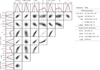 |
Fig. A.1. Resulting parameter distribution of WIII for the 2011 outburst of 4U 0115+63. Orbital distance is given in light-seconds, orbital velocity is given in units of speed-of-light, standard gravitational parameters are scaled for light-days and days, and the reference time is given in days. For |

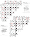 |
Fig. A.2. Resulting parameter distribution of WIII for the 2015 (top) and 2017 (bottom) outbursts of 4U 0115+63 (see Fig. A.1). |
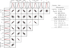 |
Fig. A.3. Resulting parameter distribution of WIII for the 2023 outburst of 4U 0115+63 (see Fig. A.1). |
All Tables
All Figures
|
Fig. 1. Sketch of the disk and magnetic field configuration for an accreting system (not to scale). The truncation radius Rt indicates where the matter, indicated by the mass accretion rate Ṁ, couples to the magnetic field. The co-rotation radius where the magnetic field lines rotate at the same speed as the local Keplerian speed is at Rco. The outer radius, Rout, indicates the outermost radius where the central magnetic field is connected to the disk. Beyond this radius the stress becomes too large, causing the field to disconnect from the central source. |
| In the text | |
|
Fig. 2. Torque function, n(ω), as a function of the model-dependent fastness, ω, for the torque models discussed in Sect. 3.2. The dashed lines correspond to models where Rt∝RA is assumed. The red crosses show the values obtained by Ireland et al. (2020); the black circles are from Ireland et al. (2022) (see Table 1 for an explanation of the labels). As discussed in the text, no conclusions concerning the relative behavior of n(ω) between the different models should be drawn from this figure. |
| In the text | |
|
Fig. 3. Relation between the model-dependent fastness, ωi, and the canonical fastness, |
| In the text | |
|
Fig. 4. Torque function of all considered models expressed via the canonical fastness. The labels indicate the models with the corresponding subscript. The dashed lines indicate models where Rt∝RA. The red crosses mark the results of Ireland et al. (2020) and the black circles that of Ireland et al. (2022). The black circles with a dot identify the simulations in the transition region of Fig. 3, with 0.6<ωi<0.8. |
| In the text | |
|
Fig. 5. Visual representation of the equilibrium fastness. The parameter is either ωp for Matt & Pudritz (2005) or ξ/γc for Dai & Li (2006). For ωp the lower bound is 1. All other models have fixed values for the equilibrium fastness (see Table 2) and are displayed over an arbitrary short range for clarity only. The dashed lines indicate models where Rt∝RA. |
| In the text | |
|
Fig. 6. Top panel: Predicted change in rotation period for all models (except Rappaport et al. 2004) for a given starting period and a mass accretion rate defined by a Poisson process. The colors indicate the models, as before. The dashed lines indicate models with Rt∝RA. Bottom panel: Simulated Poisson light curve. |
| In the text | |
|
Fig. 7. Torque modeling for 4U 0115+63. (a) Light curve of 4U 0115+63 as measured by Swift/BAT. The red curve is the interpolation of the data. (b) Pulsation period as measured by Fermi/GBM. The red curve is the best-fit model of WIII modified by the Doppler shift of the orbit. The green curve is the intrinsic spin-up of the NS. (c) Intrinsic spin-up signal predicted by the model (same as the green curve in panel (b). (d) χ residuals of the spin model. For all panels, the crosses enclosed by gray diamonds have been ignored for the model comparison; we also note the gaps on the time axis. |
| In the text | |
|
Fig. 8. Marginal probability distribution of the pole magnetic field strength estimated for all considered models. The colors indicate the identifier of the model. The dashed lines correspond to models with Rt∝RA. The gray area indicates the value range estimated from the CRSF features. |
| In the text | |
|
Fig. 9. Time dependence of the truncation radius for the unconstrained best fits for each model. The labels indicate the model corresponding to the predicted truncation radius. The dashed lines indicate models with Rt∝RA. The dotted black line marks the radius of co-rotation. |
| In the text | |
|
Fig. A.1. Resulting parameter distribution of WIII for the 2011 outburst of 4U 0115+63. Orbital distance is given in light-seconds, orbital velocity is given in units of speed-of-light, standard gravitational parameters are scaled for light-days and days, and the reference time is given in days. For |
| In the text | |
|
Fig. A.2. Resulting parameter distribution of WIII for the 2015 (top) and 2017 (bottom) outbursts of 4U 0115+63 (see Fig. A.1). |
| In the text | |
|
Fig. A.3. Resulting parameter distribution of WIII for the 2023 outburst of 4U 0115+63 (see Fig. A.1). |
| In the text | |
Current usage metrics show cumulative count of Article Views (full-text article views including HTML views, PDF and ePub downloads, according to the available data) and Abstracts Views on Vision4Press platform.
Data correspond to usage on the plateform after 2015. The current usage metrics is available 48-96 hours after online publication and is updated daily on week days.
Initial download of the metrics may take a while.