| Issue |
A&A
Volume 698, June 2025
|
|
|---|---|---|
| Article Number | A94 | |
| Number of page(s) | 9 | |
| Section | Cosmology (including clusters of galaxies) | |
| DOI | https://doi.org/10.1051/0004-6361/202453360 | |
| Published online | 03 June 2025 | |
Chemical enrichment of the intracluster medium within the A3266 cluster
I. Radial profiles
1
Max-Planck-Institut für extraterrestrische Physik, Gießenbachstraße 1, 85748 Garching, Germany
2
Institute for Frontiers in Astronomy and Astrophysics, Beijing Normal University, Beijing 102206, China
3
Institute of Astronomy, Madingley Road, Cambridge CB3 0HA, UK
4
INAF – IASF Palermo, Via U. La Malfa 153, I-90146 Palermo, Italy
5
School of Physics & Astronomy, University of Nottingham, University Park, Nottingham NG7 2RD, UK
6
Department of Astronomy, University of Geneva, Ch. d’Ecogia 16, CH-1290 Versoix, Switzerland
7
Department of Physics and Astronomy, University of Alabama in Huntsville, Huntsville, AL 35899, USA
8
Harvard-Smithsonian Center for Astrophysics, 60 Garden Street, Cambridge, MA 02138, USA
9
Department of Astrophysical Sciences, Princeton University, NJ 08544, USA
⋆ Corresponding author: This email address is being protected from spambots. You need JavaScript enabled to view it.
Received:
9
December
2024
Accepted:
17
April
2025
Abstract
We present a detailed study of the elemental abundances distribution of the intracluster medium (ICM) within the A3266 cluster using XMM-Newton observations. This analysis uses EPIC-pn data, including a new energy scale calibration, which allows us to measure velocities with uncertainties down to Δv ∼ 80 km/s, and MOS observations. We measured radial O, Mg, Si, S, Ar, Ca, and Fe profiles. This is the first study of elemental abundances beyond Fe using X-ray observations within the A3266 cluster. The abundance profiles display discontinuities similar to those obtained for the temperature. We modeled the X/Fe ratio profiles with a linear combination of type Ia supernovae (SNIa) and core-collapse supernovae (SNcc) models. We found that the SNIa ratio over the total cluster enrichment tends to be uniform, with a 42 ± 5% contribution. Such a trend supports an early ICM enrichment scenario, with most metals produced before clustering.
Key words: galaxies: clusters: intracluster medium / galaxies: clusters: individual: A3266 / X-rays: galaxies: clusters
© The Authors 2025
 Open Access article, published by EDP Sciences, under the terms of the Creative Commons Attribution License (https://creativecommons.org/licenses/by/4.0), which permits unrestricted use, distribution, and reproduction in any medium, provided the original work is properly cited.
This article is published in open access under the Subscribe to Open model.
Open Access funding provided by Max Planck Society.
1. Introduction
The intracluster medium (ICM) hosts most of the baryonic mass in a cluster of galaxies, thus providing crucial information on the origin and distribution of chemical elements during the evolution of the Universe. Fe-peak elements (Cr, Mn, Fe, Ni) mainly originate from type-Ia supernovae (SNIa), and light α-elements (O, Ne, Mg) are mainly produced in core-collapse supernovae (SNcc). Intermediate-mass elements (e.g., Si, S, Ar, and Ca) are synthesized by both SNIa and SNcc (e.g., Nomoto et al. 2013, and references therein). In this way, the ICM abundance distribution is sensitive to the number of SNIa and SNcc that contribute to chemical enrichment, the initial mass function (IMF) of the stars that explode as SNcc, the initial metallicity of the progenitors, the SNIa explosion mechanism, and the timescale over which the supernova products are expelled (see Werner et al. 2008, for a review). However, there is an intense debate regarding the SNIa explosion mechanisms, with the two main theoretical models proposed including pure deflagration (Plewa et al. 2004; Plewa 2007; Kasen & Plewa 2007; Fink et al. 2014; Long et al. 2014) and delayed denotation (Hoeflich & Khokhlov 1996; Iwamoto et al. 1999; Gamezo et al. 2005; Röpke et al. 2012). Therefore, accurate ICM abundance measurements will help to distinguish between both scenarios.
X-ray spectroscopy of the ICM provides a powerful tool to constrain the abundance distribution of these elements from their emission lines (Gatuzz et al. 2023a,b,c). A central Fe abundance excess has been found in many cool-core clusters (e.g., De Grandi & Molendi 2001; Churazov et al. 2003; Panagoulia et al. 2015; Mernier et al. 2017; Liu et al. 2019, 2020). Towards the outskirts, a flat and azimuthally uniform Fe distribution has been observed (Matsushita 2011; Werner et al. 2013; Simionescu et al. 2015; Urban et al. 2017). Furthermore, Hitomi observations of the Perseus cluster show abundance ratios entirely consistent with Solar abundance ratios (Hitomi Collaboration 2018; Simionescu et al. 2019). These results point out the importance of the contribution from both SNIa (with sub-Chandrasekhar mass) and near SNcc to the chemical enrichment of the ICM.
The A3266 galaxy cluster constitutes an excellent target to study the chemical enrichment of the ICM within a merging system. Henriksen & Tittley (2002) measured a nonmonotonically decreasing radial Fe profile using Chandra. A Fe abundance map was created by Sauvageot et al. (2005) with XMM-Newton data. They found that the Fe abundance map indicates that metals are inhomogeneously distributed across the cluster due to the merging features of the system. However, they did not measure individual elemental abundances. A3266 was a calibration target of the eROSITA X-ray telescope (Predehl et al. 2021) on board the Spectrum Roentgen Gamma (SRG) observatory. In their data analysis, Sanders et al. (2022) identified three different subclusters merging with the main body of the cluster. These systems appear associated with higher-metallicity gas.
Gatuzz et al. (2024) studied the velocity structure within the A3266 galaxy cluster using XMM-Newton observations. They observed that the hot gas moves with a redshifted systemic velocity relative to the cluster core across all fields of view. Here, we present a detailed study of the elemental abundance distribution within the A3266 galaxy cluster. The outline of this paper is as follows. We describe the data reduction process in Sect. 2. In Sect. 3 we explain the fitting procedure. A discussion of the results is shown in Sect. 4. Finally, Sect. 5 includes the conclusions and summary. Throughout this paper we assume the distance of A3266 to be z = 0.0594 (Dehghan et al. 2017) and a concordance ΛCDM cosmology with Ωm = 0.3, ΩΛ = 0.7, and H0 = 70 km s−1 Mpc−1.
2. Data reduction
We used the same observations analyzed in Gatuzz et al. (2024) and followed the reduction process shown in Sanders et al. (2020) and Gatuzz et al. (2022). The XMM-Newton European Photon Imaging Camera (EPIC, Strüder et al. 2001) spectra were reduced with the Science Analysis System (SAS1, version 21.0.0). We decided to include spectra from both the Metal Oxide Semi-conductor (MOS) and pn instruments in our analysis, operating in full frame mode and extended full frame mode, respectively. We reduce the pn, MOS 1, and MOS 2 data using the SAS epchain and emchain tools. We filtered the data using FLAG= = 0 to avoid bad pixels or regions close to the charge-coupled device (CCD) edges. We used the single, double, triple, and quadruple events in MOS (PATTERN ≤ 12), while we used only single-pixel events for the pn instrument (PATTERN= = 0). We also identified and discarded those EPIC MOS chips in the anomalous state using the emanom task. We created the EPIC-pn event files, including the new energy calibration scale developed in Sanders et al. (2020) and Gatuzz et al. (2022), to obtain velocity measurements down to 150 km/s at Fe-K by using the instrumental X-ray background lines as references for the absolute energy scale. Point-like sources were identified and removed from the subsequent analysis by using the SAS edetect_chain tool, with a likelihood parameter det_ml > 10
For the pn camera, we filtered bad time intervals from flares with a 1.0 cts/s rate threshold to be consistent with the Gatuzz et al. (2024) procedure. We built the Good Time Intervals for the MOS cameras by applying the 2σ clipping technique (Mernier et al. 2015), which we now explain in detail. First, we extract the count-rate histogram from the light curves in the 10 − 12 keV energy range. After binning them in 100 s intervals, we fit them with a Gaussian function, and we reject all time bins for which the number of counts lies outside the interval μ ± 2σ, where μ is the fitted average of the distribution. Then, we repeat the same procedure for 10 s binned histograms in the 0.3 − 10 keV energy range to remove soft background flares. We iterate through this process and manually inspect the light curves until all flares are removed. To study the distribution of chemical elements in the ICM, we analyze non-overlapping rings whose radii increase as the square root with distance from the A3266 center. Figure 1 shows the exposure-vignetting-corrected and a background-subtracted X-ray image of the A3266 cluster in the 0.5–9.25 keV energy range obtained for the EPIC-pn instrument. The figure also included the annular rings that correspond to the spectra extraction regions. The radius of the annular regions increases up to ∼1125 kpc. The obtained spectra have more than 5 × 10⁵ counts in the analyzed energy range.
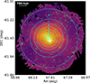 |
Fig. 1. Exposure-vignetting-corrected and background-subtracted X-ray image of the A3266 cluster in the 0.5–9.25 keV energy range obtained for the EPIC-pn instrument. Cyan rings correspond to the analyzed Regions, while green circles correspond to point sources that were excluded from the analysis. |
We extracted the EPIC-pn spectra following the procedure described by Sanders et al. (2020). The spectra were extracted using the evselect task, covering channels 0-20479. The response matrix was generated with the rmfgen task, which employed a fine energy grid with a resolution of 0.3 eV. Auxiliary response files (ARFs) were created using the arfgen task, with the setbackscale and extendedsource parameters set to yes. The MOS spectra were extracted using the evselect task, covering channels 0-11999. The response files were also extracted using the rmfgen task, spanning the 0.1–12 keV energy range with a total of 1190 energy bins. The ARFs were generated using the arfgen task, with the parameter extendedsource set to yes. For the EPIC spectra, we applied binning using the standard factor of five PI channels (i.e., 5 eV bins).
3. Spectral fitting
We combine the spectra from different observations for each spatial Region shown in Fig. 1. The new EPIC-pn energy calibration scale cannot be applied to lower energies; therefore, we load the data twice to fit separately, but simultaneously, the soft (0.5 − 4.0 keV) and hard (4.0 − 10 keV) energy bands. The previous work in Gatuzz et al. (2024) only included the hard band. The MOS spectra are fit in the 0.5 − 10 keV energy range. We fit the spectra with the xspec spectral fitting package (version 12.14.12). Abundances are given relative to Lodders et al. (2009). We rebin the data to have at least one count per channel and we assumed cash statistics (Cash 1979). Errors are quoted at a 1σ confidence level unless otherwise stated.
We assume that the ICM is in collisional ionization equilibrium (CIE), and we use a single vapec thermal model to fit the spectra. vapec is a variant of the widely used apec model, including variable abundances for most abundant elements. The free parameters include the temperature (Te), elemental abundances (O, Mg, Si, Ar, S, Ca, Fe), redshift, and normalization. To account for the Galactic absorption, we included a tbabs component (Wilms et al. 2000), and fixed the column density to 2.26 × 1020 cm−2 (HI4PI Collaboration 2016). As discussed in Gatuzz et al. (2023a,b,c), we set the Al and Ni abundances to the Fe abundance, as their measurements may not be reliable due to instrumental background lines. We also link the Ne abundance to Fe, as the Fe L lines are located in the same spectral Region, which could possibly lead to confusion between the lines. Other abundances with Z ≥ 6 are also fixed to the Fe value.
Fitting the EPIC spectra over an extensive energy range can lead to slight under- or overestimation of the continuum emission in specific bands due to imperfections in the EPIC instrument calibration (see Mernier et al. 2015, 2016a). These discrepancies can, in turn, affect the derived elemental abundances, as the equivalent width (EW) of emission lines depends on the ratio between the line and the continuum flux. To correct these effects, we employed a local-fit method that refines the derived abundances by fitting narrower energy ranges centered around the strongest emission lines of each element. Mernier et al. (2015) found that systematics in individual abundance measurements are reduced to < 15% when applying this local fit method, thus more accurately determining line-to-continuum ratios. In this approach, we first performed a global spectra fit using the energy range of 0.5 − 10 keV for both EPIC-pn and MOS. We re-fitted the spectra within local energy bands to refine the abundance measurements. We chose to focus on the strongest K-shell emission lines of each element (except Ne, whose strongest lines are unresolved in the EPIC spectra). The energy ranges for the local fits are 0.50 − 0.80 keV (for O), 1.20 − 1.65 keV (for Mg), 1.65 − 2.26 keV (for Si), 2.27 − 3 keV (for S and Ar), 3.5 − 4.5 keV (for Ca), and 6.25 − 10. keV (for Fe). During these local fits, the global best-fit temperature was fixed to preserve the global thermal structure of the plasma. In contrast, the local normalization (emission measure) and the abundance of the element of interest were left free. This conservative approach accounts for systematic uncertainties related to EPIC cross-calibration issues and ensures robust abundance measurements. Additionally, we verified that the local-fit abundances were consistent within 2σ with the global-fit results for most elements, which confirms that the local corrections did not introduce significant biases. All abundance measurements presented in this work are corrected hereafter using the local-fit method.
The background model consists of two main components: the instrumental background and the astrophysical background. The astrophysical background consists of the unresolved population of point sources, modeled by a power law with Γ = 1.45 (Sanders et al. 2020), the local hot bubble (LHB) emission, modeled by one unabsorbed thermal plasma model (apec), and the Galactic halo emission (GH, e.g., Yoshino et al. 2009), which consist of one absorbed thermal plasma model (apec). For the thermal models, we use the temperatures obtained for A3266 by Sanders et al. (2022) in their analysis with the SRG/eROSITA X-ray telescope (Predehl et al. 2021) on board the SRG observatory. In particular, we fixed the temperatures to 0.133 keV for the LHB and 0.241 kev for the GH. The abundance of both components was kept proto-solar.
The instrumental background consists of a broken power-law (not folded by the effective area) to model the hard particle background (Mernier et al. 2015), a power law (not folded by the effective area) to model the soft-proton background (Erdim et al. 2021), and several instrumental profiles. This approach follows the methodology that we applied in our previous analysis of the Virgo (Gatuzz et al. 2023a), Centaurus (Gatuzz et al. 2023d), and Ophiuchus (Gatuzz et al. 2023c) galaxy clusters. For the EPIC-pn spectra, we included the Al Kα (1.49 keV), Ni Kα (7.84 keV), Cu Kα (8.04 keV), Zn Kα (8.64 keV), and Cu Kβ (8.90 keV) instrumental background lines. We included the Al Kα (1.49 keV) and Si Kα (1.75 keV) lines for the MOS spectra. The redshifts of the background lines were tied together and allowed to vary. The normalizations of the lines were free to vary. We fixed the soft-proton background for the EPIC-pn instrument to Γ = 0.136 to be consistent with Sanders et al. (2020). Following Erdim et al. (2021), we fixed the breaking point of the broken power-law at 3.0 keV. The lower limit of the photon index (Γ1) was left free to vary within 0.1–1.4, and the upper limit of the photon index (Γ2) was allowed to reach up to 2.5. We initially obtained best-fitting values for the hard particle and soft-proton background for the entire field of view (i.e., a circular Region with a radius equal to the outer border of ring eight shown in Fig. 1). Then, we only kept the normalization as a free parameter in the fits of the individual rings. The normalizations of the different background model components vary across the Regions analyzed during the global fit. During the local fits, which we performed to estimate the abundances better, the background model normalizations are fixed to the value obtained in the global fit.
Figure 2 shows an example spectrum and residuals from this analysis (i.e., for Region 2). The solid line indicates the best-fitting apec model. Vertical dashed lines indicate the instrumental Al Kα, Si Kα, Ni Kα, Cu Kα,β, and Zn Kα background lines included in the model. Vertical solid lines indicate the contribution of O, Mg, Si, S, Ar, Ca, and Fe to the line emission. Table 1 shows the best-fit parameters obtained for each ring. We noted that the background component increases as we move towards the cluster outskirts. Previous studies have found such variation and reflect the spectral decomposition and degeneracy with cluster emission (Urban et al. 2011; Walker et al. 2019). In the inner Regions where the cluster emission is bright, the contribution of the soft X-ray background component LHB and GB is relatively minor. In contrast, where the cluster surface brightness decreases at larger radii, the relative contribution of the LHB and GB components becomes more prominent, and their normalizations are better constrained. Furthermore, the GH emission exhibits some degree of spatial variation on large scales due to differences in Galactic column density and the presence of local structures in the hot gas distribution (Yoshino et al. 2009; Henley & Shelton 2013). To test the significance of this variation, we performed fits with fixed LHB and GH normalizations (determined from the complete Region) and found that while the overall fit statistic worsened slightly, the cluster parameters remained consistent within uncertainties. This suggests that while there is an apparent increase in the background normalizations, the effect does not strongly bias our primary cluster measurements. We also tested additional models for the ICM component, including a two apec thermal components model and a lognorm model (Gatuzz et al. 2023b). Figure 3 compares the best-fitting statistic obtained for each model. The numbering is from the innermost to the outermost. However, the best-fit cash statistic (C-stat) value remained very similar for the different models. Therefore, we decided to analyze the A3266 cluster using the single-temperature model.
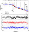 |
Fig. 2. Example spectrum and best-fit model obtained from the global fit for Region 2. The spectrum has been rebinned for illustrative purposes. EPIC-pn (black points), MOS1 (red points), and MOS2 (blue points) have been included. The line contribution from instrumental background (vertical dashed lines) and ICM emission (vertical solid lines) are indicated. The lower panel shows the residuals of the fit for each instrument. |
A3266 cluster best-fit parameters for annular Regions.
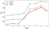 |
Fig. 3. Best-fitting Cash statistic obtained with the 1-apec, 2-apec, and lognorm models. |
To assess the impact of background modeling uncertainties on our measured abundances, we performed a test in which we varied the normalizations of the instrumental and astrophysical background components by ±30%. We found that increasing the background by 30% resulted in a significantly worse fit (e.g., the C-stat increased from cstat = 6933 to cstat = 13 695 in the innermost Region). Such a large degradation in fit quality suggests that a 30% increase is not a physically reasonable scenario for our data. Given that our best-fit background models have uncertainties of less than 10%, we performed a more realistic test by varying the background components within ±10%. In this case, the measured abundances remained consistent within statistical uncertainties, which indicates that our abundance measurements are robust against reasonable variations in background modeling. This test also suggests that the abundances of elements with weak emission lines, such as O, Si, S, Ar, and Ca, are not significantly biased by continuum fitting effects. The consistency of the abundance measurements under realistic background variations reinforces the reliability of our spectral fitting approach.
4. Results and discussion
In this section we discuss the best-fit results obtained.
4.1. Temperature profile
Figure 4 shows the temperature values obtained from the best fit per Region. The temperatures are generally similar to those obtained by Gatuzz et al. (2024), except for Regions 1 and 8, where temperatures obtained are larger and lower, respectively. We identified evident discontinuities at ∼350 kpc and ∼800 kpc, which can also be observed in the surface brightness map computed by Gatuzz et al. (2024). The temperature in the 600 − 800 kpc range is constant. Such discontinuities could be associated with subgroups within the system, as identified by Dehghan et al. (2017).
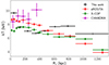 |
Fig. 4. Top panel: Temperature profile obtained from the global fit. The figure also includes the temperature profiles obtained with eROSITA (Sanders et al. 2022), X-COP (Ghirardini et al. 2019), and Chandra (Henriksen & Tittley 2002). |
Figure 4 also includes the temperature profiles obtained with eROSITA (Sanders et al. 2022, red points), XMM-Newton Cluster Outskirts Project (X-COP, Ghirardini et al. 2019, green points), and Chandra (Henriksen & Tittley 2002, magenta points). Sauvageot et al. (2005) also found high temperatures (kT > 12) for the inner Region. Temperatures are also similar to those obtained by Sanders et al. (2022). The high temperature near the cluster core could be due to active galactic nuclei (AGN) activity. A similar trend of temperature increasing and then decreasing for distances > 800 kpc was found in the Chandra data (Henriksen & Tittley 2002).
The discrepancy between the temperatures obtained for large distances from different telescopes may be due to several factors, including calibration differences, as discussed in Sanders et al. (2022). The differences between our measured temperature profile for A3266 and the results presented in the X-COP study can be attributed to several factors. First, our study benefits from approximately eight times the exposure time used in X-COP. Furthermore, we use NH = 2.26 × 1020 cm−2, while X-COP adopts NH = 1.62 × 1020 cm−2, leading to systematic differences in the derived temperatures, particularly at lower energies where absorption is more significant. Additionally, our analysis includes all spectra in the 0.5 − 10 keV energy range, whereas X-COP excludes specific energy bands (1.2 − 1.9 keV for MOS, 1.2 − 1.7 keV and 7.0 − 9.2 keV for pn) to mitigate instrumental background effects. The exclusion of these bands in X-COP likely impacts the temperature measurements, especially in Regions dominated by background. Differences in atomic data also contribute, as we employ the latest APEC version with updated atomic data, while X-COP used an earlier version. Background modeling differences and the treatment of element abundances also play a role; our analysis allows individual element abundances to vary as free parameters, unlike X-COP, which scales all abundances to Fe. This distinction affects the coupling between temperature and metallicity in spectral fitting and can impact the resulting temperature profile. Notably, when we fix NH to the X-COP value and adopt a simplified abundance model with all abundances equal to Fe, the temperature profile at large radii decreases and aligns more closely with the X-COP results. These considerations explain the observed discrepancies with X-COP results.
4.2. Velocity profile
The velocities obtained for each Region are shown in Fig. 5. As in our previous series of analyses of the ICM in galaxy clusters, these velocities correspond to the redshift obtained with the vapec model with respect to the source redshift (z = 0.0594). This redshift corresponds to the mean redshift of the cluster core and was obtained from spectroscopic redshifts of 1300 sources within the cluster by Dehghan et al. (2017). We have obtained velocities with uncertainties down to Δv ∼ 80 km/s (Region 8). The largest blueshift and redshift obtained, with respect to the A3266 systemic redshift, correspond to 635 ± 276 km/s (Region 1) and −313 ± 102 km/s (Region 7). Figure 5 also includes the velocities obtained by Gatuzz et al. (2024), which agree with the current results, even though we have included the soft-energy band. Moreover, including the MOS data leads to a better constraint on the velocity measurement. The significant discrepancy in the outermost Region compared to Gatuzz et al. (2024) likely arises from a combination of factors: (1) higher astrophysical background in the cluster outskirts (see Table 1), which may affect the accuracy of Fe Kα centroid measurements, especially in low signal-to-background Regions; (2) projection effects and dynamical complexity in the cluster outskirts; and (3) the inclusion of EPIC-MOS spectra, which reduces velocity uncertainties overall but may amplify sensitivity to background modeling in Regions with low signal. Notably, the velocities agree elsewhere, which suggests that the discrepancy in the outermost Region is driven by the challenging observational conditions there.
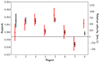 |
Fig. 5. Comparison between the velocities obtained for each Region (black points) and those obtained by Gatuzz et al. (2024, red points). The horizontal line indicates the A3266 cluster redshift (z = 0.0594). |
4.3. Abundance profiles
The best-fit elemental abundances obtained per Region with respect to the Solar values are shown in Fig. 7. For comparison, Fig. 6 shows all elements in a combined plot. This is the first study of elemental abundances using X-ray observations within the A3266 cluster. The abundance uncertainties are somewhat large, most likely because the emission lines show low strength due to the high temperature, and therefore high ionization state, of the ICM (for comparison with low-temperature systems such as Virgo and Centaurus see Gatuzz et al. 2023a,b). O, Mg, and Si derived abundances display positive gradients for distances < 600 kpc before they become flatter. The Ca abundance displays a flat profile for lower distances. All elements show a similar abundance in the 600 − 800 kpc range, similar to the trend observed in the temperature.
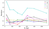 |
Fig. 6. A3266 radial abundances distribution for each element. Uncertainties are not included for illustrative purposes. |
 |
Fig. 7. A3266 abundance profiles obtained from the local fits. |
In general, the abundance profiles display similar discontinuities to those obtained for the temperature (see Fig. 4) Interestingly, the Fe profile does not display a large dispersion, a trend also identified in Chandra observations (Henriksen & Tittley 2002). The high metallicity at large distances may indicate the mixing of metal-rich gas in the outskirts, most likely due to complex merger activities (Sun et al. 2002; Urdampilleta et al. 2019; Walker & Lau 2022). A similar trend was identified in Ophiuchus, another system with merging features (Gatuzz et al. 2023c). We have also not found any drop in the metallicity for the inner Region of the cluster (see, for example, the Centaurus analysis in Gatuzz et al. 2023b). However, the spatial scale of the innermost Region analyzed is much larger than the physical radius for which a drop in Fe abundance has been identified in other sources. Finally, we have not found a correlation between the abundance and the velocity profiles. In order to better understand the dynamics and kinematics within such a system, future comparisons with detailed hydrodynamical simulations, including cluster merging events, are crucial.
Abundance determination using EPIC-pn implies limitations and caveats. Despite the effort to improve the calibration (de Plaa et al. 2007; Read et al. 2014; Schellenberger et al. 2015), cross-calibration differences between EPIC instruments have been reported. Low-temperature systems (i.e., kT ∼ 0.7 keV) tend to display a strong degeneracy between the emission measure and the metallicities (Mernier et al. 2022). The so-called Fe bias occurs when a single-temperature plasma model is used for a multitemperature ICM condition (Buote & Fabian 1998; Mernier et al. 2018; Gastaldello et al. 2021). However, we found that the best-fit abundances obtained with the vapec model agree with those obtained with the vlognorm model within 1σ, although uncertainties tend to be lower for the multitemperature model. Other limitations may arise from systematic uncertainties associated with the astrophysical or instrumental background. In that sense, the global-local fit procedure followed in this work, and simultaneously fitting pn and MOS instruments, is considered the most robust one (Mernier et al. 2015; Fukushima et al. 2022).
4.4. ICM chemical enrichment from SN
We computed X/Fe ratio profiles for O, Mg, Si, Ar, S, and Ca (gray shaded Regions in Fig. 8). Considering the uncertainties, we found that O/Fe, Mg/Fe, S/Fe, and Ca/Fe abundance ratios are close to the proto-solar values for all distances. On the other hand, the Si/Fe tends to be lower, and the Ar/Fe is higher (> 2 Solar) for all distances. Mernier et al. (2015) indicated that Ar abundances most likely suffer from instrumental systematics when comparing EPIC-pn with MOS spectra.
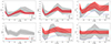 |
Fig. 8. Abundance ratio profiles, relative to Fe, obtained from the local fits. The gray shaded areas indicate the mean values and the 1σ errors. The SNcc (blue line) and SNIa (green line) contribution to the total SN ratio (red shaded area) from the best-fit model are included (see Sect. 4.4). |
We used the abundfit.py python code developed by Mernier et al. (2016b) to model the contribution from different supernova (SN) yield models to the abundance ratio profiles obtained. The code fits a combination of multiple progenitor yield models to compute the relative contribution that fits better a given set of ICM abundances. For the SNcc and SNIa yields, we have included multiple models listed in Table 2. The SNcc yields were integrated with Salpeter IMF, while for SNIa, we considered models that included a variety of explosion mechanisms. Such models have been used in previous enrichment studies (Mernier et al. 2017; Simionescu et al. 2019; Mernier et al. 2020; Gatuzz et al. 2023a,b,c). However, it is worth mentioning that further effortto improve theoretical models of supernova nucleosynthesis is essential to reduce uncertainties in the yield calculations (e.g., including neutrino physics).
SNIa and SNcc yields included in the modeling of the X/Fe profiles.
We used the same model along the radii to represent the profile, allowing us to determine the SN ratio profile at all measured distances. Then, we determined the best linear combination of SNIa and SNcc models that better fit the abundance ratio profiles by minimizing the sum of their χ2 values in quadrature. The best-fit model (χ2/d.o.f. = 50.1/48 = 1.04) corresponds to Nomoto et al. (2006) with an initial metallicity of Z = 0.01 for the SNcc and the dynamically driven double-degenerate double-detonation by Shen et al. (2018) with the parameters M10, 3070, Z = 0.01 for the SNIa contribution. Figure 8 shows the SNIa contribution (green line) and the SNcc contribution (blue line) to the total SNe ratio (red shaded Region). We found that the SNcc contribution is more significant than the SNIa contribution for almost all radii. The contribution from SNIa to the total enrichment by this set of models is shown in Fig. 9. A linear fit gives almost zero slope (2.69 × 10⁻⁵ with χ2 = 1.14) and a constant value of 0.42 ± 0.05, which verifies that the SNIa contribution to the total SNe tends to be constant. Such a consistent radial profile may suggest that the SNIcc and SNIa components occurred at similar epochs.
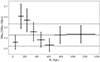 |
Fig. 9. SNIa contribution to the total chemical enrichment as a function of the distance. The model includes O, Mg, Si, S, Ar, Ca, and Fe abundances. The black line represents the 1σ confidence interval of constant fit. |
These results support an early ICM enrichment scenario, with most of the metals present being produced prior to clustering, in agreement with our previous results for Virgo (Werner et al. 2006; Simionescu et al. 2010; Million et al. 2011; Gatuzz et al. 2023a), Centaurus (Sanders et al. 2016; Mernier et al. 2017; Gatuzz et al. 2023b), and Ophiuchus (Gatuzz et al. 2023c). Compared with those previous works, our abundance ratio shows less scattering, most likely due to the inclusion of MOS spectra in the spectral fit. As seen in Fig. 8, the SNe model reproduces the observed pattern abundance for almost all elements except for Ar. It is essential to mention that different contributions of the same SNIa and SNcc models also lead to good fits when compared with the measured abundance ratios (i.e., χ2 < 1.2). Therefore, such models can only be partially dismissed.
The observed enrichment pattern indicates that the merging progenitors had comparable chemical histories, with most ICM metals produced before the cluster assembly. Furthermore, the absence of distinct metal-rich cores breaking apart during the merger implies significant mixing of the ICM, likely driven by merger-induced turbulence and shocks. Such behavior contrasts with nonmerging clusters, where more pronounced metallicity gradients are often observed. These findings emphasize the role of mergers in shaping the chemical properties of the ICM and highlight the need for simulations that incorporate merger dynamics better to understand the interplay between cluster evolution and chemical enrichment.
5. Conclusions and summary
We have analyzed XMM-Newton EPIC observations of the A3266 galaxy cluster to study the radial profiles of physical parameters such as temperature and the O, Mg, Si, S, Ar, Ca, and Fe distribution in the ICM. This is the first analysis of such profiles for A3266. This work expands upon the outcomes of Gatuzz et al. (2024) by including the soft energy band < 4 keV and MOS spectra. Our main findings and conclusions are:
-
We modeled the ICM emission using a single temperature model. From a statistical point of view, there is no improvement in the fit when including a more complex model, most likely because of the high temperature of the system.
-
We found velocities in good agreement with Gatuzz et al. (2024). Moreover, including MOS spectra leads to lower uncertainties, Δv ∼ 80 km/s. There is no clear trend between the velocities and other physical parameters such as temperature or abundance.
-
The temperature shows discontinuities at ∼350 kpc and ∼800 kpc. This could be associated with the presence of subgroups.
-
We obtained abundance profiles for O, Mg, Si, S, Ar, Ca, and Fe. Most of the elements display the same discontinuities found for the temperature.
-
We modeled X/Fe abundance ratio profiles with a linear combination of SNcc and SNIa. We found that the best-fit model corresponds to a dynamically driven double-degenerate double-detonation for the SNcc contribution and an SNcc model with an initial metallicity of Z = 0.01. This model reproduces the abundance ratios, except for Ar.
-
We found that the SNIa ratio over the total cluster enrichment tends to be uniform. Such uniformity in the SNIa percentage contribution supports an early enrichment of the ICM scenario, where most of the metals present were produced before clustering.
Acknowledgments
This work was supported by the Deutsche Zentrum für Luft- und Raumfahrt (DLR) under the Verbundforschung programme (Messung von Schwapp-, Verschmelzungs- und Rückkopplungsgeschwindigkeiten in Galaxienhaufen.). This work is based on observations obtained with XMM-Newton, an ESA science mission with instruments and contributions directly funded by ESA Member States and NASA. This research was carried out on the High-Performance Computing resources of the Raven and Viper clusters at the Max Planck Computing and Data Facility (MPCDF) in Garching, operated by the Max Planck Society (MPG).
References
- Badenes, C., Borkowski, K. J., Hughes, J. P., Hwang, U., & Bravo, E. 2006, ApJ, 645, 1373 [NASA ADS] [CrossRef] [Google Scholar]
- Buote, D. A., & Fabian, A. C. 1998, MNRAS, 296, 977 [NASA ADS] [CrossRef] [Google Scholar]
- Cash, W. 1979, ApJ, 228, 939 [Google Scholar]
- Chieffi, A., & Limongi, M. 2004, ApJ, 608, 405 [NASA ADS] [CrossRef] [Google Scholar]
- Churazov, E., Forman, W., Jones, C., & Böhringer, H. 2003, ApJ, 590, 225 [NASA ADS] [CrossRef] [Google Scholar]
- De Grandi, S., & Molendi, S. 2001, ApJ, 551, 153 [NASA ADS] [CrossRef] [Google Scholar]
- de Plaa, J., Werner, N., Bleeker, J. A. M., et al. 2007, A&A, 465, 345 [NASA ADS] [CrossRef] [EDP Sciences] [Google Scholar]
- Dehghan, S., Johnston-Hollitt, M., Colless, M., & Miller, R. 2017, MNRAS, 468, 2645 [NASA ADS] [CrossRef] [Google Scholar]
- Erdim, M. K., Ezer, C., Ünver, O., Hazar, F., & Hudaverdi, M. 2021, MNRAS, 508, 3337 [Google Scholar]
- Fink, M., Kromer, M., Seitenzahl, I. R., et al. 2014, MNRAS, 438, 1762 [NASA ADS] [CrossRef] [Google Scholar]
- Fukushima, K., Kobayashi, S. B., & Matsushita, K. 2022, MNRAS, 514, 4222 [NASA ADS] [CrossRef] [Google Scholar]
- Gamezo, V. N., Khokhlov, A. M., & Oran, E. S. 2005, ApJ, 623, 337 [NASA ADS] [CrossRef] [Google Scholar]
- Gastaldello, F., Simionescu, A., Mernier, F., et al. 2021, Universe, 7, 208 [NASA ADS] [CrossRef] [Google Scholar]
- Gatuzz, E., Sanders, J. S., Dennerl, K., et al. 2022, MNRAS, 511, 4511 [NASA ADS] [CrossRef] [Google Scholar]
- Gatuzz, E., Sanders, J. S., Dennerl, K., et al. 2023a, MNRAS, 520, 4793 [NASA ADS] [CrossRef] [Google Scholar]
- Gatuzz, E., Sanders, J. S., Dennerl, K., et al. 2023b, MNRAS, 525, 6394 [NASA ADS] [CrossRef] [Google Scholar]
- Gatuzz, E., Sanders, J. S., Dennerl, K., et al. 2023c, MNRAS, 526, 396 [NASA ADS] [CrossRef] [Google Scholar]
- Gatuzz, E., Mohapatra, R., Federrath, C., et al. 2023d, MNRAS, 524, 2945 [NASA ADS] [CrossRef] [Google Scholar]
- Gatuzz, E., Sanders, J., Liu, A., et al. 2024, A&A, 692, A108 [NASA ADS] [CrossRef] [EDP Sciences] [Google Scholar]
- Ghirardini, V., Eckert, D., Ettori, S., et al. 2019, A&A, 621, A41 [NASA ADS] [CrossRef] [EDP Sciences] [Google Scholar]
- Heger, A., & Woosley, S. E. 2010, ApJ, 724, 341 [Google Scholar]
- Henley, D. B., & Shelton, R. L. 2013, ApJ, 773, 92 [NASA ADS] [CrossRef] [Google Scholar]
- Henriksen, M. J., & Tittley, E. R. 2002, ApJ, 577, 701 [NASA ADS] [CrossRef] [Google Scholar]
- HI4PI Collaboration (Ben Bekhti, N., et al.) 2016, A&A, 594, A116 [NASA ADS] [CrossRef] [EDP Sciences] [Google Scholar]
- Hitomi Collaboration (Aharonian, F., et al.) 2018, PASJ, 70, 12 [NASA ADS] [Google Scholar]
- Hoeflich, P., & Khokhlov, A. 1996, ApJ, 457, 500 [CrossRef] [Google Scholar]
- Iwamoto, K., Brachwitz, F., Nomoto, K., et al. 1999, ApJS, 125, 439 [NASA ADS] [CrossRef] [Google Scholar]
- Kasen, D., & Plewa, T. 2007, ApJ, 662, 459 [NASA ADS] [CrossRef] [Google Scholar]
- Kromer, M., Pakmor, R., Taubenberger, S., et al. 2013, ApJ, 778, L18 [NASA ADS] [CrossRef] [Google Scholar]
- Kromer, M., Ohlmann, S. T., Pakmor, R., et al. 2015, MNRAS, 450, 3045 [NASA ADS] [CrossRef] [Google Scholar]
- Leung, S.-C., & Nomoto, K. 2018, ApJ, 861, 143 [Google Scholar]
- Liu, A., Zhai, M., & Tozzi, P. 2019, MNRAS, 485, 1651 [NASA ADS] [CrossRef] [Google Scholar]
- Liu, A., Tozzi, P., Ettori, S., et al. 2020, A&A, 637, A58 [NASA ADS] [CrossRef] [EDP Sciences] [Google Scholar]
- Lodders, K., Palme, H., & Gail, H. P. 2009, Solar System, Landolt-Börnstein, Group VI Astronomy and Astrophysics, 4B (Berlin, Heidelberg: Springer-Verlag), 712 [Google Scholar]
- Long, M., Jordan, G. C. I., van Rossum, D. R., et al. 2014, ApJ, 789, 103 [NASA ADS] [CrossRef] [Google Scholar]
- Maeda, K., Röpke, F. K., Fink, M., et al. 2010, ApJ, 712, 624 [CrossRef] [Google Scholar]
- Marquardt, K. S., Sim, S. A., Ruiter, A. J., et al. 2015, A&A, 580, A118 [NASA ADS] [CrossRef] [EDP Sciences] [Google Scholar]
- Matsushita, K. 2011, A&A, 527, A134 [EDP Sciences] [Google Scholar]
- Mernier, F., & Biffi, V. 2022, in Handbook of X-ray and Gamma-ray Astrophysics, eds. C. Bambi, & A. Santangelo, 12 [Google Scholar]
- Mernier, F., de Plaa, J., Lovisari, L., et al. 2015, A&A, 575, A37 [NASA ADS] [CrossRef] [EDP Sciences] [Google Scholar]
- Mernier, F., de Plaa, J., Pinto, C., et al. 2016a, A&A, 592, A157 [NASA ADS] [CrossRef] [EDP Sciences] [Google Scholar]
- Mernier, F., de Plaa, J., Pinto, C., et al. 2016b, A&A, 595, A126 [NASA ADS] [CrossRef] [EDP Sciences] [Google Scholar]
- Mernier, F., de Plaa, J., Kaastra, J. S., et al. 2017, A&A, 603, A80 [NASA ADS] [CrossRef] [EDP Sciences] [Google Scholar]
- Mernier, F., Biffi, V., Yamaguchi, H., et al. 2018, Space Sci. Rev., 214, 129 [Google Scholar]
- Mernier, F., Cucchetti, E., Tornatore, L., et al. 2020, A&A, 642, A90 [NASA ADS] [CrossRef] [EDP Sciences] [Google Scholar]
- Million, E. T., Werner, N., Simionescu, A., & Allen, S. W. 2011, MNRAS, 418, 2744 [NASA ADS] [CrossRef] [Google Scholar]
- Nomoto, K., Tominaga, N., Umeda, H., Kobayashi, C., & Maeda, K. 2006, Nucl. Phys. A, 777, 424 [CrossRef] [Google Scholar]
- Nomoto, K., Kobayashi, C., & Tominaga, N. 2013, ARA&A, 51, 457 [CrossRef] [Google Scholar]
- Ohlmann, S. T., Kromer, M., Fink, M., et al. 2014, A&A, 572, A57 [NASA ADS] [CrossRef] [EDP Sciences] [Google Scholar]
- Pakmor, R., Kromer, M., Röpke, F. K., et al. 2010, Nature, 463, 61 [Google Scholar]
- Pakmor, R., Edelmann, P., Röpke, F. K., & Hillebrandt, W. 2012, MNRAS, 424, 2222 [Google Scholar]
- Panagoulia, E. K., Sanders, J. S., & Fabian, A. C. 2015, MNRAS, 447, 417 [CrossRef] [Google Scholar]
- Plewa, T. 2007, ApJ, 657, 942 [NASA ADS] [CrossRef] [Google Scholar]
- Plewa, T., Calder, A. C., & Lamb, D. Q. 2004, ApJ, 612, L37 [Google Scholar]
- Predehl, P., Andritschke, R., Arefiev, V., et al. 2021, A&A, 647, A1 [EDP Sciences] [Google Scholar]
- Read, A. M., Guainazzi, M., & Sembay, S. 2014, A&A, 564, A75 [NASA ADS] [CrossRef] [EDP Sciences] [Google Scholar]
- Romano, D., Karakas, A. I., Tosi, M., & Matteucci, F. 2010, A&A, 522, A32 [NASA ADS] [CrossRef] [EDP Sciences] [Google Scholar]
- Röpke, F. K., Kromer, M., Seitenzahl, I. R., et al. 2012, ApJ, 750, L19 [CrossRef] [Google Scholar]
- Sanders, J. S., Fabian, A. C., Taylor, G. B., et al. 2016, MNRAS, 457, 82 [Google Scholar]
- Sanders, J. S., Dennerl, K., Russell, H. R., et al. 2020, A&A, 633, A42 [EDP Sciences] [Google Scholar]
- Sanders, J. S., Biffi, V., Brüggen, M., et al. 2022, A&A, 661, A36 [NASA ADS] [CrossRef] [EDP Sciences] [Google Scholar]
- Sauvageot, J. L., Belsole, E., & Pratt, G. W. 2005, A&A, 444, 673 [NASA ADS] [CrossRef] [EDP Sciences] [Google Scholar]
- Schellenberger, G., Reiprich, T. H., Lovisari, L., Nevalainen, J., & David, L. 2015, A&A, 575, A30 [NASA ADS] [CrossRef] [EDP Sciences] [Google Scholar]
- Seitenzahl, I. R., Ciaraldi-Schoolmann, F., Röpke, F. K., et al. 2013, MNRAS, 429, 1156 [NASA ADS] [CrossRef] [Google Scholar]
- Seitenzahl, I. R., Kromer, M., Ohlmann, S. T., et al. 2016, A&A, 592, A57 [NASA ADS] [CrossRef] [EDP Sciences] [Google Scholar]
- Shen, K. J., Boubert, D., Gänsicke, B. T., et al. 2018, ApJ, 865, 15 [Google Scholar]
- Sim, S. A., Röpke, F. K., Hillebrandt, W., et al. 2010, ApJ, 714, L52 [Google Scholar]
- Sim, S. A., Fink, M., Kromer, M., et al. 2012, MNRAS, 420, 3003 [NASA ADS] [CrossRef] [Google Scholar]
- Simionescu, A., Werner, N., Forman, W. R., et al. 2010, MNRAS, 405, 91 [NASA ADS] [Google Scholar]
- Simionescu, A., Werner, N., Urban, O., et al. 2015, ApJ, 811, L25 [NASA ADS] [CrossRef] [Google Scholar]
- Simionescu, A., Nakashima, S., Yamaguchi, H., et al. 2019, MNRAS, 483, 1701 [Google Scholar]
- Strüder, L., Briel, U., Dennerl, K., et al. 2001, A&A, 365, L18 [Google Scholar]
- Sukhbold, T., Ertl, T., Woosley, S. E., Brown, J. M., & Janka, H. T. 2016, ApJ, 821, 38 [NASA ADS] [CrossRef] [Google Scholar]
- Sun, M., Murray, S. S., Markevitch, M., & Vikhlinin, A. 2002, ApJ, 565, 867 [NASA ADS] [CrossRef] [Google Scholar]
- Urban, O., Werner, N., Simionescu, A., Allen, S. W., & Böhringer, H. 2011, MNRAS, 414, 2101 [NASA ADS] [CrossRef] [Google Scholar]
- Urban, O., Werner, N., Allen, S. W., Simionescu, A., & Mantz, A. 2017, MNRAS, 470, 4583 [Google Scholar]
- Urdampilleta, I., Mernier, F., Kaastra, J. S., et al. 2019, A&A, 629, A31 [NASA ADS] [CrossRef] [EDP Sciences] [Google Scholar]
- Waldman, R., Sauer, D., Livne, E., et al. 2011, ApJ, 738, 21 [Google Scholar]
- Walker, S., & Lau, E. 2022, in Handbook of X-ray and Gamma-ray Astrophysics, 13 [Google Scholar]
- Walker, S., Simionescu, A., Nagai, D., et al. 2019, Space Sci. Rev., 215, 7 [Google Scholar]
- Werner, N., Böhringer, H., Kaastra, J. S., et al. 2006, A&A, 459, 353 [NASA ADS] [CrossRef] [EDP Sciences] [Google Scholar]
- Werner, N., Durret, F., Ohashi, T., Schindler, S., & Wiersma, R. P. C. 2008, Space Sci. Rev., 134, 337 [CrossRef] [Google Scholar]
- Werner, N., Urban, O., Simionescu, A., & Allen, S. W. 2013, Nature, 502, 656 [Google Scholar]
- Wilms, J., Allen, A., & McCray, R. 2000, ApJ, 542, 914 [Google Scholar]
- Yoshino, T., Mitsuda, K., Yamasaki, N. Y., et al. 2009, PASJ, 61, 805 [NASA ADS] [Google Scholar]
All Tables
All Figures
|
Fig. 1. Exposure-vignetting-corrected and background-subtracted X-ray image of the A3266 cluster in the 0.5–9.25 keV energy range obtained for the EPIC-pn instrument. Cyan rings correspond to the analyzed Regions, while green circles correspond to point sources that were excluded from the analysis. |
| In the text | |
|
Fig. 2. Example spectrum and best-fit model obtained from the global fit for Region 2. The spectrum has been rebinned for illustrative purposes. EPIC-pn (black points), MOS1 (red points), and MOS2 (blue points) have been included. The line contribution from instrumental background (vertical dashed lines) and ICM emission (vertical solid lines) are indicated. The lower panel shows the residuals of the fit for each instrument. |
| In the text | |
|
Fig. 3. Best-fitting Cash statistic obtained with the 1-apec, 2-apec, and lognorm models. |
| In the text | |
|
Fig. 4. Top panel: Temperature profile obtained from the global fit. The figure also includes the temperature profiles obtained with eROSITA (Sanders et al. 2022), X-COP (Ghirardini et al. 2019), and Chandra (Henriksen & Tittley 2002). |
| In the text | |
|
Fig. 5. Comparison between the velocities obtained for each Region (black points) and those obtained by Gatuzz et al. (2024, red points). The horizontal line indicates the A3266 cluster redshift (z = 0.0594). |
| In the text | |
|
Fig. 6. A3266 radial abundances distribution for each element. Uncertainties are not included for illustrative purposes. |
| In the text | |
|
Fig. 7. A3266 abundance profiles obtained from the local fits. |
| In the text | |
|
Fig. 8. Abundance ratio profiles, relative to Fe, obtained from the local fits. The gray shaded areas indicate the mean values and the 1σ errors. The SNcc (blue line) and SNIa (green line) contribution to the total SN ratio (red shaded area) from the best-fit model are included (see Sect. 4.4). |
| In the text | |
|
Fig. 9. SNIa contribution to the total chemical enrichment as a function of the distance. The model includes O, Mg, Si, S, Ar, Ca, and Fe abundances. The black line represents the 1σ confidence interval of constant fit. |
| In the text | |
Current usage metrics show cumulative count of Article Views (full-text article views including HTML views, PDF and ePub downloads, according to the available data) and Abstracts Views on Vision4Press platform.
Data correspond to usage on the plateform after 2015. The current usage metrics is available 48-96 hours after online publication and is updated daily on week days.
Initial download of the metrics may take a while.