| Issue |
A&A
Volume 698, June 2025
|
|
|---|---|---|
| Article Number | A141 | |
| Number of page(s) | 21 | |
| Section | Stellar structure and evolution | |
| DOI | https://doi.org/10.1051/0004-6361/202453246 | |
| Published online | 13 June 2025 | |
Optical constraints on the coldest metal-poor population
1
Instituto de Astrofísica de Canarias (IAC), Calle Vía Láctea s/n, E-38200 La Laguna, Tenerife, Spain
2
Departamento de Astrofísica, Universidad de La Laguna (ULL), E-38206 La Laguna, Tenerife, Spain
3
European Southern Observatory, Karl-Schwarzschild-Str. 2, 85748 Garching bei München, Germany
4
Centro de Astrobiología (CAB), CSIC-INTA, Camino Bajo del Castillo s/n, 28692 Villanueva de la Cañada, Madrid, Spain
5
Main Astronomical Observatory, Academy of Sciences of the Ukraine, 27 Zabolotnoho, Kyiv 03143, Ukraine
6
Janusz Gil Institute of Astronomy, University of Zielona Góra, Lubuska 2, 65-265 Zielona Góra, Poland
7
Instituto de Astrofísica, Pontificia Universidad Católica de Chile, Av. Vicuña Mackenna 4860, 782-0436 Macul, Santiago, Chile
8
Millennium Institute of Astrophysics, Av. Vicuña Mackenna 4860, 82-0436 Macul, Santiago, Chile
⋆ Corresponding author: This email address is being protected from spambots. You need JavaScript enabled to view it.
Received:
1
December
2024
Accepted:
11
April
2025
Abstract
Context. The coldest metal-poor population made up of T and Y dwarfs can serve as an archaeological tracer of our Galaxy because these very old objects have retained their pristine material. The optical properties of these objects are important for characterising their atmospheric properties.
Aims. We aim to further characterise the optical properties of the ultracool metal-poor population with deep far-red optical images and parallax determinations.
Methods. We collected deep optical imaging of 12 metal-poor T dwarf candidates and the only potential metal-poor Y dwarf (known as the ‘Accident’) using the 10.4-m Gran Telescopio Canarias, the 8.2-m European Southern Observatory Very Large Telescope, and the Dark Energy Survey. To infer their distances, we have been monitoring the positions of five metal-poor T dwarf candidates for two years, using the Calar-Alto 3.5-m telescope. We compared these objects with a known subdwarf benchmark and solar-metallicity dwarfs based on colour-magnitude and colour-colour diagrams, as well as with state-of-the-art theoretical ultracool models.
Results. We solved for the trigonometric parallaxes of the five metal-poor T dwarf candidates. We obtained z′-band photometry for the other 12 metal-poor T dwarf candidates, increasing the sample of T subdwarfs with optical photometry from 12 to 24. We report a 3-σ limit for the Accident in five optical bands. We confirmed three more T subdwarfs and found that the Accident is sub-luminous compared to the current Y dwarf limit. In addition, we have proposed two more Y subdwarf candidates. We emphasise that the zPS1−W1 colour combined with the W1−W2 colour could break the metallicity-temperature degeneracy for T and could possibly break it for Y dwarfs as well. The zPS1−W1 colour shifts redwards when metallicity decreases for a certain temperature, which is not predicted in current models. The Accident has the reddest zPS1−W1 colour among our sample. The zPS1−W1 colour will be useful in searching for other examples of this cold and old population in current and upcoming deep optical and infrared large-area surveys.
Key words: techniques: photometric / astrometry / brown dwarfs / stars: chemically peculiar / stars: Population II / subdwarfs
© The Authors 2025
 Open Access article, published by EDP Sciences, under the terms of the Creative Commons Attribution License (https://creativecommons.org/licenses/by/4.0), which permits unrestricted use, distribution, and reproduction in any medium, provided the original work is properly cited.
This article is published in open access under the Subscribe to Open model. This email address is being protected from spambots. You need JavaScript enabled to view it. to support open access publication.
1. Introduction
Substellar objects formed at early times of our Milky Way are valuable tracers of the original chemical composition of our Galaxy. With masses below the hydrogen burning limit, ranging from 0.075 M⊙ for solar metallicity (Chabrier et al. 2023) to 0.092 M⊙ for zero metallicity (Saumon et al. 1994), it has not been possible for them to establish a stable process of hydrogen fusion. Thus, these objects have retained most of their pristine metal-poor material. Due to their old age, they have emitted away most of their gravitational contraction energy. They have been cooling down to extremely low temperatures; hence, they are characterised by very late spectral types: T (Burgasser et al. 2002, 2003a) and Y (Delorme et al. 2008; Cushing et al. 2011). These objects typically possess high proper motions and high radial velocities, which are the standard kinematics associated with the halo or the thick-disk population of our Milky Way (Gizis et al. 1997; Zhang et al. 2017).
Since the first two unambiguous brown dwarfs, Teide 1 and Gliese 229B, were discovered three decades ago (Rebolo et al. 1995; Nakajima et al. 1995), over a thousand more substellar objects have been found, demonstrating a wide range of properties. On the other hand, the first metal-poor brown dwarfs (or subdwarfs) were reported eight years later with the discovery of the first L subdwarf (Burgasser et al. 2003b). Subsequently, dozens of L subdwarfs have been found and classified (Sivarani et al. 2009; Cushing et al. 2009; Burgasser et al. 2009; Lodieu et al. 2010; Kirkpatrick et al. 2014; Zhang et al. 2017, 2018). Few metal-poor T dwarf candidates have been revealed in the last ten years (Burningham et al. 2010, 2014; Scholz 2010; Murray et al. 2011; Mace et al. 2013a; Pinfield et al. 2014; Kellogg et al. 2018; Schneider et al. 2020, 2021; Greco et al. 2019; Zhang et al. 2019; Meisner et al. 2020a, 2021; Brooks et al. 2022; Burgasser et al. 2025). The classification of the T subdwarf population is still under development. The only metal-poor Y dwarf candidate to date, known as ‘the Accident’, was announced just recently by Kirkpatrick et al. (2021a).
Most cold substellar objects, regardless of whether metal-poor or not, are primarily characterised at the infrared (IR) wavelengths where their spectral energy distributions peak, in accordance with their temperatures and Planck's radiation law. Our previous work (Zhang et al. 2023) demonstrated that the far-red optical window can provide a unique window for constraining the metallicity of this cold population, while Martín et al. (2024) showed that the coldest population of Y dwarfs are actually brighter in the optical than what models predict.
In this paper, we present the results from two-year ground-based parallax measurements of five metal-poor T dwarf candidates. We have expanded on our previous work (Zhang et al. 2023) by obtaining z-band photometry of an extra 12 metal-poor T dwarf candidates, increasing the size of the metal-poor T dwarf sample from 12 to 24. We also present photometric constraints in five optical bands on the Accident. Section 2 describes the sample selection, the observation logs, and data reduction procedures. Section 3 analyses and discusses the data. Section 4 provides a summary and gives a prospective summary of the impact of this research.
2. Observations and data reduction
2.1. Astrometry
2.1.1. Sample
We selected six metal-poor T dwarf candidates to measure their trigonometric parallax: WISE0004 and WISE0301 (Greco et al. 2019), WISE0422 and WISE1553 (Meisner et al. 2020a), WISE2217 (Meisner et al. 2021), and WISEA J181006.18−101000.5 (Schneider et al. 2020). They all have z-band photometry available from our previous work (Zhang et al. 2023). WISE1810 was measured to be the closest metal-poor brown dwarf with a distance to our Solar System of  pc (Lodieu et al. 2022). In this chapter, we focus on the remaining five objects, with their details listed in the upper part of Table A.1.
2.1.2. Astrometric observation details
We used Omega2000 (Bailer-Jones et al. 2000; Baumeister et al. 2003; Kovács et al. 2004) on the 3.5-m telescope at the Calar Alto Observatory in Andalucía, Spain. Omega2000 is an imager in the near-infrared (NIR) range equipped with a single 2048×2048 HAWAII-2 HgCdTe detector, covering a field of view (FoV) of  . Its optics has very low dispersion, which ensures accurate astrometry.
We carried out an observing campaign with a baseline of two years from 2021 to 2022 (Table B.1). We observed in the J band, under a monthly cadence, with a maximum seeing of  , a maximum airmass of 1.8, and no constraint on the moon phase (programme numbers H20-3.5-020, F21-3.5-010, 22A-3.5-010, 22B-3.5-010; PI N. Lodieu). We set a nine-to-ten point dithering pattern (and repeated it as necessary) for sky subtraction in the NIR, with different single exposure times for each observing block (OB) depending on the brightness of the object. The total exposure times were adjusted several times according to the results obtained in the previous semester.
2.1.3. Astrometric data reduction
We reduced the J-band images using the Image Reduction and Analysis Facility (IRAF; Tody 1986, 1993). We bias- and flat-corrected all the individual exposures using the master bias and master sky flat frames of the same night. We created the sky frame for each dithering point by median combining all the images of the other dithering positions in the same dithering cycle using the task imcombine, with the scale parameter set to ‘mode’. We subtracted the sky from each image using the task imarith. All the sky-subtracted images of the same epoch were then averaged via imcombine, taking the offsets into account. The pixels with the highest and the lowest deviating counts were rejected.
We used the task daofind with a threshold of 10σ, an average full width half maximum (FWHM) of the point source, and an average background fluctuation of each image to extract the point sources with high signal-to-noise-ratio (S/N). These high-S/N point sources are key to determine the shift, rotation, magnification of the field, as well as the distortion. Our targets, on the other hand, are normally faint, so we used imcentroid to locate the target if it was not extracted with the 10-σ threshold. We then used the task xyxymatch to match all the extracted high-S/N sources (about a hundred) between the reference epoch and each other epoch. In the next step, we used geomap to fit the pixel-level transformation between epochs, which applied a third-order polynomial in x and y, and computed linear terms and distortions terms separately. It is an iterative process so sources deviate from the fit (e.g. defects, high-parallax stars, sources at the edges) end up discarded. We then used geoxytran to transform the target pixel coordinates of the different epochs to the reference frame of the reference epoch (0.0 year in Fig. C.1). Finally, we obtained the absolute differences of the target coordinates in pixels between epochs and we multiplied them with the pixel scale. The pixel scale of Omega2000 obtained for the images of W1810 (449.45±0.45 mas/pix; Lodieu et al. 2022) was used for all the five sources studied in this paper. The errors in both axes are the quadratic sums of the centroid error and the residuals from the fitting of the task geomap. We note that our measurements are free from uncertainties associated with individual-epoch astrometry. No correction from relative to absolute parallax was applied since we were able to statistically create good references using a sufficient amount of bright distant sources. We verified all the five targets, with most of their reference sources having Gaia parallaxes averaging about 1 mas, with approximately 1 mas of standard deviation. The corrections would be much smaller than the error budgets.
The difference of the coordinates in RA α and Dec δ should follow
where t is the time in year, 0 and i stand for the reference epoch and the i-th epoch, μ is the proper motion in mas/yr, ϖ is the parallax in mas, and fα and fδ are the parallax factors for the right ascension and declination. The parallax factors were computed using the Earth geocentre, as obtained from the JPL DE441 Solar System ephemeris (Park et al. 2021) and object coordinates from Table A.1. Here, k is a small offset in both axes that allows better statistical solutions. We solved the astrometry by applying a maximum likelihood estimation method. We illustrate the fitting in Fig. C.1, with the results, including the reduced chi-square values  , given in Table 1. We report three completely new parallaxes for metal-poor T dwarf candidates: W0422, W1553, and W2217. We note that W0422's astrometry solution is rather poor and has a high
  value. Our results for the two brightest objects, W0004 and W0301, are consistent at the 1-σ level with the values obtained by Best et al. (2020) shown in Table A.1. For these two objects, we used our parallax determinations for the remainder of the analysis, noting that using Best et al. (2020) values instead would not alter the conclusions presented in this work.
Astrometry solutions for five metal-poor T dwarf candidates.
2.2. Optical photometry
2.2.1. Sample
Our sample for far-red optical photometry consists of 12 metal-poor T dwarf candidates from the literature, complementing the 12 metal-poor T dwarf candidates in our previous work (Zhang et al. 2023):
-
W0156, W0505, and W0905 were identified because of their red J−ch2 and blue ch1−ch2 Spitzer colours (Meisner et al. 2020b). A red J−ch2 colour suggests low temperature (Schneider et al. 2015; Meisner et al. 2023a). W0505 has a large reduced proper motion and a high tangential velocity (Meisner et al. 2023a). W0905 also has a high proper motion (Meisner et al. 2020b).
-
W0219 (Ross 19B) was discovered by the Backyard Worlds: Planet 9 citizen science project (Kuchner et al. 2017) to be a comoving companion to Ross 19A, which is an M3.5 subdwarf with a metallicity of [Fe/H] =−0.40±0.12 dex (Schneider et al. 2021). Ross 19B has an estimated spectral type of T9.5±1.5 (Schneider et al. 2021), though spectroscopic confirmation is still lacking.
-
W0523 was discovered by Goodman (2021) and Brooks et al. (2022) and classified as an extreme T subdwarf candidate based on its distinctive IR colours and high proper motion. Its locus in the W1−W2 versus J−W2 colour-colour diagram is similar to those of extreme T subdwarf W1810 and WISEA J041451.67−585456.7 (Schneider et al. 2020).
-
W0711 was discovered by the AllWISE2 Motion Survey as a possible thick-disk early-T subdwarf, with a tentative low metallicity (Kellogg et al. 2018).
-
W0738 was discovered by Meisner et al. (2021), based on its large motion and also colours similar to those of the two extreme T subdwarf W1810 and W0414 (Schneider et al. 2020).
-
W1019 was identified as an early T subdwarf together with W0004 and W0301, by Greco et al. (2019) based on their blueish NIR spectrum.
-
The benchmark late-type T8 subdwarf W2005 (Wolf 1130C) belongs to the triple system Wolf 1130. Wolf 1130A is a M subdwarf and Wolf 1130B is an ultramassive white dwarf, tidally locked with Wolf 1130A. This system is old (>3.7 Gyr) and metal-poor, with a sub-solar iron abundance derived from the M subdwarf Wolf 1130A, although with a discrepancy ranging from −0.62±0.10 to −1.22±0.24 dex (Woolf & Wallerstein 2006; Mace et al. 2013a, 2018; Newton et al. 2014).
-
W2014 was discovered by Mace et al. (2013b) in WISE and it has a suppressed K-band spectrum. Its IR colour just falls outside the extreme T subdwarf IR colour-colour criteria (Meisner et al. 2023a).
-
W2105 was discovered as a thick-disk or halo early T dwarf, although its YJH-band spectrum does not show an obvious signature of low metallicity (Luhman & Sheppard 2014). Meisner et al. (2023a) shows that it lies outside but next to the extreme T subdwarf IR colour-colour criteria. It is worthwhile to have the optical photometry done to see its optical-IR colour behaviour.
-
W2207 was identified by Meisner et al. (2020a) as potential subdwarf owing to its high kinematics, and red J−ch2 colour.
We also included the enigmatic brown dwarf WISEA J153429.75−104303.3 (i.e. the ‘Accident, Meisner et al. 2020a; Kirkpatrick et al. 2021a). Thanks to its extremely high proper motion, it was recently found by citizen scientist Dan Caselden in the Near-Earth Object Wide-field Infrared Survey Explorer Reactivation Mission (NEOWISE; Mainzer et al. 2014) data. It possesses peculiar NIR colours compared to normal Y dwarfs discovered so far. With robust parallax measurements (distance  pc), its absolute J, W2, and ch2 magnitudes are in line with the coldest known Y dwarfs but the W1 and ch1 bands are abnormally bright (Kirkpatrick et al. 2021a). It is suspected to be the first and the only metal-poor Y dwarf to date: it is cold, with an effective temperature of Teff= 400–550 K, while the T/Y transition temperature is Teff≈485 K for solar-metallicity dwarfs (Leggett et al. 2021); and is low in metallicity, which is likely to be lower than −1.0 dex (Kirkpatrick et al. 2021a; Meisner et al. 2023a). All metal-poor T and Y dwarf candidates with optical photometry are also listed in Table A.1.
2.2.2. Photometric observation details
We downloaded the co-added z-band images of W0505, W2105, and W2207 from the Dark Energy Survey (DES; Abbott et al. 2021) archive. However, there are no detection for W0505 or W2207. We requested deeper imaging of these two objects, described in the following paragraphs. For W2105, the motion is clearly seen in the different epochs. We adopted the DR1 zDES magnitude (Abbott et al. 2018) since in the DR2 catalogue W2105 was recognised as three different objects in the multi-epoch co-added images.
We collected z-band images of three metal-poor T dwarf candidates in the northern hemisphere: W0523, W0905, and Wolf 1130C with the upgraded Optical System for Imaging and low-Intermediate-Resolution Integrated Spectroscopy (OSIRIS+) on the GTC (programmes GTC13-23B & GTC31-24B; PI J.-Y. Zhang). OSIRIS+ is an imager and spectrograph for the optical wavelength range, an upgraded version of OSIRIS (Cepa et al. 2000), located in the Cassegrain focus of GTC. It is equipped with a 4096×4096 deep-depleted e2v CCD231-842 (astro-2 coating) detector, with an unvignetted field of view of  and a 2×2-binned pixel scale of
  /pix.
/pix.
We also collected z-band images of eight objects: W0156, Ross 19B, W0505, W0711, W0738, W1019, W2014, and W2207 using the FOcal Reducer/low dispersion Spectrograph 2 (FORS2; Appenzeller et al. 1998) mounted on the Cassegrain focus of the 8.2-m Antu Unit Telescope (UT1) of the European Southern Observatory (ESO) Very Large Telescope (VLT) at Cerro Paranal, Chile, through ESO programme 113.2688 (PI J.-Y. Zhang). FORS2 is an optical imager, polarimeter, and spectrograph. It is equipped with a mosaic of two 2048×4096 MIT/LL CCID-20, backside illuminated, AR coated CCDs: chip 1 and chip 2. We used the high-resolution collimator, which produces an FoV of  and a pixel scale of
  /pix with the standard 2×2 binned readout modes. We always put the target on the chip 1 of FORS2. We used the zGunn filter, which is similar to the Sloan z′ filter.
We requested a four-point dithering pattern (only one cycle) with several contiguous exposures at each point. For the GTC, we set the single exposure time to 60 s and for the VLT we set it to 120 s to avoid saturation because of the sky background. Except for W0711 and W1019, we set an single exposure time of 60 s on the VLT and without dithering to save the overheads, since they can be clearly detected in a single exposure.
We collected photometry of the Accident simultaneously in the u′g′r′i′z′ bands using the High PERformance CAMera (HiPERCAM; Dhillon et al. 2021) on the 10.4-m Gran Telescopio Canarias (GTC) at Roque de los Muchachos Observatory on the island of La Palma, Spain, programme GTC51-24A (PI J.-Y. Zhang). HiPERCAM is a quintuple-beam, high-speed optical imager equipped with four dichroic beamsplitters and five custom-made Teledyne e2v CCD231-42 detectors. Each detector has an FoV of  , or
, or  in diagonal and a pixel scale of
  /pix without binning. We requested in total five OBs under service mode of GTC. The total on-source exposure time is 5.1 h. We set a four-point dithering pattern with 15 exposures of 60 s at each point for each OB, with a 2×2 binning. The dithering was set specially for the sky subtraction in the z band, while saving as much overhead as possible. Our weather constraints were set to be seeing better than
  , dark nights, and clear sky. The first two OBs were executed on the first-half of the night on June 4, 2024 and three more OBs were executed on the first-half of the night on June 11, 2024. All the photometric observations details are listed in Table D.1.
2.2.3. Photometric data reduction
The individual HiPERCAM exposures were bias and flat-field corrected by the HiPERCAM pipeline. For each band, we created a super-sky frame by median combining a third of all the frames (around 100 frames) with the lowest counts and without the position offsets using the imcombine task of IRAF. The zero offset was set to be the mode value of all the counts. The super-sky was subtracted from each frame using the task imarith. We stacked all the sky-subtracted frames and rejected the two highest- and two lowest pixels using imcombine, with the zero offset set to be the mode value. The dithering position offsets were manually measured through the imexam task.
The individual OSIRIS+ images were bias and flat-field corrected manually using IRAF. The individual FORS2 exposures were bias and flat-field corrected by the FORS pipeline run in the EsoReflex environment (Freudling et al. 2013). First, the sky frame of each position in the four-point dithering pattern was created by mode-scaling and median-combining all the images at the other three positions, but two-thirds of the highest counts were rejected. The corresponding sky frame was then subtracted from all the images. Finally, all the sky-subtracted images were aligned and average-combined, but the two highest and two lowest pixels were rejected.
2.2.4. Object recognition
We created the world coordinate system (WCS) for all the reduced images using Astrometry.net (Lang et al. 2010), which extracts stars and solves the WCS by matching sub-sets of four stars to the pre-computed 4200 series index with the 2MASS catalogue as reference. For W2207, because there are not many bright 2MASS stars in the field, we built our own index file based on the Dark Energy Survey (DES; Abbott et al. 2021) catalogue. We projected the expected positions of the objects in the images based on their proper motions. Table A.1 lists the proper motions from the literature. We drew a circle with a radius equal to the error centred on the expected position for each target, as shown in Fig. E.1.
We detected all the objects at their expected positions, except for W0156, W0711, and the Accident. We recognised W0711 using the DESI Legacy Survey DR10 image, and we attributed the faint source next to the expected position of W0156 as its true position. We indicate W0156 and W0711 using red arrows in Fig. E.1. We revised their proper motions following the same routine as we did in Zhang et al. (2023). The IRAF imcentroid task was used to provide the centroid error in both axes. The astrometry residuals of both axes are the standard error of the mean (SEM) of the pixel deviation between the index position and field position of the matched reference stars (match_weight >0.99) in the corr.fits file generated by Astrometry.net. The revised proper motion results are shown in Table 2.
Revised astrometry of W0156 and W0711 with the astrometry rms, the centroid errors, and the pixel sizes.
2.2.5. Photometric measurement
We performed aperture photometry on these 11 detected metal-poor T dwarf candidates using the Astropy package photutils. The aperture radius was fixed to be 1″ and the background residual after the sky subtraction is from the median absolute deviation within an annulus with an inner and outer radius of  and
and  , respectively. W0523, W1019, and W2014 were close to other background sources; hence, we set a smaller aperture with a radius of
  for these three objects only. For these three, we did a consistency check using a programme daofun1 (Quezada et al. in prep.), which is an interactive adaption of daophot (Stetson 1987) to easily go through the daophot sub-routines to perform a point-spread-function (PSF) photometry. Using the GUI we automatically picked brighter and isolated stars over the background noise and check by eye with the GUI each point spread function to then create the PSF model. The PSF photometry is based on the ALLSTAR sub-routine of daophot also included in the daofun GUI, we activate the variable PSF parameter, set the FWHM of stars by 4 pixels, the fitting radius by 6 pixels and the PSF radius by 12 pixels as the GUI recommended parameters.
For these 11 detected metal-poor T dwarf candidates, we did differential photometry using an extra set of several nearby sources from The Panoramic Survey Telescope and Rapid Response System (Pan-STARRS; Chambers et al. 2016), SkyMapper Southern Sky Survey (Onken et al. 2024), and the DES with z magnitudes fainter than 16 mag in the AB system.
Since there are no detection of the Accident in any of the HiPERCAM bands, we estimated a three-σ detection limit by conservatively assuming a three-σ signal would have a total flux inside the 1.5-FWHM-radius ( ) aperture of
  , where σsky is the fluctuation or standard deviation inside the aperture, and Npix is the pixel number inside the aperture. For the g′r′i′z′ bands, we performed a differential photometry using an extra set of several nearby Pan-STARRS sources with magnitudes fainter than 16 mag. The 3-σ limits set in this way in the g′r′i′z′ bands are very well consistent with the aperture photometry on the faintest sources (S/N less than 10σ) in the field. For the u′ band of HiPERCAM we calculated the limit using the zero point value of 28.17 mag provided by the GTC2, since there is no u′-band survey in this region.
For the T and Y dwarfs, a correction for each spectral type must be applied to convert Sloan z′ magnitudes or DES zDES magnitudes to Pan-STARRS zPS1 magnitudes, due to significant difference between filter profiles longwards of 9300 Å. Following the procedure of Zhang et al. (2023), we applied the offsets calculated from T dwarf standards and Y dwarf models. Table 3 lists the u′g′r′i′z′ and zDES photometry directly determined from the observations and the zPS1 after the correction. Other IR photometric measurements from the literature are also listed in that table.
New optical photometry and published IR photometry of the Accident, and other 12 metal-poor T dwarf candidates.
3. Discussion
3.1. Colour–magnitude diagrams
With the trigonometric parallaxes, we were able to derive the absolute magnitudes of subdwarfs and position them in colour-magnitude diagrams. For the distance of two companions, namely, Wolf 1130C and Ross 19B, we used well-determined parallaxes from their primaries, Wolf 1130A and Ross 19A, respectively. Both objects have well-constrained spectroscopic metallicities derived from their primary. Hence, they are benchmarks in our sample.
We plotted several colours of eight metal-poor T dwarf candidates and the Accident against their absolute zPS1 magnitudes in Fig. 1. For comparison, we also put another benchmark object, the extreme T subdwarf W1810, in the diagrams. It was claimed that W1810 is a subdwarf because it has a bolometric luminosity significant lower than that of an early-T dwarf, aligning instead with the luminosity expected for solar-metallicity T8-9 dwarfs (Lodieu et al. 2022). It is spectroscopically classified as an esdT3 dwarf lately (Burgasser et al. 2025). subdwarfs appear intrinsically fainter than their solar-metallicity counterparts with the same spectral type and the absolute zPS1 magnitude is a proxy for the luminosity (Sanghi et al. 2023). We over-plotted solar-metallicity field M, L, T dwarfs with trigonometric parallaxes from Pan-STARRS1 (Best et al. 2018). We also overlaid several colder objects with z′-band magnitudes from GTC/OSIRIS (Lodieu et al. 2013; Martín et al. 2024) and trigonometry parallaxes (Kirkpatrick et al. 2019). These include four Y0 dwarfs: WISE J041022.71+150248.4, WISEP J173835.52+273258.9, WISE J205628.91+145953.2 (Cushing et al. 2011), and WISE J014656.66+423410.0 (Kirkpatrick et al. 2012); a Y2 dwarf WISE J182831.08+265037.7 (Cushing et al. 2011); as well as a cold binary system, WISE J121756.90+162640.8, which consists of a T9 dwarf and a Y0 dwarf (Liu et al. 2012), supposed to be overluminous compared to single T9 and Y0 dwarfs. We used motion-corrected photometry from CatWISE catalogue (Marocco et al. 2021) for all Y dwarfs. From Fig. 1, we are able to infer the following points:
-
The benchmark extreme T subdwarf W1810 has an absolute zPS1 magnitude ∼2 mag fainter than that of solar-metallicity early-T dwarfs. It also has bluer zPS1−J and W1−W2 colours and redder zPS1−W1, J−H, J−W1, and J−W2 colours.
-
The benchmark Wolf 1130C is most probably a T subdwarf. Its absolute zPS1 magnitude is located at the solar-metallicity T/Y boundary which is ∼1 mag fainter than that of the T8 dwarfs, confirming its low metallicity (from −0.6 to −1.2 dex). Its colours compared with the solar-metallicity sequence follow the same trend as W1810, except in J−H and J−W2, where it lies on the sequence.
-
W1553 has an absolute zPS1 magnitude slightly fainter than that of solar-metallicity mid-T dwarfs. Its colours fall in between W1810 and the solar-metallicity sequence in all the diagrams. It is most likely a T subdwarf, but it may not have a metallicity as low as W1810, which has been shown via NIR spectroscopy (Meisner et al. 2021).
-
W2217 is most probably a T subdwarf. It again lies below the faintest T dwarf in the solar-metallicity sequence, suggesting it could be the coldest or most metal-poor object among the three. Its colours follow W1810, except in the J−H and J−W2.
-
W0422's absolute magnitude is 1.5-σ fainter than that of the faintest solar-metallicity T dwarf, if we adopt the astrometric solution despite its high
 value. It suggests a possible colder nature of W0422 or a probable slightly low metallicity. However, its colours are not aligned with W1810, W1553, W2217, and Wolf 1130C – except in the W1−W2.
 -
Ross 19B lies significantly below the T dwarf sequence. It inherits the metallicity of −0.4 dex from its primary, but without a spectroscopic confirmation of the secondary itself. Comparing with Wolf 1130C, which is also a late-type subdwarf and with a much lower metallicity, the difference between the absolute zPS1 magnitude of Ross 19B and those of the T dwarf sequence seems to be too large. This suggests, either Ross 19B is a colder object, or less likely that it has a lower metallicity than the value from its comoving primary.
-
W0004 and W0301 lie on top of the sequence of early-T dwarfs in all the six colour-magnitude diagrams, which suggests that they are not so metal-poor, as corroborated by their optical spectra (Zhang et al. 2023) and slightly blue NIR spectra (Greco et al. 2019) – or they could be equal-mass binaries.
-
W2014 has a slightly red zPS1−W1 and J−W1 colours and a slightly blue W1−W2 colour. It lies on top of the sequence of solar-metallicity mid-T dwarfs in the diagram of zPS1−J and J−W2, which suggests that its metallicity is not extremely low. It has a bluer J−H colour than the sequence with a 2-σ significance.
-
The Accident is below the faintest solar-metallicity Y dwarf in all diagrams, arguing in favour of its low-metallicity and cold nature.
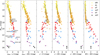 |
Fig. 1. Colours vs. absolute zPS1 magnitude diagrams of metal-poor T dwarf candidates (blue crosses), using trigonometric parallaxes obtained from this work and from the literature, zPS1 photometry from this work and from Zhang et al. (2023) and IR photometry from the literature. The parallax of W1810 comes from Lodieu et al. (2022). For the Accident (black cross and arrow), the parallax comes from (Kirkpatrick et al. 2021a). For comparison, field M, L, T dwarfs with trigonometric parallaxes from Pan-STARRS1 3π survey (Best et al. 2018) are plotted as yellow stars, orange squares, and red dots, respectively. Y dwarfs with zPS1 photometry (corrected from z′) from Lodieu et al. (2013) and Martín et al. (2024), and parallaxes from Kirkpatrick et al. (2019) are plotted as purple triangles. W1217 is a T9+Y2 system, so it is plotted as a mixture of red dot and purple triangle. |
In summary, we confirm the sub-luminosity of three more T subdwarfs: Wolf 1130C, W1553, and W2217. These objects seem to follow the extreme T subdwarf W1810, lying to the blue of the sequence in the following colours: zPS1−J and W1−W2; and to the red in the colours zPS1−W1 and J−W1. We also have another three possible subdwarfs: Ross 19B, W0422, and W2014 in these colour-magnitude diagrams. We observe that the Y subdwarf candidate, the Accident, has an upper limit of the absolute zPS1 magnitude fainter than the current limit for Y dwarfs.
J−H and J−W2 colours do not seem to be good metallicity indicators. Solar-metallicity objects have larger relative J−H colour dispersions probably due to smaller wavelength interval between two bands. With respect to the J−W2 colour, most of metal-poor objects lie on the solar-metallicity sequence. We are going to discuss more about the colours in the next sub-section.
3.2. Colour–colour diagrams
As an update to Fig. 1 in our previous work (Zhang et al. 2023), Figs. 2 and 3 present the colour–colour diagrams of W1−W2 versus zPS1−W1 and J−W2 versus zPS1−W1 for all the objects, with 8508 solar-metallicity M dwarfs, 800 L dwarfs, and 42 T dwarfs from Pan-STARRS1 with and without trigonometric parallaxes (Best et al. 2018), four Y0 dwarfs W0146, W0410, W1738, W2056, a Y2 dwarf W1828, and the T9+Y0 binary W1217. We added the zPS1−W1 limit of the Y4 dwarf WISE J085510.83−071442.5 (Luhman 2014) which is the coldest brown dwarf discovered so far (Beamín et al. 2014; Luhman et al. 2024). There are also 39 L subdwarfs with photometric errors smaller than 0.2 mag in z, J, W1, and W2 bands (Zhang et al. 2018). Three objects, WISEA J001354.40+063448.1, WISEA J083337.81+005213.8, and ULAS J092605.47+083516.9 (included in the previous work) were retained here (Zhang et al. 2023).
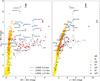 |
Fig. 2. Updated W1−W2 vs. zAB−W1 and J−W2 vs. zAB−W1 colour–colour diagrams with more metal-poor T, Y dwarf candidates compared to the one of Zhang et al. (2023). All the metal-poor T dwarf candidates are labelled with blue crosses and arrows and the Accident is labelled with the black cross and arrow. We over-plotted solar-metallicity M, L, and T sequences from Pan-STARRS (yellow stars, orange squares and red dots, respectively), L subdwarfs (olive squares), four Y0 dwarf, a Y2 dwarf, the Y4 dwarf (purple triangles), and a T9+Y0 system (red dot mixed with purple triangle). All Y dwarfs were identified with CatWISE photometry. Error bars are included for all sources, except for M and L dwarfs. We also show three iso-metallicity curves from the low-metallicity theoretical model LOWZ (Meisner et al. 2021) with parameters: log g = 5.0, log10Kzz = 2, solar C/O ratio 0.55 in both diagrams. From left to right, the effective temperature of the model decreases from 1600 K to 500 K, with a step of 100 K and 50 K above and under 1000 K, respectively. |
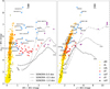 |
Fig. 3. Same as Fig. 2 but with three iso-metallicity curves from the theoretical model SONORA Elf Owl with parameters: log g = 5.0, log10Kzz = 2, and solar C/O ratio in both diagrams. From left to right, the effective temperature of the model decreases from 1500 K to 300 K, with a step of 100 K, 50 K, and 25 K at the temperature above 1000 K, between 600–1000 K and below 600 K, respectively. |
We compared the observations with synthetic photometry derived using filter profiles downloaded from the Spanish Virtual Observatory (SVO) service (Rodrigo et al. 2012; Rodrigo & Solano 2020) and theoretical spectra from the low-metallicity ultracool LOWZ models (Meisner et al. 2021) and the SONORA Elf Owl substellar atmosphere models for T and Y dwarfs (Mukherjee et al. 2024, 2023a,b). We used the following parameters: a high surface gravity log(g) = 5.0, a medium vertical mixing log10Kzz = 2, and a solar C/O ratio of 0.55 for both the LOWZ and the SONORA model. The LOWZ models provide spectra down to metallicity −2.5 dex while the SONORA models only reach to −1.0 dex. The solar-metallicity field dwarf sequence more or less follows the trend of the two sets of models.
Both the LOWZ and the SONORA models predict bluer W1−W2 colours and redder J−W2 colours for lower metallicity objects in the 500–1000 K temperature range. This is clear for the Accident, since it has a significantly bluer W1−W2 colour and a redder J−W2 colour than field Y dwarfs. For the rest of metal-poor T dwarf candidates, they do not tend to concentrate in a smaller W1−W2 interval.
The LOWZ model predicts a zPS1−W1 colour between 4 to 5.5 mag for objects between 500 K and 1600 K (black line in Fig. 2). The LOWZ models predict that for low metallicity (−2.0 dex) the temperature gradient is mainly responsible for the redward shift of the zPS1−W1 colour from 4 to 5 mag. The SONORA model predicts a much stronger temperature dependence than the LOWZ model. The SONORA model also predicts a stable zPS1−W1 colour for hotter objects no matter the metallicity, which contradicts the observations.
We have inferred that the LOWZ models tend to under-estimate the suppression of the zPS1-band flux, caused by the low metallicity. This is also the case for the SONORA models, but only for hotter objects or early-T dwarfs.
On the other hand, the behaviour of the zPS1−W1 colour of subdwarfs is similar to that of the J−W1 colour. Unlike the zPS1−W1 vs. W1−W2 diagram, the observations agree with model predictions in the J−W1 versus W1−W2 diagram (we only plot the LOWZ models in Fig. 4). The LOWZ and SONORA models predict that the J−W1 colours get significant redder for objects cooler than about 1000 K, when the metallicity decreases, and the temperature is the main driver for the metal-poor objects to have the J−W1 colours shifted redward. However, the hotter end of both models (1300–1600 K) exhibits the same problem in the J−W1 colours as in zPS1−W1. Also, they do not accurately reproduce the observed L subdwarfs or the extreme cold solar-metallicity Y2 and Y4 dwarfs. Solar-metallicity T dwarfs exhibit greater dispersion across the spectral type in the J−W1 colour (around 2 mag) compare to the zPS1−W1 colour (around 1.5 mag) In Fig. 4, the spectral types of each metal-poor object are shown, but no clear temperature gradient is evident.
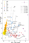 |
Fig. 4. W1−W2 vs. J−W1 colour–colour diagrams of all metal-poor T dwarf candidates (blue crosses and arrows) in Table A.1 and in Zhang et al. (2023). The Accident is shown as the black cross and arrow. We also include the solar-metallicity M, L, and T sequences from Pan-STARRS as yellow stars, orange squares, and red dots, respectively, along with L subdwarfs (olive squares), four Y0 dwarf, a Y2 dwarf, the Y4 dwarf (purple triangles), and a T9+Y0 system (red dot mixed with purple triangle). Error bars are included for all sources, except for M and L dwarfs. We also show five iso-metallicity curves from the low-metallicity theoretical model LOWZ with parameters log(g) = 5.0, log10Kzz = 2, solar C/O ratio 0.55. From left to right of the five curves, the effective temperatures of the model decrease from 1600 K to 500 K, with a step of 100 K and 50 K above and under 1000 K, respectively. |
3.3. zPS1−W1 colour vs. metallicity
In our previous work, we categorised the few candidates into three groups with decreasing metallicity from ≃0 to ≃−1.5 dex, while z−W1 colours increasing from 5 to 7 mag (Zhang et al. 2023). With a larger sample, we can actually see a continuity between the groups and even extensions bluer than 5 mag and much redder than 7 mag.
To see the zPS1−W1 colour trend against the metallicity more clearly, we assigned a coarse metallicity value to each source in our sample. With the exception of Wolf 1130C and Ross 19B, which have spectroscopically determined metallicities derived from their M dwarf primaries, the metallicities of the remaining objects are estimated based on metallicity sub-class classifications obtained through spectroscopy or photometry. This classification of subdwarfs has been a long debated topic and it has not been fully established for T subdwarfs yet because of lack of objects across the whole spectral type range. We adopted the maximum interval of the metallicity value for sub-classes published by different research groups for M and L subdwarfs (Gizis et al. 1997; Lépine et al. 2007; Zhang et al. 2017; Lodieu et al. 2019). Specifically, subdwarfs exhibit metallicities that are primarily between −0.3 and −1.0 dex, extreme subdwarfs between −1.0 and −1.7 dex, and ultra-subdwarfs have below −1.7 dex. We also adopted a metallicity range of +0.3 to −0.3 dex for solar-metallicity field T/Y dwarfs.
For each individual object, we assigned a corresponding metallicity based on the arguments below. A summary of the adopted metallicity for each object is given in Table 4.
-
For the secondaries of comoving pairs, we assumed that all components of a multiple system have a similar chemical composition. There are different measurement of metallicity of the primary Wolf 1130A: −0.62±0.10 dex (Woolf & Wallerstein 2006), −0.70±0.12 dex (Mace et al. 2018), and −0.64±0.17 dex (Rojas-Ayala et al. 2012), but updated to −1.22±0.24 dex (Newton et al. 2014). We adopted a maximum 1-σ range from −0.52 to −1.46 dex for Wolf 1130C.
-
We adopted the iron abundance [Fe/H] of the primary Ross 19A (−0.40±0.12 dex; Schneider et al. 2021) for Ross 19B.
-
Greco et al. (2019) used NIR spectroscopy and classified W0004, W0301, and W1019 as subdwarfs. They do not appear to be very metal-poor objects and they are not sub-luminous in the colour-magnitude diagrams in Fig. 1. We assigned them a metallicity [Fe/H] ranging from −0.3 to −1.0 dex. Meisner et al. (2020a) classified W0422 and W2207 as subdwarfs, but did not specify the metal class. Hence, we adopted a possible range from normal subdwarfs to extreme subdwarfs from −0.3 to −1.7 dex for these two objects.
-
Brooks et al. (2022) listed W0505 as an extreme T subsubdwarf based on its IR colours; hence, we adopted a metallicity ranging from −1.0 to −1.7 dex.
-
Meisner et al. (2021) reported a spectral analysis for W1553, but different models provided different metallicity values, from −0.5 dex to ≲−1.5 dex. We adopted that range.
-
Meisner et al. (2023a) assigned W0156 a metallicity between −0.4 to −0.5 dex because of the adjacent locus to the Ross 19B and the LOWZ model track of −0.5 dex in the colour space. We adopted the same metallicity as that of Ross 19B.
-
For WISEA J041451.67−585456.7, we adopted a range of metallicities from −0.5 to −1.5 dex (Schneider et al. 2020). For WISEA J181006.18−101000.5, we used the range derived by Lodieu et al. (2022), from −1.0 to −2.0 dex.
-
Kellogg et al. (2018) classified W0711 as a subdwarf using its NIR spectrum, its low metallicity is consistent with the thick-disk or halo kinematics. We adopted the metallicity range of subdwarfs, from −0.3 to −1.0 dex.
-
We classified W0738 and W2217 (Meisner et al. 2021) as extreme T subdwarfs based on their large motions and similar colours to the two known extreme T subdwarfs: W1810 and W0414. So we adopted the metallicity range of W1810 and W0414; namely, from −0.5 to −2.0 dex for W0738 and W2217.
-
For W0013 and W0833, Pinfield et al. (2014) estimated a metallicity range from −0.5 to −1.5 dex, based on their peculiar H−W2 colour.
-
Murray et al. (2011) discussed the blue NIR colours and possible halo kinematics of ULAS0926, so we classified it as a subdwarf with a metallicity from −0.3 to −1.0 dex.
-
W0905 and W2014 falls just outside the fiducial colour-colour criteria of extreme subdwarf region proposed by Meisner et al. (2023a). However, W2014 shows a normal spectrum in the Y-, J-, and H-bands. Only its K-band was suppressed (Mace et al. 2013b). Besides, W2014 appears inline with those T subdwarfs only in some of the colour-magnitude diagrams in Fig. 1 and has a J−H colour abnormality. Hence, we assigned a wide metallicity range from subdwarf to extreme subdwarf to W0905, from −0.3 to −1.7 dex; but only a subdwarf metallicity to W2014, from −0.3 to −1.0 dex.
-
The kinematics of W2105 shows that it could be a thick disk/halo dwarf, but the J- and H-band spectra do not show features of low metallicity (Luhman & Sheppard 2014), and Meisner et al. (2023a) excluded it from the list of extreme T subdwarf candidates because its colours put it outside of the locus where extreme T subdwarfs lie. Therefore, we adopted a metallicity from solar 0.0 dex to the most-metal-poor subdwarfs, −1.0 dex.
Adopted metallicity [Fe/H] ranges for metal-poor T/Y dwarf candidates.
We plot the zPS1−W1 colour and metallicity of solar-metallicity field T dwarfs and metal-poor T dwarf candidates in the left panel of Fig. 5. We highlight objects with spectra as circles. We also plot the mean colour and the standard deviation of the colour of solar-metallicity field T dwarfs. The temperature effect for the solar-metallicity T dwarfs on this colour is less than 1 mag (from 4.5 to 5.5 mag). The zPS1−W1 colour does not change significantly at least until the metallicities of W0004, W0301, and W1019. Once the metallicity gets lower than ≈−1.0 dex, the zPS1−W1 colour shoots up and gets drastically redder.
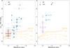 |
Fig. 5. zPS1−W1 colour against metallicity for T and Y dwarfs. The vertical error bars are the photometric errors and the horizontal bars are the adopted metallicity ranges (Table 4). The blue and black crosses are metal-poor T and Y dwarf candidates, respectively. Some upper limit arrows are plotted next to the points to avoid overlapping. The solid blue circle indicates that the object has an NIR spectrum. The two very-late-type metal-poor T dwarf candidates or possible metal-poor Y dwarf candidates Ross 19B and W0156 are indicated by dotted blue circles and are plotted in both panels. The thick red and purple crosses demonstrate the average zPS1−W1 value and dispersion of solar-metallicity T and Y dwarfs, respectively. Five isothermal curves from 500 K to 1300 K from LOWZ model with parameters log(g) = 5.0, log10Kzz = 2, C/O ratio of 0.55 are shown in orange. |
We identify Ross 19B and W0156 as two outliers (dotted blue circles) in the left panel of Fig. 5 with mildly low metallicities but unusually red zPS1−W1 colours. Since the metallicity of W0156 was constrained by Ross 19B (Meisner et al. 2023a), it is not surprising that W0156 aligns with Ross 19B as an outlier. From this point forward, we focus solely on Ross 19B, although our conclusions are applicable to both objects.
Ignoring the possibility of wrong photometry, in the colour-magnitude diagrams, Ross 19B appears extremely sub-luminous compared to solar-metallicity T dwarf counterparts. It is likely to be a colder object, a Y subdwarf, sharing the same chemical component with the primary. It is not contradictory to the photometric spectral type determination: T9.5 ± 1.5 (Schneider et al. 2021). We put both Ross 19B and W0156 into the right panel of Fig. 5, with the mean colour and the standard deviation of the colour of solar-metallicity field Y dwarfs, along with the colour limit of the Accident. The colours of both Ross 19B and W0156 remain between the average colour of the solar-metallicity Y dwarfs and that of the Accident, which is consistent with their mildly low metallicities derived from Ross 19A. However, the Ross 19 system has a projected separation of 9900 au (Schneider et al. 2021). For such a loosely bounded system, it is hard for it to survive dynamically from the Galactic tides given its old age (7.2 Gyr; Schneider et al. 2021). For a binary with a semi-major axis 10 000 au, the simulation for a system with total mass of 1 M⊙ yields a very low probability of surviving for 7 Gyr (Weinberg et al. 1987). We note that the Ross 19 system has a total mass of only 0.4 M⊙.
We provide another possible scenario whereby Ross 19A had captured the B component, which is not necessarily colder, but does have a lower metallicity. The absolute zPS1 magnitude difference between the solar-metallicity sequence and Ross 19B is larger than that between the solar-metallicity sequence and Wolf 1130C in Fig. 1. Wolf 1130C has a similar spectral type as Ross 19B. We therefore hypothesise that Ross 19B could have a much lower metallicity than Wolf 1130C and certainly lower than its primary, Ross 19A. However, the chance for a metal-poor M dwarf to specifically capture a brown dwarf with even lower metallicity is not high either.
It is challenging to assess which case is more probable. In summary, Ross 19B could be colder and be among the metal-poor Y dwarf candidates or it is more metal-poor. The same applies to W0156. Putting these two outliers aside, in the left panel of Fig. 5, we see that objects with zPS1−W1 ≳ 6 mag have a metallicity that is lower or equal than −1.0 dex, namely, extreme subdwarfs. Their spectral types spread from T0 to T8. In other words, the zPS1−W1 colour is observationally a good extreme subdwarf indicator for T dwarfs, which was first proposed by Zhang et al. (2023). This colour could be a metallicity indicator for Y dwarfs according to the right panel of Fig. 5 after adding Ross 19B and W0156, but more observations are needed to confirm this hypothesis.
We plot the LOWZ models in both panels of Fig. 5 once again, using five isothermal lines with metallicity from +0.5 dex to −2.5 dex. The LOWZ models do predict that the zPS1−W1 colour gets redder with decreasing metallicity until −1.0 dex for objects cooler than 900 K (equivalent to mid- to late-T dwarfs). As the temperature decreases, the colour becomes redder in a more pronounced manner. However, the models fail to account for the very red colours observed at lower metallicities for both T and early-Y dwarfs (objects with temperature higher than 500 K).
Our previous work attributed the redder zPS1−W1 colours to the flux increase in the W1 band, due to the weakening of the methane absorption, and expected a saturation at some point Zhang et al. (2023). However, at this moment we still do not appreciate any sign of saturation in the zPS1−W1 colour, although in the case of the current most metal-poor T dwarf with spectroscopic metallicity, W1810, methane is absent or very weak (Lodieu et al. 2022). On the other hand, the absorption wings of alkali metals, especially the sodium NaI and potassium KI resonance doublets at optical wavelengths are broadened in high-gravity atmospheres due to the collision with helium He and molecular hydrogen H2, contributing partly to the suppressed flux in the z passband (Burrows & Volobuyev 2003; Pavlenko et al. 2007; Allard et al. 2016; Phillips et al. 2020). This absorption could be even strengthened due to higher gravity and denser atmospheres in metal-poor environment (Allard et al. 2003, 2023, 2024). These two effects could be underestimated by the LOWZ model, explaining the current discrepancy with the observations.
We further checked the temperature dependence of the zPS1−W1 colour. We plotted the colour of all objects against their spectral type in Fig. 6. We see that the zPS1−W1 colour gets bluer until mid-T dwarfs and then gets redder for solar-metallicity dwarfs. The range of colours remains in a small interval between 4.5 to 5.5 mag. We do not see a clear spectral type dependence for those T subdwarf candidates. We can conclude that the differences in the effective temperature of solar-metallicity T dwarfs will not lead to a extreme red zPS1−W1 colours. Thus, the zPS1−W1 colour can reliably serve as an indicator for extreme T subdwarfs.
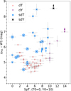 |
Fig. 6. zPS1−W1 colour against spectral type. The solid blue circle indicates that the object has an NIR spectrum. All the objects have a spectral type uncertainty of one sub-type, unless specified differently in Table A.1. We adopted the classification of W1810 as esdT3 in Burgasser et al. (2025). W0156 was classified as a T subdwarf without a sub-type, we assigned it with the same late spectral type as Ross 19B. We assigned a Y0–Y2 range for the Accident, according to its effective temperature. |
3.4. Most metal-poor objects
We see that W0505 and W0738 have exceptionally red zPS1−W1 colours of 8.01 mag and 8.45 mag, respectively. There may exist a population in the colour-colour diagram with zPS1−W1 colours redder than 8.0 mag, represented by ultra subdwarfs (usdTs) with metallicity [Fe/H] below −1.7 dex. However, the WISE photometry of W0505 could be slightly affected by faint background sources; hence, the true zPS1−W1 colour of W0505 could be slightly bluer.
The Accident's extremely low luminosity also points towards a very low effective temperature. The Accident has the reddest zPS1−W1 colour among all the coldest subdwarf candidates and a blue W1−W2 colour suggesting that it could have a very low metallicity. Martín et al. (2024) observed a sharp transition towards bluer z−J colours from 5 to 2 mag from late-T to Y2 dwarfs, respectively, as seen in the colour-magnitude diagram in Fig. 1. The transition agrees with the SONORA solar-metallicity model (Marley et al. 2021). We attribute this effect to the weakening of the very broad KI resonance doublet in the Y dwarf atmosphere, with alkali elements being locked into molecules at low temperatures (Lodders 1999) and carried into deeper layer by rainout processes (Burrows & Sharp 1999). The Accident has a lower limit of 2.2 mag on its zPS1−J, which is consistent with those of solar-metallicity Y dwarfs at the moment.
4. Conclusions
We obtained ground-based trigonometry parallaxes for five metal-poor T dwarf candidates and complemented them with those from the literature. We acquired z-band photometry for another 12 metal-poor T dwarf candidates and five-band optical photometry for the Accident, the only metal-poor Y dwarf candidate to date.
We have confirmed the subdwarf nature of W1553, Wolf 1130C, and W2217, using their loci in the optical-to-IR colour-magnitude diagrams in comparison with their solar-metallicity counterparts and the extreme T subdwarf W1810. We determined possible subdwarf candidates as well, including Ross 19B, W0422, and W2014. We also show that the Y dwarf candidate, the Accident, is more sub-luminous than the current Y dwarf limit. We argue that W0004 and W0301 are not as metal-poor as previously assumed; alternatively, they could be binary candidates based on their loci on the solar-metallicity sequence in the colour-magnitude diagrams. It would be worthwhile to obtain an observation with adaptive optics or interferometry to spatially resolve these binary candidates.
We have provided updated optical-IR colour-colour diagrams, effectively doubling the size of the previous metal-poor T dwarf sample. We strengthened our previous discovery of the relation between the low metallicity and the red zPS1−W1 colour for T dwarfs and we have possibly extended it to Y dwarfs, which has not been predicted by state-of-art models. Combining the three colours, zPS1−W1, J−W1, and W1−W2, may break the metallicity-temperature degeneracy for the coldest populations. This could be useful for identifying future extreme- or even ultra-metal-poor T and Y dwarfs. We confirm the candidacy of W0505 and W0738 to the population of extreme-metal-poor T dwarfs and we propose that Ross 19B and W0156 could be Y subdwarf candidates.
We claim that NIR spectroscopy is highly desirable for determining the metallicity of the extreme T subdwarf candidates W2217, W0505, and W0738. However, due to their faintness, this remains challenging with current ground-based instrumentation, but this could be achievable from space using the JWST. A more practical approach would be obtaining K-band photometry for W0505 and W2217. We also discuss the importance of the spectroscopic determination of the metallicity and temperature of Ross 19B as another benchmark object and an additional anchor point in the diagrams presented in this work. The analysis of the JWST spectrum of the Accident (programme GO 3558, PI A. Meisner; Meisner et al. 2023c) is of extreme importance since it might allow us to synthesise the zPS1 photometry of the only Y subdwarf candidate and measure its metallicity and other physical parameters.
In collaboration with current and future deep optical surveys such as the ESA Euclid mission, Vera Rubin LSST, and Roman space mission, we could launch a tailored survey to search for a specific ultracool population with a given metallicity and effective temperature (Solano et al. 2021; Martín et al. 2021). The main objective is to increase the samples of metal-poor T and Y dwarfs, taking advantage of the complementarity between optical and NIR photometry, as well as astrometric measurements thanks to repeated observations of Vera Rubin LSST and the Euclid deep fields.
Acknowledgments
We thank our referee for providing an insightful report with detailed comments. Funding for this research was provided by the Agencia Estatal de Investigación del Ministerio de Ciencia e Innovación (AEI-MCINN) under grants PID2019-109522GB-C53 and PID2022-137241NB-C41 as well as the European Union (ERC, SUBSTELLAR, project number 101054354). BG acknowledges support from the Polish National Science Center (NCN) under SONATA grant No. 2021/43/D/ST9/0194. Based on observations made with the Gran Telescopio Canarias (GTC), installed at the Spanish Observatorio del Roque de los Muchachos of the Instituto de Astrofísica de Canarias, on the island of La Palma. This work is partly based on data obtained with the instrument HiPERCAM, built by the Universities of Sheffield, Warwick and Durham, the UK Astronomy Technology Centre, and the Instituto de Astrofísica de Canarias. Development of HiPERCAM was funded by the European Research Council, and its operations and enhancements by the Science and Technology Facilities Council. This work is partly based on data obtained with the instrument OSIRIS, built by a Consortium led by the Instituto de Astrofísica de Canarias in collaboration with the Instituto de Astronomía of the Universidad Autónoma de México. OSIRIS was funded by GRANTECAN and the National Plan of Astronomy and Astrophysics of the Spanish Government. This work is partly based on data obtained with the instrument EMIR, built by a Consortium led by the Instituto de Astrofísica de Canarias. EMIR was funded by GRANTECAN and the National Plan of Astronomy and Astrophysics of the Spanish Government. Based on observations collected at Centro Astronómico Hispano en Andalucía (CAHA) at Calar Alto, operated jointly by Instituto de Astrofísica de Andalucía (CSIC) and Junta de Andalucía. Based on observations collected at the European Southern Observatory under ESO programme 113.2688. This research has made use of the Spanish Virtual Observatory (https://svo.cab.inta-csic.es) project funded by MCIN/AEI/10.13039/501100011033/ through grant PID2020-112949GB-I00. This research has made use of the SVO Filter Profile Service “Carlos Rodrigo”, funded by MCIN/AEI/10.13039/501100011033/ through grant PID2020-112949GB-I00. This research has made use of data provided by Astrometry.net. This research has made use of the Simbad and Vizier databases, and the Aladin sky atlas operated at the centre de Données Astronomiques de Strasbourg (CDS), and of NASA's Astrophysics Data System Bibliographic Services (ADS). This research has made use of the NASA/IPAC Infrared Science Archive, which is funded by the National Aeronautics and Space Administration and operated by the California Institute of Technology. This work has used the Pan-STARRS1 Surveys (PS1) and the PS1 public science archive that have been made possible through contributions by the Institute for Astronomy, the University of Hawaii, the Pan-STARRS Project Office, the Max-Planck Society and its participating institutes, the Max Planck Institute for Astronomy, Heidelberg and the Max Planck Institute for Extraterrestrial Physics, Garching, The Johns Hopkins University, Durham University, the University of Edinburgh, the Queen's University Belfast, the Harvard-Smithsonian Center for Astrophysics, the Las Cumbres Observatory Global Telescope Network Incorporated, the National Central University of Taiwan, the Space Telescope Science Institute, the National Aeronautics and Space Administration under Grant No. NNX08AR22G issued through the Planetary Science Division of the NASA Science Mission Directorate, the National Science Foundation Grant No. AST-1238877, the University of Maryland, Eotvos Lorand University (ELTE), the Los Alamos National Laboratory, and the Gordon and Betty Moore Foundation. This publication makes use of data products from the Wide-field Infrared Survey Explorer, which is a joint project of the University of California, Los Angeles, and the Jet Propulsion Laboratory/California Institute of Technology, funded by the National Aeronautics and Space Administration. This project used public archival data from the Dark Energy Survey (DES). Funding for the DES Projects has been provided by the U.S. Department of Energy, the U.S. National Science Foundation, the Ministry of Science and Education of Spain, the Science and Technology Facilities Council of the United Kingdom, the Higher Education Funding Council for England, the National Center for Supercomputing Applications at the University of Illinois at Urbana–Champaign, the Kavli Institute of Cosmological Physics at the University of Chicago, the Center for Cosmology and Astro-Particle Physics at the Ohio State University, the Mitchell Institute for Fundamental Physics and Astronomy at Texas A&M University, Financiadora de Estudos e Projetos, Fundação Carlos Chagas Filho de Amparo à Pesquisa do Estado do Rio de Janeiro, Conselho Nacional de Desenvolvimento Científico e Tecnológico and the Ministério da Ciência, Tecnologia e Inovação, the Deutsche Forschungsgemeinschaft and the Collaborating Institutions in the Dark Energy Survey. The Collaborating Institutions are Argonne National Laboratory, the University of California at Santa Cruz, the University of Cambridge, Centro de Investigaciones Enérgeticas, Medioambientales y Tecnológicas–Madrid, the University of Chicago, University College London, the DES-Brazil Consortium, the University of Edinburgh, the Eidgenössische Technische Hochschule (ETH) Zürich, Fermi National Accelerator Laboratory, the University of Illinois at Urbana-Champaign, the Institut de Ciències de l’Espai (IEEC/CSIC), the Institut de Física d’Altes Energies, Lawrence Berkeley National Laboratory, the Ludwig-Maximilians Universität München and the associated Excellence Cluster Universe, the University of Michigan, the National Optical Astronomy Observatory, the University of Nottingham, The Ohio State University, the OzDES Membership Consortium, the University of Pennsylvania, the University of Portsmouth, SLAC National Accelerator Laboratory, Stanford University, the University of Sussex, and Texas A&M University. The national facility capability for SkyMapper has been funded through ARC LIEF grant LE130100104 from the Australian Research Council, awarded to the University of Sydney, the Australian National University, Swinburne University of Technology, the University of Queensland, the University of Western Australia, the University of Melbourne, Curtin University of Technology, Monash University and the Australian Astronomical Observatory. SkyMapper is owned and operated by The Australian National University's Research School of Astronomy and Astrophysics. The survey data were processed and provided by the SkyMapper Team at ANU. The SkyMapper node of the All-Sky Virtual Observatory (ASVO) is hosted at the National Computational Infrastructure (NCI). Development and support of the SkyMapper node of the ASVO has been funded in part by Astronomy Australia Limited (AAL) and the Australian Government through the Commonwealth's Education Investment Fund (EIF) and National Collaborative Research Infrastructure Strategy (NCRIS), particularly the National eResearch Collaboration Tools and Resources (NeCTAR) and the Australian National Data Service Projects (ANDS). This work made use of Astropy: (http://www.astropy.org) a community-developed core Python package and an ecosystem of tools and resources for astronomy (Astropy Collaboration 2013, 2018, 2022).
References
- Abbott, T. M. C., Abdalla, F. B., Allam, S., et al. 2018, ApJS, 239, 18 [Google Scholar]
- Abbott, T. M. C., Adamów, M., Aguena, M., et al. 2021, ApJS, 255, 20 [NASA ADS] [CrossRef] [Google Scholar]
- Allard, N. F., Allard, F., Hauschildt, P. H., Kielkopf, J. F., & Machin, L. 2003, A&A, 411, L473 [NASA ADS] [CrossRef] [EDP Sciences] [Google Scholar]
- Allard, N. F., Spiegelman, F., & Kielkopf, J. F. 2016, A&A, 589, A21 [NASA ADS] [CrossRef] [EDP Sciences] [Google Scholar]
- Allard, N. F., Myneni, K., Blakely, J. N., & Guillon, G. 2023, A&A, 674, A171 [NASA ADS] [CrossRef] [EDP Sciences] [Google Scholar]
- Allard, N. F., Kielkopf, J. F., Myneni, K., & Blakely, J. N. 2024, A&A, 683, A188 [NASA ADS] [CrossRef] [EDP Sciences] [Google Scholar]
- Appenzeller, I., Fricke, K., Fürtig, W., et al. 1998, Messenger, 94, 1 [Google Scholar]
- Astropy Collaboration (Robitaille, T. P., et al.) 2013, A&A, 558, A33 [NASA ADS] [CrossRef] [EDP Sciences] [Google Scholar]
- Astropy Collaboration (Price-Whelan, A. M., et al.) 2018, AJ, 156, 123 [Google Scholar]
- Astropy Collaboration (Price-Whelan, A. M., et al.) 2022, ApJ, 935, 167 [NASA ADS] [CrossRef] [Google Scholar]
- Bailer-Jones, C. A., Bizenberger, P., & Storz, C. 2000, in Optical and IR Telescope Instrumentation and Detectors, eds. M. Iye, & A. F. Moorwood, SPIE Conf. Ser., 4008, 1305 [Google Scholar]
- Baumeister, H., Bizenberger, P., Bayler-Jones, C. A. L., et al. 2003, in Instrument Design and Performance for Optical/Infrared Ground-based Telescopes, eds. M. Iye, & A. F. M. Moorwood, SPIE Conf. Ser., 4841, 343 [Google Scholar]
- Beamín, J. C., Ivanov, V. D., Bayo, A., et al. 2014, A&A, 570, L8 [NASA ADS] [CrossRef] [EDP Sciences] [Google Scholar]
- Best, W. M. J., Magnier, E. A., Liu, M. C., et al. 2018, ApJS, 234, 1 [Google Scholar]
- Best, W. M. J., Liu, M. C., Magnier, E. A., & Dupuy, T. J. 2020, AJ, 159, 257 [Google Scholar]
- Best, W. M. J., Liu, M. C., Magnier, E. A., & Dupuy, T. J. 2021, AJ, 161, 42 [Google Scholar]
- Brooks, H., Kirkpatrick, J. D., Caselden, D., et al. 2022, AJ, 163, 47 [NASA ADS] [CrossRef] [Google Scholar]
- Burgasser, A. J., Kirkpatrick, J. D., Brown, M. E., et al. 2002, ApJ, 564, 421 [NASA ADS] [CrossRef] [Google Scholar]
- Burgasser, A. J., Kirkpatrick, J. D., Liebert, J., & Burrows, A. 2003a, ApJ, 594, 510 [NASA ADS] [CrossRef] [Google Scholar]
- Burgasser, A. J., Kirkpatrick, J. D., Burrows, A., et al. 2003b, ApJ, 592, 1186 [NASA ADS] [CrossRef] [Google Scholar]
- Burgasser, A. J., Witte, S., Helling, C., et al. 2009, ApJ, 697, 148 [Google Scholar]
- Burgasser, A. J., Schneider, A. C., Meisner, A. M., et al. 2025, ApJ, 982, 79 [Google Scholar]
- Burningham, B., Leggett, S. K., Lucas, P. W., et al. 2010, MNRAS, 404, 1952 [NASA ADS] [Google Scholar]
- Burningham, B., Smith, L., Cardoso, C. V., et al. 2014, MNRAS, 440, 359 [NASA ADS] [CrossRef] [Google Scholar]
- Burrows, A., & Sharp, C. M. 1999, ApJ, 512, 843 [NASA ADS] [CrossRef] [Google Scholar]
- Burrows, A., & Volobuyev, M. 2003, ApJ, 583, 985 [Google Scholar]
- Cepa, J., Aguiar-Gonzalez, M., Gonzalez-Escalera, V., et al. 2000, Optical and IR Telescope Instrumentation and Detectors (SPIE), 4008, 623 [NASA ADS] [CrossRef] [Google Scholar]
- Chabrier, G., Baraffe, I., Phillips, M., & Debras, F. 2023, A&A, 671, A119 [NASA ADS] [CrossRef] [EDP Sciences] [Google Scholar]
- Chambers, K. C., Magnier, E. A., Metcalfe, N., et al. 2016, ArXiv e-prints [arXiv:1612.05560] [Google Scholar]
- Cushing, M. C., Looper, D., Burgasser, A. J., et al. 2009, ApJ, 696, 986 [Google Scholar]
- Cushing, M. C., Kirkpatrick, J. D., Gelino, C. R., et al. 2011, ApJ, 743, 50 [Google Scholar]
- Cutri, R. M., Skrutskie, M. F., van Dyk, S., et al. 2003, The IRSA 2MASS All-Sky Point Source Catalog, NASA/IPAC Infrared Science Archive. http://irsa.ipac.caltech.edu/applications/Gator/ [Google Scholar]
- Delorme, P., Delfosse, X., Albert, L., et al. 2008, A&A, 482, 961 [NASA ADS] [CrossRef] [EDP Sciences] [Google Scholar]
- Dhillon, V. S., Bezawada, N., Black, M., et al. 2021, MNRAS, 507, 350 [NASA ADS] [CrossRef] [Google Scholar]
- Freudling, W., Romaniello, M., Bramich, D. M., et al. 2013, A&A, 559, A96 [NASA ADS] [CrossRef] [EDP Sciences] [Google Scholar]
- Gizis, J. E., Scholz, R. D., Irwin, M., & Jahreiss, H. 1997, MNRAS, 292, L41 [Google Scholar]
- Goodman, S. J. 2021, Res. Notes Am. Astron. Soc., 5, 178 [Google Scholar]
- Greco, J. J., Schneider, A. C., Cushing, M. C., Kirkpatrick, J. D., & Burgasser, A. J. 2019, AJ, 158, 182 [NASA ADS] [CrossRef] [Google Scholar]
- Kellogg, K., Kirkpatrick, J. D., Metchev, S., Gagné, J., & Faherty, J. K. 2018, AJ, 155, 87 [Google Scholar]
- Kirkpatrick, J. D., Gelino, C. R., Cushing, M. C., et al. 2012, ApJ, 753, 156 [NASA ADS] [CrossRef] [Google Scholar]
- Kirkpatrick, J. D., Schneider, A., Fajardo-Acosta, S., et al. 2014, ApJ, 783, 122 [NASA ADS] [CrossRef] [Google Scholar]
- Kirkpatrick, J. D., Martin, E. C., Smart, R. L., et al. 2019, ApJS, 240, 19 [NASA ADS] [CrossRef] [Google Scholar]
- Kirkpatrick, J. D., Marocco, F., Caselden, D., et al. 2021a, ApJ, 915, L6 [NASA ADS] [CrossRef] [Google Scholar]
- Kirkpatrick, J. D., Gelino, C. R., Faherty, J. K., et al. 2021b, ApJS, 253, 7 [Google Scholar]
- Kovács, Z., Mall, U., Bizenberger, P., Baumeister, H., & Röser, H. -J. 2004, in Optical and Infrared Detectors for Astronomy, eds. J. D. Garnett, & J. W. Beletic, SPIE Conf. Ser., 5499, 432 [Google Scholar]
- Kuchner, M. J., Faherty, J. K., Schneider, A. C., et al. 2017, ApJ, 841, L19 [NASA ADS] [CrossRef] [Google Scholar]
- Lang, D., Hogg, D. W., Mierle, K., Blanton, M., & Roweis, S. 2010, AJ, 139, 1782 [Google Scholar]
- Leggett, S. K., Tremblin, P., Phillips, M. W., et al. 2021, ApJ, 918, 11 [NASA ADS] [CrossRef] [Google Scholar]
- Lépine, S., Rich, R. M., & Shara, M. M. 2007, ApJ, 669, 1235 [CrossRef] [Google Scholar]
- Liu, M. C., Dupuy, T. J., Bowler, B. P., Leggett, S. K., & Best, W. M. J. 2012, ApJ, 758, 57 [Google Scholar]
- Lodders, K. 1999, ApJ, 519, 793 [NASA ADS] [CrossRef] [Google Scholar]
- Lodieu, N., Zapatero Osorio, M. R., Martín, E. L., Solano, E., & Aberasturi, M. 2010, ApJ, 708, L107 [Google Scholar]
- Lodieu, N., Béjar, V. J. S., & Rebolo, R. 2013, A&A, 550, L2 [NASA ADS] [CrossRef] [EDP Sciences] [Google Scholar]
- Lodieu, N., Allard, F., Rodrigo, C., et al. 2019, A&A, 628, A61 [NASA ADS] [CrossRef] [EDP Sciences] [Google Scholar]
- Lodieu, N., Zapatero Osorio, M. R., Martín, E. L., Rebolo López, R., & Gauza, B. 2022, A&A, 663, A84 [NASA ADS] [CrossRef] [EDP Sciences] [Google Scholar]
- Luhman, K. L. 2014, ApJ, 786, L18 [Google Scholar]
- Luhman, K. L., & Sheppard, S. S. 2014, ApJ, 787, 126 [Google Scholar]
- Luhman, K. L., Tremblin, P., Alves de Oliveira, C., et al. 2024, AJ, 167, 5 [NASA ADS] [CrossRef] [Google Scholar]
- Mace, G. N., Kirkpatrick, J. D., Cushing, M. C., et al. 2013a, ApJ, 777, 36 [Google Scholar]
- Mace, G. N., Kirkpatrick, J. D., Cushing, M. C., et al. 2013b, ApJS, 205, 6 [Google Scholar]
- Mace, G. N., Mann, A. W., Skiff, B. A., et al. 2018, ApJ, 854, 145 [NASA ADS] [CrossRef] [Google Scholar]
- Mainzer, A., Bauer, J., Cutri, R. M., et al. 2014, ApJ, 792, 30 [Google Scholar]
- Marley, M. S., Saumon, D., Visscher, C., et al. 2021, ApJ, 920, 85 [NASA ADS] [CrossRef] [Google Scholar]
- Marocco, F., Eisenhardt, P. R. M., Fowler, J. W., et al. 2021, ApJS, 253, 8 [Google Scholar]
- Martín, E. L., Zhang, J. Y., Esparza, P., et al. 2021, A&A, 655, L3 [NASA ADS] [CrossRef] [EDP Sciences] [Google Scholar]
- Martín, E. L., Zhang, J. Y., Lanchas, H., et al. 2024, A&A, 686, A73 [NASA ADS] [CrossRef] [EDP Sciences] [Google Scholar]
- Meisner, A. M., Faherty, J. K., Kirkpatrick, J. D., et al. 2020a, ApJ, 899, 123 [NASA ADS] [CrossRef] [Google Scholar]
- Meisner, A. M., Caselden, D., Kirkpatrick, J. D., et al. 2020b, ApJ, 889, 74 [NASA ADS] [CrossRef] [Google Scholar]
- Meisner, A. M., Schneider, A. C., Burgasser, A. J., et al. 2021, ApJ, 915, 120 [NASA ADS] [CrossRef] [Google Scholar]
- Meisner, A. M., Leggett, S. K., Logsdon, S. E., et al. 2023a, AJ, 166, 57 [NASA ADS] [CrossRef] [Google Scholar]
- Meisner, A. M., Caselden, D., Schlafly, E. F., et al. 2023b, Res. Notes Am. Astron. Soc., 7, 36 [Google Scholar]
- Meisner, A., Bardalez Gagliuffi, D. C., Bejar, V., et al. 2023c, The First Spectrum of the Coldest Halo Brown Dwarf, JWST Proposal. Cycle 2, ID. #3558 [Google Scholar]
- Morganson, E., Gruendl, R. A., Menanteau, F., et al. 2018, PASP, 130, 074501 [NASA ADS] [CrossRef] [Google Scholar]
- Mukherjee, S., Fortney, J., Morley, C., et al. 2023a, https://doi.org/10.5281/zenodo.10385821 [Google Scholar]
- Mukherjee, S., Fortney, J., Morley, C., et al. 2023b, https://doi.org/10.5281/zenodo.10381250 [Google Scholar]
- Mukherjee, S., Fortney, J. J., Morley, C. V., et al. 2024, ApJ, 963, 73 [NASA ADS] [CrossRef] [Google Scholar]
- Murray, D. N., Burningham, B., Jones, H. R. A., et al. 2011, MNRAS, 414, 575 [NASA ADS] [CrossRef] [Google Scholar]
- Nakajima, T., Oppenheimer, B., Kulkarni, S., et al. 1995, Nature, 378, 463 [NASA ADS] [CrossRef] [Google Scholar]
- Newton, E. R., Charbonneau, D., Irwin, J., et al. 2014, AJ, 147, 20 [Google Scholar]
- Oke, J. B. 1974, ApJS, 27, 21 [Google Scholar]
- Onken, C. A., Wolf, C., Bessell, M. S., et al. 2024, PASA, 41, e061 [NASA ADS] [CrossRef] [Google Scholar]
- Park, R. S., Folkner, W. M., Williams, J. G., & Boggs, D. H. 2021, AJ, 161, 105 [NASA ADS] [CrossRef] [Google Scholar]
- Pavlenko, Y. V., Zhukovska, S. V., & Volobuev, M. 2007, Astron. Rep., 51, 282 [CrossRef] [Google Scholar]
- Phillips, M. W., Tremblin, P., Baraffe, I., et al. 2020, A&A, 637, A38 [NASA ADS] [CrossRef] [EDP Sciences] [Google Scholar]
- Pinfield, D. J., Gomes, J., Day-Jones, A. C., et al. 2014, MNRAS, 437, 1009 [Google Scholar]
- Rebolo, R., Osorio, M., & Martín, E. 1995, Nature, 377, 129 [NASA ADS] [CrossRef] [Google Scholar]
- Rodrigo, C., & Solano, E. 2020, XIV.0 Scientific Meeting (virtual) of the Spanish Astronomical Society, 182 [Google Scholar]
- Rodrigo, C., Solano, E., & Bayo, A. 2012, SVO Filter Profile Service Version 1.0, IVOA Working Draft 15 October 2012 [Google Scholar]
- Rojas-Ayala, B., Covey, K. R., Muirhead, P. S., & Lloyd, J. P. 2012, ApJ, 748, 93 [Google Scholar]
- Sanghi, A., Liu, M. C., Best, W. M. J., et al. 2023, ApJ, 959, 63 [NASA ADS] [CrossRef] [Google Scholar]
- Saumon, D., Bergeron, P., Lunine, J. I., Hubbard, W. B., & Burrows, A. 1994, ApJ, 424, 333 [NASA ADS] [CrossRef] [Google Scholar]
- Schneider, A. C., Cushing, M. C., Kirkpatrick, J. D., et al. 2015, ApJ, 804, 92 [Google Scholar]
- Schneider, A. C., Burgasser, A. J., Gerasimov, R., et al. 2020, ApJ, 898, 77 [NASA ADS] [CrossRef] [Google Scholar]
- Schneider, A. C., Meisner, A. M., Gagné, J., et al. 2021, ApJ, 921, 140 [Google Scholar]
- Scholz, R. D. 2010, A&A, 510, L8 [NASA ADS] [CrossRef] [EDP Sciences] [Google Scholar]
- Sivarani, T., Lépine, S., Kembhavi, A. K., & Gupchup, J. 2009, ApJ, 694, L140 [Google Scholar]
- Solano, E., Gálvez-Ortiz, M. C., Martín, E. L., et al. 2021, MNRAS, 501, 281 [Google Scholar]
- Stetson, P. B. 1987, PASP, 99, 191 [Google Scholar]
- Tody, D. 1986, in Instrumentation in Astronomy VI, ed. D. L. Crawford, SPIE Conf. Ser., 627, 733 [NASA ADS] [CrossRef] [Google Scholar]
- Tody, D. 1993, in Astronomical Data Analysis Software and Systems II, eds. R. J. Hanisch, R. J. V. Brissenden, & J. Barnes, ASP Conf. Ser., 52, 173 [Google Scholar]
- Weinberg, M. D., Shapiro, S. L., & Wasserman, I. 1987, ApJ, 312, 367 [NASA ADS] [CrossRef] [Google Scholar]
- Woolf, V. M., & Wallerstein, G. 2006, PASP, 118, 218 [Google Scholar]
- Zhang, Z. H., Pinfield, D. J., Gálvez-Ortiz, M. C., et al. 2017, MNRAS, 464, 3040 [NASA ADS] [CrossRef] [Google Scholar]
- Zhang, Z. H., Galvez-Ortiz, M. C., Pinfield, D. J., et al. 2018, MNRAS, 480, 5447 [NASA ADS] [CrossRef] [Google Scholar]
- Zhang, Z. H., Burgasser, A. J., Gálvez-Ortiz, M. C., et al. 2019, MNRAS, 486, 1260 [Google Scholar]
- Zhang, J. Y., Lodieu, N., & Martín, E. L. 2023, A&A, 678, A105 [NASA ADS] [CrossRef] [EDP Sciences] [Google Scholar]
Appendix A: Target information
List of metal-poor T and Y dwarf candidates in our work separated by astrometric and photometric samples.
Appendix B: Astrometric observation log
Logs of the Omega2000 observations of five metal-poor T dwarf candidates.
Appendix C: Astrometry for five metal-poor T dwarf candidates
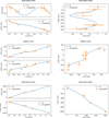 |
Fig. C.1. Left: Observed relative astrometry separated in RA and Dec against the relative time of the reference epoch (0.0 year). Right: Observed relative astrometry together in RA and Dec. |
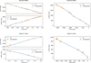 |
Fig. C.1. Continued. |
Appendix D: Photometric observation log
Logs of new optical observations of the Accident and the other 11 metal-poor T dwarf candidates.
Appendix E: GTC & VLT optical images of metal-poor T and Y dwarf candidates
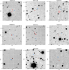 |
Fig. E.1. 45″×45″DES, GTC/OSIRIS, and VLT/FORS2 z-band images of the fields of all the targets with conventional orientation (up is north and left is east). The blue dots are the object positions at the previous epochs published by other authors (Table A.1), and the red ellipses are the projected positions where those targets are supposed to be on the dates of the observations according to their proper motions from the literature in Table A.1. Parallax effects are negligible. The two semi-axes of the ellipses show the errors of projected position in RA and Dec, based on proper motion uncertainties and the time difference between the two epochs. All the objects have been detected. The correct positions of W0156 and W0711 are indicated with the red arrows. |
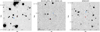 |
Fig. E.1. Continued. |
 |
Fig. E.2. 30″×30″GTC/HiPERCAM quintuple-band optical images of the Accident field with red circles indicating the expected position at the HiPERCAM epoch, compared with HST F110W image (right bottom) with blue circle indicating the Accident at the HST observation epoch. The Accident was not detected in any of the bands. |
All Tables
Revised astrometry of W0156 and W0711 with the astrometry rms, the centroid errors, and the pixel sizes.
New optical photometry and published IR photometry of the Accident, and other 12 metal-poor T dwarf candidates.
List of metal-poor T and Y dwarf candidates in our work separated by astrometric and photometric samples.
Logs of new optical observations of the Accident and the other 11 metal-poor T dwarf candidates.
All Figures
|
Fig. 1. Colours vs. absolute zPS1 magnitude diagrams of metal-poor T dwarf candidates (blue crosses), using trigonometric parallaxes obtained from this work and from the literature, zPS1 photometry from this work and from Zhang et al. (2023) and IR photometry from the literature. The parallax of W1810 comes from Lodieu et al. (2022). For the Accident (black cross and arrow), the parallax comes from (Kirkpatrick et al. 2021a). For comparison, field M, L, T dwarfs with trigonometric parallaxes from Pan-STARRS1 3π survey (Best et al. 2018) are plotted as yellow stars, orange squares, and red dots, respectively. Y dwarfs with zPS1 photometry (corrected from z′) from Lodieu et al. (2013) and Martín et al. (2024), and parallaxes from Kirkpatrick et al. (2019) are plotted as purple triangles. W1217 is a T9+Y2 system, so it is plotted as a mixture of red dot and purple triangle. |
| In the text | |
|
Fig. 2. Updated W1−W2 vs. zAB−W1 and J−W2 vs. zAB−W1 colour–colour diagrams with more metal-poor T, Y dwarf candidates compared to the one of Zhang et al. (2023). All the metal-poor T dwarf candidates are labelled with blue crosses and arrows and the Accident is labelled with the black cross and arrow. We over-plotted solar-metallicity M, L, and T sequences from Pan-STARRS (yellow stars, orange squares and red dots, respectively), L subdwarfs (olive squares), four Y0 dwarf, a Y2 dwarf, the Y4 dwarf (purple triangles), and a T9+Y0 system (red dot mixed with purple triangle). All Y dwarfs were identified with CatWISE photometry. Error bars are included for all sources, except for M and L dwarfs. We also show three iso-metallicity curves from the low-metallicity theoretical model LOWZ (Meisner et al. 2021) with parameters: log g = 5.0, log10Kzz = 2, solar C/O ratio 0.55 in both diagrams. From left to right, the effective temperature of the model decreases from 1600 K to 500 K, with a step of 100 K and 50 K above and under 1000 K, respectively. |
| In the text | |
|
Fig. 3. Same as Fig. 2 but with three iso-metallicity curves from the theoretical model SONORA Elf Owl with parameters: log g = 5.0, log10Kzz = 2, and solar C/O ratio in both diagrams. From left to right, the effective temperature of the model decreases from 1500 K to 300 K, with a step of 100 K, 50 K, and 25 K at the temperature above 1000 K, between 600–1000 K and below 600 K, respectively. |
| In the text | |
|
Fig. 4. W1−W2 vs. J−W1 colour–colour diagrams of all metal-poor T dwarf candidates (blue crosses and arrows) in Table A.1 and in Zhang et al. (2023). The Accident is shown as the black cross and arrow. We also include the solar-metallicity M, L, and T sequences from Pan-STARRS as yellow stars, orange squares, and red dots, respectively, along with L subdwarfs (olive squares), four Y0 dwarf, a Y2 dwarf, the Y4 dwarf (purple triangles), and a T9+Y0 system (red dot mixed with purple triangle). Error bars are included for all sources, except for M and L dwarfs. We also show five iso-metallicity curves from the low-metallicity theoretical model LOWZ with parameters log(g) = 5.0, log10Kzz = 2, solar C/O ratio 0.55. From left to right of the five curves, the effective temperatures of the model decrease from 1600 K to 500 K, with a step of 100 K and 50 K above and under 1000 K, respectively. |
| In the text | |
|
Fig. 5. zPS1−W1 colour against metallicity for T and Y dwarfs. The vertical error bars are the photometric errors and the horizontal bars are the adopted metallicity ranges (Table 4). The blue and black crosses are metal-poor T and Y dwarf candidates, respectively. Some upper limit arrows are plotted next to the points to avoid overlapping. The solid blue circle indicates that the object has an NIR spectrum. The two very-late-type metal-poor T dwarf candidates or possible metal-poor Y dwarf candidates Ross 19B and W0156 are indicated by dotted blue circles and are plotted in both panels. The thick red and purple crosses demonstrate the average zPS1−W1 value and dispersion of solar-metallicity T and Y dwarfs, respectively. Five isothermal curves from 500 K to 1300 K from LOWZ model with parameters log(g) = 5.0, log10Kzz = 2, C/O ratio of 0.55 are shown in orange. |
| In the text | |
|
Fig. 6. zPS1−W1 colour against spectral type. The solid blue circle indicates that the object has an NIR spectrum. All the objects have a spectral type uncertainty of one sub-type, unless specified differently in Table A.1. We adopted the classification of W1810 as esdT3 in Burgasser et al. (2025). W0156 was classified as a T subdwarf without a sub-type, we assigned it with the same late spectral type as Ross 19B. We assigned a Y0–Y2 range for the Accident, according to its effective temperature. |
| In the text | |
|
Fig. C.1. Left: Observed relative astrometry separated in RA and Dec against the relative time of the reference epoch (0.0 year). Right: Observed relative astrometry together in RA and Dec. |
| In the text | |
|
Fig. C.1. Continued. |
| In the text | |
|
Fig. E.1. 45″×45″DES, GTC/OSIRIS, and VLT/FORS2 z-band images of the fields of all the targets with conventional orientation (up is north and left is east). The blue dots are the object positions at the previous epochs published by other authors (Table A.1), and the red ellipses are the projected positions where those targets are supposed to be on the dates of the observations according to their proper motions from the literature in Table A.1. Parallax effects are negligible. The two semi-axes of the ellipses show the errors of projected position in RA and Dec, based on proper motion uncertainties and the time difference between the two epochs. All the objects have been detected. The correct positions of W0156 and W0711 are indicated with the red arrows. |
| In the text | |
|
Fig. E.1. Continued. |
| In the text | |
|
Fig. E.2. 30″×30″GTC/HiPERCAM quintuple-band optical images of the Accident field with red circles indicating the expected position at the HiPERCAM epoch, compared with HST F110W image (right bottom) with blue circle indicating the Accident at the HST observation epoch. The Accident was not detected in any of the bands. |
| In the text | |
Current usage metrics show cumulative count of Article Views (full-text article views including HTML views, PDF and ePub downloads, according to the available data) and Abstracts Views on Vision4Press platform.
Data correspond to usage on the plateform after 2015. The current usage metrics is available 48-96 hours after online publication and is updated daily on week days.
Initial download of the metrics may take a while.