| Issue |
A&A
Volume 698, June 2025
|
|
|---|---|---|
| Article Number | A98 | |
| Number of page(s) | 22 | |
| Section | Astrophysical processes | |
| DOI | https://doi.org/10.1051/0004-6361/202452796 | |
| Published online | 03 June 2025 | |
Attempt to use traveling pulsar wind nebula modeling on the enigmatic LHAASO dumbbell-like structure
1
School of Physics and Astronomy, Sun Yat-sen University, No. 2 Daxue Road, 519082 Zhuhai, China
2
Center for Astro-Particle Physics, University of Johannesburg, P.O. Box 524 Auckland Park 2006, South Africa
⋆ Corresponding authors: This email address is being protected from spambots. You need JavaScript enabled to view it.
; This email address is being protected from spambots. You need JavaScript enabled to view it.
Received:
29
October
2024
Accepted:
9
April
2025
Abstract
Context. The first Large High Altitude Air Shower Observatory (LHAASO) catalog presents six enigmatic ultra-high-energy (UHE) γ-ray sources with lonely > 25 TeV emission being detected, which are indicated as 1LHAASO: J0007+5659u, J0206+4302u, J0212+4254u, J0216+4237u, J1740+0948u, and J1959+1129u. No counterparts of the six sources have been observed except two energetic pulsars, PSR J0218+4232 and PSR J1740+1000. Among them, 1LHAASO: J0206+4302u, J0212+4254u, and J0216+4237u are connected on the significance map and constitute a dumbbell-like structure. They are close in position and show a similar spectral shape, suggesting a physical association among them.
Aims. To explain the origin of the six LHAASO sources, especially the intriguing dumbbell-like structure, we conducted leptonic and hadronic modeling research according to our multiwavelength and multimessenger study. For the dumbbell-like structure, models with traveling pulsar wind nebulae (PWNe) were considered.
Methods. The multiwavelength and multimessenger study was based on the Fermi-LAT, Swift-XRT, Planck, CfA 12CO survey, and IceCube neutrino datasets. In the traveling PWN modeling research, we assumed an isotropic and homogeneous diffusion condition and discussed the influence of the diffusion coefficient, distance, and proper motion velocity.
Results. We do not discover any counterparts in the multiwavelength and multimessenger study except the two known pulsars. The traveling PWN modeling attempt with a single PWN appears to be implausible for explaining the dumbbell-like structure, as the diffusion coefficient needs to be much lower than the Bohm limit. We also explored a double traveling PWNe model, and it could account for the results of the LHAASO observations. However, the probability of the occurrence of this explanation is significantly lower than that of a conventional triple PWNe explanation. Furthermore, according to our model, the only known pulsar, PSR J0218+4232, is unlikely to be associated with the dumbbell-like structure in an isotropic and homogeneous diffusion environment. The expected teraelectronvolt emission of this pulsar is far from explaining even the eastern part of the structure.
Key words: gamma rays: general / diffusion / neutrinos / radiation mechanisms: non-thermal
© The Authors 2025
 Open Access article, published by EDP Sciences, under the terms of the Creative Commons Attribution License (https://creativecommons.org/licenses/by/4.0), which permits unrestricted use, distribution, and reproduction in any medium, provided the original work is properly cited.
This article is published in open access under the Subscribe to Open model. This email address is being protected from spambots. You need JavaScript enabled to view it. to support open access publication.
1. Introduction
As one of the state-of-the-art γ-ray and cosmic ray (CR) detectors, the Large High Altitude Air Shower Observatory (LHAASO) located at Daocheng site, Sichuan province, with altitude of 4410 m, possesses an excellent detection ability in the ultra-high-energy (UHE) band and has expanded the way to discover new UHE γ-ray sources. LHAASO covers energies from 100 GeV to 1 EeV (di Sciascio & LHAASO Collaboration 2016) and achieves sensitivity below 1 × 10⁻¹² erg cm−2 s−1 sr−1 at teraelectronvolt energies (Neronov & Semikoz 2020). It consists of three main components: The Water Cherenkov Detector Array (WCDA) for teraelectronvolt γ-ray detection, The Kilometer Squared Array (KM2A) for detecting γ-ray above 10 TeV, and a Wide Field-of-view atmospheric Cherenkov Telescope Array (WFCTA) mainly for CR detection (Cao et al. 2025). Recently, the LHAASO Collaboration has presented its first catalog of γ-ray sources, reporting ten sources without 1–25 TeV γ-photons detected by WCDA, but with emissions ranging from 25 TeV to above 100 TeV observed by KM2A (Cao et al. 2024). The experimental data are fit by a power-law function, with the fixed reference energy set at 50 TeV (Cao et al. 2024). To avoid the complex background, our work focuses on the six lonely > 25 TeV point-like sources located outside the Galactic plane, which are 1LHAASO: J0007+5659u, J0206+4302u, J0212+4254u, J0216+4237u, J1740+0948u, and J1959+1129u (the prefix 1LHAASO is omitted hereafter). For an overview, the position and spectral information of the sources are presented in Table 1. If these lonely > 25 TeV sources are Geminga-like pulsar wind nebula (PWN) halos, their electron cutoff energies will be far beyond 100 TeV. An even more intriguing aspect is that the sources J0206+4302u, J0212+4254u, and J0216+4237u appear to be spatially linked, forming an extended, dumbbell-like structure on the significance map, and they exhibit a similar spectral shape with an index of approximately 2.5. So far, only two energetic pulsars, PSR J0218+4232 and PSR J1740+1000, have been observed in the vicinity of the six LHAASO sources. Here, PSR J0218+4232 is a millisecond pulsar located near J0216+4237u – the eastern source constituting the dumbbell-like structure. However, no physical associations between the structure and the pulsar can be confirmed due to the relatively large position offset (Cao et al. 2024) and the low predicted teraelectronvolt emission according to the observation from the Fermi Large Area Telescope (Fermi-LAT) and Major Atmospheric Gamma Imaging Cherenkov (MAGIC) (Acciari et al. 2021). PSR J1740+1000 is a middle-aged radio pulsar spatially close to J1740+0948u with a position offset of approximately 0 2. Due to the scarcity of observational data, the physical association between J1740+0948u and PSR J1740+1000 is still unclear. These mysteries on the six LHAASO UHE sources motivate us to investigate their potential origins, which may suggest the existence of new physical mechanisms.
Overview of the six UHE γ-ray sources detected solely by LHAASO-KM2A (Cao et al. 2024), which are the focus of this study.
Among the six LHAASO sources, the intriguing dumbbell-like structure comprising J0206+4302u, J0212+4254u, and J0216+4237u has attracted much attention. We attempt to use the proper motion of a central pulsar powering a PWN to explain its origin and study the traveling PWN model under the isotropic and homogeneous diffusion condition. The central pulsar can either be a known pulsar or a hypothetical one. Zhang et al. (2021) has discussed the impact of a pulsar’s proper motion on the morphology of its γ-ray halo. The results suggest that it is difficult to use the proper motion of a middle-aged pulsar with common distance and proper motion velocity to account for an extended structure. As a further step in research, we have explored a broader parameter space for the model with a single traveling PWN and studied the multiple traveling PWNe model, as well as the probabilities of occurrence for different scenarios.
In this work, to discover the origin of the six LHAASO sources listed in Table 1, we conducted a multiwavelength and multimessenger study with the aim of checking if there are any possible counterparts of the sources observed in other energy bands. The results are presented in Sect. 2 and some details about data analysis are provided in Appendix A. Based on the constraints set by the multiwavelength and multimessenger study, we performed leptonic and hadronic modeling research on the six sources. The best-fit models are presented in Sect. 3, while the corner plots illustrating the models’ ability to explain the data are given in Appendix B. The expected neutrino flux in the hadronic scenario compared with the sensitivity of the next-generation neutrino observatory IceCube-Gen2 is shown in Appendix C. Our traveling PWN modeling attempt within an isotropic and homogeneous diffusion environment, where our aim was to explain the intriguing dumbbell-like structure, is discussed in Sect. 4. We explored the influence of the diffusion coefficient, distance, and proper motion velocity on the final morphology of γ-ray emission. Using the appropriate parameters, we studied models involving a single traveling PWN, two traveling PWNe, and three PWNe, along with their respective probabilities of occurrence. Finally, the conclusion and discussion are given in Sect. 5.
2. Multiwavelength and multimessenger study
2.1. Fermi-LAT dataset
Fermi-LAT was launched into space on June 11, 2008. It is an all-sky γ-ray spatial observatory covering energies from 20 MeV to above 300 GeV (Abdo et al. 2009), with a typical sensitivity of ∼10−12 erg cm−2 s−1 for observation of ten years (Funk et al. 2013). To investigate the morphology of the six LHAASO UHE sources in the lower energy band, we analyzed ten years of data recorded by Fermi-LAT from 2014 January 1 to 2024 January 1 with energies ranging from 300 MeV to 300 GeV. As a result, at the exact locations of the six LHAASO sources, we did not obtain abundant observational data and the γ-ray fluxes of the six sources acquired by the maximum likelihood analysis had error bars larger than the true values. The analysis was conducted by using the publicly available toolkit Fermitools. Since no accurate γ-ray fluxes of the six sources could be extracted from Fermi-LAT dataset, we calculated the upper limits of spectral energy distribution (SED) and used them to constrain the leptonic and hadronic modeling fits discussed in Sect. 3.
To examine the γ-ray sources observed by Fermi-LAT, the test statistic (TS) maps of the six LHAASO sources were also generated with the gttsmap function. Figures 1(a)–(d) present the TS maps corresponding to all the fourth Fermi-LAT catalog sources, the so-called 4FGL sources (Abdollahi et al. 2020), in the vicinity of the six LHAASO sources. We found two 4FGL sources within the 0 5 radius region centered on each LHAASO source. They can be confirmed as the two known pulsars PSR J0218+4232 and PSR J1740+1000, respectively1. Figures 1(e)–(h) show the residual TS maps with all 4FGL sources removed, indicating that no other significant sources appear to be associated with the six LHAASO sources in the energy range of 300 MeV to 300 GeV. Details regarding the maximum likelihood analysis and TS map generating are provided in Appendix A.1.
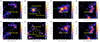 |
Fig. 1. Fermi TS maps within the 5° radius ROIs around the six LHAASO UHE sources. Panels (a)–(d) show TS maps where the nearby 4FGL sources associated with the LHAASO sources are retained. Yellow dashed circles with a radius of 0 |

2.2. Swift-XRT dataset
The Swift Gamma-Ray Explorer is a spatial observatory designed to make prompt multiwavelength observations of gamma-ray bursts (GRBs) and GRB afterglows. The integrated X-ray telescope on the Swift satellite (Swift-XRT) enables it to precisely locate the positions of GRBs with a few arcsecond accuracy within 100 s of the burst onset (Burrows et al. 2005). The Swift-XRT covers an energy range from 0.2 keV to 10 keV, and its sensitivity is 2 × 10⁻¹⁴ erg cm−2 s−1 in 104 s (Burrows et al. 2005). We searched for X-ray sources spatially close to the six LHAASO UHE sources (position offset < 0 3) within the Swift-XRT dataset. As a result, no such source was observed2. Furthermore, among the six sources, Swift-XRT observations were exclusively available within the 0
 3 radius region of interest (ROI) centered on J0206+4302u3. These data with exposure time of 1577.1 s were used to set constraints on SEDs of the six sources in the kiloelectronvolt band as no abundant efficient photons were detected. The obtained upper limits were 7.0 × 10⁻¹⁴ erg cm−2 s−1 at 1.5 keV and 6.1 × 10⁻¹³ erg cm−2 s−1 at 8.1 keV. Appendix A.2 presents more details about the data processing.
2.3. Planck dataset
The Planck satellite, launched on 2009 May 14, is a third-generation space experiment aiming to study the cosmic microwave background (CMB). It covers the observation wavelength from 350 μm to 1 cm and has a good angular resolution of ∼5 arcmin (Tauber et al. 2010).
We hoped to find counterparts, especially molecular clouds (MCs), of the six LHAASO UHE sources in the far infrared band with Planck observations. The up-to-date Planck all-sky map at 857 GHz, obtained from the Planck Public Data Release 3 is shown in Fig. 2. The original data are presented in the hierarchical equal-area isolatitude pixelization (HEALPix) fits table. This pixelization produces a subdivision of a spherical surface in which each pixel covers the same surface area as every other pixel. The raw HEALPix fits table was reprojected into a standard fits table in the world coordinate system (WCS) using the astronomical image toolkit Montage with conventional processing (Jacob et al. 2009), and the data within 10° × 10° ROIs centered on the six sources were extracted for more detailed analyses4. As indicated by the yellow dashed circles in Fig. 2, we did not find significant evidence of counterparts in proximity to these sources, except for J0007+5659u. The exact environment of this source needs to be further identified with carbon monoxide (CO) observations.
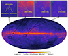 |
Fig. 2. Planck all-sky map at 857 GHz. The map is presented in Galactic coordinates, and the color bar is plotted in logarithmic scale. The zoomed-in views of 10° × 10° ROIs centered on the six sources are presented at the top of the figure. The yellow dashed circles indicate the positions of labeled sources. |
The Planck catalog of compact sources was also checked. However, we did not find source with position offset to the six sources less than 0 3. The catalog can be accessed via the NASA/IPAC Infrared Science Archive official website5.
2.4. CfA 12CO survey dataset
The MCs can provide abundant protons for the inelastic interaction with CR protons, the so-called proton–proton (p–p) interactions, which can result in high-energy γ-ray and neutrino emission (De Sarkar & Gupta 2022). The results of Planck observations can be a reference of whether there exist MCs. However, a more accurate and efficient way to trace MCs is to observe the 12CO J = 1-0 transition line at 115 GHz (Su et al. 2019). We examined the moment-masked (Dame 2011) data of the recent 12CO survey covering the entire northern sky using the CfA 1.2 m telescope and its twin instrument in Chile (Dame & Thaddeus 2022)6. Since the six LHAASO UHE sources are located far from the Galactic plane, this 12CO survey is the only one with publicly available data we can find that directly observed the 115 GHz 12CO line, meanwhile, covering all these six sources. The coverage of the local standard of rest (LSR) velocity is ±47.1 km s−1 and the velocity resolution is 0.65 km s−1. The angular resolution and typical noise fluctuation are 0 25 and 0.18 K, respectively (Dame & Thaddeus 2022).
The moment-masked data can be divided into 146 12CO brightness temperature maps with different LSR velocities. We first checked each 12CO brightness temperature map and found that only the LHAASO source J0007+5659u appears to have a thin MC nearby. The other five sources with larger galactic latitudes were unlikely to be associated with significant MCs. Figure 3 presents the LSR velocity integrated 12CO brightness temperature maps in the vicinity of the six LHAASO sources to clearly show the result, which is consistent with the Planck observations. More details on data analysis are provided in Appendix A.3.
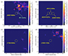 |
Fig. 3. Results of 12CO survey around the six LHAASO UHE sources. The data in panel (a) was integrated with a LSR velocity coverage from –4.9 km s−1 to 1.6 km s−1, covering the MC in proximity to J0007+5659u. For the data in panels (b)–(d), the LSR velocity integrating range was ±47.1 km s−1, reaching the limitation of this survey (Dame & Thaddeus 2022). The positions of the six LHAASO sources are marked by yellow dashed circles with radius of 0 |

The MC proposed to be associated with J0007+5659u covers a sky region of approximately 0 75 × 0
 75. The 12CO spectrum of this MC is shown in Fig. A.1 of Appendix A.3. With a Gaussian fitting, the obtained central LSR velocity was −1.83 ± 0.02 km s−1. Based on this result, the expected distance of the MC can be calculated online with a Bayesian approach in which sources are assigned to spiral arms according to their galactic longitudes, latitudes, and LSR velocities with respect to arm signatures seen in CO and HI surveys (Reid et al. 2016, 2019)7. The result was 0.70 ± 0.04 kpc with a probability of 72%. The mean H2 column density
  of the MC calculated by adopting the 12CO-to-H2 conversion factor of 2 × 1020 cm−2 (K km s−1)−1 (Bolatto et al. 2013) was 1.98 ± 0.57 × 1020 cm−2. Assuming a symmetric spatial distribution of the MC, the mean particle number density
  of the MC can be calculated with (Rani et al. 2023)
 (1)
(1)
where M(H2) and  are the mass and equivalent radius of the MC, respectively. The term μpmp = 2.72mp stands for the mean molecular weight, while mp represents the mass of proton. Using the area, distance, and mean H2 column density
  of the MC previously obtained,
  calculated from Eq. (1) was 10.50 ± 3.08 cm−3.
2.5. IceCube neutrino dataset
High-energy neutrinos are the key to answer whether the γ-ray sources are hadronic or leptonic origins. Together with the multiwavelength observations, from radio to γ-rays, they may shed light on the intrinsic properties of the Galactic sources and their environments.
IceCube neutrino observatory is a kilometer-scale neutrino experiment located at the south pole with 5160 digital optical modules deployed under ice. It was fully constructed on December 18, 2010, and has been collecting data ever since (Aartsen et al. 2017). For the first time, IceCube detected high-energy neutrinos coming from extraterrestrial origins (Aartsen et al. 2013; IceCube Collaboration 2013). Recent years, IceCube has found evidence for neutrino sources, such as TXS 0506+056, NGC1068, and Galactic plane (IceCube Collaboration 2018a,b, 2022; IceCube Collaboration 2023). Some correlation studies of IceCube neutrino and LHAASO sources have been performed, such as the works done by Abbasi et al. (2023), Fang & Halzen (2024), and Li et al. (2024).
We examined the IceCube high-energy starting events (HESE) data release of 12 years. The dataset contains 164 events that are reconstructed based on the latest ice model via DirectFit (Yuan & Chirkin 2024). As a result, we did not find significant association with an offset angle of 2° for these six LHAASO sources. Within the public data release of neutrino track-like events between April 6, 2008 and July 8, 2018, we did not observe significant excess. Therefore, the upper limits were obtained based on the information of exposure time, effective area, and atmospheric background rate at the level of 1 × 10⁻⁹ erg cm−2 s−1 sr−1 for the dumbbell-like structure (Aartsen et al. 2020; IceCube Collaboration 2021).
3. Modeling research
3.1. Leptonic modeling
As observed by the High-Altitude Water Cherenkov Observatory (HAWC) in 2017, the Geminga pulsar (PSR J0633+1746) is surrounded by a prominent teraelectronvolt γ-ray halo, characterized by a hard spectral index of approximately 2.34 (Abeysekara et al. 2017). Notably, the energy range and spectral index of the γ-ray halo around Geminga closely resemble those of the six enigmatic UHE sources detected by LHAASO. This similarity provides a compelling basis to consider Geminga as a reference leptonic model for interpreting the six LHAASO sources.
The relativistic wind generated by a rapid rotation pulsar like Geminga can accelerate the ambient particles, including electrons, and finally forms a bubble of shocked relativistic particles, the so-called PWN (Gaensler & Slane 2006). For relativistic electrons, there are three typical cooling mechanisms – synchrotron radiation, inverse Compton (IC) scattering, and bremsstrahlung (Blumenthal & Gould 1970; Ghisellini et al. 1988; Baring et al. 1999). All of these cooling mechanisms can lead to the emission of photons with various wavelengths. Most of the photons in the kiloelectronvolt band are generated by synchrotron radiation, which originates from relativistic electrons propagating through the ambient magnetic field. Furthermore, with UHE electrons and a strong magnetic field, the energies of photons emitted from this mechanism can be up to gigaelectronvolt (Bednarek & Bartosik 2003). On the other hand, IC scattering between relativistic electrons and the ambient radiation field is a major contributor to high-energy γ-ray emission. The radiation field in IC scattering can be CMB, far-infrared or near-infrared radiation, and visible light (Popescu et al. 2017; Zhang et al. 2021). The energy spectrum of this radiation mechanism can be extended up to the teraelectronvolt range. Also, the bremsstrahlung caused by the collision between relativistic electrons and other particles can contribute to the emission of teraelectronvolt γ-photons, while in general its γ-photon flux is significantly lower than that of IC scattering (Bednarek & Bartosik 2003).
Considering all of the three electron cooling mechanisms mentioned above and assuming Geminga PWN as the reference counterpart, we studied the leptonic origins of the six LHAASO sources. The γ-ray source modeling package GAMERA (Hahn 2015), developed by the Max Planck Institute for Nuclear Physics in Heidelberg (MPIK), was used to calculate the leptonic spectra. The injection electrons of PWN were assumed to satisfy a power-law spectrum with an exponential cutoff. The function can be written as
 (2)
(2)
where Ee denotes the energy of injection electron, αe and Ec are the spectral index and cutoff energy, which are free parameters in our leptonic modeling research. The normalization factor Ne depends on the total energy We of PWN electrons. The relationship between Ne and We is
 (3)
(3)
In our research, We was assumed to be 1.23 × 1045 erg, corresponding to 0.01% of the total spin-down energy of Geminga (Fang et al. 2018). The minimum and maximum energy of the PWN electrons  and
and  were set to be 0.1 GeV and 10 PeV to match the KM2A data. Consulting the approach in work LHAASO Collaboration (2025), the magnetic field strength associated with the six sources was set to 1 μG for calculating the intensity of synchrotron radiation, aligning with the X-ray observation results from Swift-XRT. This is a reasonable value in Galactic halo (Jansson & Farrar 2012). Following Popescu et al. (2017) and Zhang et al. (2021), the radiation fields in IC scattering were assumed to be CMB (with temperature of 2.73 K and energy density of 0.25 eV cm−3), far-infrared radiation (with temperature of 40 K and energy density of 1 eV cm−3), near-infrared radiation (with temperature of 500 K and energy density of 0.4 eV cm−3), and visible light (with temperature of 3500 K and energy density of 1.9 eV cm−3). The ambient particle number density around the PWN for bremsstrahlung calculation was assumed to be 0.1 cm−3 (De Sarkar & Gupta 2022). The distance d from the PWN to Earth was left free, as it determines the total flux intensity when We was kept fixed.
In summary, the free parameters to fit in our model were αe, Ec, and d. The Markov chain Monte Carlo (MCMC) method was used for fitting (Geyer 1992). In this procedure, the input and output in our model were the energy of γ-photons and the corresponding SED, respectively. The experimental data to fit were the fitting KM2A SEDs of the six sources presented by the LHAASO catalog (Cao et al. 2024). For leptonic modeling, the upper limits of SEDs in different energy bands based on Fermi-LAT (see Sect. 2.1), Swift-XRT (see Sect. 2.2), and WCDA (Cao et al. 2024) datasets were adopted to constrain the fitting. A punishment on likelihood while the output of model exceeding the upper limit was added to the likelihood function of the MCMC fitting. Before running the fitting, the scientific calculation toolkit Scipy was used to obtain the start point of the Markov chain. Each chain contained 2000 steps while the first 200 steps were regarded as burn-in steps. The entire calculation and fitting were performed under the Python3 environment.
Figure 4 shows the results of our leptonic modeling research. The corner plots showing the posterior probability distribution function (PDF) of each fitting parameter in the model are given in Fig. B.1 of Appendix B. According to these corner plots, the MCMC fittings have reached convergence. The best-fit αe, Ec, and d are presented in Table 2. For all of the six sources, the best-fit spectral indexes are within the range of 1.6–1.9, while the best-fit cutoff energies are above 100 TeV. These best-fit values are reasonable for electron injection of a PWN (Gaensler & Slane 2006; de Oña Wilhelmi et al. 2022), implying a scenario where the six LHAASO sources may originate from energetic PWNe like Geminga. The relatively large uncertainties in the best-fit values of Ec and d listed in Table 2 stem from the scarcity of observational data, as the multiwavelength and multimessenger study has only provided upper limits. This represents the primary limitation of our modeling research.
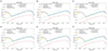 |
Fig. 4. Results of leptonic modeling research. Panel (a) shows the result of J0007+5659u. The solid blue line represents the total SED of γ-ray generated by leptonic interactions. The dashed and dotted lines in different colors are the SEDs contributed from synchrotron radiation, IC scattering, and bremsstrahlung. The pointing down arrows stand for the upper limits obtained from the observations of Swift-XRT, Fermi-LAT, and WCDA. The expected sensitivity of 3 × 10⁴ seconds’ observation with EPIC-pn of XMM-Newton has been shown by the thick golden line. The fitting SED of KM2A data with error bar is displayed by a butterfly plot filled in gray. Panels (b)–(f) are the results of J0206+4302u, J0212+4254u, J0216+4237u, J1740+0948u, and J1959+1129u, respectively. |
Best-fit parameters in leptonic modeling research.
In Fig. 4, the expected sensitivity of 3 × 10⁴ seconds’ observation with the EUROPEAN PHOTON IMAGING CAMERA (EPIC) integrated on XMM-Newton in the energy range of 0.5–10 keV is also presented8. One can see that even with a weak magnetic field strength of 1 μG, the sensitivity limit of XMM-Newton can reach the predicted X-ray SED in our leptonic model, while a proper exposure time is required. That means, it is possible for some sensitive X-ray telescopes (e.g., XMM-Newton) to detect the potential X-ray fluxes from the six LHAASO sources, which is essential to determine whether these sources belong to leptonic origins, such as the IC scattering between UHE electrons from PWN and CMB. Thus, we anticipate further research in the X-ray band with state-of-the-art X-ray telescopes.
3.2. Hadronic modeling
In addition to the three cooling mechanisms of relativistic electrons appeared in the last subsection, p–p interactions also play a significant role in the production of UHE γ-rays. In the category of astronomy, p–p interactions conventionally happen between accelerated CR protons and cold MC protons. Inelastic collisions among these protons produce light mesons, which can decay into γ-photons through reactions such as π0 → γγ and η → γγ. This process is always accompanied by the production of neutrinos. Thus, if an UHE γ-ray source is confirmed as hadronic origin, the study combined with neutrino detection can be very helpful in revealing the exact physical mechanisms behind it.
As previously mentioned, for the p–p interaction, the MC which provides cold protons is always essential. According to Sects. 2.3 and 2.4, we can only find a thin MC in the vicinity of J0007+5659u. Although the position offset of approximately 0 5 may decrease the possibility of J0007+5659u being associated with the MC, we still explored a model of p–p interaction to evaluate the possibility that this source belongs to the hadronic scenario. In the model, we assumed J0007+5659u to originate from the p–p interaction between injection CR protons and cold protons from the MC indicated in Fig. 3(a). The modeling research was also performed with the GAMERA toolkit (Hahn 2015). The injection CR protons were assumed to have a simple power-law spectrum in the form of
 (4)
(4)
where Ep denotes the energy of injection CR proton. As in the leptonic scenario, the normalization factor Np also depends on the total energy Wp of the injection CR protons. Since there was no information on the source responsible for the acceleration of CR protons, Wp was set as a free parameter in our model. The term αp is the spectral index. It was also left free in the model. The maximum energy  of CR protons was chosen to be the CR knee energy of ∼3.16 PeV, while the minimum energy
  was another free parameter.
In addition to the energy spectrum of CR protons, the total inelastic cross section is also of great importance in the p–p interaction. In the GAMERA toolkit we adopted, it is expressed as (Kafexhiu et al. 2014)
 (5)
(5)
In Eq. (5), the cross section is presented in units of millibarn. The energy dependent dimensionless term L can be written as L = Ep/(0.2797 GeV).
As previously discussed, there were three free parameters to fit in our p–p interaction modeling research – Wp, αp, and  . To simplify the calculation, we assumed that Wp satisfies the formula Wp = 1 × 10Γ1 erg and
  satisfies the formula
  TeV. Thus, the fitting parameters were transformed into three dimensionless indexes Γ1, Γ2, and αp. As in Sect. 3.1, the input and output in our p–p interaction model were the energy of γ-photons and the corresponding SED, respectively. An MCMC method with each chain containing 2000 steps (the first 200 steps were burn-in steps) was adopted, while the fitting KM2A SED of J0007+5659u was regarded as experimental data. The upper limits of SEDs in different energy bands based on Fermi-LAT (see Sect. 2.1) and WCDA (Cao et al. 2024) datasets were used to constrain the output of the model. The upper limits of neutrino flux obtained from the IceCube dataset (see Sect. 2.5) were much higher than those of Fermi-LAT and WCDA. Thus, they were not involved in the fitting. During the processing, the distance and mean particle number density of the MC were the same as presented in Sect. 2.4.
Figure 5 shows the result of our hadronic modeling research on J0007+5659u compared with that in the leptonic scenario. Notably, the γ-ray SED generated by p–p interaction seems more consistent with the fitting SED of KM2A. Also, the corner plot showing the posterior PDF of each fitting parameter in the model is presented in Fig. B.2 of Appendix B. The MCMC fitting in hadronic model is converged, as shown by the corner plot. The best-fit Γ1 is  , which results in Wp of
  erg. Adopting the assumption of symmetric spatial distribution of the MC, which is previously discussed in Sect. 2.4, the required energy density Up of the injection CR protons is
  eV cm−3. This value is approximately 1.7 times lower than the average value in the Milky Way, while higher than that of the Large Magellanic Cloud (Yoast-Hull et al. 2016). The best-fit Γ2 is
  , corresponding to
  of
of  TeV. The best-fit αp is
  , which is reasonable for CR protons (De Sarkar & Gupta 2022). The sensitivity limit of XMM-Newton with an exposure time of 3 × 10⁴ seconds, which can reach the X-ray flux predicted by our leptonic model, is also presented in Fig. 5. We anticipate observations of the exact location of J0007+5659u with current X-ray telescopes, such as XMM-Newton, to be highly useful in determining whether this source has a leptonic or hadronic origin, as the hadronic scenario does not predict X-ray emission.
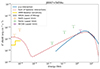 |
Fig. 5. Best-fit result of the hadronic model for J0007+5659u, fit to the multiwavelength upper limits, compared with the best-fit result of the leptonic model. The solid blue line represents the SED of γ-ray generated by p–p interaction. The dashed line in red stands for the total SED of γ-ray generated by leptonic interactions. The pointing down arrows denote the upper limits of SED according to the observations of Swift-XRT, Fermi-LAT, and WCDA. Also, the expected sensitivity of 3 × 10⁴ seconds’ observation with EPIC-pn of XMM-Newton has been shown by the thick golden line. The fitting SED of KM2A data with error bar is displayed by a butterfly plot filled in gray. |
The minimum energy of the injection protons expected in our hadronic model is relatively high. This might imply a scenario where a supernova remnant (SNR) possessing a long Sedov time (De Sarkar & Gupta 2022) is associated with the MC in proximity to J0007+5659u. The SNR traps low-energy CR protons in a small region and leads to the lonely > 25 TeV emission from J0007+5659u. However, our examination within the online high-energy SNR catalog (Ferrand & Safi-Harb 2012) appeared not to support this explanation, as no SNR spatially close to J0007+5659u was found9. Searching for some other CR proton accelerator candidates such as blazars (Murase et al. 2012) and active galactic nuclei (George et al. 2008) in this sky region, along with a CO survey possessing higher angular resolution, are required for further research.
As previously mentioned, the generation of γ-photons in p–p interaction is always accompanied by the production of neutrinos via the decay of pions and muons. Thus, neutrino detection is also essential for identifying the origin of a γ-ray source and can provide helpful supplementary information about the source. According to our hadronic modeling research, the expected neutrino SED from J0007+5659u is approximately an order of magnitude below the sensitivity limit of IceCube-Gen2 after ten years of observation at 10 TeV, and about two orders of magnitude lower at 100 TeV. It seems unlikely to observe the neutrino fluxes emitted from this source at current stage, even the hadronic origin has been confirmed. However, with improved technologies, there are still prospects of detecting associated neutrinos with some other proposed next-generation neutrino observatories, such as TRIDENT (Ye et al. 2023) and NEON (Zhang et al. 2024). The details of neutrino SED calculation are provided in Appendix C.
4. Traveling PWN modeling attempt
One of the most attractive discoveries presented by the LHAASO catalog is the dumbbell-like structure comprising J0206+4302u, J0212+4254u, and J0216+4237u10 The similarities in position and spectral shape of the three sources suggest a physical association among them. The low UHE γ-ray source density at such high galactic latitude makes this assumption more plausible. Some previous studies have attempted to explain the physical association proposing mechanisms such as the asymmetric propagation of UHE electrons caused by turbulent magnetic fields surrounding pulsars to account for this structure and identifying PSR J0218+4232 as a potential counterpart (Bao et al. 2024a,b). Furthermore, the relativistic jet from a microquasar, which can form a double-peaked γ-ray morphology (H. E. S. S. Collaboration et al. 2024), is also a potential explanation for the generation of the dumbbell-like structure. However, the current multiwavelength and multimessenger observation on this structure have not shown enough evidence. In this section, we attempt to use the traveling PWN model with one traveling PWN, two traveling PWNe, and three PWNe under the isotropic and homogeneous diffusion condition to explain the origin of the dumbbell-like structure.
4.1. Single traveling PWN modeling attempt
Firstly, we discuss the hypothesis that the dumbbell-like structure was formed by a single traveling PWN. For this scenario, the model only requires one corresponding pulsar, and its complexity can be significantly reduced, since there is no need to account for the probability of spatial coincidences among multiple pulsars. Similar to the propagation of CR particles, the relativistic electrons accelerated by the central pulsar associated with a PWN undergo spatial diffusion. This process is accompanied by the proper motion of the central pulsar and leaves γ-ray and X-ray filaments. According to the statistical study, a pulsar can travel with a velocity of up to ∼1600 km s−1 (Hobbs et al. 2005). If the distance d between the PWN and Earth is short enough (< 0.5 kpc), with such a proper motion velocity, the significant γ-ray filament is likely to be detected by LHAASO-KM2A and misunderstood as three point-like sources.
The diffusion of electrons accelerated by a pulsar can be described by a diffusion equation (Delahaye et al. 2008, 2010; Fang et al. 2018; Zhang et al. 2021; Fang & Bi 2022):
![Mathematical equation: $$ \begin{aligned} \frac{\partial \psi }{\partial t}-\nabla \cdot [D(E_{e})\nabla \psi ]-\frac{\partial }{\partial E_{e}}[b(E_{e})\psi ]=q(\boldsymbol{r},E_{e},t). \end{aligned} $$](/articles/aa/full_html/2025/06/aa52796-24/aa52796-24-eq66.gif) (6)
(6)
Here, ψ(r, Ee, t) denotes the electron number density per unit energy, D(Ee)≡D0ϵδ is the energy-dependent diffusion coefficient assumed to be isotropic and homogeneous (Zhang et al. 2021; Fang & Bi 2022), D0 represents the normalization factor, and ϵ ≡ Ee/Ed is the dimensionless energy of electron, where Ed = 1 GeV (Delahaye et al. 2008, 2010). The term b(Ee) describes the energy-loss rate of electrons due to synchrotron radiation and IC scattering on cosmic radiation fields (Delahaye et al. 2008). The exact form of b(Ee), considering the Klein-Nishina effect (Nakar et al. 2009), can be written as (Zhang et al. 2021)
![Mathematical equation: $$ \begin{aligned} b(E_{e})&=-\frac{dE_{e}}{dt}\nonumber \\&=\frac{4}{3}\sigma _{T}c\left(\frac{E_{e}}{m_{e}c^{2}}\right)^{2}\left[U_{B}+\frac{U_{\mathrm{ph}}}{\left(1+\frac{4E\epsilon _{0}}{m_{e}^{2}c^{4}}\right)^{3/2}}\right]\nonumber \\&= \frac{4}{3}\sigma _{T}c\epsilon ^{2}\left(\frac{E_{d}}{m_{e}c^{2}}\right)^{2}\left[U_{B}+\frac{U_{\mathrm{ph}}}{\left(1+\frac{4E_{d}\epsilon \epsilon _{0}}{m_{e}^{2}c^{4}}\right)^{3/2}}\right]. \end{aligned} $$](/articles/aa/full_html/2025/06/aa52796-24/aa52796-24-eq67.gif) (7)
(7)
Here, σT is the Thomson cross section, c denotes the velocity of light, and me stands for the mass of electron. The term UB = B2/(2μ0) is the energy density of magnetic field, where B represents the strength of magnetic field and μ0 stands for the permeability of vacuum. The energy density of radiation field is represented by Uph. The term ϵ0 = 2.82kbT is the typical photon energy of the blackbody/graybody target radiation field, as kb and T are the Boltzmann constant and temperature, respectively.
Assuming the PWN to be a constant injection source, the source term q(r, Ee, t) is expected to follow a power-law spectrum with an exponential cutoff
 (8)
(8)
where Γ is the spectral index of injection spectrum, r0 denotes the position of the traveling PWN at t = 0, and v stands for the proper motion velocity of the central pulsar. The normalization factor q0 depends on the total energy of PWN injection, which is denoted by We in the previous text. The relationship between q0 and We is similar to that between Ne and We, as presented in Eq. (3). The We is a fraction η0 of the total spin-down energy W0 of the corresponding pulsar, while W0 satisfies the equation (Gaensler & Slane 2006; Fang & Bi 2022)
 (9)
(9)
Here,  denotes the rotational kinetic energy dissipation rate or called “spin-down luminosity” of the pulsar at t = ta, and ta represents the evolutionary time of the pulsar. In our model, the spin-down luminosity decays with time following Ding et al. (2021), meanwhile, Γ and Ec of the accelerated electrons remain constant through the traveling history. The term τ0 ∼ 10 kyr is the typical spin-down luminosity decay time (Ding et al. 2021).
Based on Eqs. (3), (7), (8), and (9), the full expansion of Eq. (6) can be expressed as
 (10)
(10)
while
![Mathematical equation: $$ \begin{aligned} \frac{1}{\tau _{l}}&=\frac{4}{3}\sigma _{T}c\frac{E_{d}}{m_{e}^{2}c^{4}}\left[U_{B}+\frac{U_{\mathrm{ph}}}{\left(1+\frac{4E_{d}\epsilon \epsilon _{0}}{m_{e}^{2}c^{4}}\right)^{3/2}}\right],\end{aligned} $$](/articles/aa/full_html/2025/06/aa52796-24/aa52796-24-eq72.gif) (11)
(11)
 (12)
(12)
Here, ϵmin and ϵmax represent the constraints on the energy of electrons emitted by PWN. The term γn(t) is a step function, which returns 1 when t ≥ 0.
As the diffusion coefficient is isotropic and homogeneous, we can use the Green’s function method to solve Eq. (10) analytically. For our model, the Green’s function can be written as (Fang & Bi 2022)
![Mathematical equation: $$ \begin{aligned} G(\boldsymbol{r},t\leftarrow \boldsymbol{r}_{s},t_{s}) = \frac{b(\epsilon ^{*})}{b(\epsilon )}\frac{1}{(\pi \lambda ^{2})^{3/2}}{\mathrm{exp}}\left[-\frac{(\boldsymbol{r}-\boldsymbol{r}_{s})^{2}}{\lambda ^{2}}\right], \end{aligned} $$](/articles/aa/full_html/2025/06/aa52796-24/aa52796-24-eq74.gif) (13)
(13)
where rs and ts represent the position and time of an arbitrary electron injection in the Green’s function method. The diffusion length λ and the modified dimensionless energy ϵ* are expressed as follows:
 (14)
(14)
 (15)
(15)
For a free boundary condition, the analytical solution of Eq. (10) based on the Green’s function method can be expressed as
 (16)
(16)
Here, ti = max{t − τl/ϵ, 0} is the injection time, while τl/ϵ = Ee/b(Ee) describes the cooling timescale of the injection electrons (Zhang et al. 2021).
The morphology of PWN electron diffusion, combined with proper motion, depends on several parameters, with the most significant being the diffusion coefficient D(Ee), the distance d, and the proper motion velocity v. Thus, we first explored the influence of varying D0, d, and v. From Eq. (14), one can see that the diffusion length of electron is in direct proportion to  . With a higher D0, the electrons diffuse more rapidly, resulting in a decrease in the local electron number density and a lower γ-ray flux intensity. The parameters d and v mainly influence the evolutionary time ta of the pulsar. To form the > 25 TeV dumbbell-like structure, ta needs to be shorter than the cooling timescale of > 100 TeV electrons which are essential to the generation of > 25 TeV γ-photons. Moreover, d also has impact on the extension size of the source and the γ-ray flux intensity experimentally observed.
The spatial distribution of electron number density per unit energy can be directly calculated by Eq. (16) and transformed into γ-ray flux intensity map with the magnetic field and radiation field model adopted in Sect. 3.1. Figure 6 presents the γ-ray flux intensity maps at 50 TeV corresponding to different values of D0. Here, a pulsar proper motion perpendicular to the line of sight (LOS) was assumed (Zhang et al. 2021), and D0 varied from an extremely low observed value of 4.8 × 1024 cm2 s−1 around HESS J1026–582 (Di Mauro et al. 2020) to the typical value of 6.9 × 1025 cm2 s−1 around Geminga (Fang & Bi 2022). The D0 of 4.8 × 1024 cm2 s−1 is much lower than the Bohm limit (Abeysekara et al. 2017; Mukhopadhyay & Linden 2022). Such a value can only be reached under a strong magnetic turbulence condition (Shalchi 2009; Hussein & Shalchi 2014), which can result in anisotropic diffusion. In Fig. 6, the lower bound of γ-ray SED is set at 1 × 10⁻¹⁶ erg cm−2 s−1. As shown in Fig. 6, with the increase of D0, the rapid diffusion of electrons decrease the local electron number density and consequently diminish the γ-ray flux intensity. This leads to the teraelectronvolt γ-ray blob becoming smaller (due to the SED cut) and dimmer as D0 increases. Thus, for the single traveling PWN scenario, only if the diffusion coefficient is significantly lower than the Bohm limit, the teraelectronvolt γ-photons emitted from the PWN can cover the entire sky region of the dumbbell-like structure as presented in Fig. 6(a).
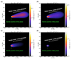 |
Fig. 6. Results of γ-ray flux intensity map at 50 TeV generated for different values of D0. Panels (a)–(d) give the results for D0 = 4.8 × 1024 cm2 s−1, 1.2 × 1025 cm2 s−1, 2.8 × 1025 cm2 s−1, and 6.9 × 1025 cm2 s−1, respectively. For comparing with the physical image shown in the LHAASO catalog, the coordinate system used here is the J2000 equatorial frame. The other parameters adopted in the calculation are d = 0.4 kpc and v = 1600 km s−1. The white arrow indicates the proper motion direction of the pulsar, while the green star marks the current position of the pulsar. |
The γ-ray flux intensity maps at 50 TeV with different values of d are presented in Fig. 7. Also, the direction of pulsar proper motion was assumed to be perpendicular to the LOS. The value of d varied from 0.2 kpc to 0.8 kpc, covering a reasonable range. As in Fig. 6, the lower bound of the γ-ray SED in Fig. 7 is set at 1 × 10⁻¹⁶ erg cm−2 s−1. As shown in the figure, when d is too small, leading to an excessively short ta, the recently injected energetic electrons form a large and bright γ-ray blob. In this case, a double-peaked structure, like the one observed in the LHAASO significance map, cannot be reproduced. With the increase of d, ta can be longer than the cooling timescale of UHE electrons. Due to the cooling of previously injected electrons, the teraelectronvolt γ-ray emission ceases to cover the entire sky region of the dumbbell-like structure. Therefore, the dumbbell-like structure can only be produced by a single pulsar located at an appropriate distance, as demonstrated in Fig. 7(b).
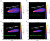 |
Fig. 7. Results of γ-ray flux intensity map at 50 TeV generated for different values of d. Panels (a)–(d) give the results for d = 0.2 kpc, 0.4 kpc, 0.6 kpc, and 0.8 kpc, respectively. The other parameters adopted in the calculation are D0 = 4.8 × 1024 cm2 s−1 and v = 1600 km s−1. |
Finally, the γ-ray flux intensity maps at 50 TeV, generated for different values of v, are shown in Fig. 8. Here, v varied from a common value of 400 km s−1 to the maximum observed value of 1600 km s−1 (Hobbs et al. 2005). As presented in Fig. 8, even with a sufficiently short distance, the pulsar still needs to travel at an extraordinary velocity exceeding 1200 km s−1 to prevent the cooling of UHE electrons, which is essential for generating the observed dumbbell-like structure. As the proper motion velocity increases to 1600 km s−1, the morphology gradually becomes double-peaked.
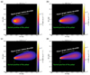 |
Fig. 8. Results of γ-ray flux intensity map at 50 TeV generated for different values of v. Panels (a)–(d) give the results for v = 400 km s−1, 800 km s−1, 1200 km s−1, and 1600 km s−1, respectively. The other parameters adopted in the calculation are D0 = 4.8 × 1024 cm2 s−1 and d = 0.4 kpc. |
Based on our exploration about the impact of D0, d, and v on γ-ray morphology, we set D0 = 4.8 × 1024 cm2 s−1, d = 0.4 kpc, and v = 1600 km s−1 in the single traveling PWN scenario. The above parameters can be regarded as some typical values required for a dumbbell-like structure to be created by a single pulsar. Using these parameters, along with the previously adopted magnetic field and radiation field model, the γ-photon count map for energies exceeding 25 TeV is presented in Fig. 9(a). Here, we assumed that the PWN travel from ( ,
,  ) to (
 ,
,  ) during the evolution. Some other major parameters used are presented in Table 3. The parameter
  reflecting the total energy of injection electrons was adjusted to a proper value that leads to the conformity between the calculated and observed γ-ray flux intensities from the three LHAASO sources. The parameter δ = 0.33 was a typical value predicted by the Kolmogorov’s theory (Fang & Bi 2022). The evolutionary time ta was calculated from the selected values of v and d.
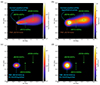 |
Fig. 9. Predicted γ-photon count maps and smoothed significance maps for energies exceeding 25 TeV in the single traveling PWN modeling attempt. Panel (a) shows the γ-photon count map calculated with D0 = 4.8 × 1024 cm2 s−1, d = 0.4 kpc, and v = 1600 km s−1. The blue arrow indicates the proper motion direction of the hypothetical pulsar proposed in our model. Panel (b) shows the predicted significance map seen from LHAASO. The result has been smoothed with the LHAASO PSF at energies above 25 TeV (1 |

Major parameters adopted in the single traveling PWN modeling attempt.
By considering the diffuse Galactic γ-ray emission (GDE) background (Cao et al. 2024) and applying a Gaussian smooth with  , it is not difficult to predict the significance map seen from LHAASO based on the γ-photon count map. The 1σ value used here is similar to that of the LHAASO point-spread function (PSF) at energies above 25 TeV (Cao et al. 2025). Figure 9(b) presents the calculated significance map for energies exceeding 25 TeV. The results demonstrate that, under the assumption of an extremely low diffusion coefficient and an ultra-fast proper motion velocity of the central pulsar, the filament of a single traveling PWN – produced through isotropic and homogeneous diffusion of electrons – can exhibit a double-peaked morphology resembling the dumbbell-like structure observed by LHAASO-KM2A. Comparing Figs. 9(a) and (b), it is evident that the western > 25 TeV blob (J0206+4302u) is formed by the diffused electrons from the central pulsar with higher spin-down luminosity at the early time, meanwhile, the eastern > 25 TeV blob (J0216+4237u) is generated by the fresh PWN electrons recently injected and extended with the LHAASO PSF. However, the necessity of a diffusion coefficient below the Bohm limit under the assumption of isotropic diffusion renders this explanation seemingly implausible. The proper motion of a single pulsar may provide a more valid explanation for certain double-peaked extended structures with smaller scales (angular sizes of approximately 1°) observed in lower energy bands (< 10 TeV).
In Figs. 9(a) and (b), except for the three LHAASO sources, the position of the only known energetic pulsar nearby – PSR J0218+4232 is also marked. Notably, PSR J0218+4232 lies in close proximity to the current position of the hypothetical traveling pulsar proposed in our model. However, based on our calculation, it seems impossible that PSR J0218+4232 is the traveling pulsar required. In the calculation, we adopted a diffusion coefficient of 6.9 × 1025 cm2 s−1, consistent with the value observed around Geminga. This value falls within the one standard deviation range of the statistical results for the diffusion coefficients derived from 27 pulsars (Di Mauro et al. 2020). As reported in the Australia Telescope National Facility (ATNF) pulsar catalog (Manchester et al. 2005), the spin-down luminosity, distance, and proper motion velocity of PSR J0218+4232 used in the calculation were 2.4 × 1035 erg s−1, 3.15 kpc, and 97.48 km s−1, respectively. Some other common values such as the spectral index of 1.4 and the cutoff energy of 800 TeV for injection electrons were also adopted. Figures 9(c)–(d) present the predicted γ-photon count map and the smoothed significance map, respectively. Unsurprisingly, there is no filament produced by this pulsar and only the electrons recently injected can contribute to γ-ray emission, due to its long distance to Earth and slow proper motion velocity. Therefore, under the isotropic and homogeneous diffusion condition, the dumbbell-like structure observed by LHAASO-KM2A appears unlikely to be generated solely by PSR J0218+4232.
4.2. Multiple traveling PWNe modeling attempt
In the previous subsection, we explored the scenario of a single traveling PWN. By adopting extreme parameter values, such as a diffusion coefficient D0 of 4.8 × 1024 cm2 s−1 and a proper motion velocity v of 1600 km s−1, the predicted γ-ray morphology aligns well with the observations from LHAASO-KM2A. However, since this model requires an isotropic diffusion coefficient significantly lower than the Bohm limit, it is nearly unattainable from a physical perspective. If the diffusion coefficient becomes larger, the rapid diffusion of electrons will disrupt the double-peaked morphology, causing the dumbbell-like structure to vanish. Thus, we favor a traveling PWN model involving multiple pulsars to account for the origin of the dumbbell-like structure.
In the analysis, we first assumed PSR J0218+4232 as one of the traveling PWNe in our model, and expected its teraelectronvolt γ-ray emission combined with the contribution from a hypothetical traveling PWN possessing conventional characteristics to form a morphology resembling the dumbbell-like structure. The result is shown in Figs. 10(a)–(b). The calculation was accomplished by adding an extra source term to Eq. (10) and analytically solving the equation with the Green’s function method. The diffusion coefficient was also set as the typical value of 6.9 × 1025 cm2 s−1. All parameters associated with PSR J0218+4232 had the same values as adopted in Sect. 4.1. The hypothetical PWN was assumed to travel from ( ,
,  ) to (
 ,
,  ) during the evolution. The distance d and the proper motion velocity v for its central pulsar were set to 0.4 kpc and 800 km s−1, respectively. All the parameters applied here no longer exhibit extreme values; instead, they fall within reasonable ranges consistent with those of a conventional pulsar. The proper motion velocity of the hypothetical pulsar is relatively fast but still acceptable. As presented in Figs. 10(a)–(b), the teraelectronvolt γ-photons emitted from a conventional pulsar appear unlikely to cover a sky region with an angular size of approximately 3°, due to the cooling of UHE electrons (Zhang et al. 2021). Consequently, the traveling PWN model including PSR J0218+4232 and a conventional pulsar is still far from explaining the origin of the dumbbell-like structure.
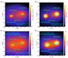 |
Fig. 10. Predicted γ-photon count maps and smoothed significance maps for energies exceeding 25 TeV in the multiple traveling PWNe modeling attempt. Panels (a)–(b) show the γ-photon count map and significance map calculated with the model including PSR J0218+4232 and a hypothetical pulsar. The blue arrow indicates the proper motion direction of the hypothetical pulsar. Panels (c)–(d) show the γ-photon count map and significance map calculated with the model including two hypothetical pulsars. Here, the γ-ray emission from PSR J0218+4232 has been excluded. |
According to the current results, the only known pulsar PSR J0218+4232 can be ruled out under the isotropic and homogeneous diffusion environment. However, this pulsar is still an important potential counterpart of the dumbbell-like structure in some other theories, such as the asymmetric propagation of UHE electrons due to the turbulent magnetic fields around pulsars (Bao et al. 2024a,b). As PSR J0218+4232 had been excluded, we explored the possibility of using two relatively fast-traveling PWNe located at short distances to account for the dumbbell-like structure. One of the PWNe was assumed to travel from ( ,
,  ) to (
 ,
,  ) during the evolution, while the other one was assumed to travel from (
 ,
,  ) to (
 ,
,  ). The major parameters adopted for the two corresponding central pulsars are presented in Table 4. The contribution of PSR J0218+4232 was not considered in this scenario.
Major parameters adopted in the double traveling PWNe modeling attempt.
Figures 10(c)–(d) show the expected γ-photon count map and the smoothed significance map, respectively. Compared with Figs. 10(a)–(b), the γ-ray morphology in the scenario involving two hypothetical pulsars aligns more closely with the observational result of LHAASO-KM2A. For this scenario, both of the two > 25 TeV blobs are generated by the fresh PWN electrons recently injected and extended with the LHAASO PSF while the entire extended structure is a combination of the diffuse filaments left by the two PWNe. As all the parameters applied on the two pulsars possess common values, the double traveling PWNe explanation is physically plausible. However, some strong constraints on the characteristics of the two pulsars are still necessary. As indicated in Table 4, the conditions of short distance and fast travel of the two pulsars are supposed to be satisfied simultaneously. Moreover, to form the dumbbell-like structure, the proper motions of the two pulsars need to be opposite in direction, which significantly reduces the likelihood of this scenario. The probability of this explanation, as well as the more conventional interpretation involving the three LHAASO UHE sources corresponding to three PWNe – whose leptonic modeling has been explored in Sect. 3.1 – will be discussed in more detail in Sect. 4.3.
4.3. Probabilities of occurrence for different scenarios
As previously discussed, to form a dumbbell-like structure as observed by LHAASO-KM2A with isotropic and homogeneous diffusion of PWN electrons, some constraints need to be set on the corresponding central pulsars. Furthermore, since more than one pulsar is required, spatial coincidences among multiple pulsars are also essential. Thus, the probability of occurrence Pk for each scenario can be calculated by
 (17)
(17)
where k is the number of PWN. The terms Pdiff, Pd, and Pv describe the probabilities that the diffusion coefficient, distance, and proper motion velocity fall within their constraint ranges, respectively. The probability of pulsars spatial coincidence by chance is represented by Pc.
For the single traveling PWN model, although the requirement for an isotropic diffusion coefficient below the Bohm limit renders the explanation seemingly improbable, the applied value finds observational support – potentially due to anisotropic diffusion – around HESS J1026–582 (Di Mauro et al. 2020). Consequently, we estimated the likelihood of this scenario. Since the diffusion coefficient around HESS J1026–582 is far outside the one standard deviation interval, the Pdiff in this scenario is much lower than 0.32. The exact result cannot be provided here due to the scarcity of statistical samples. For the multiple traveling PWNe model with two and three pulsars, a conventional diffusion coefficient like the typical value around Geminga can satisfy the requirement of generating the dumbbell-like structure. Thus, no specific constraint on the diffusion coefficient was required, which results in Pdiff = 1.
The radial density profile of Galactic pulsars can be described by a gamma function (Lorimer et al. 2006):
![Mathematical equation: $$ \begin{aligned} \rho (R) = A\left(\frac{R}{R_{\odot }}\right)^{F}{\mathrm{exp}}\left[-C\left(\frac{R-R_{\odot }}{R_{\odot }}\right)\right], \end{aligned} $$](/articles/aa/full_html/2025/06/aa52796-24/aa52796-24-eq101.gif) (18)
(18)
where R represents the galactocentric radius and R⊙ = 8.3 kpc is the distance between the Sun and Galactic center. The values of fitting parameters A, F, and C depend on the model. Along the direction perpendicular to the Galactic plane, the distribution of Galactic pulsars is assumed to satisfy a simple exponential function (Lorimer et al. 2006):
 (19)
(19)
Here, z denotes the height above the Galactic plane. Fitting parameters D and H are also model-dependent. Based on the fundamental geometrical relationship, it is not difficult to extract the Galactic pulsar distribution depending on d via Eqs. (18) and (19). For the scenarios involving one pulsar and two pulsars, we assumed d < 0.5 kpc, while for the triple pulsars scenario, based on the considerations outlined in Sect. 3.1, we implemented a more relaxed constraint of d < 6 kpc. Thus, Pd of the three scenarios with one pulsar, two pulsars, and three pulsars calculated by integrating the profile of d are 0.0327, 0.0327, and 0.4862, respectively. The values of fitting parameters used in the calculation follow the Model C fit in Lorimer et al. (2006).
Based on the statistical result on proper motion velocities of 233 pulsars, the distribution of v is well described by a Maxwellian distribution (Hobbs et al. 2005), which can be written as
 (20)
(20)
where the best-fit 1D root-mean-square σv is 265 km s−1. For the single traveling PWN model, we assumed v > 1200 km s−1. Thus, based on Eq. (20), Pv of this scenario is 0.00013. For the double traveling PWNe model, we assumed v > 600 km s−1 and obtained Pv = 0.1628. In the conventional triple PWNe model, no constraint on v was required. Thus, for this scenario, we have Pv = 1.
At last, we considered the calculation of Pc in multiple traveling PWNe scenarios. The probability of two pulsars accidentally appear in the same sky region with position offset r1 can be expressed as (Mattox et al. 1997)
 (21)
(21)
while
![Mathematical equation: $$ \begin{aligned} r_{0}=[\pi \rho (\dot{\xi })]^{-1/2}. \end{aligned} $$](/articles/aa/full_html/2025/06/aa52796-24/aa52796-24-eq105.gif) (22)
(22)
Here,  represents the number density of local pulsars. Consulting the method used in Cao et al. (2024), we examined the ATNF catalog to check the number of pulsars within a 20° ×5° sky region centered on the exact location of J0212+4254u. Considering the pulsar needs to be energetic enough to be detected by LHAASO-KM2A, a cut at
  erg s−1 kpc−2 was applied during the examination, following Cao et al. (2024). As a result, before the cut on
  , there were four pulsars found within the 20° ×5° sky region, while only two pulsars were left after the cut. The value extracted from the ATNF catalog is merely the number density of observed radio pulsars, which should be corrected to the actual number density of pulsars based on the product of beaming fraction and detection fraction (Johnston et al. 2020). Following Johnston et al. (2020), we assumed a ratio of 0.09 between the number density of observed pulsars and the actual value. Thus,
  around the dumbbell-like structure is ∼765.36 rad−2.
For the double traveling PWNe scenario, based on the separation between the two hypothetical pulsars and  of 765.36 rad−2, Pc can be directly calculated by Eqs. (21) and (22). The result is 0.9814. However, since the two pulsars need to travel in almost opposite directions, this value should be multiplied by the probability of proper motion directions coincidence by chance to acquire the actual Pc. According to our simulation, the appropriate angle between the proper motion directions of the two pulsars to form the dumbbell-like structure is 180 ± 5°. Thus, the actual Pc of this scenario is 0.9814/36 = 0.0273.
The problem will become more complicated in the triple PWNe scenario. We first calculated the probability of accidentally having two pulsars with position offset equal to that between J0206+4302u and J0216+4237u via Eqs. (21) and (22). Afterward, the result was multiplied by the probability of having another pulsar coincidentally appeared in a 0 2 radius circle region (the radius was assumed to be the 1σ value of LHAASO PSF at energies exceeding 25 TeV) centered on the exact location of J0212+4254u, which can be calculated by
![Mathematical equation: $$ \begin{aligned} P(S) = \rho (\dot{\xi })S{\mathrm{exp}}[-\rho (\dot{\xi })S], \end{aligned} $$](/articles/aa/full_html/2025/06/aa52796-24/aa52796-24-eq112.gif) (23)
(23)
where S is the area of the circle region in units of radian2. Consequently, we could obtain the Pc of triple PWNe scenario as 0.0319.
As all the values of different probabilities have been estimated, based on Eq. (17), Pk of the three scenarios with one pulsar, two pulsars, and three pulsars are ≪0.00014%, ∼0.00008%, and ∼0.37%, respectively. As a brief summary, Table 5 presents all the results obtained from our calculation. It is worth noting that, even the conventional triple PWNe model appears to be more complicated, the probability of occurrence for this scenario is still much higher than that of the other two scenarios. The underlying rationale is straightforward. To explain the dumbbell-like structure comprising three UHE sources through either the proper motion of one pulsar or two pulsars in the isotropic and homogeneous diffusion environment would necessitate imposing numerous stringent constraints on the characteristics of pulsars, which can significantly increase the complexity of model and reduce the probability of occurrence. Thus, it might not be a good choice to use the proper motion of a single pulsar, or even several pulsars, to explain such a giant extended structure in the UHE band.
Probabilities of occurrence for different scenarios.
5. Conclusion and discussion
The first LHAASO catalog presents six enigmatic UHE sources solely detected by LHAASO-KM2A (Cao et al. 2024). All of them are located far from the Galactic plane and have no confirmed counterparts. Only two energetic pulsars, PSR J0218+4232 and PSR J1740+1000, are found in proximity to J0216+4237u and J1740+0948u, respectively. A more intriguing aspect is that J0206+4302u, J0212+4254u, and J0216+4237u are spatially linked and share a similar spectral shape. On the significance map, these three sources constitute a dumbbell-like structure.
To reveal the physical mechanisms hiding behind the six LHAASO UHE sources, especially the intriguing dumbbell-like structure, we conducted a multiwavelength and multimessenger study based on the Fermi-LAT, Swift-XRT, Planck, CfA 12CO survey, and IceCube neutrino datasets. As a result, only two γ-ray sources were observed by Fermi-LAT, and they could be identified as the two known pulsars PSR J0218+4232 and PSR J1740+1000. For the X-ray band study based on the Swift-XRT dataset, no abundant efficient photons were detected. Within the Planck and CfA 12CO survey datasets, only the source J0007+5659u appeared to have a thin MC nearby, and we studied the potential hadronic origin of this source. For further research, we expect CO surveys with enhanced angular resolution and LSR velocity coverage. Based on the HESE data release of 12 years and track-like events of ten years within the IceCube neutrino dataset, no neutrino event was found to be associated with the six sources. Moreover, with the RATAN-600 radio telescope, the three sources constituting the dumbbell-like structure were observed at three to five epochs in February and April, 2024. No positive detection was found, and some preliminary results on upper limits were given: J0206+4302u (< 4 mJy), J0218+4232 (< 6 mJy), and J0212+4254u (< 6 mJy). Since the current multiwavelength and multimessenger study has not identified any confirmed counterparts, the origins of these six LHAASO sources remain uncertain.
Based on the results of the multiwavelength and multimessenger study, we performed leptonic and hadronic modeling research on the six LHAASO sources. In the leptonic scenario, we assumed the six sources originated from Geminga-like PWNe whose injection electron spectra satisfy the simple power-law function with an exponential cutoff. Our leptonic model indicated very high exponential cutoff energies (> 100 TeV) for all six sources, which are common for pulsar injection (de Oña Wilhelmi et al. 2022). In the hadronic scenario, we focused on the p–p interaction origin of J0007+5659u, where the CRs were assumed to interact with the MC spatially close to J0007+5659u. The results of the modeling research are physically reasonable. Our model suggests a notable observational implication, namely, that X-ray band observations with sensitive telescopes such as XMM-Newton could provide helpful diagnostic information to determine whether J0007+5659u belongs to leptonic or hadronic origins. Based on the best-fit parameters in the hadronic model, we also calculated the expected neutrino flux from J0007+5659u. The result is significantly below the sensitivity limit of IceCube-Gen2 after ten years of observation. However, there still remains the possibility of detecting associated neutrino fluxes with some other proposed next-generation neutrino observatories such as TRIDENT (Ye et al. 2023) and NEON (Zhang et al. 2024).
For the enigmatic dumbbell-like structure we are most interested in, which is also recognized as three point-like sources in the LHAASO catalog (Cao et al. 2024), we studied a traveling PWN model under the isotropic and homogeneous diffusion condition. We first explored the scenario including only one traveling PWN. We discussed the impact of diffusion coefficient, distance, and proper motion velocity on the final morphology of the γ-ray emission. As a result, we find that to generate a dumbbell-like structure with a single pulsar, the diffusion coefficient has to be much lower than the Bohm limit, while the proper motion velocity needs to be approximately 1600 km s−1. Furthermore, the distance within an appropriate range is also essential. Such extreme preconditions deny the possibility for the only known pulsar, PSR J0218+4232 (which possesses a long distance to Earth and a slow proper motion velocity), to be the assumed traveling PWN in our model. With all the required parameters applied and adopting a typical PWN spin-down evolution history following Ding et al. (2021), we demonstrated that the filament left by the proper motion of a single traveling PWN could exhibit a double-peaked morphology and generate a significance map aligning with the result of LHAASO-KM2A. However, based on the present theories, it is very difficult for electrons to diffuse much slower than Bohm diffusion under the premise of isotropic diffusion. Thus, the single traveling PWN model seems invalid for explaining the origin of such a giant extended structure, which agrees with the results presented in Zhang et al. (2021). As the isotropic and homogeneous diffusion condition is not a constraint on our model, we plan to explore the single traveling PWN scenario under the anisotropic diffusion environment in the future.
We also studied a model including two traveling PWNe. At first, PSR J0218+4232 was involved in the study, but it was later ruled out since the expected teraelectronvolt emission of this pulsar was far from explaining even the eastern part of the dumbbell-like structure. However, if this pulsar is surrounded by a turbulent magnetic field environment, the “mirage source” formed by the asymmetric propagation of electrons (Bao et al. 2024a,b) can lead to a γ-ray morphology resembling the KM2A observation. Thus, this pulsar is still an important potential counterpart of the dumbbell-like structure. Assuming two hypothetical pulsars with relatively fast proper motion velocities and short distances, the double traveling PWNe model could also generate an extended structure aligning well with the dumbbell-like structure observed by LHAASO-KM2A. Since no extreme parameters were applied, we consider this explanation to be acceptable.
The probabilities of occurrence for the two scenarios previously mentioned along with that of the most conventional explanation with the three LHAASO UHE sources corresponding to three PWNe, as discussed in Sect. 3.1, were also estimated. As a result, the probability of occurrence for the triple PWNe scenario is more than three orders of magnitude higher than those of the scenarios requiring fewer PWNe. It is straightforward to see that the stringent constraints on the characteristics of the corresponding central pulsars can significantly increase the complexity of the model and reduce the probability of occurrence, even for the double traveling PWNe scenario. Thus, it appears unreasonable to use the proper motion of a single pulsar or several pulsars to account for a giant extended structure in the UHE band. As the conventional triple PWNe explanation has the highest probability of occurrence, we expect the radio band observation with the Five-hundred-meter Aperture Spherical radio Telescope (FAST) and X-ray band observation with XMM-Newton on the exact locations of J0206+4302u, J0212+4254u, and J0216+4237u can be helpful in revealing the origin of the dumbbell-like structure. Furthermore, we anticipate the up-to-date experimental data from the LHAASO Collaboration can provide more details on the exact morphology and spectral characteristics of the dumbbell-like structure.
Data availability
The LHAASO spectral data (WCDA upper limits and KM2A fitting SEDs with error bars) presented in Figs. 4 and 5 are available at the CDS via anonymous ftp to cdsarc.cds.unistra.fr (130.79.128.5) or via https://cdsarc.cds.unistra.fr/viz-bin/cat/J/A+A/698/A98
For more details, visit the Public List of LAT-Detected Gamma-Ray Pulsars at https://confluence.slac.stanford.edu/display/GLAMCOG/Public+List+of+LAT-Detected+Gamma-Ray+Pulsars
The Swift-XRT 2SXPS catalog at https://www.swift.ac.uk/2SXPS/ was checked.
The data were acquired from https://heasarc.gsfc.nasa.gov/cgi-bin/W3Browse/swift.pl
More details about the HEALPix fits table and Montage processing can be found at http://montage.ipac.caltech.edu/docs/HEALPix/
The data are available at https://lweb.cfa.harvard.edu/rtdc/CO/NorthernSkySurvey/
The sensitivity is based on the XMM-Newton Users Handbook, which can be downloaded from http://xmm-tools.cosmos.esa.int/external/xmm_user_support/documentation/uhb/XMM_UHB.pdf
The significance map on the dumbbell-like structure is presented at the left bottom of Fig. 10 in Cao et al. (2024).
The software can be downloaded from https://heasarc.gsfc.nasa.gov/lheasoft/download.html.
The Galactic value of hydrogen column density can be calculated online at https://www.swift.ac.uk/analysis/nhtot/.
Acknowledgments
We thank the anonymous referee for the constructive comments and suggestions. We thank Ruoyu Liu, Shaoqiang Xi, Sujie Lin, Renfeng Xu, Wenjun Huang, and Sheng Tang for the helpful discussion. We thank Timur Mufakharov and Yulia Sotnikova for the RATAN-600 observation. This work was supported by the National Natural Science Foundation of China (NSFC) Grants No. 12261141691 and No. 12005313. We thank the support from Fundamental Research Funds for the Central Universities, Sun Yat-sen University, No. 24qnpy123.
References
- Aartsen, M. G., Abbasi, R., Abdou, Y., et al. 2013, Phys. Rev. Lett., 111, 021103 [Google Scholar]
- Aartsen, M. G., Ackermann, M., Adams, J., et al. 2017, JInst, 12, P03012 [Google Scholar]
- Aartsen, M. G., Ackermann, M., Adams, J., et al. 2020, Phys. Rev. Lett., 124, 051103 [Google Scholar]
- Abbasi, R., Ackermann, M., Adams, J., et al. 2023, ApJ, 945, L8 [Google Scholar]
- Abdo, A. A., Ackermann, M., Ajello, M., et al. 2009, ApJ, 707, 1310 [NASA ADS] [CrossRef] [Google Scholar]
- Abdollahi, S., Acero, F., Ackermann, M., et al. 2020, ApJS, 247, 33 [Google Scholar]
- Abeysekara, A. U., Albert, A., Alfaro, R., et al. 2017, Science, 358, 911 [NASA ADS] [CrossRef] [Google Scholar]
- Acciari, V. A., Ansoldi, S., Antonelli, L. A., et al. 2021, ApJ, 922, 251 [Google Scholar]
- An, Q., Asfandiyarov, R., Azzarello, P., et al. 2019, Sci. Adv., 5, eaax3793 [NASA ADS] [CrossRef] [Google Scholar]
- Bao, Y., Giacinti, G., Liu, R. Y., Zhang, H. M., & Chen, Y. 2024a, arXiv e-prints [arXiv:2407.02478] [Google Scholar]
- Bao, Y., Liu, R. Y., Giacinti, G., Zhang, H. M., & Chen, Y. 2024b, arXiv e-prints [arXiv:2407.02829] [Google Scholar]
- Baring, M. G., Ellison, D. C., Reynolds, S. P., Grenier, I. A., & Goret, P. 1999, ApJ, 513, 311 [NASA ADS] [CrossRef] [Google Scholar]
- Bednarek, W., & Bartosik, M. 2003, A&A, 405, 689 [NASA ADS] [CrossRef] [EDP Sciences] [Google Scholar]
- Blumenthal, G. R., & Gould, R. J. 1970, Rev. Mod. Phys., 42, 237 [Google Scholar]
- Bolatto, A. D., Wolfire, M., & Leroy, A. K. 2013, ARA&A, 51, 207 [CrossRef] [Google Scholar]
- Burrows, D. N., Hill, J. E., Nousek, J. A., et al. 2005, Space Sci. Rev., 120, 165 [Google Scholar]
- Cao, Z., Aharonian, F., An, Q., et al. 2024, ApJS, 271, 25 [NASA ADS] [CrossRef] [Google Scholar]
- Cao, Z., Aharonian, F., Axikegu, et al. 2025, Astropart. Phys., 164, 103029 [CrossRef] [Google Scholar]
- Funk, S., Hinton, J. A., & CTA Consortium 2013, Astropart. Phys., 43, 348 [NASA ADS] [CrossRef] [Google Scholar]
- Dame, T. M. 2011, arXiv e-prints [arXiv:1101.1499] [Google Scholar]
- Dame, T. M., & Thaddeus, P. 2022, ApJS, 262, 5 [NASA ADS] [CrossRef] [Google Scholar]
- Dame, T. M., Hartmann, D., & Thaddeus, P. 2001, ApJ, 547, 792 [Google Scholar]
- de Oña Wilhelmi, E., López-Coto, R., Amato, E., & Aharonian, F. 2022, ApJ, 930, L2 [CrossRef] [Google Scholar]
- Delahaye, T., Lineros, R., Donato, F., Fornengo, N., & Salati, P. 2008, Phys. Rev. D, 77, 063527 [NASA ADS] [CrossRef] [Google Scholar]
- Delahaye, T., Lavalle, J., Lineros, R., Donato, F., & Fornengo, N. 2010, A&A, 524, A51 [NASA ADS] [CrossRef] [EDP Sciences] [Google Scholar]
- De Sarkar, A., & Gupta, N. 2022, ApJ, 934, 118 [NASA ADS] [CrossRef] [Google Scholar]
- Di Mauro, M., Manconi, S., & Donato, F. 2020, Phys. Rev. D, 101, 103035 [NASA ADS] [CrossRef] [Google Scholar]
- Ding, Y.-C., Li, N., Wei, C.-C., Wu, Y.-L., & Zhou, Y.-F. 2021, Phys. Rev. D, 103, 115010 [Google Scholar]
- di Sciascio, G.& LHAASO Collaboration 2016, Nucl. Part. Phys. Proc., 279-281, 166 [CrossRef] [Google Scholar]
- Enokiya, R., Sano, H., Filipović, M. D., et al. 2023, PASJ, 75, 970 [CrossRef] [Google Scholar]
- Fang, K., & Bi, X.-J. 2022, Phys. Rev. D, 105, 103007 [Google Scholar]
- Fang, K., & Halzen, F. 2024, J. High Energy Astrophys., 43, 140 [Google Scholar]
- Fang, K., Bi, X.-J., Yin, P.-F., & Yuan, Q. 2018, ApJ, 863, 30 [CrossRef] [Google Scholar]
- Ferrand, G., & Safi-Harb, S. 2012, Adv. Space Res., 49, 1313 [Google Scholar]
- Gaensler, B. M., & Slane, P. O. 2006, ARA&A, 44, 17 [Google Scholar]
- George, M. R., Fabian, A. C., Baumgartner, W. H., Mushotzky, R. F., & Tueller, J. 2008, MNRAS, 388, L59 [NASA ADS] [Google Scholar]
- Geyer, C. J. 1992, Stat. Sci., 7, 473 [Google Scholar]
- Ghisellini, G., Guilbert, P. W., & Svensson, R. 1988, ApJ, 334, L5 [NASA ADS] [CrossRef] [Google Scholar]
- Giommi, P., Perri, M., Capalbi, M., et al. 2021, MNRAS, 507, 5690 [NASA ADS] [CrossRef] [Google Scholar]
- Grant, D., Ackermann, M., Karle, A., & Kowalski, M. 2019, BAAS, 51, 288 [Google Scholar]
- H. E. S. S. Collaboration (Aharonian, F., et al.) 2024, Science, 383, 402 [NASA ADS] [CrossRef] [Google Scholar]
- Hahn, J. 2015, in 34th International Cosmic Ray Conference (ICRC2015) [Google Scholar]
- Hobbs, G., Lorimer, D. R., Lyne, A. G., & Kramer, M. 2005, MNRAS, 360, 974 [Google Scholar]
- Hümmer, S., Rüger, M., Spanier, F., & Winter, W. 2010, ApJ, 721, 630 [CrossRef] [Google Scholar]
- Hussein, M., & Shalchi, A. 2014, ApJ, 785, 31 [Google Scholar]
- IceCube Collaboration 2013, Science, 342, 1242856 [Google Scholar]
- IceCube Collaboration (Aartsen, M. G., et al.) 2018a, Science, 361, eaat1378 [NASA ADS] [Google Scholar]
- IceCube Collaboration (Aartsen, M. G., et al.) 2018b, Science, 361, 147 [NASA ADS] [Google Scholar]
- IceCube Collaboration (Abbasi, R., et al.) 2021, arXiv e-prints [arXiv:2101.09836] [Google Scholar]
- IceCube Collaboration (Abbasi, R., et al.) 2022, Science, 378, 538 [CrossRef] [PubMed] [Google Scholar]
- IceCube Collaboration (Abbasi, R., et al.) 2023, Science, 380, 1338 [NASA ADS] [CrossRef] [Google Scholar]
- Jacob, J. C., Katz, D. S., Berriman, G. B., et al. 2009, Int. J. Comput. Sci. Eng., 4, 73 [Google Scholar]
- Jansson, R., & Farrar, G. R. 2012, ApJ, 757, 14 [NASA ADS] [CrossRef] [Google Scholar]
- Johnston, S., Smith, D. A., Karastergiou, A., & Kramer, M. 2020, MNRAS, 497, 1957 [NASA ADS] [CrossRef] [Google Scholar]
- Kafexhiu, E., Aharonian, F., Taylor, A. M., & Vila, G. S. 2014, Phys. Rev. D, 90, 123014 [Google Scholar]
- Kelner, S. R., Aharonian, F. A., & Bugayov, V. V. 2006, Phys. Rev. D, 74, 034018 [Google Scholar]
- LHAASO Collaboration et al. 2025, Innovation, 6, 100802 [Google Scholar]
- Li, W., Huang, T.-Q., Xu, D., & He, H. 2024, ApJ, 969, 6 [Google Scholar]
- Lorimer, D. R., Faulkner, A. J., Lyne, A. G., et al. 2006, MNRAS, 372, 777 [NASA ADS] [CrossRef] [Google Scholar]
- Manchester, R. N., Hobbs, G. B., Teoh, A., & Hobbs, M. 2005, AJ, 129, 1993 [Google Scholar]
- Mattox, J. R., Schachter, J., Molnar, L., Hartman, R. C., & Patnaik, A. R. 1997, ApJ, 481, 95 [Google Scholar]
- Mukhopadhyay, P., & Linden, T. 2022, Phys. Rev. D, 105, 123008 [NASA ADS] [CrossRef] [Google Scholar]
- Murase, K., Dermer, C. D., Takami, H., & Migliori, G. 2012, ApJ, 749, 63 [Google Scholar]
- Nakar, E., Ando, S., & Sari, R. 2009, ApJ, 703, 675 [NASA ADS] [CrossRef] [Google Scholar]
- Neronov, A., & Semikoz, D. 2020, Phys. Rev. D, 102, 043025 [CrossRef] [Google Scholar]
- Popescu, C. C., Yang, R., Tuffs, R. J., et al. 2017, MNRAS, 470, 2539 [NASA ADS] [CrossRef] [Google Scholar]
- Rani, R., Moore, T. J. T., Eden, D. J., et al. 2023, MNRAS, 523, 1832 [NASA ADS] [CrossRef] [Google Scholar]
- Reid, M. J., Dame, T. M., Menten, K. M., & Brunthaler, A. 2016, ApJ, 823, 77 [Google Scholar]
- Reid, M. J., Menten, K. M., Brunthaler, A., et al. 2019, ApJ, 885, 131 [Google Scholar]
- Sano, H., Yamane, Y., Tokuda, K., et al. 2018, ApJ, 867, 7 [NASA ADS] [CrossRef] [Google Scholar]
- Shalchi, A. 2009, Astropart. Phys., 31, 237 [Google Scholar]
- Slane, P., Bykov, A., Ellison, D. C., Dubner, G., & Castro, D. 2015, Space Sci. Rev., 188, 187 [NASA ADS] [CrossRef] [Google Scholar]
- Su, Y., Yang, J., Zhang, S., et al. 2019, ApJS, 240, 9 [Google Scholar]
- Tam, P.-H. T., Lee, K. K., Cui, Y., et al. 2020, ApJ, 899, 75 [Google Scholar]
- Tauber, J. A., Mandolesi, N., Puget, J. L., et al. 2010, A&A, 520, A1 [NASA ADS] [CrossRef] [EDP Sciences] [Google Scholar]
- Ye, Z. P., Hu, F., Tian, W., et al. 2023, Nat. Astron., 7, 1497 [Google Scholar]
- Yoast-Hull, T. M., Gallagher, J. S., & Zweibel, E. G. 2016, MNRAS, 457, L29 [NASA ADS] [CrossRef] [Google Scholar]
- Yuan, T.& Chirkin, D. 2024, in 38th International Cosmic Ray Conference (ICRC2023) [Google Scholar]
- Zhang, Y., Liu, R.-Y., Chen, S. Z., & Wang, X.-Y. 2021, ApJ, 922, 130 [NASA ADS] [CrossRef] [Google Scholar]
- Zhang, H., Cui, Y., Huang, Y., et al. 2024, Astropart. Phys., submitted [arXiv:2408.05122] [Google Scholar]
Appendix A: Multiwavelength and multimessenger data analysis
A.1. Fermi-LAT data analysis
The Fermi-LAT data is publicly available on the Fermi-LAT website and can be analyzed with the Fermitools developed by the Fermi-LAT Collaboration.11 After acquiring the Fermi-LAT data from ten years of observation, we used the gtselect function to filter the γ-photons outside the ROI centered on the source to be studied. The ROI radius was chosen as 1 5 for the γ-ray flux calculations and 5° for the TS map calculations. The γ-photons were also selected by their energies. Only the γ-photons possessing energies that fall within 300 MeV to 300 GeV were involved in the analysis. The background contribution was subtracted by including the Galactic diffuse model (gll_iem_v07) and the isotropic background (iso_P8R3_SOURCE_V3_v1), along with the 4FGL catalog.
The γ-ray fluxes of the six LHAASO UHE sources were obtained by binned maximum likelihood analysis. The recommended power-law spectral models (Tam et al. 2020; Cao et al. 2024) for each source were added to the input model files generated by LATSourceModel Python package, as shown below
 (A.1)
(A.1)
Here, Eγ denotes the energy of γ-photon. The normalization N0 and spectral index α0 were allowed to change, while the reference energy E0 was fixed. After running the maximum likelihood analysis function gtlike, the γ-ray fluxes in the megaelectronvolt to gigaelectronvolt band could be acquired. Due to the scarcity of observational data, the results had error bars larger than the truth values. Thus, we also calculated the upper limits of SED with UpperLimits, a Python package of Fermitools, to set constraints on our leptonic and hadronic models.
After the binned maximum likelihood analysis, the TS maps of the six LHAASO sources were calculated by running the gttsmap function. The input model files adopted in this procedure were the fit model files as the outputs of the maximum likelihood analysis with some modifications. All free parameters in these model files were fixed, and for calculating TS maps containing 4FGL sources in the vicinity of LHAASO sources with a position offset less than 0 5, the corresponding 4FGL source models were removed.
A.2. Swift-XRT data analysis
We checked the Swift-XRT dataset and only found that the source J0206+4302u has X-ray data within the 0 3 ROI centered on it. No accurate energy spectrum could be extracted from these data due to the scarcity of efficient photons. However, the photon flux upper limit could be calculated via the X-ray image analysis package XIMAGE integrated into the HEASOFT software, whose value was 1.55 × 10⁻² s−1.12 Based on the photon flux upper limit and the photo-electric absorption model describing the photon flux attenuation during the transmitting process, the upper limit of SED could be obtained. Here, the effect of photo-electric absorption was considered to satisfy an exponential damping function as shown below
![Mathematical equation: $$ \begin{aligned} M(E_{\rm {X}}) = \mathrm{{exp}}[-N_{\rm {H}}\sigma _{\rm {pe}}(E_{\rm {X}})], \end{aligned} $$](/articles/aa/full_html/2025/06/aa52796-24/aa52796-24-eq117.gif) (A.2)
(A.2)
where EX denotes the energy of X-ray photon and NH represents the column density of hydrogen, which was set to the calculated Galactic value in the sky region around J0206+4302u of 9.84 × 1020 cm−2.13 The term σpe(EX) stands for the photo-electric cross section.
Similar to the analysis of Fermi-LAT data, a power-law model was used to describe the original energy spectrum of X-ray without considering photo-electric absorption. Due to the limited number of efficient photons, an accurate spectral shape could not be determined. Therefore, the spectral index was assumed to be 1.8 (Giommi et al. 2021). By integrating the product of the power-law spectrum and Eq. (A.2), and comparing it with the previously calculated photon flux upper limit, the upper limit of the normalization was derived. Afterward, the upper limit of SED could be obtained with this result. Since there were no observational data, we applied the SED upper limit of J0206+4302u to all six LHAASO sources, with the assumption that the other five sources have X-ray photon fluxes similar to or lower than that of J0206+4302u.
A.3. CfA 12CO survey data analysis
The recent 115 GHz 12CO line data acquired from the CfA 1.2 m telescope and its twin instrument in Chile, combined with the data previously presented in 2001 (Dame et al. 2001), were adopted in the analysis. The moment masking technique was applied to these data to suppress noise (Dame 2011). This whole dataset contains 677 × 1441 × 146 pixels, while some of them are blank pixels without detected emission. In the analysis procedure, these blanks were filled with the zero value. Along the LSR velocity axis, the dataset was divided into 146 12CO brightness temperature maps with each map comprising 677 × 1441 pixels, covering the entire northern sky. By checking these maps, we could explore whether there are MCs spatially linked to the LHAASO sources. For J0007+5659u, a thin MC with a position offset of ∼ 0 5 was found. The LSR velocity coverage of this MC is approximately -4.9 km s−1 to 1.6 km s−1. For the other five LHAASO sources, within the LSR velocity limitation of ±47.1 km s−1, no significant MC nearby was observed. The LSR velocity integration was conducted in a discrete way, where pixels possessing the same spatial coordinates but different LSR velocities were multiplied by the velocity resolution of 0.65 km s−1 and added up.
Figure A.1 shows the 12CO spectrum of the MC proposed to be associated with J0007+5659u. The x-axis represents the LSR velocity, and the y-axis stands for the mean 12CO brightness temperature over the sky region covered by the MC. The spectrum does not show significant line broadening, which can be seen in the case of MC interacting with SNR (Slane et al. 2015; Sano et al. 2018; Enokiya et al. 2023).
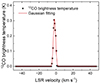 |
Fig. A.1. Spectrum of the 12CO brightness temperature of the MC proposed to be associated with J0007+5659u. The spectral data appears very smooth due to the application of moment masking. The red line shows the result of Gaussian fitting. |
Appendix B: Corner plots associated with MCMC fittings
For a fitting based on the MCMC method, it is conventional to use the corner plot showing the posterior PDF of each fitting parameter to reflect the convergence of the fitting and the correlation within parameters. If the MCMC fitting has reached convergence and the joint distribution function between parameters satisfies the normal distribution, the 2-D scatter diagram in the corner plot is supposed to exhibit a stable shape, approximately a circle or ellipse.
In Figs. B.1 and B.2, we present the corner plots associated with the MCMC fittings in our leptonic and hadronic modeling research. As shown by these figures, all the fitting are converged, while the distributions of some parameters seem to be more complicated than the expectations, due to the scarcity of constraints from experimental data. For our modeling research, there is still some room to improve by exploring better-suited fitting parameters in the models and obtaining more observational data in other energy bands.
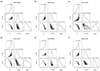 |
Fig. B.1. Corner plots showing the posterior PDF of αe, Ec, and d for the leptonic modeling research. Panels (a)-(f) present the results of J0007+5659u, J0206+4302u, J0212+4254u, J0216+4237u, J1740+0948u, and J1959+1129u, respectively. |
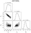 |
Fig. B.2. Corner plot showing the posterior PDF of Γ1, Γ2, and αp for the hadronic modeling research on J0007+5659u. |
Appendix C: Expected neutrino flux calculation
The production rate and spectrum of neutrinos from p-p interaction depend on the type of meson decay and the flavor of generated neutrinos. For muonic neutrinos, the neutrino flux per unit energy can be calculated via the equation below (Kelner et al. 2006; De Sarkar & Gupta 2022)
 (C.1)
(C.1)
where x = Eν/Ep is the variable of integration,  stands for the mean particle number density of 10.50 ± 3.08 cm−3 as presented in Sect. 2.4, Eν denotes the energy of produced neutrino, σpp(Eν/x) is the total inelastic cross section in p-p interaction as presented by Eq. (5), Jp(Eν/x) represents the energy distribution of protons as shown in Eq. (4), and Fν(x, Eν/x) describes the energy spectra of neutrinos produced through meson decay. For muonic neutrinos generated from the decays of charged pions and secondary muons respectively, Fν(x, Eν/x) have different forms (Kelner et al. 2006). The lower and upper limits of integration are also determined by the type of meson decay. In the pion decay scenario, since the Fν(x, Eν/x) has a sharp cutoff at x = 0.427 (Kelner et al. 2006), the upper limit of integration can be simply set at 0.427. Meanwhile, in the muon decay scenario, the integration should be performed with x varying from 0 to 1.
Based on Eqs. (4), (5), and (C.1), we calculated the expected muonic neutrino flux from J0007+5659u with the best-fit parameters in our hadronic model as presented in Sect. 3.2 of the main text and compared with the ten years of observation sensitivity of IceCube-Gen2 (Grant et al. 2019). Figure C.1 shows the result. The fluxes of other flavor neutrinos are expected to be the same as that of muonic neutrinos, as νe : νμ : νtau = 1 : 1 : 1 at Earth. As shown in Fig. C.1, the calculated neutrino SED of J0007+5659u is significantly lower than the sensitivity limit of IceCube-Gen2 with energy ranging from 1 TeV to 1 PeV.
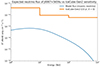 |
Fig. C.1. Expected muonic neutrino flux of J0007+5659u generated by p-p interaction, comparing with the ten years of observation sensitivity of IceCube-Gen2 (Grant et al. 2019). |
Moreover, the neutrino fluxes from γ-p interaction (Hümmer et al. 2010) for the six LHAASO UHE sources were also considered. We studied the interactions between the γ-photons emitted from the six sources and Galactic CR protons. Due to the weak γ-ray flux intensities of the six sources, the expected neutrino fluxes in γ-p interaction calculated with the Galactic CR proton spectrum (An et al. 2019) are much lower than those in p-p interaction.
All Tables
Overview of the six UHE γ-ray sources detected solely by LHAASO-KM2A (Cao et al. 2024), which are the focus of this study.
All Figures
|
Fig. 1. Fermi TS maps within the 5° radius ROIs around the six LHAASO UHE sources. Panels (a)–(d) show TS maps where the nearby 4FGL sources associated with the LHAASO sources are retained. Yellow dashed circles with a radius of 0 |
| In the text | |
|
Fig. 2. Planck all-sky map at 857 GHz. The map is presented in Galactic coordinates, and the color bar is plotted in logarithmic scale. The zoomed-in views of 10° × 10° ROIs centered on the six sources are presented at the top of the figure. The yellow dashed circles indicate the positions of labeled sources. |
| In the text | |
|
Fig. 3. Results of 12CO survey around the six LHAASO UHE sources. The data in panel (a) was integrated with a LSR velocity coverage from –4.9 km s−1 to 1.6 km s−1, covering the MC in proximity to J0007+5659u. For the data in panels (b)–(d), the LSR velocity integrating range was ±47.1 km s−1, reaching the limitation of this survey (Dame & Thaddeus 2022). The positions of the six LHAASO sources are marked by yellow dashed circles with radius of 0 |
| In the text | |
|
Fig. 4. Results of leptonic modeling research. Panel (a) shows the result of J0007+5659u. The solid blue line represents the total SED of γ-ray generated by leptonic interactions. The dashed and dotted lines in different colors are the SEDs contributed from synchrotron radiation, IC scattering, and bremsstrahlung. The pointing down arrows stand for the upper limits obtained from the observations of Swift-XRT, Fermi-LAT, and WCDA. The expected sensitivity of 3 × 10⁴ seconds’ observation with EPIC-pn of XMM-Newton has been shown by the thick golden line. The fitting SED of KM2A data with error bar is displayed by a butterfly plot filled in gray. Panels (b)–(f) are the results of J0206+4302u, J0212+4254u, J0216+4237u, J1740+0948u, and J1959+1129u, respectively. |
| In the text | |
|
Fig. 5. Best-fit result of the hadronic model for J0007+5659u, fit to the multiwavelength upper limits, compared with the best-fit result of the leptonic model. The solid blue line represents the SED of γ-ray generated by p–p interaction. The dashed line in red stands for the total SED of γ-ray generated by leptonic interactions. The pointing down arrows denote the upper limits of SED according to the observations of Swift-XRT, Fermi-LAT, and WCDA. Also, the expected sensitivity of 3 × 10⁴ seconds’ observation with EPIC-pn of XMM-Newton has been shown by the thick golden line. The fitting SED of KM2A data with error bar is displayed by a butterfly plot filled in gray. |
| In the text | |
|
Fig. 6. Results of γ-ray flux intensity map at 50 TeV generated for different values of D0. Panels (a)–(d) give the results for D0 = 4.8 × 1024 cm2 s−1, 1.2 × 1025 cm2 s−1, 2.8 × 1025 cm2 s−1, and 6.9 × 1025 cm2 s−1, respectively. For comparing with the physical image shown in the LHAASO catalog, the coordinate system used here is the J2000 equatorial frame. The other parameters adopted in the calculation are d = 0.4 kpc and v = 1600 km s−1. The white arrow indicates the proper motion direction of the pulsar, while the green star marks the current position of the pulsar. |
| In the text | |
|
Fig. 7. Results of γ-ray flux intensity map at 50 TeV generated for different values of d. Panels (a)–(d) give the results for d = 0.2 kpc, 0.4 kpc, 0.6 kpc, and 0.8 kpc, respectively. The other parameters adopted in the calculation are D0 = 4.8 × 1024 cm2 s−1 and v = 1600 km s−1. |
| In the text | |
|
Fig. 8. Results of γ-ray flux intensity map at 50 TeV generated for different values of v. Panels (a)–(d) give the results for v = 400 km s−1, 800 km s−1, 1200 km s−1, and 1600 km s−1, respectively. The other parameters adopted in the calculation are D0 = 4.8 × 1024 cm2 s−1 and d = 0.4 kpc. |
| In the text | |
|
Fig. 9. Predicted γ-photon count maps and smoothed significance maps for energies exceeding 25 TeV in the single traveling PWN modeling attempt. Panel (a) shows the γ-photon count map calculated with D0 = 4.8 × 1024 cm2 s−1, d = 0.4 kpc, and v = 1600 km s−1. The blue arrow indicates the proper motion direction of the hypothetical pulsar proposed in our model. Panel (b) shows the predicted significance map seen from LHAASO. The result has been smoothed with the LHAASO PSF at energies above 25 TeV (1 |
| In the text | |
|
Fig. 10. Predicted γ-photon count maps and smoothed significance maps for energies exceeding 25 TeV in the multiple traveling PWNe modeling attempt. Panels (a)–(b) show the γ-photon count map and significance map calculated with the model including PSR J0218+4232 and a hypothetical pulsar. The blue arrow indicates the proper motion direction of the hypothetical pulsar. Panels (c)–(d) show the γ-photon count map and significance map calculated with the model including two hypothetical pulsars. Here, the γ-ray emission from PSR J0218+4232 has been excluded. |
| In the text | |
|
Fig. A.1. Spectrum of the 12CO brightness temperature of the MC proposed to be associated with J0007+5659u. The spectral data appears very smooth due to the application of moment masking. The red line shows the result of Gaussian fitting. |
| In the text | |
|
Fig. B.1. Corner plots showing the posterior PDF of αe, Ec, and d for the leptonic modeling research. Panels (a)-(f) present the results of J0007+5659u, J0206+4302u, J0212+4254u, J0216+4237u, J1740+0948u, and J1959+1129u, respectively. |
| In the text | |
|
Fig. B.2. Corner plot showing the posterior PDF of Γ1, Γ2, and αp for the hadronic modeling research on J0007+5659u. |
| In the text | |
|
Fig. C.1. Expected muonic neutrino flux of J0007+5659u generated by p-p interaction, comparing with the ten years of observation sensitivity of IceCube-Gen2 (Grant et al. 2019). |
| In the text | |
Current usage metrics show cumulative count of Article Views (full-text article views including HTML views, PDF and ePub downloads, according to the available data) and Abstracts Views on Vision4Press platform.
Data correspond to usage on the plateform after 2015. The current usage metrics is available 48-96 hours after online publication and is updated daily on week days.
Initial download of the metrics may take a while.