| Issue |
A&A
Volume 698, June 2025
|
|
|---|---|---|
| Article Number | A322 | |
| Number of page(s) | 16 | |
| Section | Stellar atmospheres | |
| DOI | https://doi.org/10.1051/0004-6361/202452365 | |
| Published online | 26 June 2025 | |
Directly deriving atmospheric parameters for one million stars from SMSS photometric images
1
School of Mathematics and Statistics, Shandong University,
Weihai
264209,
Shandong,
PR China
2
School of Mechanical, Electrical and Information Engineering, Shandong University,
Weihai
264209,
Shandong,
PR China
★ Corresponding author: This email address is being protected from spambots. You need JavaScript enabled to view it.
Received:
25
September
2024
Accepted:
28
April
2025
Abstract
The precise determination of stellar atmospheric parameters (effective temperature Teff, surface gravity log g, and metallicity [Fe/H]) serves as a cornerstone of Galactic studies. In this work, we develop a novel deep learning approach, the Atmospheric CSWin Framework (ACF), to measure these parameters with high precision. The ACF employs a dual-input architecture that combines astrometric data (parallaxes and their corresponding errors) from Gaia Early Data Release 3 with photometric images from the fourth data release (DR4) of the SkyMapper Southern Survey (SMSS). The framework utilizes a CSWin Transformer backbone for hierarchical feature extraction from photometric images, integrated with Monte Carlo dropout in the prediction module for robust uncertainty quantification. Trained on cross-matched stars between SMSS DR4 and the third data release of the Galactic Archaeology with HERMES spectroscopic survey, the ACF achieves parameter estimates with dispersions of 95.02 K for Teff, 0.07 dex for log g, and 0.14 dex for [Fe/H]. Systematic experiments demonstrate that incorporating parallax information significantly improves the precision of all three parameters, especially log g. Our image-based methods outperform traditional approaches based on stellar magnitudes or colors, with improvements ranging from 2% to 14%. The ACF yields parameter estimates approaching those of high-resolution spectroscopic analyses, and the framework remains effective even for low-quality samples, highlighting its robustness and general applicability. Using the ACF, we compiled a comprehensive catalog of atmospheric parameters for one million SMSS DR4 stars.
Key words: methods: data analysis / methods: statistical / techniques: photometric / stars: abundances / stars: fundamental parameters
© The Authors 2025
 Open Access article, published by EDP Sciences, under the terms of the Creative Commons Attribution License (https://creativecommons.org/licenses/by/4.0), which permits unrestricted use, distribution, and reproduction in any medium, provided the original work is properly cited.
This article is published in open access under the Subscribe to Open model. This email address is being protected from spambots. You need JavaScript enabled to view it. to support open access publication.
1 Introduction
In astrophysics, precise measurements of stellar atmospheric parameters-effective temperature (Teff), surface gravity (log g), and metallicity ([Fe/H])-are fundamental to understanding the formation and chemical evolution of the Milky Way. These parameters serve as critical tracers of stellar populations, enabling the reconstruction of the Galaxy’s assembly history and dynamical processes (Robin et al. 2003; Matteucci 2021).
Over the past few decades, the advent of large-scale spectroscopic surveys has revolutionized our ability to study stellar atmospheric parameters. Surveys such as the Large Area MultiObject Fiber Spectroscopic Telescope (LAMOST; Deng et al. 2012; Liu et al. 2014), Galactic Archaeology with HERMES (GALAH; De Silva et al. 2015), the Apache Point Observatory Galactic Evolution Experiment (APOGEE; Majewski et al. 2017), the Radial Velocity Experiment (RAVE; Steinmetz et al. 2006), the Sloan Extension for Galactic Understanding and Exploration (SEGUE; Yanny et al. 2009; Rockosi et al. 2022), and the Gaia-ESO Public Spectroscopic Survey (Gilmore et al. 2022; Randich et al. 2022) have provided extensive spectroscopic data. Concurrently, astronomers have developed advanced methods for estimating atmospheric parameters from spectroscopic data (Bu & Pan 2015; Soubiran et al. 2022; Tabernero et al. 2022; Yang et al. 2023). However, despite the high precision of spectroscopic analyses achieved through efficient pipelines, certain challenges persist in specific regimes. For example, observations of extremely faint or distant stars, or those that require specialized wavelength coverage or high spectral resolution, still face trade-offs between observational cost, target selection feasibility, and computational efficiency (Ivezic et al. 2008; Huang et al. 2019).
In contrast, photometric surveys offer a more efficient and cost-effective alternative (Casagrande et al. 2019; Yang et al. 2022). These surveys use sensitive optical detectors and customized filters to enable rapid and comprehensive data collection, making them ideal for large-scale studies. A prominent example is the Sloan Digital Sky Survey (SDSS; York et al. 2000), which, through expansive optical observations encompassing nearly the entire Northern Hemisphere, provides comprehensive brightness and color information for billions of celestial objects. Other large-scale photometric surveys include the Two Micron All Sky Survey (2MASS; Skrutskie et al. 2006), the Wide-field Infrared Survey Explorer (WISE; Wright et al. 2010), the Pan-STARRS1 survey (PS1; Chambers et al. 2016), the Gaia mission (Gaia Collaboration 2016, 2018), the SkyMapper Southern Survey (SMSS; Wolf et al. 2018), and the Stellar Abundance and Galactic Evolution Survey (SAGE; Zheng et al. 2018), all of which provide vast amounts of photometric data, making significant contributions to Galactic research.
Numerous studies have focused on deriving atmospheric parameters from magnitudes or colors obtained from photometric data. For instance, Yuan et al. (2015) estimates photometric metallicity by fitting dereddened colors obtained from the SDSS. Huang et al. (2019) employs polynomial regression to establish relationships between the atmospheric parameters of red giants and photometric colors from SMSS. Additionally, Casagrande et al. (2019) identifies correlations between stellar metallicities and specific photometric magnitudes (v and g from SMSS, as well as KS from 2MASS). Furthermore, Kim & Lépine (2022) developed an empirical color-magnitude-metallicity grid, which is particularly advantageous for estimating photometric metal-licities in low-mass, metal-poor stars. Despite their widespread adoption, these photometric methods face limitations due to their reliance on magnitude system transformations, which typically discard spatial information inherent in raw photometric imagesinformation that could further refine atmospheric parameter estimation. Moreover, the measurement of stellar magnitudes is prone to systematic biases induced by aperture effects or filterdependent calibration errors (Wolf et al. 2018; Onken et al. 2019), which can undermine the precision of derived atmospheric parameters.
The emergence of deep learning has opened new avenues for overcoming these limitations and enables direct analysis of photometric images. Unlike traditional indirect parameters, such as magnitudes or colors, photometric images preserve complete observational information. Although, in theory, the intensity profile of a single star can be perfectly described as a point source convolved with the point spread function (PSF), and the derived PSF photometry provides near-perfect characterization of stellar flux, using raw images rather than derived measurements does not automatically enhance parameter estimation precision. However, under real, nonideal observing conditions, derived photometric measurements are susceptible to contamination from adjacent stars, whereas deep learning-based modeling approaches that utilize original image data effectively mitigate such interference. Furthermore, for large-scale sky surveys, even marginal improvements in individual stellar measurements, when aggregated across tens of thousands of stellar samples, substantially enhance the statistical reliability of the results.
In recent years, numerous successful astronomical studies have directly utilized imaging data, demonstrating remarkable achievements in extracting astrophysical signals from raw pixellevel observations. For example, He et al. (2021) built a source detection system that uses deep learning to identify and categorize astronomical sources within image data as quasars, stars, or galaxies. Arcelin et al. (2021) developed a novel galaxy deblending method using variational autoencoders that learn probabilistic models directly from multiband observational data, achieving significant improvements in ellipticity and magnitude reconstruction accuracy. Additionally, Dey et al. (2022) introduced a novel deep capsule network that discerns morphological characteristics from SDSS photometric images to estimate photometric redshifts. These studies demonstrate remarkable success in extracting astrophysical signals directly from imaging data. Building on previous exploratory research, Wu et al. (2023) pioneered the application of Bayesian neural networks (BNNs) to estimate stellar atmospheric parameters from photometric images, achieving promising results. However, due to the inherent limitations of SDSS images, which are susceptible to saturation effects, their research was restricted to approximately 3000 Northern Hemisphere stars, reducing the universality and representativeness of the findings. In addition, their uncertainty estimates rely on simplified variance assumptions, which underestimated the true predictive errors. These limitations underscore the need for a robust, scalable framework capable of leveraging modern, large-scale photometric surveys while rigorously quantifying uncertainties.
In this work, we address these critical gaps by proposing the Atmospheric CSWin Framework (ACF), an innovative deep learning architecture that combines the CSWin Transformer for enhanced image feature extraction with Monte Carlo (MC) dropout for reliable uncertainty quantification. We assembled combined training and validation sets of 106 145 high-quality stars from the Southern Hemisphere, more than 30 times the size of the previous image-based atmospheric parameter study (Wu et al. 2023), ensuring robust statistical significance and improved generalization capabilities. Through extensive comparative experiments, we demonstrate marginal but consistent improvements in image-driven methods compared to traditional magnitude- or color-based approaches. Finally, leveraging the ACF, we compile a catalog of precise atmospheric parameters for one million Southern Hemisphere stars, providing a valuable new resource for investigating the formation and chemical evolution of the Milky Way.
The paper is organized as follows. In Sect. 2, we describe the photometric samples used in this work, along with the methods used for sample selection and processing. In Sect. 3, we introduce the proposed ACF with its two main components, the CSWin Transformer and MC dropout, and provide implementation details for training models. Section 4 presents the experimental results, including the precision and uncertainty of the regression for the three stellar atmospheric parameters. In Sect. 5, we conduct a set of comparative experiments that validate the robustness of our parameter estimations based on photometric images. We describe the final catalog of atmospheric parameters for one million stars in Sect. 6. Finally, we present a brief conclusion in Sect. 7.
2 Data
2.1 Data description
In this study, we used photometric images from the fourth data release (DR4) of SMSS (Onken et al. 2024). The SMSS is a deep, optical, wide-field astronomical survey that focuses on imaging the entire Southern Hemisphere. This survey is designed to achieve a depth of 20-22 magnitudes in six optical bands (u, v, g, r, i, and z). The SkyMapper photometric system strategically divides the SDSS u band into two optimized bands: A violet-sensitive v band, analogous to the DDO 38 filter (McClure 1976) which covers the Ca II doublet (Ca H at 3933.7 Å and Ca K at 3968.5 Å) and provides exceptional metallicity sensitivity; and an ultraviolet-enhanced u band similar to the Stromgren photometric system (Stromgren 1951), which covers the Balmer discontinuity and provides good temperature sensitivity in hot stars, as well as gravity sensitivity for AFG-type stars (Bessell 2005). The survey uses a 1.35-meter telescope located at the Siding Spring Observatory in Australia, equipped with a mosaic composed of thirty-two 2k 4k CCD detectors. The SMSS DR4, released in February 2024, contains more than 400 000 images that cover 26 000 deg2 of the sky and catalogs more than 700 million unique astrophysical objects. These catalogs1 include a photometry table with one row per detection and a master table with one row per unique astrophysical object, combining multiple detections. All photometric images were initially processed and calibrated with the Science Data Pipeline (Luvaul et al. 2017; Wolf et al. 2017) and selected using several quality control criteria (Onken et al. 2024).
We used stellar atmospheric parameters from the third data release of the GALAH survey, specifically GALAH+ DR3 (Buder et al. 2021). The GALAH survey, utilizing the HERMES spectrograph on the 3.9-meter Anglo-Australian Telescope, is designed to acquire spectra for approximately one million stars to facilitate Galactic archaeology. It captures optical spectra across four non-contiguous wavelength channels (4713-4903 Å, 56485873 Å, 6478-6737 Å, and 7585-7887 Å), with a resolution of R ~ 28 000. The GALAH+ DR3 significantly expanded the survey to include 678 423 stellar spectra. These observations, which were conducted between November 2013 and February 2019, mainly focus on 588 571 stars. Stellar parameters (extracted from the GALAH_DR3_main_allstar_v2.fits catalog2) were derived using an improved analysis approach known as Spectroscopy Made Easy (Valenti & Piskunov 1996; Piskunov & Valenti 2017). This advancement relies on absorption features with reliable line information for spectrum synthesis, enhancing the continuity and precision of stellar parameters.
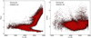 |
Fig. 1 Distribution of samples in the Teff−log g plane (left) and the Teff−[Fe/H] plane (right). Black and red dots represent the training and validation sets, respectively, with a ratio of 8:2. |
2.2 Data selection
To obtain the spectroscopic atmospheric parameters (Teff, log g, and [Fe/H]) corresponding to the photometric images, we first cross-matched the SMSS DR4 master table with the GALAH+ DR3 catalog. After excluding stars with missing atmospheric parameters, a total of 555 323 common stars remained. Specifically, photometric images provide the most direct information about stars. However, they are often compromised by noise interference, such as cosmic rays and other nearby sources, which can degrade image quality and subsequently affect algorithm performance. Therefore, to obtain reliable photometric estimates, we applied a set of criteria to select high-quality samples. First, to minimize interstellar extinction, we required that stars have a Galactic latitude |b| ⩾ 10. Second, we selected stars with reliable spectroscopic parameters from GALAH+ DR3: flag_sp = 0, flag_fe_h = 0, and snr_c3_iraf > 30. Third, we retained only those with good quality photometric images from SMSS DR4: flags = 0 and class_star ⩾ 0.6. We also required that each star have at least one valid detection in any DR4 SMSS filter, such that {f}_ngood ⩾ 1, where f is the filter name. In addition, we excluded targets containing other sources within a distance of 15 arcseconds in a photometric image: self_dist1 = 15. Finally, all stars had reliable parallax measurements from Gaia Early Data Release 3 (Gaia EDR3) with uncertainties smaller than 30%.
After applying the above criteria, we obtained 106 145 stars. We then cross-matched these stars with the SMSS DR4 photometry table to obtain multiple detections for each object and each filter. To ensure consistency with the magnitudes provided by the SMSS DR4 master table, we retained only detections that satisfied use_in_clipped = 1. All photometric data were stored in Flexible Image Transport System (FITS) files (Pence et al. 2010). We then downloaded them according to the parameters “ra, dec, image_id, and ccd” of each detection. We note that full CCD images were not downloaded, as they would contain many other field stars. As in Wu et al. (2023), we fixed the download size to 48 × 48 pixel2. Finally, we randomly divided the 106 145 stars into training and validation using an 8:2 ratio. Both sets exhibit a consistent distribution, as shown in Fig. 1. The Teff of these samples ranges from 4000 K to 8000 K, the log g spans from 0 to 5, and the [Fe/H] varies between −3 and +1.
2.3 Data processing
Due to various factors, such as atmospheric conditions and exposure duration, significant differences can exist between different photometric images of the same filter for each object (see Fig. 2). To eliminate these differences, we first subtracted the sky level from the background using the photometry table. Next, we corrected the fluxes within the photometric images by applying the zeropoint derived from the photometry table. In addition, we corrected for interstellar reddening using maps from Schlegel et al. (1998), with bandpass absorption coefficients provided on the official SMSS website3. The “Corrected” panel in Fig. 2 displays the calibrated photometric images, showing consistent flux distributions across all detections within each corresponding band.
Next, we aligned the photometric images across different bands using Python’s REPROJECTION4 toolkit as in He et al. (2021). This alignment was necessary because the CCDs captured images at different times, leading to slight positional deviations. By referencing one of the r-band images for each object and utilizing the World Coordinate System in the FITS headers, we ensured that all photometric images in the six bands (u, v, g, r, i, and z) were precisely aligned for consistent astronomical analysis.
Each object can have multiple detections within a given filter. To generate composite images, we adopted a straightforward averaging method, in which each detection contributes equally to the final stacked image, as described by the following equation:
 (1)
(1)
where n represents the total number of detections for the band, Ii denotes the photometric image of the i-th detection, and Istacking is the resulting stacked image. This stacking method ensured a more comprehensive and representative composite image for each band. As a result, each object is represented by six meticulously stacked images (see the “Stacked” panel in Fig. 2).
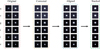 |
Fig. 2 Visualization of the data processing procedure. The “Original” panel displays the raw photometric images of a target object across six bands (u, v, g, r, i, and z) from the SMSS DR4, where each band can include multiple detections. For clarity, only two representative detections are shown. The “Corrected” panel shows the photometric images after applying zeropoint and reddening corrections. Subsequently, image reprojection is performed to achieve precise spatial alignment, as demonstrated in the “Aligned” panel. Finally, the “Stacked” panel presents the stacked photometric images generated through a simple averaging method. |
3 Methods
3.1 CSWin Transformer
The CSWin Transformer (Dong et al. 2022) is an advanced vision transformer architecture designed to improve efficiency and performance in image processing tasks. Its novel crossshaped window self-attention mechanism captures information from both horizontal and vertical directions. This approach was particularly well suited for processing point-spread star images in this study.
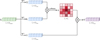 |
Fig. 3 Illustration of the standard self-attention mechanism. The input matrix X of size L Demb is transformed into the query (Q), key (K), and value (V) matrices, each of size L Dout, through weight matrices WQ, WK, and WV. The attention matrix A is computed by taking the dot product of Q and K, followed by a softmax operation. The final output Y of size L Dout is obtained by multiplying A with V. |
3.1.1 Standard self-attention
The standard self-attention (SA) mechanism (Vaswani et al. 2017) computes relationships between all elements within a sequence to capture global dependences (see Fig. 3). Given an embedded input  , where L is the sequence length and Demb is the embedding dimension, we obtain the query (Q), key (K), and value (V) by applying linear projections to X with Q = XWQ, K = XWK, and V = XWV. Here,
  ,
,  , and
, and  are parameter matrices, and Dout is the projection dimension. The similarity between Qi and Kj is calculated to obtain the attention matrix, which is expressed as:
 (2)
(2)
where ![Mathematical equation: $(softmax[X])_{ij} = \exp{X_{ij}}/\sum_{k}\exp{X_{ik}}$](/articles/aa/full_html/2025/06/aa52365-24/aa52365-24-eq7.png) .
.
With the attention matrix, the SA mechanism allows the model to focus on different parts of the sequence by weighting input features differently:
 (3)
(3)
The multi-head self-attention (MHSA) mechanism is an extension of SA that enables the model to focus on information in different representation subspaces in parallel. In MHSA, each head independently generates its own Q, K, and V matrices, leading to unique attention computations. Integrating multiple attention matrices yields the output of the MHSA:
 (4)
where
(4)
where  , Nh is the number of heads, and Dh = Demb/Nh is the embedding dimension of each head. The S Ah(X) of the h-th head follows Eq. (3).
3.1.2 Cross-shaped window self-attention
The cross-shaped window self-attention (CSWin-Attention) mechanism is the key module in the CSWin Transformer. Unlike traditional SA mechanisms that rely on global attention, CSWin-Attention computes attention weights along both horizontal and vertical axes simultaneously. This design significantly reduces the computational complexity of SA, which typically scales quadratically with input size, while maintaining the ability to capture both local and global dependencies.
We let  represent the input feature map, where H and W are height and width, and C is the number of channels. This feature map was first linearly projected to K heads, which were split into two groups: Group A and Group B (see Fig. 4). Each group contained K/2 heads. Group A was used to calculate horizontal self-attention, while Group B was used for vertical self-attention.
Taking horizontal self-attention as an example, Group A was segmented into nonoverlapping horizontal stripes, denoted as [X1, X2,..., XM], each with equal width sw, where M = H/sw and sw is a hyperparameter representing the stripe width. Each horizontal stripe contains sw W tokens.  ,
,  , and
, and  are queries, keys, and values for the i-th horizontal stripe Xi of the k-th head. We have
  ,
,  , and
, and  , where
  ,
,  , and
, and  are parameter matrices, and dk = C/K. The self-attention for horizontal stripes Xi of the k-th head was defined as
 (5)
(5)
By concatenating the self-attention of M horizontal stripes, we obtained the overall horizontal stripe self-attentions for k-th head, which was defined as
![Mathematical equation: \mathrm{H\text{-}Attention}_k(X) = [Y^1_k, Y^2_k, \dots, Y^M_k].](/articles/aa/full_html/2025/06/aa52365-24/aa52365-24-eq22.png) (6)
(6)
Similarly, Group B was segmented into nonoverlapping vertical stripes with equal width xw along the horizontal direction. The overall vertical stripes self-attention for the k-th head was denoted as V-Attentionk(X). Both groups computed horizontal and vertical stripe self-attentions in parallel. The outputs were then concatenated to obtain the CSWin-Attention, defined as
 (7)
(7)
where  is a learnable projection matrix. By combining horizontal and vertical self-attention, the CSWin Transformer captured long-range dependencies across both spatial dimensions while reducing computational cost compared to global self-attention.
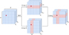 |
Fig. 4 Illustration of the cross-shaped window self-attention. A feature map of shape H W C is first linearly projected to K heads. This is then split into Group A and Group B to calculate horizontal and vertical self-attention in parallel. Finally, the outputs of the two groups are concatenated to obtain the cross-shaped window self-attention. |
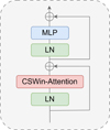 |
Fig. 5 Structure of the CSWin Transformer block. The CSWin-Attention refers to cross-shaped window self-attention, which is detailed in Sect. 3.1.2. |
3.1.3 CSWin Transformer block
The CSWin Transformer block is the fundamental building unit of the CSWin Transformer architecture. Its overall structure follows a standard transformer block design but leverages the CSWin-Attention mechanism to efficiently capture local and global dependencies in images (see Fig. 5). It is defined as
 (8)
(8)
where Xl represents the output of l-th CSWin Transformer block or the preceding convolutional layer of each stage, LN denotes layer normalization, and MLP represents multi-layer perceptron layers. Each sublayer (CSWin-Attention and MLP) was first processed by LN and then followed by residual connections to stabilize the training process and improve gradient flow. After the attention operation, the output  was passed through a standard two-layer MLP with a nonlinear activation function between the layers.
3.1.4 CSWin Transformer architecture
Figure 7 (bottom panel) illustrates the architecture of the CSWin Transformer used in this work. We first split the input photometric image of shape 48 × 48 × 6 into overlapping patches using a patch embedding layer with a convolution of kernel size 7 × 7 and stride 2. This design ensured that local features were preserved while reducing the spatial resolution, yielding patch tokens with a shape of 24 × 24. We set the embedding dimension of each token to 64 to balance computational efficiency and feature representation. These patch tokens were then fed into a hierarchical architecture consisting of four stages. Each stage contained multiple CSWin Transformer blocks (N = [2, 4, 32, 2]), where CSWin-Attention was applied with dynamically increasing stripe width (sw = [1, 2, 3, 3]) across stages. This progressive increase in stripe width allowed the model to capture both local and global dependencies effectively. The number of channels started at 64 in the first stage and doubled at each subsequent stage (i.e., 128, 256, 512), enabling the network to learn increasingly complex features. Between two adjacent stages, downsampling was performed using a convolution with a kernel size of 3 × 3 and stride 2. This reduced the spatial resolution by half while doubling the channel dimension, ensuring a balance between computational efficiency and feature richness. After the final stage, the feature map was reduced from the original shape of 48 × 48 × 6 to 3 × 3 × 512. It was then passed through an LN layer and a global average pooling (GAP) layer, resulting in a feature map of size 1 × 1 × 512. This was flattened to a 512-dimensional feature vector and fed into subsequent MLP layers for atmospheric parameter regression.
3.2 Monte Carlo dropout
Uncertainty quantification is essential for deriving atmospheric parameters, as it provides a measure of the reliability of predictions. Traditional neural networks typically provide point estimates for parameters, treating model weights as fixed values. This approach fails to capture the uncertainty associated with model predictions. To address this issue, we employed MC dropout (Gal & Ghahramani 2016), an effective method for approximating the uncertainty inherent in BNNs (Buntine 1991; MacKay 1992).
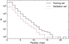 |
Fig. 6 Parallax distribution on a logarithmic scale for all samples. The black line and red dashed line represent the training and validation sets, respectively. |
3.2.1 Bayesian neural networks
Bayesian neural networks introduce a prior distribution over the model weights, treating them as random variables. This allows for uncertainty estimates in model predictions. Given a training dataset D, the objective was to compute the posterior distribution of the output y for a given input x*:
 (9)
(9)
where ω denotes the model weights of the BNNs, p(y*|x*,ω) represents the likelihood function, and p(ωD) is the posterior distribution of the weights. This implied that predicting the unknown output y* was equivalent to using an ensemble of an infinite number of neural networks with various weight configurations.
However, directly computing the posterior distribution p(ω|D) for BNNs was intractable in practice. Instead, variational inference (Graves 2011) is commonly used to approximate this distribution by minimizing the Kullback-Leibler (KL) divergence between the variational distribution q(ω) and the true posterior distribution p(ω|D):
 (10)
(10)
3.2.2 Monte Carlo dropout as an approximation of BNNs
The MC dropout simulates the behavior of BNNs by applying dropout during the test time. For a neural network with L layers, let Wi represent the weight matrix with dimensions Ki Ki - 1 of the i-th layer. Considering the variational distribution q(ω), each column of the weight matrix Wi was independently sampled from a Bernoulli distribution:
![Mathematical equation: W_i = M_i \cdot \text{diag}([z_{i,j}]_{j=1}^{K_i}),](/articles/aa/full_html/2025/06/aa52365-24/aa52365-24-eq29.png) (11)
(11)
where zi,j ~ Bernoulli(pi) for i = 1,..., L, j = 1,..., Ki - 1, pi is the dropout probability, and Mi is the matrix of variational parameters. When zi,j = 0, the corresponding unit j in layer i - 1 is removed as an input to layer i. This method enabled dropout to be maintained during test time, using different weight realizations for each forward pass. We therefore obtained an approximate predictive distribution:
 (12)
(12)
By employing MC sampling, we estimated the first moment of the predictive distribution:
 (13)
(13)
where T is the number of sampling times. In practice, this was equivalent to performing T random forward passes through the neural network and averaging the results as the final prediction. Similarly, the second moment was estimated as
 (14)
(14)
where  is the model’s precision hyperparameter, λ is the weight regularization term, l is the prior lengthscale factor, and ID is the identity matrix. Consequently, the predictive variance of the model was given by
 (15)
(15)
3.3 Overall framework
To address the inherent limitation of single photometric images in capturing stellar distance information-a critical factor for precise atmospheric parameter determination, as demonstrated in our comparative experiments in Sect. 5.1 - we cross-matched all samples with Gaia EDR3 (Gaia Collaboration 2021) to obtain parallax measurements, which served as a distance indicator (Cantat-Gaudin et al. 2020). Figure 6 shows that most stars have parallaxes within 5 milliarcseconds. However, the observed parallaxes contained non-negligible measurement errors (up to 30% for our samples, as detailed in Sect. 2.2). More critically, when parallax errors were significant, the naive reciprocal transformation yielded systematically biased distance estimates (Bailer-Jones 2015; Luri et al. 2018), which subsequently propagated into atmospheric parameter estimates. To minimize this systematic effect, we simultaneously incorporated both parallax measurements and their associated errors. Given that parallaxes and their errors are scalar quantities that cannot be directly concatenated with 2D photometric images for convolutional neural network processing, we designed a dual-input architecture, as illustrated in Fig. 7.
Specifically, the astrometric branch took parallaxes and their associated errors as input. A 128-dimensional fully connected layer then performed joint encoding of these astrometric parameters, projecting them into a high-dimensional distance-aware representation space. For the photometric branch, to comprehensively retain implicit information, we integrated the photometric images from all bands (u, v, g, r, i, and z), resulting in a six-channel input image with a shape of 48 × 48 × 6. This input image was first fed into the CSWin Transformer for feature extraction (detailed in Sect. 3.1.4), which produced a 512-dimensional visual feature representation. The two complementary representations were then concatenated to form a comprehensive 640-dimensional feature vector that spatially aligned photometric characteristics with geometric constraints. Building upon this fused representation, we constructed a prediction module to map it to the label space, comprising three fully connected layers with nonlinear activation functions. To effectively quantify prediction uncertainty, MC dropout was systematically applied throughout each layer. During both training and testing phases, neurons in each layer were randomly deactivated according to predetermined dropout rates. Consequently, the resulting output varied each time and followed a specific distribution. The final parameter estimate was derived by averaging multiple sampled outputs, with the variance providing an assessment of the prediction uncertainty.
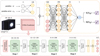 |
Fig. 7 Architecture of the Atmospheric CSWin Framework used for regression tasks. The framework employed a dual-input architecture to process both astrometric and photometric data. The astrometric branch (top left, gray frame) took parallaxes and their associated errors as input. These parameters were jointly encoded through a 128-dimensional fully connected layer. In parallel, the photometric branch (middle left, pink frame) processed six-band (u, v, g, r, i, and z) images with dimensions 48 × 48 × 6. These images were fed into a CSWin Transformer backbone network (bottom, pink frame), which performed hierarchical feature extraction across four progressive stages. Each stage contained multiple CSWin Transformer blocks, which captured both local and global spatial information through CSWin-Attention mechanism. Through this process, the backbone generated a 512-dimensional visual feature representation. The framework then combined these complementary representations through concatenation (denoted by ©) to form a 640-dimensional composite feature vector. This fused feature vector served as input to the prediction module (top right, orange frame), which consisted of three fully connected layers incorporating MC dropout. The expected value of multiple sampled outputs from the prediction module, denoted as E(Yh), served as the model’s prediction y* (i.e., Teff, log g, or [Fe/H]). The variance of these sampled outputs, denoted as D(Yh), was used to assess the uncertainty σ* of the model’s prediction. |
3.4 Implementation details
3.4.1 Training hyperparameters
All models were trained for 300 epochs with a batch size of 128 using NVIDIA GeForce RTX 4060 Ti GPU, which was chosen to balance computational efficiency and gradient stability during training. We used the Adam optimizer with β1 = 0.99 and β2 = 0.999, as these values were well suited to stabilizing the optimization process in deep learning tasks involving sparse gradients. The initial learning rate was set at 0.0001 and decayed by a factor of 0.8 every 50 epochs. This learning rate schedule was selected to ensure steady convergence while avoiding overshooting during optimization. To prevent overfitting, we applied L2 regularization with a coefficient of 0.00005. This value was chosen based on preliminary experiments to strike a balance between model complexity and generalization performance. Additionally, a dropout rate of 0.2 was employed during both the training and testing stages of the model. The model weights were initialized using a truncated normal distribution, which helped avoid extreme initial values that could hinder convergence.
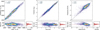 |
Fig. 8 Regression results for three stellar atmospheric parameters in the validation set: Teff (left panel), log g (middle panel), and [Fe/H] (right panel). The top part of each panel show spectroscopic labels versus photometric predictions derived using the algorithm described in Sect. 3. The lower-left part of each panel displays the residuals between photometric predictions and spectroscopic labels, with the overall offset (μ) and standard deviation (σ) indicated in the top-left corner of the top plot. To enhance clarity and visualize trends, kernel density estimation (KDE) is used to model the probability densities of the results, represented as a color gradient ranging from purple (low density) to red (high density). The lower-right part of each panel shows the probability density of the residuals fitted using KDE. Black dashed lines denote the one-to-one relationship, while red dashed lines mark zero residuals. |
3.4.2 Data augmentation
Photometric images were used to measure the luminosity of stars as well as their variability. Any artificially introduced changes, such as arbitrary brightness adjustments, could obscure genuine signal variations and consequently affect the analysis and understanding of these objects. Therefore, to ensure that the true physical information was preserved while enhancing model performance, we applied only data augmentation techniques such as random rotation and random flipping. These methods have also been shown to be effective in other studies (Dey et al. 2022; Wu et al. 2023).
3.4.3 Loss functions
The loss function chosen was the smooth L1 loss, a commonly used regression loss function in deep learning defined as
 (16)
(16)
where x represents the residual error between predictions and true values. For small errors (|x| < 1), smooth L1 loss behaved like the L2 loss, offering a quadratic penalty, which provided a higher sensitivity to small deviations. However, for larger errors, it transitioned to the L1 loss, which imposed a linear penalty and was less sensitive to outliers. This property makes smooth L1 loss particularly effective in scenarios where robustness to outliers is essential.
4 Results
This section presents the optimal experimental results for estimating stellar atmospheric parameters from SMSS DR4 photometric images. We provide a comprehensive analysis of the estimates, focusing on the precision of the regressions and their associated uncertainties.
4.1 Precision of regression
Figure 8 shows the regression results for three stellar atmospheric parameters in the validation set. For Teff, the photometric estimates exhibit a strong linear correlation with the spectroscopic labels along the black dashed one-to-one line. The kernel density estimation (KDE) heatmap reveals a dense concentration of data points along the diagonal (red to purple color gradient), indicating excellent agreement between model predictions and labels. Residual analysis shows only a slight systematic offset of −0.15 K with a dispersion of 95.02 K. The symmetric Gaussian distribution of the residual probability density, peaked near zero, further confirms the reliability of the predictions.
Our photometric log g results demonstrate remarkable consistency with high-resolution spectroscopic measurements in the range 1 < log g < 5, achieving a minimal dispersion of 0.07 dex. However, a systematic overestimation occurs at log g < 1, where the model predictions deviate from the spectroscopic labels. This discrepancy is partially attributable to the scarcity of training samples in this parameter space (see Fig. 1), but also reflects a known limitation of regression-based methods: the regression-toward-the-mean effect. As demonstrated in similar photometric studies (Ting 2024), models trained on imbalanced data tend to predict values closer to the mean of the training distribution when extrapolating to parameter extremes. While this bias does not significantly affect the bulk of our sample (log g > 1), it limits the reliability of log g estimates for low-gravity stars.
For [Fe/H], the photometric estimates agree well with the GALAH+ DR3 values in the metal-rich region ([Fe/H] > −1). However, a significant offset of +1 to +2 dex is observed in the metal-poor region ([Fe/H] ⩽ −1). This arises from the fact that the SMSS survey employs only two narrow and medium-band filters, specifically the u and v bands. Due to contamination from molecular carbon bands, the photometric estimate of [Fe/H] often results in systematic overestimation by 1 to 2 dex, particularly for very metal-poor stars (Huang et al. 2024). In addition, this regression effect further exacerbates the problem. Specifically, the model’s predictions cluster near the metallicity distribution peak of the training set ([Fe/H] 0.5), leading to systematic overestimation of [Fe/H] for extremely metal-poor stars. This highlights a critical trade-off in photometric metallicity estimation: although our method achieves high precision for [Fe/H] > -1, the combined effects of instrumental limitations and model bias preclude reliable metallicity gradient measurements in the metal-poor tail. To mitigate this, future work could incorporate spectroscopic priors for metal-poor stars.
The biases observed at the extremes of log g and [Fe/H] underscore a fundamental challenge in data-driven stellar parameter estimation. While our model achieves high precision within the densely sampled regions of the training data, extrapolation to the edges of parameter space introduces systematic uncertainties. These limitations are not unique to our approach; similar biases have been reported in other photometric and spectroscopic machine learning (ML) studies (Ness et al. 2015; Ting 2024).
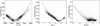 |
Fig. 9 Model uncertainties for three stellar atmospheric parameters: Teff (left panel), log g (middle panel), and [Fe/H] (right panel). Kernel density estimation (KDE) is used to approximate the probability density functions of model uncertainties. Areas of darker color represent regions of lower probability densities, while lighter areas indicate higher probability densities. The red solid lines show second-order polynomial regression curves, that delineate the trend between uncertainties and atmospheric parameters. The red shaded area corresponds to the 95% confidence interval of the regression. Its width represents the size of confidence interval and the variation reflects changes in predictive uncertainty as a function of atmospheric parameters. |
4.2 Uncertainty of regression
Figure 9 presents a detailed characterization of the prediction uncertainties of three stellar atmospheric parameters through KDE analysis. For effective temperature, the KDE heatmap reveals a characteristic U-shaped uncertainty distribution. The minimum uncertainty (lightest color region) is concentrated around the median temperature range (near 5500 K), where samples are most abundant. As temperatures deviate toward both extremes, uncertainties increase exponentially, rising sharply from 23 K at 5500 K to 258 K above 8000 K (an 11-fold increase). The uncertainty distribution of surface gravity exhibits significant asymmetry: while the high-gravity regime (log g > 3) maintains stable uncertainties of <0.1 dex, the low-gravity regime (log g < 2) exhibits a notable increase to ~0.22 dex. This pattern directly correlates with the sparsity of training samples in this parameter space, as visualized by the gradual color gradient in the KDE map. Metallicity predictions reveal a striking dichotomy: metal-rich stars achieve a low uncertainty of 0.03 dex, whereas the metal-poor regime shows a sharp rise in uncertainty, reaching 0.4 dex (a 13-fold increase). Notably, as metallicity decreases, the 95% confidence interval monotonically expands, reflecting both the exponentially declining abundance of metal-poor samples and systematic measurement biases introduced by molecular carbon bands (Huang et al. 2024).
5 Validation
5.1 Comparison with parallax-free framework
To systematically evaluate the contribution of parallax information to stellar atmospheric parameter estimation, we designed a comparative framework based solely on photometric images, termed the Atmospheric CSWin Parallax-free Framework (ACPF). This framework adopts a single-input architecture, with the first fully connected layer in the prediction module adjusted to 512 neurons (compared to 640 neurons in the dual-input ACF framework). All other components, including the CSWin Transformer backbone and MC dropout module, remain identical to those in ACF. The experiments use the same dataset and training strategy detailed in Sect. 3.4 to ensure rigorous comparison.
Figure 10 presents the predictions of ACPF for the three stellar atmospheric parameters. For Teff and [Fe/H], the photometric predictions show good agreement with the spectroscopic labels in the primary distribution range (aligned along the black dashed lines). Residual analysis reveals that while the systematic offsets remain near zero, the dispersion increases significantly (about 11%) compared to the ACF predictions in Fig. 8, indicating a noticeable decline in precision. The KDE curves confirm that residuals are concentrated near zero, suggesting that most predictions remain acceptable despite the lack of parallax constraints.
However, the parallax-free framework exhibits clear difficulties in predicting log g. When log g > 4, the data points display an anomalous rectangular distribution pattern, implying partial confusion between dwarfs and red clump stars in the absence of parallax constraints. Similar phenomena have been observed in other works (Liang et al. 2022; Wu et al. 2023; Khalatyan et al. 2024). Upon introducing parallax constraints, the precision of log g prediction improves dramatically-the dispersion drops from 0.28 dex to 0.07 dex (a 75% enhancement, see Fig. 8). This underscores the critical role of distance information (via parallax) in breaking the degeneracy of surface gravity estimation, particularly when distinguishing stars with similar photometric features but different evolutionary stages.
This comparative experiment demonstrates that parallax, as a physical prior for distance constraints, effectively enhances the precision of atmospheric parameter measurements, with the most pronounced improvement seen in surface gravity. This finding corroborates previous studies (Andrae et al. 2023; Khalatyan et al. 2024), reaffirming the pivotal role of distance information in resolving degeneracies among stellar atmospheric parameters.
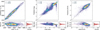 |
Fig. 10 Same as Fig. 8, but showing regression results of the Atmospheric CSWin Parallax-free Framework: Teff (left panel), log g (middle panel), and [Fe/H] (right panel). The color scale from purple to red indicates a gradual increasing probability density, with red areas representing the highest density, where most data points are concentrated. |
5.2 Comparison with magnitudes and colors
Traditionally, stellar atmospheric parameters are derived from the magnitudes of stars. However, in this work, we directly derived them from photometric images using ACF. To demonstrate the superiority of photometric images over magnitudes, we conducted several comparative experiments.
As shown in Sect. 5.1, incorporating parallax information into the framework leads to more precise estimates. To ensure a fair comparison, we also considered parallax and parallax error when using magnitude data. We first obtained the apparent magnitudes of six bands (u, v, g, r, i, and z) from the SMSS DR4 master table. Subsequently, we applied the corresponding interstellar extinction to correct these apparent magnitudes. Following Eq. (17), we converted these apparent magnitudes into absolute magnitudes.
 (17)
(17)
where m0 represents the extinction-corrected apparent magnitude, calculated as m0 = m - A, with m being the uncorrected apparent magnitude and A the interstellar extinction. M0 is the absolute magnitude and  is the parallax in arcseconds.
Furthermore, considering the strong correlation between stellar colors and atmospheric parameters, we also constructed five distinct colors as features: u - v, v - g, g - r, r - i, and i - z. For a given celestial object, the parallax remains the same across different bands. Since color is defined as the difference between magnitudes in two bands, the color derived from absolute magnitudes is identical to that derived from apparent magnitudes because parallax affects both magnitudes equally, and thus cancels out when calculating the colors. As a result, we only need to regress the atmospheric parameters using colors derived from apparent magnitudes, without separately estimating these parameters from colors based on absolute magnitudes.
However, the magnitudes and colors are tabular data and cannot be used directly with the image-specific ACF framework proposed in this paper. Therefore, we employed four commonly used ML algorithms to fit these tabular data, including Random Forest (RF; Breiman 2001), XGBoost (Chen & Guestrin 2016), LightGBM (Ke et al. 2017), and CatBoost (Prokhorenkova et al. 2018). We applied Bayesian optimization to search for the optimal hyperparameters for the four ML algorithms.
This, however, introduces another potential issue-the differences in results may stem from the choice of algorithms rather than intrinsic differences between image-based and magnitude-based (or color-based) data. To ensure comparability, we extracted the 512-dimensional image features from the GAP layer of the ACF backbone. These features were then reduced to 16 dimensions using principal component analysis, and the same four ML algorithms were applied to estimate the three stellar atmospheric parameters. This approach allows for a more direct comparison between image-based and magnitudebased (or color-based) methods, minimizing the influence of algorithmic differences.
Table 1 presents the performance of the four ML algorithms in comparison with our proposed ACF framework. The performance metrics are based on the dispersions in the estimates of three stellar atmospheric parameters: Teff, log g, and [Fe/H]. A lower value indicates that the estimates are closer to the true values, thereby reflecting higher precision. Across all three parameters, the proposed ACF framework consistently achieves the lowest dispersions with or without incorporating parallax information, demonstrating its superior precision. Notably, the incorporation of parallax significantly enhances performance for all algorithms, particularly for the estimation of log g (again confirming the conclusions drawn in Sect. 5.1). While gradient-boosting algorithms such as LightGBM and CatBoost exhibit competitive results for magnitude- and color-based data (e.g., 99.331 K for CatBoost_mag&color with parallax), image-based methods leveraging dimensionality-reduced features consistently outperform tabular data approaches, albeit with marginal percentage-level improvements (2-14%). This modest improvement aligns with theoretical expectations: under ideal PSF characterization, image-based methods cannot exceed the information content encapsulated in PSF magnitudes.
The comparative experiments demonstrate that utilizing photometric images directly yields better atmospheric parameter estimates than relying on magnitudes or colors. This improvement stems from the inherent limitations of traditional magnitude systems, which are susceptible to systematic biases introduced by suboptimal aperture selection and filter-related calibration errors in practical scenarios. These biases propagate through the data reduction pipeline, potentially compromising the precision of derived atmospheric parameters. In contrast, photometric images preserve the original observational information, enabling precise reconstruction of stellar intensity profiles through pixel-level modeling, thereby facilitating more robust atmospheric parameter estimation.
Comparison of different algorithms based on magnitudes, colors, and photometric images.
5.3 Comparison with spectroscopic samples
To further assess the accuracy of stellar atmospheric parameters estimated from photometric images, we compared our estimates with two other spectroscopic surveys: the APOGEE survey and the LAMOST survey.
The APOGEE survey specializes in the H-band portion of the electromagnetic spectrum (1.51-1.70 μm), with a highresolution (R ~ 22 500) and a high signal-to-noise ratio (S/N > 100). The latest data release, APOGEE DR17 (Abdurro’uf et al. 2022), contains measurements of stellar atmospheric parameters and elemental abundances for more than 657 000 stars. It compiles observational data from the APOGEE-1 and APOGEE-2 programs, covering August 2011 to January 2021. APOGEE-2 operates telescopes in both the Northern Hemisphere (APOGEE-2N at Apache Point Observatory, USA) and the Southern Hemisphere (APOGEE-2S at Las Campanas Observatory, Chile), enabling a thorough and wide-ranging observation of the Milky Way. We cross-matched APOGEE DR17 with SMSS DR4 and selected stars with good spectroscopic parameters (i.e., starflag = 0 and fe_h_flag = 0). We note that some samples have low effective temperatures; however, our model lacks sufficient training on such samples. As illustrated in Fig. 1, our training samples are confined to effective temperatures ranging from 4000 K to 8000 K. To ensure the reliability of our predictions, we chose to exclude samples with effective temperatures below 4000 K. This yielded a final sample of 39 550 stars.
A comparison of our stellar atmospheric parameters estimates with those of APOGEE DR17 is shown in Fig. 11. For Teff, the majority of points are distributed along the red dashed one-to-one line. This is particularly noticeable in the region around 5000 K, where the predictions almost align with the spectroscopic estimates of APOGEE DR17. Generally, the predictions for log g show a more compact and consistent distribution, as indicated by the very small dispersion of only 0.13 dex. For [Fe/H], values are overestimated in the metal-poor region ([Fe/H] ⩽ −1) due to the influence of molecular carbon bands, as discussed in Sect. 4.1. Overall, the low dispersion confirms the validity of our photometric estimates.
The Guo Shoujing Telescope, commonly known as LAM-OST, is a Chinese astronomical instrument famous for its high-capacity spectroscopic survey. With a wide field of view enabled by its Schmidt configuration and a 4-meter aperture, LAMOST can simultaneously capture the spectra of thousands of astronomical objects using its 4000 fiber optics system. It operates over a wavelength range of 3700 Å to 9000 Å, offering a resolving power of about R ~ 1800 at 5500 Å. We used stellar atmospheric parameters derived with the LSP3 pipeline (Xiang et al. 2015, 2017), and cross-matched these data with SMSS DR4 to find stars in common. Similarly, we excluded samples beyond the applicable range of effective temperatures to ensure the reliability of our predictions, resulting in a final sample size of 65 319.
Figure 12 illustrates a comparison between our photometric estimates and those reported in LSP3. Although there is a dispersion of approximately 177.73 K in the estimates of Teff, the variation in data density indicates that most photometric predictions are still close to the spectroscopic estimates. For log g, there is some discrepancy between our photometric predictions and the estimates from LSP3, but we still obtain reliable results for stars with low log g. For [Fe/H], the average bias is close to zero and the dispersion is 0.22 dex, indicating that our photometric predictions are in general in agreement with the results of LSP3.
In summary, our method achieves stellar atmospheric parameter predictions that closely align with high-resolution spectroscopic analyses, providing a practical photometric alternative for large stellar samples lacking spectroscopic data.
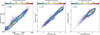 |
Fig. 11 Comparison of photometric estimates of Teff (left panel), log g (middle panel), and [Fe/H] (right panel) with spectroscopic labels from APOGEE DR17. The overall offset (μ) and standard deviation (σ) are indicated in the top-left corner of each panel. Red dashed lines denote the one-to-one lines. Color bars above each panel represent the normalized point density of the results, modeled using kernel density estimation. |
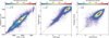 |
Fig. 12 Same as Fig. 11, but comparing photometric estimates of Teff (left panel), log g (middle panel), and [Fe/H] (right panel) with spectroscopic labels from the LSP3 pipeline. |
5.4 Validation on low-quality samples
In Sect. 2.2, we applied strict selection criteria to curate a high-quality sample of 106 145 stars from GALAH+ DR3. However, a significant fraction of astronomical targets in large surveys may fail to meet all quality thresholds due to observational limitations or data artifacts. To evaluate the ACF’s robustness in non-ideal scenarios, we conducted additional experiments on low-quality samples.
We define low-quality samples as those that retain essential criteria ensuring physical validity and model feasibility-spectroscopic parameters reliability (flag_sp = 0, flag_fe_h = 0, and snr_c3_iraf > 30), stellar classification probability (class_star ⩾ 0.6), multiband detection completeness (at least one good detection per filter), and parallax uncertainty (<30%). However, we relaxed nonessential constraints (e.g., Galactic latitude |b| ⩾ 10 , detection quality flags = 0, and minimum neighbor distance of 15 arcseconds). From the full GALAH+ DR3 sample (555 323 stars), we excluded high-quality targets, yielding 190 811 low-quality samples after selection. Similarly, we divided the low-quality samples into training and validation sets in an 8:2 ratio, and the same training strategy was employed to train the model.
The performance evaluation of ACF on the low-quality validation set is summarized in Table 2. Notably, the model demonstrates superior predictive capabilities compared to traditional magnitude-color analysis methods, even when processing degraded input data. As illustrated in Fig. 13, the regression results for the low-quality validation set maintain overall consistency with high-quality counterparts (see Fig. 8). However, the precision shows significant degradation, with the dispersions increasing by 9.25 K for Teff, 0.01 dex for log g, and 0.01 dex for [Fe/H], respectively. However, this highlights the importance of high-quality data in achieving high-precision parameter estimates. In general, the comparative analysis underscores the robustness of the proposed ACF and its ability to generalize to a broader range of data, including low-quality samples.
Comparison of different algorithms based on magnitudes, colors, and photometric images for low-quality samples.
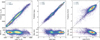 |
Fig. 13 Regression results for three stellar atmospheric parameters in the low-quality validation set: Teff (left panel), log g (middle panel), and [Fe/H] (right panel). The top part of each panel shows spectroscopic labels versus photometric predictions derived using the algorithm described in Sect. 3. The bottom part display the residuals between photometric predictions and spectroscopic labels, with the overall offset (μ) and standard deviation (σ) marked in the top-left corner of top part. To enhance clarity and visualize trends, we use the kernel density estimation method to model the probability densities of the results, represented as a color gradient ranging from purple (low density) to red (high density). Black dashed lines denote the one-to-one relationship, while red dashed lines mark zero residuals in each panel. |
6 Catalog
The experiments presented in Sect. 5.4 demonstrate that the precision of stellar atmospheric parameter predictions from our model strongly depends on photometric image quality. To ensure reliable estimates of stellar atmospheric parameters, we implemented rigorous quality filtering of all SMSS DR4 samples following the criteria outlined in Sect. 2.2. Our selection procedure consisted of multiple stages. First, we applied selection criteria for high-quality stellar sources requiring class_star ⩾ 0.6 and flags = 0. We further imposed the requirement that each star must have at least one valid detection in all photometric bands (u_ngood ⩾ 1, v_ngood ⩾ 1, g_ngood ⩾ 1, r_ngood ⩾ 1, i_ngood ⩾ 1, and z_ngood ⩾ 1) to ensure complete image input. To investigate isolated stellars, we excluded potentially contaminated sources by setting a proximity criterion of self_dist1 = 15 arcseconds. Additionally, we selected stars at Galactic latitude |b| ⩾ 10° to minimize interstellar extinction effects. The combined selection criteria were implemented through the following Astronomical Data Query Language query which is processed by the VO-standard Table Access Protocol in TOPCAT:
SELECT *
FROM dr4.master
WHERE ABS (glat) >=10
AND flags=0
AND class_star >=0. 6
AND u_ngood >=1 AND v_ngood >=1
AND g_ngood >=1 AND r_ngood >=1
AND i_ngood >=1 AND z_ngood >=1
AND self_dist1 =15
This initial selection yielded 10 239 010 candidate stars. Since our framework requires astrometric inputs containing parallaxes and their corresponding errors, we performed a positional cross-match with Gaia EDR3 within a 1-arcsecond matching radius. To ensure measurement reliability, we retained only sources with relative parallax uncertainties below 30%, resulting in a refined sample of 9 178 508 high-quality targets. Given the prohibitive image download times (approximately 13 000 CPU hours) and massive storage requirements (roughly 9 TB) for processing the full sample, we adopted a stratified random sampling approach at a 9:1 ratio, ultimately selecting one million representative stars. The spatial distribution of the final sample (see Fig. 14) demonstrates extensive coverage across the Southern Hemisphere. We then applied the data processing methods described in Sect. 2.3 to generate stacked photometric images. Leveraging the ACF method and training details described in Sect. 3, we derived three atmospheric parameters along with their associated uncertainties for these samples.
Figure 15 presents the distributions of number density and metallicity for one million SMSS DR4 stars in the Teff - log g planes. The density map (logarithmically scaled) highlights a bimodal structure with a high-density locus at Teff ~ 5800 K and logg 4 (characteristic of main-sequence turn-off stars) and a secondary concentration at Teff < 5000 K with log g ~ 2.5 (indicative of red giant branch populations). To better highlight the metallicity variations across different regions, we set the lower limit of the color bar to −2 for the metallicity map. Darker colors indicate lower metallicities, with the darkest regions representing the distribution of metal-poor stars. We also leveraged Gaia EDR3 distances (the inverse of parallaxes) to provide a comprehensive view of the metallicity distribution across the sky. Figure 16 illustrates the spatial distribution of our results, which exhibits a clear radial gradient, with median [Fe/H] values ranging from approximately 0 to below −2. This trend reflects a systematic decline in metallicity from the inner Galactic disk toward the outer regions. Previous studies consistently support this gradient, reporting a higher prevalence of metal-rich stars in the inner Galaxy and a predominance of metal-poor populations in the outer regions (Hayden et al. 2015; Huang et al. 2019).
We further integrated these derived atmospheric parameters into a public catalog. Table 3 enumerates the columns included in this catalog, along with their brief descriptions, and units of measurement (if applicable). Users of this catalog should exercise caution when interpreting results for stars with log g < 1 and [Fe/H] ⩽ −1, as these regimes may require external calibration for robust scientific analyses (described in Sect. 4.1).
 |
Fig. 14 Spatial coverage of the final samples in the Galactic coordinate system. The area between the two gray dashed lines marks regions where Galactic latitude |b| < 10°. This region is excluded from the sample selection. |
Catalog description of stellar atmospheric parameters in SMSS DR4.
7 Conclusions
In this work, we present the ACF, a novel deep learningbased approach for precise estimation of stellar atmospheric parameters. The ACF was designed as a dual-input architecture that combines astrometric inputs (parallaxes and their errors) that provide distance information and photometric image inputs to preserve complete stellar observational information. We employed the CSWin Transformer as the image backbone network to maximize stellar feature extraction and utilize MC dropout in the prediction module for robust uncertainty quantification. Our key findings and contributions are summarized as follows:
- (1)
High-precision parameter estimation: The ACF demonstrates high precision on the validation set, with dispersions of 95.02 K for Teff, 0.07 dex for log g, and 0.14 dex for [Fe/H], approaching the precision of high-resolution spectroscopic analyses.
- (2)
Critical role of astrometric data: Systematic experiments confirm that incorporating Gaia parallaxes significantly enhances the accuracy of the parameters, particularly for log g (which is improved by up to 75%).
- (3)
Superiority of image features: Our image-based methods outperform traditional approaches relying on stellar magnitudes or colors, with improvements ranging from 2% to 14%. This demonstrates the potential of image-based deep learning as a powerful alternative to traditional magnitude-or color-dependent approaches.
- (4)
Robustness and generalizability: The ACF’s dual-input architecture, coupled with MC dropout for uncertainty quantification, ensures reliable predictions even for low-quality photometric samples.
- (5)
Community resource: We publicly released a catalog of atmospheric parameters for one million SMSS DR4 stars, providing a new dataset for Galactic archaeology.
It should be noted that while the improvement achieved in this study may appear marginal at the theoretical level (given that the majority of stars can be effectively characterized as pointlike sources convolved with the PSF), the innovative value of this research is reflected in its practical application. First, in large-scale sky surveys, even marginal improvements in individual stellar parameter precision, when accumulated across tens of thousands of stellar samples, can significantly enhance the reliability of statistical results. Second, under non-ideal observing conditions, where traditional aperture photometry is vulnerable to contamination from neighboring stars, our image-based modeling approach effectively mitigates such interference. Most importantly, for astrophysically interesting systems such as close binary stars with sub-pixel-scale structures, our method can capture photometric details that are inaccessible to conventional magnitude systems, opening new avenues for studying complex stellar systems.
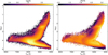 |
Fig. 15 Distributions of number density (left panel) and metallicity (right panel) for one million SMSS DR4 stars in the Teff - log g planes. Both panels are computed using bins of 25 K in Teff and 0.04 dex in log g, with color bars above each panel indicating the corresponding values. Number densities are shown on a logarithmic scale, while metallicities are represented by the median values within the bins. The lower limit of the right color bar is set to −2, so all metallicity values below −2 are shown in the same color as −2. |
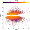 |
Fig. 16 Median metallicity distribution in the R-z plane for one million SMSS DR4 stars, binned into 0.2 × 0.15 kpc2. Here, R represents the cylindrical Galactocentric distance and z denotes the distance to the Galactic plane. The color bar shows the metallicity values, with a lower limit set to −2 to better illustrate variations with Galactic position. |
Data availability
The catalog is available at the CDS via anonymous ftp to cdsarc.cds.unistra.fr (130.79.128.5) or via https://cdsarc.cds.unistra.fr/viz-bin/cat/J/A+A/698/A322. It is also available through the Zenodo repository at https://zenodo.org/records/15315249.
Acknowledgements
We thank the anonymous referee for useful comments that helped us improve the manuscript substantially. We would also like to thank Haibo Yuan for helpful discussions on data processing. This work is supported by the Natural Science Foundation of Shandong Province under grants Nos. ZR2024MA063, ZR2022MA076, and ZR2022MA089, the National Natural Science Foundation of China (NSFC) under grant No. 11873037, the science research grants from the China Manned Space Project with No. CMS-CSST-2021-B05 and CMS-CSST-2021-A08, and is partially supported by the Young Scholars Program of Shandong University, Weihai (2016WHWLJH09). X.K is supported by the National Natural Science Foundation of China under grant No. 11803016. The national facility capability for SkyMapper has been funded through ARC LIEF grant LE130100104 from the Australian Research Council, awarded to the University of Sydney, the Australian National University, Swinburne University of Technology, the University of Queensland, the University of Western Australia, the University of Melbourne, Curtin University of Technology, Monash University and the Australian Astronomical Observatory. SkyMapper is owned and operated by The Australian National University’s Research School of Astronomy and Astrophysics. The survey data were processed and provided by the SkyMapper Team at ANU. The SkyMapper node of the All-Sky Virtual Observatory (ASVO) is hosted at the National Computational Infrastructure (NCI). Development and support of the SkyMapper node of the ASVO has been funded in part by Astronomy Australia Limited (AAL) and the Australian Government through the Commonwealth’s Education Investment Fund (EIF) and National Collaborative Research Infrastructure Strategy (NCRIS), particularly the National eResearch Collaboration Tools and Resources (NeCTAR) and the Australian National Data Service Projects (ANDS). This work made use of the Third Data Release of the GALAH Survey (Buder et al. 2021). The GALAH Survey is based on data acquired through the Australian Astronomical Observatory, under programs: A/2013B/13 (The GALAH pilot survey); A/2014A/25, A/2015A/19, A2017A/18 (The GALAH survey phase 1); A2018A/18 (Open clusters with HERMES); A2019A/1 (Hierarchical star formation in Ori OB1); A2019A/15 (The GALAH survey phase 2); A/2015B/19, A/2016A/22, A/2016B/10, A/2017B/16, A/2018B/15 (The HERMES-TESS program); and A/2015A/3, A/2015B/1, A/2015B/19, A/2016A/22, A/2016B/12, A/2017A/14 (The HERMES K2-follow-up program). We acknowledge the traditional owners of the land on which the AAT stands, the Gamilaraay people, and pay our respects to elders past and present. This paper includes data that has been provided by AAO Data Central (datacentral.org.au). Funding for the Sloan Digital Sky Survey IV has been provided by the Alfred P. Sloan Foundation, the US Department of Energy Office of Science, and the Participating Institutions. SDSS acknowledges support and resources from the Center for High-Performance Computing at the University of Utah. The SDSS website is www.sdss.org. SDSS is managed by the Astrophysical Research Consortium for the Participating Institutions of the SDSS Collaboration including the Brazilian Participation Group, the Carnegie Institution for Science, Carnegie Mellon University, Center for Astrophysics | Harvard & Smithsonian (CfA), the Chilean Participation Group, the French Participation Group, Instituto de Astrofísica de Canarias, The Johns Hopkins University, Kavli Institute for the Physics and Mathematics of the Universe (IPMU) / University of Tokyo, the Korean Participation Group, Lawrence Berkeley National Laboratory, Leibniz Institut für Astrophysik Potsdam (AIP), Max-Planck-Institut für Astronomie (MPIA Heidelberg), Max-Planck-Institut für Astrophysik (MPA Garching), Max-Planck-Institut für Extraterrestrische Physik (MPE), National Astronomical Observatories of China, New Mexico State University, New York University, University of Notre Dame, Observatório Nacional / MCTI, The Ohio State University, Pennsylvania State University, Shanghai Astronomical Observatory, United Kingdom Participation Group, Universidad Nacional Autónoma de México, University of Arizona, University of Colorado Boulder, University of Oxford, University of Portsmouth, University of Utah, University of Virginia, University of Washington, University of Wisconsin, Vanderbilt University, and Yale University. Guoshoujing Telescope (the Large Sky Area Multi-Object Fiber Spectroscopic Telescope LAMOST) is a National Major Scientific Project built by the Chinese Academy of Sciences. Funding for the project has been provided by the National Development and Reform Commission. LAMOST is operated and managed by the National Astronomical Observatories, Chinese Academy of Sciences. This work has made use of data from the European Space Agency (ESA) mission Gaia (https://www.cosmos.esa.int/gaia), processed by the Gaia Data Processing and Analysis Consortium (DPAC, https://www.cosmos.esa.int/web/gaia/dpac/consortium). Funding for the DPAC has been provided by national institutions, in particular the institutions participating in the Gaia Multilateral Agreement.
References
- Abdurro’uf, Accetta K., Aerts, C., et al. 2022, ApJS, 259, 35 [NASA ADS] [CrossRef] [Google Scholar]
- Andrae, R., Rix, H.-W., & Chandra, V. 2023, ApJS, 267, 8 [NASA ADS] [CrossRef] [Google Scholar]
- Arcelin, B., Doux, C., Aubourg, E., Roucelle, C., & LSST Dark Energy Science Collaboration. 2021, MNRAS, 500, 531 [Google Scholar]
- Bailer-Jones, C. A. L. 2015, PASP, 127, 994 [Google Scholar]
- Bessell, M. S. 2005, ARA&A, 43, 293 [NASA ADS] [CrossRef] [Google Scholar]
- Breiman, L. 2001, Mach. Learn., 45, 5 [Google Scholar]
- Bu, Y., & Pan, J. 2015, MNRAS, 447, 256 [Google Scholar]
- Buder, S., Sharma, S., Kos, J., et al. 2021, MNRAS, 506, 150 [NASA ADS] [CrossRef] [Google Scholar]
- Buntine, W. 1991, in Uncertainty Proceedings 1991 (Elsevier), 52 [CrossRef] [Google Scholar]
- Cantat-Gaudin, T., Anders, F., Castro-Ginard, A., et al. 2020, A&A, 640, A1 [NASA ADS] [CrossRef] [EDP Sciences] [Google Scholar]
- Casagrande, L., Wolf, C., Mackey, A. D., et al. 2019, MNRAS, 482, 2770 [NASA ADS] [Google Scholar]
- Chambers, K. C., Magnier, E. A., Metcalfe, N., et al. 2016, arXiv e-prints [arXiv:1612.05560] [Google Scholar]
- Chen, T., & Guestrin, C. 2016, arXiv e-prints [arXiv:1603.02754] [Google Scholar]
- De Silva, G. M., Freeman, K. C., Bland-Hawthorn, J., et al. 2015, MNRAS, 449, 2604 [NASA ADS] [CrossRef] [Google Scholar]
- Deng, L., Newberg, H. J., Liu, C., et al. 2012, Res. Astron. Astrophys., 12, 735 [Google Scholar]
- Dey, B., Andrews, B. H., Newman, J. A., et al. 2022, MNRAS, 515, 5285 [NASA ADS] [CrossRef] [Google Scholar]
- Dong, X., Bao, J., Chen, D., et al. 2022, in Proceedings of the IEEE/CVF Conference on Computer Vision and Pattern Recognition, 12124 [Google Scholar]
- Gaia Collaboration (Brown, A. G. A., et al.) 2016, A&A, 595, A2 [NASA ADS] [CrossRef] [EDP Sciences] [Google Scholar]
- Gaia Collaboration (Brown, A. G. A., et al.) 2018, A&A, 616, A1 [NASA ADS] [CrossRef] [EDP Sciences] [Google Scholar]
- Gaia Collaboration (Brown, A. G. A., et al.) 2021, A&A, 649, A1 [NASA ADS] [CrossRef] [EDP Sciences] [Google Scholar]
- Gal, Y., & Ghahramani, Z. 2016, in International Conference on Machine Learning, PMLR, 1050 [Google Scholar]
- Gilmore, G., Randich, S., Worley, C. C., et al. 2022, A&A, 666, A120 [NASA ADS] [CrossRef] [EDP Sciences] [Google Scholar]
- Graves, A. 2011, in Advances in Neural Information Processing Systems, 24 [Google Scholar]
- Hayden, M. R., Bovy, J., Holtzman, J. A., et al. 2015, ApJ, 808, 132 [Google Scholar]
- He, Z., Qiu, B., Luo, A. L., et al. 2021, MNRAS, 508, 2039 [NASA ADS] [CrossRef] [Google Scholar]
- Huang, Y., Chen, B. Q., Yuan, H. B., et al. 2019, ApJS, 243, 7 [CrossRef] [Google Scholar]
- Huang, Y., Beers, T. C., Xiao, K., et al. 2024, ApJ, 974, 192 [Google Scholar]
- IveziC, ., Sesar, B., Juric, M., et al. 2008, ApJ, 684, 287 [NASA ADS] [CrossRef] [Google Scholar]
- Ke, G., Meng, Q., Finley, T., et al. 2017, Adv. Neural Inform. Process. Syst., 30 [Google Scholar]
- Khalatyan, A., Anders, F., Chiappini, C., et al. 2024, A&A, 691, A98 [NASA ADS] [CrossRef] [EDP Sciences] [Google Scholar]
- Kim, B., & Lépine, S. 2022, MNRAS, 510, 4308 [NASA ADS] [CrossRef] [Google Scholar]
- Liang, J., Bu, Y., Tan, K., et al. 2022, AJ, 163, 153 [NASA ADS] [CrossRef] [Google Scholar]
- Liu, X. W., Yuan, H. B., Huo, Z. Y., et al. 2014, in Setting the Scene for Gaia and LAMOST, 298, eds. S. Feltzing, G. Zhao, N. A. Walton, & P. Whitelock, 310 [Google Scholar]
- Luri, X., Brown, A. G. A., Sarro, L. M., et al. 2018, A&A, 616, A9 [NASA ADS] [CrossRef] [EDP Sciences] [Google Scholar]
- Luvaul, L. C., Onken, C. A., Wolf, C., Smillie, J. G., & Sebo, K. M. 2017, in Astronomical Society of the Pacific Conference Series, 512, Astronomical Data Analysis Software and Systems XXV, eds. N. P. F. Lorente, K. Shortridge, & R. Wayth, 393 [Google Scholar]
- MacKay, D. J. 1992, Neural Computat., 4, 448 [Google Scholar]
- Majewski, S. R., Schiavon, R. P., Frinchaboy, P. M., et al. 2017, AJ, 154, 94 [NASA ADS] [CrossRef] [Google Scholar]
- Matteucci, F. 2021, A&A Rev., 29, 5 [NASA ADS] [CrossRef] [Google Scholar]
- McClure, R. D. 1976, AJ, 81, 182 [Google Scholar]
- Ness, M., Hogg, D. W., Rix, H. W., Ho, A. Y. Q., & Zasowski, G. 2015, ApJ, 808, 16 [NASA ADS] [CrossRef] [Google Scholar]
- Onken, C. A., Wolf, C., Bessell, M. S., et al. 2019, PASA, 36, e033 [Google Scholar]
- Onken, C. A., Wolf, C., Bessell, M. S., et al. 2024, PASA, 41, e061 [NASA ADS] [CrossRef] [Google Scholar]
- Pence, W. D., Chiappetti, L., Page, C. G., Shaw, R. A., & Stobie, E. 2010, A&A, 524, A42 [NASA ADS] [CrossRef] [EDP Sciences] [Google Scholar]
- Piskunov, N., & Valenti, J. A. 2017, A&A, 597, A16 [NASA ADS] [CrossRef] [EDP Sciences] [Google Scholar]
- Prokhorenkova, L., Gusev, G., Vorobev, A., Dorogush, A. V., & Gulin, A. 2018, Adv. Neural Inform. Process. Syst., 31 [Google Scholar]
- Randich, S., Gilmore, G., Magrini, L., et al. 2022, A&A, 666, A121 [NASA ADS] [CrossRef] [EDP Sciences] [Google Scholar]
- Robin, A. C., Reylé, C., Derrière, S., & Picaud, S. 2003, A&A, 409, 523 [NASA ADS] [CrossRef] [EDP Sciences] [Google Scholar]
- Rockosi, C. M., Lee, Y. S., Morrison, H. L., et al. 2022, ApJS, 259, 60 [CrossRef] [Google Scholar]
- Schlegel, D. J., Finkbeiner, D. P., & Davis, M. 1998, ApJ, 500, 525 [Google Scholar]
- Skrutskie, M. F., Cutri, R. M., Stiening, R., et al. 2006, AJ, 131, 1163 [NASA ADS] [CrossRef] [Google Scholar]
- Soubiran, C., Brouillet, N., & Casamiquela, L. 2022, A&A, 663, A4 [NASA ADS] [CrossRef] [EDP Sciences] [Google Scholar]
- Steinmetz, M., Zwitter, T., Siebert, A., et al. 2006, AJ, 132, 1645 [Google Scholar]
- Stromgren, B. 1951, AJ, 56, 174 [Google Scholar]
- Tabernero, H. M., Marfil, E., Montes, D., & González Hernández, J. I. 2022, A&A, 657, A66 [NASA ADS] [CrossRef] [EDP Sciences] [Google Scholar]
- Ting, Y.-S. 2024, arXiv e-prints [arXiv:2412.05806] [Google Scholar]
- Valenti, J. A., & Piskunov, N. 1996, A&AS, 118, 595 [NASA ADS] [CrossRef] [EDP Sciences] [Google Scholar]
- Vaswani, A., Shazeer, N., Parmar, N., et al. 2017, arXiv e-prints [arXiv:1706.03762] [Google Scholar]
- Wolf, C., Luvaul, L. C., Onken, C. A., Smillie, J. G., & White, M. C. 2017, in Astronomical Society of the Pacific Conference Series, 512, Astronomical Data Analysis Software and Systems XXV, eds. N. P. F. Lorente, K. Shortridge, & R. Wayth, 289 [Google Scholar]
- Wolf, C., Onken, C. A., Luvaul, L. C., et al. 2018, PASA, 35, e010 [Google Scholar]
- Wright, E. L., Eisenhardt, P. R. M., Mainzer, A. K., et al. 2010, AJ, 140, 1868 [Google Scholar]
- Wu, F., Bu, Y., Zhang, M., et al. 2023, AJ, 166, 88 [NASA ADS] [CrossRef] [Google Scholar]
- Xiang, M. S., Liu, X. W., Yuan, H. B., et al. 2015, MNRAS, 448, 822 [NASA ADS] [CrossRef] [Google Scholar]
- Xiang, M., Liu, X., Yuan, H., et al. 2017, MNRAS, 467, 1890 [Google Scholar]
- Yang, H., Yin, X., Cai, J., et al. 2023, Res. Astron. Astrophys., 23, 055006 [CrossRef] [Google Scholar]
- Yang, L., Yuan, H., Xiang, M., et al. 2022, A&A, 659, A181 [NASA ADS] [CrossRef] [EDP Sciences] [Google Scholar]
- Yanny, B., Rockosi, C., Newberg, H. J., et al. 2009, AJ, 137, 4377 [Google Scholar]
- York, D. G., Adelman, J., Anderson, John E. J., et al. 2000, AJ, 120, 1579 [NASA ADS] [CrossRef] [Google Scholar]
- Yuan, H., Liu, X., Xiang, M., Huang, Y., & Chen, B. 2015, ApJ, 803, 13 [CrossRef] [Google Scholar]
- Zheng, J., Zhao, G., Wang, W., et al. 2018, Res. Astron. Astrophys., 18, 147 [CrossRef] [Google Scholar]
Catalog available at the GALAH+ DR3 repository: https://cloud.datacentral.org.au/teamdata/GALAH/public/GALAH_DR3/
All Tables
Comparison of different algorithms based on magnitudes, colors, and photometric images.
Comparison of different algorithms based on magnitudes, colors, and photometric images for low-quality samples.
All Figures
|
Fig. 1 Distribution of samples in the Teff−log g plane (left) and the Teff−[Fe/H] plane (right). Black and red dots represent the training and validation sets, respectively, with a ratio of 8:2. |
| In the text | |
|
Fig. 2 Visualization of the data processing procedure. The “Original” panel displays the raw photometric images of a target object across six bands (u, v, g, r, i, and z) from the SMSS DR4, where each band can include multiple detections. For clarity, only two representative detections are shown. The “Corrected” panel shows the photometric images after applying zeropoint and reddening corrections. Subsequently, image reprojection is performed to achieve precise spatial alignment, as demonstrated in the “Aligned” panel. Finally, the “Stacked” panel presents the stacked photometric images generated through a simple averaging method. |
| In the text | |
|
Fig. 3 Illustration of the standard self-attention mechanism. The input matrix X of size L Demb is transformed into the query (Q), key (K), and value (V) matrices, each of size L Dout, through weight matrices WQ, WK, and WV. The attention matrix A is computed by taking the dot product of Q and K, followed by a softmax operation. The final output Y of size L Dout is obtained by multiplying A with V. |
| In the text | |
|
Fig. 4 Illustration of the cross-shaped window self-attention. A feature map of shape H W C is first linearly projected to K heads. This is then split into Group A and Group B to calculate horizontal and vertical self-attention in parallel. Finally, the outputs of the two groups are concatenated to obtain the cross-shaped window self-attention. |
| In the text | |
|
Fig. 5 Structure of the CSWin Transformer block. The CSWin-Attention refers to cross-shaped window self-attention, which is detailed in Sect. 3.1.2. |
| In the text | |
|
Fig. 6 Parallax distribution on a logarithmic scale for all samples. The black line and red dashed line represent the training and validation sets, respectively. |
| In the text | |
|
Fig. 7 Architecture of the Atmospheric CSWin Framework used for regression tasks. The framework employed a dual-input architecture to process both astrometric and photometric data. The astrometric branch (top left, gray frame) took parallaxes and their associated errors as input. These parameters were jointly encoded through a 128-dimensional fully connected layer. In parallel, the photometric branch (middle left, pink frame) processed six-band (u, v, g, r, i, and z) images with dimensions 48 × 48 × 6. These images were fed into a CSWin Transformer backbone network (bottom, pink frame), which performed hierarchical feature extraction across four progressive stages. Each stage contained multiple CSWin Transformer blocks, which captured both local and global spatial information through CSWin-Attention mechanism. Through this process, the backbone generated a 512-dimensional visual feature representation. The framework then combined these complementary representations through concatenation (denoted by ©) to form a 640-dimensional composite feature vector. This fused feature vector served as input to the prediction module (top right, orange frame), which consisted of three fully connected layers incorporating MC dropout. The expected value of multiple sampled outputs from the prediction module, denoted as E(Yh), served as the model’s prediction y* (i.e., Teff, log g, or [Fe/H]). The variance of these sampled outputs, denoted as D(Yh), was used to assess the uncertainty σ* of the model’s prediction. |
| In the text | |
|
Fig. 8 Regression results for three stellar atmospheric parameters in the validation set: Teff (left panel), log g (middle panel), and [Fe/H] (right panel). The top part of each panel show spectroscopic labels versus photometric predictions derived using the algorithm described in Sect. 3. The lower-left part of each panel displays the residuals between photometric predictions and spectroscopic labels, with the overall offset (μ) and standard deviation (σ) indicated in the top-left corner of the top plot. To enhance clarity and visualize trends, kernel density estimation (KDE) is used to model the probability densities of the results, represented as a color gradient ranging from purple (low density) to red (high density). The lower-right part of each panel shows the probability density of the residuals fitted using KDE. Black dashed lines denote the one-to-one relationship, while red dashed lines mark zero residuals. |
| In the text | |
|
Fig. 9 Model uncertainties for three stellar atmospheric parameters: Teff (left panel), log g (middle panel), and [Fe/H] (right panel). Kernel density estimation (KDE) is used to approximate the probability density functions of model uncertainties. Areas of darker color represent regions of lower probability densities, while lighter areas indicate higher probability densities. The red solid lines show second-order polynomial regression curves, that delineate the trend between uncertainties and atmospheric parameters. The red shaded area corresponds to the 95% confidence interval of the regression. Its width represents the size of confidence interval and the variation reflects changes in predictive uncertainty as a function of atmospheric parameters. |
| In the text | |
|
Fig. 10 Same as Fig. 8, but showing regression results of the Atmospheric CSWin Parallax-free Framework: Teff (left panel), log g (middle panel), and [Fe/H] (right panel). The color scale from purple to red indicates a gradual increasing probability density, with red areas representing the highest density, where most data points are concentrated. |
| In the text | |
|
Fig. 11 Comparison of photometric estimates of Teff (left panel), log g (middle panel), and [Fe/H] (right panel) with spectroscopic labels from APOGEE DR17. The overall offset (μ) and standard deviation (σ) are indicated in the top-left corner of each panel. Red dashed lines denote the one-to-one lines. Color bars above each panel represent the normalized point density of the results, modeled using kernel density estimation. |
| In the text | |
|
Fig. 12 Same as Fig. 11, but comparing photometric estimates of Teff (left panel), log g (middle panel), and [Fe/H] (right panel) with spectroscopic labels from the LSP3 pipeline. |
| In the text | |
|
Fig. 13 Regression results for three stellar atmospheric parameters in the low-quality validation set: Teff (left panel), log g (middle panel), and [Fe/H] (right panel). The top part of each panel shows spectroscopic labels versus photometric predictions derived using the algorithm described in Sect. 3. The bottom part display the residuals between photometric predictions and spectroscopic labels, with the overall offset (μ) and standard deviation (σ) marked in the top-left corner of top part. To enhance clarity and visualize trends, we use the kernel density estimation method to model the probability densities of the results, represented as a color gradient ranging from purple (low density) to red (high density). Black dashed lines denote the one-to-one relationship, while red dashed lines mark zero residuals in each panel. |
| In the text | |
|
Fig. 14 Spatial coverage of the final samples in the Galactic coordinate system. The area between the two gray dashed lines marks regions where Galactic latitude |b| < 10°. This region is excluded from the sample selection. |
| In the text | |
|
Fig. 15 Distributions of number density (left panel) and metallicity (right panel) for one million SMSS DR4 stars in the Teff - log g planes. Both panels are computed using bins of 25 K in Teff and 0.04 dex in log g, with color bars above each panel indicating the corresponding values. Number densities are shown on a logarithmic scale, while metallicities are represented by the median values within the bins. The lower limit of the right color bar is set to −2, so all metallicity values below −2 are shown in the same color as −2. |
| In the text | |
|
Fig. 16 Median metallicity distribution in the R-z plane for one million SMSS DR4 stars, binned into 0.2 × 0.15 kpc2. Here, R represents the cylindrical Galactocentric distance and z denotes the distance to the Galactic plane. The color bar shows the metallicity values, with a lower limit set to −2 to better illustrate variations with Galactic position. |
| In the text | |
Current usage metrics show cumulative count of Article Views (full-text article views including HTML views, PDF and ePub downloads, according to the available data) and Abstracts Views on Vision4Press platform.
Data correspond to usage on the plateform after 2015. The current usage metrics is available 48-96 hours after online publication and is updated daily on week days.
Initial download of the metrics may take a while.