© The Authors 2025

1. Introduction

The chemistry of the early Universe has been the target of large studies aimed at determining the abundances of elements and dedicated to the calculation of reaction rates that govern chemical processes, which are contingent on the prevailing environmental conditions. Such investigations explore the primordial species produced by the first nuclear reactions during standard Big Bang nucleosynthesis (SBBN), (see e.g., Workman 2022; Signore & Puy 2009; Cyburt et al. 2016; Pitrou et al. 2021; Schöneberg 2024), up to the interstellar medium (ISM), hosting a variety of heavier elements forged within stars (Tielens 2005; Herbst 1995).

From the SBBN, the Universe was completely ionized, as the temperature of the baryon-photon fluid, maintained by interactions via Compton scattering between free electrons and photons, was too high for any neutral atom to form. However, as the Universe expanded, the effectiveness of baryon-radiation coupling diminished, allowing ion-electron reactions to dominate. Consequently, this led to the progressive recombination of ionized elemental forms into their neutral counterparts (Zeldovich et al. 1968; Peebles 1968). Simultaneously, despite their much lower reaction rates due to the necessarily high amount of energy for these processes to happen, molecules also began to form (Puy et al. 1993).

Species abundance estimation is a central problem of any coupled reaction network. One of the first detailed models of molecular synthesis were proposed by Solomon & Klemperer (1972), who computed molecular abundances in diffuse interstellar clouds, and by Herbst & Klemperer (1973) who studied the formation of molecules in dense dark clouds. The article of Prasad & Huntress (1980), which gave a comprehensive library consisting of over 1400 reactions for 137 species, presented a first model for gas phase chemistry in interstellar clouds. The UMIST Database (Le Teuff et al. 2000; McElroy et al. 2013), contains the updated rate coefficient, temperature ranges and temperature dependence of 6173 gas-phase reactions important in astrophysical environments. However at early epochs, when a total absence of dust grains appears justified, the chemistry is different from the typical interstellar medium chemistry. From the exhaustive work of Bates (1951) on the radiative association rate, Takayanagi & Nishimura (1960), Hirasawa (1969), Takeda et al. (1969), Saslaw & Zipoy (1967) and Matsuda et al. (1969) pointed out the way of H₂ formation through H${}_2^{+}$ and H⁻ without grains in the early Universe. Several chemical networks studies including the primordial molecules (such as H₂, HD, and LiH) and ions were carried out by Lepp & Shull (1984), Latter & Black (1991), Puy et al. (1993), Galli & Palla (1998), Stancil & Dalgarno (1998), Lepp et al. (2002), Pfenniger & Puy (2003), Hirata & Padmanabhan (2006), Glover & Abel (2008), Signore & Puy (2009), Coppola et al. (2011, 2012, 2013), Gay et al. (2011).

The determination of the molecular abundances is essential in the study of the formation of structures. Indeed, the excitation of the rotational and vibrational levels of the molecules inside collapsing matter overdensities gives rise to a molecular cooling mechanism, which can induce the appearance of instabilities of a thermal nature, highlighted for the first time in Field (1965) and later in Yoshii & Sabano (1980). This excitation is necessary in order to trigger the formation of the first stars Tegmark et al. (1997), Puy & Signore (1997), Yoshida et al. (2006), Trenti & Stiavelli (2009), Galli & Palla (2013), Bromm (2013), Glover (2012), Ripamonti & Abel (2004). Molecular cooling has been extensively studied for numerous molecular species, the most important being H₂, which despite the absence of a dipole moment is the stronger coolant due to its high abundance (Abel et al. 1997; Galli & Palla 1998; Stancil et al. 1998; Glover & Abel 2008). HD is also expected to be an efficient coolant due to its non-zero dipole moment, but it has been shown that it only dominates the molecular cooling at very low temperatures (∼150 K; Glover & Abel 2008), which are typically not reached in primordial gas during the collapse of the first overdense regions (Bromm et al. 2002). Other early molecules, such as H${}_2^{+}$ (Yoshida et al. 2007; Glover & Savin 2009), H${}_3^{+}$ (Glover & Savin 2006, 2009), and LiH (Stancil et al. 1996; Mizusawa et al. 2005), have minor cooling contributions in the context of setting up the conditions for the formation of the first stars.

Probing the formation of the first structures preceding star formation, during the so-called dark ages, is very challenging because almost no signals are emitted from this epoch. Baryonic matter predominantly existed in a neutral state, as the Compton coupling with radiation waned with cosmic expansion. The 21 cm hydrogen line, arising from hyperfine spin-flip transitions in neutral hydrogen atoms, offers a promising avenue for probing this epoch.

Many future experiments are planned in order to measure the 21 cm signal during cosmic dawn and the Epoch of Reionization, such as Experiment to Detect the Global rEionization Signature (EDGES; Bowman et al. 2018), Shaped Antenna measurement of the background RAdio Spectrum (SARAS; Nambissan et al. 2021), Large-Aperture Experiment to Detect the Dark Ages (LEDA; Price et al. 2018), the Radio Experiment for the Analysis of Cosmic Hydrogen (REACH; de Lera Acedo et al. 2022), and Probing Radio Intensity at high-Z from Marion (PRizM; Philip et al. 2019). These studies are aimed at the observation of the 21 cm global signal, whereas ground based interferometers such as the Hydrogen Epoch of Reionization Array (HERA; DeBoer 2017), Low Frequency Array (LOFAR; van Haarlem et al. 2013; Patil et al. 2016), Murchison Widefield Array (MWA; Bowman et al. 2013; Tingay et al. 2013; Jacobs et al. 2016), the Giant Metrewave Radio Telescope (GMRT; Swarup et al. 1991), the Precision Array for Probing the Epoch of Reionization (PAPER; Parsons et al. 2010), and the future Square Kilometer Array (SKA; Koopmans et al. 2015) are measuring or planning to measure the spatial fluctuations in the signal.

However, the observation of the redshifted 21 cm power spectrum and global signal from the dark ages is extremely challenging and cannot be done from Earth-based experiments, because of the ionosphere which acts as a highly opaque foreground for the frequencies of interest, as well as the radio frequency interferences of human origin. The greatest hopes to fathom the dark ages are placed on space missions, either in orbit around the Moon, with the satellites and nanosatellites. We also refer to Burns et al. (2021a) and Fialkov et al. (2024), DSL (Shi et al. 2022), NCDL (Bentum et al. 2020), and CosmoCube (Artuc & de Lera Acedo 2024), or directly on the Moon's surface with ROLSES (Burns et al. 2021b), LuSEE-Night (Bale et al. 2023), the Lunar Crater Radio Telescope (Goel et al. 2022), FarView (Polidan et al. 2024), the Astronomical Lunar Observatory (ALO; Klein Wolt et al. 2024), FARSIDE (Burns et al. 2021b), and LARAF (Chen et al. 2024). A mission with similar objectives, known as Primordial Hydrogen Observation with Nanosatellites Explorer (PHONE), is also in co-development by the Laboratoire Univers et Particules de Montpellier (LUPM) and the Spatial Center, dedicated to the development of nanosatellites, at the University of Montpellier.

Our work takes part in the studies of the 21 cm signal from minihalos. However, unlike aforementioned works, which concentrate on estimating the signal from halos that have already been virialized, we focus on the earlier stages, from the turnaround point of an overdense region, to the end of its collapse. In particular, we aim to highlight the impact of molecular cooling on the 21 cm signal arising from the halos.

The originality of this work lies in coupling the evolution of interactions between atomic and molecular ions, neutral atoms, and molecules with the dynamic and thermal evolution of a medium undergoing gravitational collapse. While this context has been extensively studied in the past to understand the fragmentation of a molecular cloud by the process of thermal instability, in this article, we integrated the calculation of the emissivity of the excitation process of neutral hydrogen producing a hyperfine transition and followed “step by step” this emissivity during a collapse. This coupled approach enables us to predict the emissivity of the 21 cm line at high redshifts. This work is part of a large body of research into the production of the 21 cm line during the cosmological dark ages.

Numerous studies have been carried out to characterize the first structures with 21 cm hydrogen line, before the formation of the first stars. Iliev et al. (2002) proposed a model of 21 cm emission in minihalos from collisional excitation, before reionization. Meiksin (2011) followed spherical collapsing density perturbations, estimating the 21 cm signature arising from the fully collapsed minihalos accounting for the effects of molecular hydrogen formation. A statistical 21 cm signal from the halo has been provided, demonstrating how this signature could distinguish predictions of the small scales of the 21 cm power spectrum. Furugori et al. (2020) calculated the 21 cm signal emitted by ultracompact minihalos formed at high redshift. Novosyadlyj et al. (2020) calculated the 21 cm emission in halos between 10⁶ and 10¹⁰ M_⊙, virialized between z∼10−50. Recently, Novosyadlyj et al. (2025) estimated the global signal in the redshifted hyperfine structure line 21 cm of hydrogen atoms formed during the dark ages and cosmic dawn. They show that the profile of this line crucially depends on the temperature and ionization of baryonic matter as well as the spectral energy distribution of radiation from the first sources.

In this paper, we make use of the code CHEMFAST initiated by Puy et al. (1993), Pfenniger & Puy (2003) and Vonlanthen et al. (2009). The original purpose of this code is to compute the abundances of atomic and molecular species in the context of cosmological expansion of the universe. We incorporated the computation of the global 21 cm line signal arising from collisional coupling during the dark ages. Then, by changing the equations of dynamics in the code, we followed a collapse scenario of a 10⁶−10⁹ M_⊙ overdense region, modeling the region with a simple homogeneous spherical model, including pressure effects (Lahav 1986; Puy & Signore 1996). We emphasized the cooling effects on the gas temperature, arising from molecular excitation during the collapse. We additionally computed the 21 cm signal from the forming protocloud, highlighting its distinct features compared to the expected sky-averaged 21 cm global signal.

This paper is organized as follows. In Sect. 2, we start by developing the reaction network and equations of dynamics in the context of expanding homogeneous Universe. We present the CHEMFAST code computation of atomic and molecular abundances. In Sect. 3, we introduce the physics of the 21 cm global signal during the dark ages. In Sect. 4, we describe the dynamics of the spherical collapse model and, finally, we present our analysis of the thermal and 21 cm signal evolution in collapsing halos in Sect. 5. We present our conclusions and outline our future research directions in Sect. 6. Throughout this paper, we adopted the ΛCDM cosmology, using the parameters values from Planck2018 Planck Collaboration VI (2020) TT,TE,EE+lowE+lensing best-fit.

2. CHEMFAST in homogeneous universe

In this section, we consider the well-studied case of the background evolution of chemistry during the recombination and the dark ages. Our aim is to present how the code works using this example, and to introduce the concepts that will also be employed in this study.

In CHEMFAST, we follow a system of coupled differential equations in order to track the evolution of species abundances. The SBBN model for the Universe predicts the nuclei abundances of mainly hydrogen, helium, and lithium as well as their isotopes. The chemistry of the early Universe is the chemistry of these light elements and their respective isotopic forms. The ongoing physical reactions are numerous after the nucleus recombination. These reactions fall into three distinct categories:

• Collisional reactions ξ+ξ′⟷ξ₁+ξ₂ involve processes such as association, associative detachment, mutual neutralization, charge exchange, and reverse reactions;

• Electronic reactions ξ+e⁻ ⟷ξ₁+ξ₂ encompass recombination, radiative attachment, and dissociative attachment processes;

• Photo-processes ξ+γ ⟷ξ₁+ξ₂ include dissociation, detachment, ionization, and radiative association reactions, where γ is a photon.

The chemical kinetic of a reactant, ξ, which leads to the products ξ₁ and ξ₂, imposes the following evolution of the average number density ${\overline{n}}_{\xi }$ (number of species ξ per cm³ in the homogeneous Universe, i.e., the mean density):

$${\left(\frac{\mathrm{d}{\overline{n}}_{\xi }}{\mathrm{d}t}\right)}_{\mathrm{chem}}={\displaystyle \sum _{{\xi }_1{\xi }_2}}{k}_{{\xi }_1{\xi }_2}{\overline{n}}_{{\xi }_1}{\overline{n}}_{{\xi }_2}-{\displaystyle \sum _{\xi \prime }}{k}_{\xi \xi \prime }{\overline{n}}_{\xi }{\overline{n}}_{\xi \prime }.$$(1)

Here, $k_{{\xi }_1{\xi }_2}$ represents the reaction rate of the ξ-formation process from ξ₁ and ξ₂, and k_ξξ′ denotes the reaction rate of ξ-destruction by collision with the reactant, ξ′. The typical rate of collisional reactions, denoted as k_coll (in cm³ s⁻¹), is calculated by averaging cross-sections σ(E) over a Maxwellian velocity distribution at temperature, T_k:

$$k_{\xi ,\xi \prime }=\sqrt{\frac{8}{\pi m_{\mathrm{r}}}}[k_{\mathrm{B}}{T}_{\mathrm{k}}{]}^{-3/2}{\displaystyle {\int }_0^{\infty }}\sigma (E){\mathrm{e}}^{-E/k_B{T}_{\mathrm{k}}}E\mathrm{d}E,$$(2)

where E is the collision energy, m_r the reduced mass of the collisional system (ξ,ξ′), T_k the kinetic baryon temperature, and k_B the Boltzmann constant.

The radiative rate coefficient, k_rad (in s⁻¹), which depends on the radiative cross-section, σ_rad, at the frequency, ν, and on the CMB, is defined by

$$k_{\mathrm{rad}}=\frac{8\pi }{c^2}{\displaystyle {\int }_{{\nu }_{\mathrm{th}}}^{\infty }}{\sigma }_{\mathrm{rad}}(\nu )\frac{{\nu }^2\mathrm{d}\nu }{\exp (h_{\mathrm{P}}\nu /k_{\mathrm{B}}{T}_{\mathrm{r}})-1},$$(3)

where ν_th is the threshold frequency above which the radiative process is possible, T_r is the radiation temperature, c is the speed of light, and h_P is the Planck's constant.

2.1. Reaction network

The chemical network, namely, every reaction between atoms, ions, and molecules that we take into account in the species abundances computation, is described in Table 1, along with a summary of the reactions and their references. The primordial chemistry of heavier element is also implemented in CHEMFAST (Li, C, N, O, and F) Vonlanthen et al. (2009), but we ignored it as it is irrelevant for this work. The fitting formula of the reaction rates were mainly taken from the compilation given by Schleicher et al. (2008), except for the hydrogen and deuterium recombination, which were calculated from the rate given by Novosyadlyj et al. (2022).

2.2. Density and temperature evolution

The complete system of differential equations allows us to calculate the abundances of species. We also followed the thermal evolution of the Universe (gas and radiation temperature), which plays a role in the reaction rates.

Baryon number density. The mean baryon number density, ${\overline{n}}_{\mathrm{b}}$, is expressed by

$${\overline{n}}_{\mathrm{b}}={\displaystyle \sum _{\xi }}{\overline{n}}_{\xi },$$(4)

summed over ξ, the species involved in the network. Thus, the evolution of the mean number density is given by

$$\frac{\mathrm{d}{\overline{n}}_{\mathrm{b}}}{\mathrm{d}t}=-3H(t){\overline{n}}_{\mathrm{b}}+{\displaystyle \sum _{\xi }}{\left(\frac{\mathrm{d}{\overline{n}}_{\xi }}{\mathrm{d}t}\right)}_{\mathrm{chem}},$$(5)

where H(t) = ȧ/a is the Hubble parameter. The second term on the right-hand side of this equation accounts for the variation of the number of particles due to the chemical reactions, as detailed in Eq. (1).

Species densities. For each species, ξ, we have

$$\frac{\mathrm{d}{\overline{n}}_{\xi }}{\mathrm{d}t}=-3H(t){\overline{n}}_{\xi }+{\left(\frac{\mathrm{d}{\overline{n}}_{\xi }}{\mathrm{d}t}\right)}_{\mathrm{chem}},$$(6)

where ${\overline{n}}_{\xi }$ is the number density of the species, ξ. The last term of the second member of this equation expresses the contribution of the chemical kinetics (see Eq. (1)).

Radiation temperature. In an expanding universe, the energy density of radiation evolves as ρ_r∝(1+z)⁴. The CMB can be likened to a blackbody, and Stefan-Boltzmann's law can be used to relate its temperature to its energy density: ${\rho }_r\propto T_{\gamma }^4$. This leads to the following equation T_γ(z) = T_γ,0(1+z), where T_γ,0 = 2.726 K Mather et al. (1994) is the blackbody temperature of the CMB. We can then deduce the evolution law:

$$\frac{\mathrm{d}{T}_{\gamma }}{\mathrm{d}t}=-H(t)T_{\gamma }.$$(7)

Gas temperature. The evolution of gas kinetic temperature T_k is driven by three thermal channels:

$$\frac{\mathrm{d}{T}_{\mathrm{k}}}{\mathrm{d}t}=\frac{2}{3{\overline{n}}_{\mathrm{b}}{k}_{\mathrm{B}}}\left({\mathrm{\Psi }}_{\mathrm{adia}}+{\mathrm{\Psi }}_{\mathrm{com}}+{\mathrm{\Psi }}_{\mathrm{mol}}\right);$$(8)

Ψ_adia is the adiabatic cooling due to the expansion is given by

$${\mathrm{\Psi }}_{\mathrm{adia}}=-3H(t)n_{\mathrm{b}}{k}_{\mathrm{B}}{T}_{\mathrm{k}};$$(9)

Ψ_com is the energy transfer between matter and radiation via Compton scattering of CMB photons on free electrons (Weymann 1965; Peebles 1968);

$${\mathrm{\Psi }}_{\mathrm{com}}=4{\overline{n}}_{\mathrm{e}}{\sigma }_{\mathrm{T}}{a}_{\mathrm{r}}{k}_{\mathrm{B}}{T}_{\mathrm{r}}^4\frac{T_{\mathrm{r}}-T_{\mathrm{k}}}{m_{\mathrm{e}}c}·$$(10)

Here, σ_T is the Thomson cross section, a_r is the radiation constant, m_e the electron mass, and ${\overline{n}}_{\mathrm{e}}$ the mean electron number density. Ψ_mol defines the energy transfer via excitation and de-excitation of molecular rotational transition. This process is discussed in Sect. 2.4.

Finally, the last equation which translates the conversion between time and redshift dependence completes the system of equations:

$$\frac{\mathrm{d}z}{\mathrm{d}t}=-H(z)(1+z).$$(11)

Equations (5), (6), (7), (8), and (11) are coupled and must be solved simultaneously.

2.3. Numerical approach and initial conditions

The search for solutions for systems of ordinary differential equations is a typical stiff problem. Gear methods have excellent stability properties and are widely used for solving chemical kinetic problems and estimating the molecular abundances (Gear 1971; Hindmarsh & Petzold 1995).

At each integration step, we must evaluate summations or differences of very small quantities, which involve a careful analysis. Summation of floating-point numbers is ubiquitous in numerical analysis and has been extensively studied (Higham 1993). In CHEMFAST, we have rearranged the summation to calculate the differential abundances and minimize the numerical summation errors. Following this scheme, we can evaluate the very low abundances of chemical components. We adopted the initial abundances of atoms and ions out of the SBBN theoretical predictions, based on recent determinations of ⁴H_e abundances, as given in Pitrou et al. (2018), namely, [D/H]∼2.46×10⁻⁵, and the helium mass fraction, Y_p = 0.24709.

CHEMFAST solves a three-level hydrogen atom model, in the same way as the RECFAST (Seager et al. 1999, 2000) recombination code, correcting the recombination rate to account for the superior excitation levels, but unlike the RECFAST code, we considered “coupling” with all molecular processes. This method has now been supplanted by state-of-the-art codes such as COSMOREC (Chluba & Thomas 2011) and HYREC (Ali-Haïmoud & Hirata 2011; Lee & Ali-Haïmoud 2020), which developed a recombination computation using an effective multilevel atom method in order to meet the precision required for Planck (Planck Collaboration VI 2020) CMB observation analysis.

Compared to the codes mentioned above, CHEMFAST additionally computes the chemical evolution of the homogeneous universe by following a whole chemical network. It proposes a simplified version compared to radiative transfer codes such as ENZO (O’Shea et al. 2004; Bryan et al. 1995; Norman et al. 2007), which has also been used to follow primordial chemistry (see e.g., Schleicher et al. 2008).

We start our calculations in a fully ionized Universe, at redshift z_i = 10⁴. This redshift corresponds to the age of the Universe at t_i, where x = 1+z:

$$t_{\mathrm{i}}=\frac{1}{H_0}{\displaystyle {\int }_{1+z_{\mathrm{i}}}^{\infty }}\frac{\mathrm{d}x}{x\sqrt{{\mathrm{\Omega }}_{\mathrm{r},0}{x}^4+{\mathrm{\Omega }}_{\mathrm{m},0}{x}^3+{\mathrm{\Omega }}_{\mathrm{\Lambda },0}}}·$$(12)

We stopped our calculations at a redshift of z_f = 10, without taking into account the reionization processes, as they are out of the scope of this work.

The initial number density of baryons n_b,i (i.e., number of baryons per cm³ at z_i) is computed as:

$${\overline{n}}_{\mathrm{b},\mathrm{i}}=\frac{3H_0^2{\mathrm{\Omega }}_{\mathrm{b},\mathrm{i}}}{8\pi G{\mu }_{\mathrm{b}}{m}_{\mathrm{p}}}=\frac{3H_0^2{\mathrm{\Omega }}_{\mathrm{b},0}}{8\pi G{\mu }_{\mathrm{b}}{m}_{\mathrm{p}}}(1+z_{\mathrm{i}}{)}^3,$$(13)

where m_p is the mass of a proton and μ_b is the molecular weight per baryon particle. The molecular weight depends on the BBN initial conditions and is computed as Seager et al. (1999):

$${\mu }_b=\frac{1}{(1+f_{\mathrm{He}})(1-Y_p)},$$(14)

where the helium number fraction, f_He, is given by

$$f_{\mathrm{He}}=\frac{n_{\mathrm{He}}}{n_{\mathrm{H}}}=\frac{m_{\mathrm{H}}}{m_{\mathrm{He}}}\frac{Y_p}{1-Y_p}·$$(15)

Lastly, the initial radiation temperature is T_γ(z_i) = T_γ,0(1+z_i). At the initial redshift we are considering here, the baryons and photons are fully thermally coupled, hence, we can take T_k(z_i) = T_γ(z_i).

2.4. Species abundances

The cosmological recombination process was not instantaneous because the electrons, captured into different atomic energy levels, could not cascade instantaneously down to the ground state. The universe expanded and cooled faster than recombination could be completed and a small fraction of free electrons remained. Recombination processes become dominant when the reactions of photoionization are negligible. We define the redshift of recombination, z_rec, as the time at which the abundance of a neutral species is equal to the one of its corresponding ion. In this study, we followed an approximation of the multi-level atom model from Novosyadlyj et al. (2022), which reached the 400-level calculation result from the Cloudy code Ferland et al. (2017) with a 0.01% precision. In Fig. 1, we show the evolution of the relative abundances (i.e., the ratio of species number densities over the total baryon number densities) of all the atomic species considered in our reaction network. We find the successive redshifts of recombination of He²⁺ ($z_{{\mathrm{rec},\mathrm{He}}^{2+}}\sim 5977$), He⁺ ($z_{\mathrm{rec},{\mathrm{He}}^{+}}\sim 2556$), D⁺ and H⁺ ($z_{\mathrm{rec},{\mathrm{D}}^{+}}=z_{\mathrm{rec},{\mathrm{H}}^{+}}\sim 1387$). The flatness of the atomic relative abundances at z<100 is caused by the inefficiency of collisional reactions due to the expansion of the Universe. It causes a decrease of species densities and freezes the relative abundances.

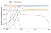Fig. 1. Relative number densities of atomic and ion species with respect to the total density of baryons, as a function of redshift. The computation goes from z = 104 to z = 10. Hydrogen species are represented as full lines, helium as dashed lines, and deuterium as dash-dotted lines. We indicate the recombination redshifts of primordial helium, deuterium and hydrogen nuclei (He2+, He+, then D+ and H+) with vertical dotted line.

HeH⁺ molecule. Helium is the first neutral atom that appeared in the Universe (see Fig. 1). One of the first molecular bonds to be formed is HeH⁺ via radiative association processes¹: He⁺+H→HeH++ν (see Roberge & Dalgarno 1982; Kraemer et al. 1995) and He+H⁺→HeH⁺+ν (see Zygelman et al. 1998). It then mostly contributes to the production of H${}_2^{+}$ via exchange reaction (${\mathrm{HeH}}^{+}+\mathrm{H}\to {\mathrm{H}}_2^{+}+\mathrm{He}$). Schleicher et al. (2008) also showed that this molecule can play a role in the smearing of primordial fluctuations by scattering CMB photons. Thus, helium is an important component to initiate, at the earliest times, the primordial chemistry. Once a large number of helium atoms are formed through the recombination process, charge transfer with ions becomes possible, initiating the formation of the other neutral species. However, HeH⁺ appears to be negligible in the molecular cooling processes.

Molecular hydrogen. Molecular hydrogen cannot form directly by radiative association between two neutral atoms because H₂ does not have a permanent dipole moment. Charge transfer H${}_2^{+}+\mathrm{H}\to {\mathrm{H}}_2+{\mathrm{H}}^{+}$ becomes the only alternative. Once HeH⁺ was formed, this ion became an important source of H${}_2^{+}$ production through the exchange reaction with some neutral H. Then, H${}_2^{+}$ charge transfer with a neutral species led to H₂ molecules. Moreover, as the radiation temperature decreases, H₂ can be formed through H⁻ by radiative attachment H+e⁻→H⁻+γ, followed by associative detachment H⁻+H→H₂+e⁻ (Field 2000). For densities over 10⁸ cm⁻³, H₂ molecule can be effectively formed via three-body reaction H+H+H→H₂+H. However, the baryon density after thermal decoupling is ∼550 cm⁻³, which makes this channel ineffective in the context of a homogeneous Universe. The two major routes of H₂ formation are visible in Fig. 2 through the two jumps at the redshifts z∼1000−500 (H${}_2^{+}$ channel) and z∼150 (H⁻ channel). After the freeze-out of the relative abundances, we found n_rel(H₂) = 2×10⁻⁶ for the H₂ molecule. We notice that H${}_3^{+}$ appeared in the early Universe. However, H${}_3^{+}$ reactions, which are pivotal to the chemistry of dense interstellar clouds (see Oka 1980; Tennyson 1995; Herbst 2000), do not play a significant role in primordial chemistry.

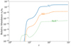Fig. 2. Relative number densities of molecular species with respect to the total density of baryons, as a function of redshift. The computation goes from zi = 104 to zf = 10.

Molecular deuterium. Deuterated-hydrogen molecules have permanent dipole moments, which provide them the capacity to be formed by radiative association (forbidden between two hydrogen atoms). Nevertheless, HD formation is significant when H₂ appeared, as the mechanism of dissociative collision H₂+D⁺→H⁺+HD becomes efficient (see Palla et al. 1995; Stancil & Dalgarno 1998; Signore & Puy 2009). Due to the slight difference between the electronic structure of D and H, H₂ and HD significantly appeared at the same epoch, as shown in Fig. 2. The relative abundance of the HD molecule lies at n_rel(HD) = 6.1×10⁻¹⁰ after the freeze-out.

2.5. Molecular thermal functions

The formation of primordial molecules such as H₂ and HD generates thermal responses due to the excitation of rotational and vibrational levels of molecules. In the range of kinetic and radiation temperature considered, only the rotational levels can be excited. Rotational level populations depend on collisional reactions and radiative processes (CMB absorption or induced and spontaneous emission). Two mechanisms are able to excite or de-excite molecules rotational levels, illustrated in Fig. 3. A molecule can be radiatively excited from a level J to a superior one J′, by absorbing a photon external to the medium (for instance from the radiative background), then become de-excited via a collision with another atom or molecule from the medium. The external photon energy in converted into kinetic energy; hence, we need to consider molecular heating. A molecule can be also excited by a collision from level J to J′, then emit a photon by spontaneous or induced de-excitation to the J level. If the photon is not reabsorbed by the medium, the associated energy is lost and we would be considering molecular cooling.

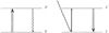Fig. 3. Schematic illustration of the transitions between 2 rotational levels J and J′. Left: Molecule is excited to J′ level by collision (double arrow), then de-excited by photon emission (wavy arrow). Assuming an optically thin medium, the photon is not reabsorbed, and the medium is cooled. Right: Molecule is excited by absorption of a photon (single arrow), then de-excited by collisions. The transition energy injected by the photon is then transmitted to the medium in the form of kinetic energy and the medium is heated.

To express the energy per volume unit that can be gained, Γ_mol (heating), or lost, Λ_mol (cooling), by the medium due to rotational level transitions, we define the thermal molecular function:

$${\mathrm{\Psi }}_{\mathrm{mol}}={\mathrm{\Gamma }}_{\mathrm{mol}}-{\mathrm{\Lambda }}_{\mathrm{mol}}.$$(16)

We detail in Appendices A and B, the computation of the heating and cooling terms, as well as the rotational level populations.

2.5.1. Molecules thermal influence

H₂ is homonuclear, which implies that it does not possess a permanent dipole moment, which strongly diminish its thermal effect. However, as it is the most abundant molecule, the thermal function due to H₂ plays a role in numerous astrophysical medium (Le Bourlot et al. 1999). In the post-recombination context, H₂ contributes to heat the medium. Nevertheless, in Fig. 4, where we compare the thermal channel contributions in T_k evolution, we can see that the influence of H₂ on the background gas temperature (see Eq. (8)) is negligible (as already shown in Puy et al. 1993 and Pfenniger & Puy 2003).

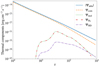Fig. 4. Evolution of cooling and heating components of the gas temperature as a function of redshift, in the homogeneous expanding universe scenario. All the components are described in terms of energy density per second. Ψadia arises from the expansion of the universe. As it is negative (cooling component), we display it as an absolute value. Ψcom is due to Compton coupling between matter and radiation. ${\mathrm{\Psi }}_{\mathrm{mol}}={\mathrm{\Psi }}_{{\mathrm{H}}_2}+{\mathrm{\Psi }}_{\mathrm{HD}}$ corresponds to the thermal contribution of molecules H2 and HD.

Infrared emissivities of HD were computed by Dalgarno & Wright (1972). The existence of a permanent dipole moment and its excitation temperature (21 K compared to 112 K for H₂) give this molecule interesting cooling properties. Puy & Signore (1997) showed, in a collapsing molecular protocloud, HD is the main cooling agent around 200 K, confirmed by Flower et al. (2000) and Nakamura & Umemura (2002). Despite being by far less abundant than H₂, the HD molecule can still provide a considerable thermal contribution at the lowest temperatures, around T_k<200 K because of its permanent dipole (Puy et al. 1993; Galli & Palla 1998; Stancil et al. 1998). However, as H₂, HD cooling does not play a role in the evolution of the gas temperature in a homogeneous expanding universe (Flower 2000; Galli & Palla 1998, 2002). Thus, the molecular thermal function, Ψ_mol, is negligible in the thermochemistry of the homogeneous Universe. We will see its importance in a scenario of gravitational collapse in Sect. 4.

3. 21 cm line implementation

The hyperfine transition line of atomic hydrogen, in the ground state, arises due to the interaction between the electron and proton spins. In the excited triplet state, the spins are parallel, whereas the spins in the ground (singlet) state are antiparallel. The 21 cm line is a forbidden line for which the probability for a spontaneous 1⟶0 transition is given by the Einstein coefficient A₁₀ = 2.85×10⁻¹⁵ s⁻¹. 21 cm signal observable quantity is the differential brightness temperature, which can be expressed as (see e.g., Madau et al. 1997)

$$\delta T_b\approx \frac{3h{c}^3}{32\pi }\frac{A_{10}}{k_B{\nu }_{10}^2}\frac{{\overline{n}}_{\mathrm{HI}}(1+{\delta }_b)}{(1+z)H(z)\left(1+\frac{1+z}{H(z)}\frac{\mathrm{d}{v}_{||}}{\mathrm{d}{r}_{||}}\right)}\left(1-\frac{T_{\gamma }}{T_s}\right),$$(17)

where ν₁₀ = 1420.406 MHz is the 21 cm line rest frequency, ${\overline{n}}_{\mathrm{HI}}$ is the mean neutral hydrogen number density, and δ_b is the relative baryon density perturbation. H(z) is the Hubble rate, and dv_||/dr_|| is the gradient of line of sight peculiar velocity, describing the relative motion of the gas with respect to the Hubble flow. Lastly, T_γ is the radio background temperature, which we set as the CMB one, and T_s is the spin temperature defined from the ratio between the hyperfine population levels.

Hydrogen atoms can be excited by various processes: the absorption and stimulated emission of photons from the CMB redshifted at the 21 cm wavelength, collisions with other hydrogen atoms, free electrons and protons, and Lyman-α radiation from astrophysical sources through Wouthuysen-Field effect (Wouthuysen 1952; Field 1958). During the dark ages, before the formation of the first stars, only the first two mechanisms compete in the excitation of the hyperfine level. In thermal equilibrium, the spin temperature can be written:

$$T_s^{-1}=\frac{T_{\gamma }^{-1}+x_c{T}_k^{-1}}{1+x_c}·$$(18)

x_c is the total coupling coefficient for collisions given by the expression:

$$x_c=\frac{\left(C_H+C_e+C_p\right)}{A_{10}}\frac{T_{10}}{T_{\gamma }},$$(19)

where T₁₀=hν₁₀/k_b is the equivalent temperature of energy splitting between the two hyperfine levels. C_H, C_e, and C_p are the de-excitation rates of the triplet due to collisions with neutral hydrogen, electrons, and protons. The collision term for each i interacting species can be written as $C_i=n_i{\kappa }_{10}^i(T_k)$, where ${\kappa }_{10}^i$ is the effective single-atom rate coefficient for the transition 1-0 from collisions with that species. These rate coefficients are obtained through quantum mechanics computation for collisions with other hydrogen atoms (Zygelman 2005), with free electrons (Furlanetto & Furlanetto 2007a), and with protons (Furlanetto & Furlanetto 2007b).

In the context of homogeneous expanding universe, the brightness temperature of Eq. (17) can be approximated as

$$\delta T_b\simeq \frac{3h{c}^3}{32\pi }\frac{A_{10}}{k_B{\nu }_{10}^2}\frac{n_{\mathrm{HI}}}{H(z)(1+z)}\left(1-\frac{T_{\gamma }}{T_s}\right),$$(20)

$$\simeq 27x_{\mathrm{HI}}\left(\frac{{\mathrm{\Omega }}_b{h}^2}{0.023}\right)\sqrt{\frac{0.15}{{\mathrm{\Omega }}_m{h}^2}\frac{1+z}{10}}\left(1-\frac{T_{\gamma }}{T_s}\right).$$(21)

As the universe is considered homogeneous, we only keep the mean hydrogen density ${\overline{n}}_{\mathrm{HI}}$, and set δ_b = 0. Moreover, we consider an average peculiar velocity equal to zero. The second expression explicits the dependence of the 21 cm signal to cosmological parameters Ω_b and Ω_m, the baryon and matter energy density fraction today, and h, the Hubble parameter in units of 100 km/s/Mpc. Lastly, x_HI is the hydrogen neutral fraction. We show in Fig. 5 (top), the evolution of spin, radiation and kinetic temperatures. The behavior of the spin temperature can be separated in three distinct epochs that determine the observability of the brightness temperature, which is visible in the bottom panel of Fig. 5. These epochs are described as follows.

• Before matter-radiation decoupling, the spin temperature is coupled to the CMB temperature (T_s=T_γ). Differential brightness temperature, δT_b, remains at zero.

• Around z∼z_dec,1% (defined as the redshift at which T_k(z_dec,1%) = 99%T_γ(z_dec,1%)), matter and radiation temperatures are progressively decoupling. The Universe is dense enough for the collision mechanism to dominate in the 21 cm signal production. The spin temperature is thermalized to the gas temperature, T_s→T_k, and the brightness temperature reaches a minimum of δT_b∼−44 mK at z(δT_b,min≈89).

• Due to the expansion of the universe, the baryons get more and more diluted and the collision mechanism progressively becomes ineffective. The spin temperature relaxes to the CMB temperature, T_s→T_γ, which brings δT_b back to zero.

This section has served to present the functioning of CHEMFAST within the known framework of an expanding homogeneous universe. The code can be used to solve a system of stiff coupled differential equations in order to obtain the evolution of the abundance of chemical species based on a network of reactions. The code can also be used to calculate the thermal influence of molecules on temperature through the excitation of their rotational levels. In a homogeneous expanding universe, we can see that this effect is negligible. Finally, by following the thermal history of the universe and the chemical reactions, we can estimate the intensity of the global 21 cm signal due to arising from collisional coupling. The 21 cm global signal computed with CHEMFAST is in accordance with the state-of-the-art literature (see e.g., Furlanetto et al. 2006; Pritchard & Loeb 2012).

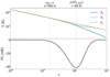Fig. 5. Top: Evolution of kinetic gas temperature, Tk (blue solid line), radiation temperature, Tγ (dashed green line), and 21 cm spin temperature, Ts (orange dash-dotted line), as a function of redshift. Bottom: Evolution of the global 21 cm differential brightness temperature as a function of redshift. At zdec,1% (Tk = 99% Tγ), thermal decoupling starts to be effective. At z(δTb,min), δTb reaches its lowest point, corresponding to the maximum absorption during the dark ages.

4. Dynamics of collapsing clouds and 21 cm hydrogen line emission

In the context of homogeneous expansion seen in the first part, the thermal influence of H₂ and HD molecules on the gas temperature is negligible, due to their very low mean abundances. Their contribution is completely drowned out by the adiabatic cooling of the matter-radiation thermal coupling associated with Compton scattering. However, we know that the universe is actually not homogeneous, but exhibited small primordial density fluctuations, which became seeds for the formation of structures.

When a density perturbation grows enough due to gravity in order to reach a density contrast comparable to unity, it can no longer be described by the linear theory of perturbations. We must then consider a model to follow its evolution until a potential collapse. Molecules in overdensities are known to cool the gas via the excitation of their rotational and vibrational levels and permitting the further gravitational collapse of the gas, thereby setting up the right conditions for the formation of the first structures.

In this section we focus on the evolution of an individual overdensity. We implement a collapse model in CHEMFAST by modifying the equations of dynamics. Our goal is then to estimate the 21 cm signal from the collapsing overdensity under the influence of molecular cooling.

4.1. Model of collapsing cloud

We consider a spherical pressure-supported collapse model with basic hypothesis. The model we use is based on the work of Lahav (1986), extended by Puy & Signore (1996). Unlike the free-fall model, the spherical collapse we consider cannot be solved analytically and requires a numerical resolution.

We assume that the overdense region we follow is isothermal, spherical, and without rotation. We also assume the matter density to be constant inside the overdense region. This matter sphere, at first following the expansion of the universe, will progressively slow down with respect to the background, due to the density excess, until the point when it drops out of expansion, and starts to collapse back on itself. In the range of redshift we consider, the universe is fully dominated by matter, and we can assume a linear t^2/3 growth of the fluctuations with the expansion of the Universe. Hence, we consider a spectrum of isothermal perturbations, that are described by the spectrum (Gott & Rees 1975):

$$\frac{\delta \rho }{\overline{\rho }}={\left(\frac{M}{M_0}\right)}^{-1/3}(1+z{)}^{-1},$$(22)

where the mass M of the overdense region is normalized to M₀, defined as a characteristic mass-scale of M₀ = 10¹⁵ M_⊙, which is the typical mass of large galaxy clusters today, also used in Lahav (1986).

4.2. Equations

As in Sect. 2, here we solve a set of differential equations, this time for a collapsing overdense region.

Baryon number density. The matter conservation inside the cloud gives:

$$\frac{\mathrm{d}{n}_b}{\mathrm{d}t}=-3\frac{n_b}{r}{v}_r+{\displaystyle \sum _{\xi }}{\left(\frac{\mathrm{d}{n}_{\xi }}{\mathrm{d}t}\right)}_{\mathrm{chem}},\hspace{0.5em}\mathrm{with}\hspace{0.5em}{v}_r=\frac{\mathrm{d}r}{\mathrm{d}t}.$$(23)

The equation is similar to the expansion case of Sect. 2, the scale factor, a, is simply replaced by the radius of the cloud, r. The last term in the right-hand side of the equation is the contribution from chemical reactions.

Species densities. Similarly, for each chemical component ξ we have

$$\frac{\mathrm{d}{n}_{\xi }}{\mathrm{d}t}=-3\frac{n_{\xi }}{r}{v}_r+{\left(\frac{\mathrm{d}{n}_{\xi }}{\mathrm{d}t}\right)}_{\mathrm{chem}}.$$(24)

Temperatures. The radiation temperature evolves just like in the homogeneous case, with the expansion of the universe:

$$\frac{\mathrm{d}{T}_{\gamma }}{\mathrm{d}t}=-H(t)T_{\gamma }.$$(25)

The kinetic gas temperature, under the assumption of perfect gas, can be computed as:

$$\frac{\mathrm{d}{T}_k}{\mathrm{d}t}=\frac{2}{3n_b{k}_B}\left({\mathrm{\Psi }}_{\mathrm{grav}}+{\mathrm{\Psi }}_{\mathrm{mol}}+{\mathrm{\Psi }}_{\mathrm{com}}\right).$$(26)

${\mathrm{\Psi }}_{\mathrm{grav}}=-3n_b{k}_B{T}_k\frac{v_r}{r}$ accounts for the density variation arising from the gravitational collapse, Ψ_com describes the Compton coupling between matter and radiation (see Eq. (10)), and Ψ_mol expresses the thermal influence of molecules on the gas temperature through the excitation of their rotational levels (see Appendix A).

Radius and velocity of collapse. Starting from the energy balance:

$$E=-\frac{3}{5}\frac{{\mathit{GM}}^2}{r}+\frac{3}{10}M{v}_r^2+\frac{3}{2}{N}_b{k}_b{T}_k,$$(27)

where the first term corresponds to the potential energy in a spherical system with a central potential. The second one accounts for the associated kinetic energy, and the last one for the internal energy. Then, N_b the total number of baryons in the cloud.

We inject the temperature into Eq. (26), expressing the energy variation in the system as $\frac{\mathrm{d}E}{\mathrm{d}t}=r^3({\mathrm{\Psi }}_{\mathrm{com}}+{\mathrm{\Psi }}_{\mathrm{mol}})$, and use $M=N_b{\mu }_b{m}_H\frac{{\mathrm{\Omega }}_m}{{\mathrm{\Omega }}_b}$² to obtain

$$a_r=-\frac{\mathit{GM}}{r^2}+\frac{5k_b{T}_k}{\mu m_H}\frac{1}{r}\frac{{\mathrm{\Omega }}_b}{{\mathrm{\Omega }}_m}\hspace{0.5em}\hspace{0.5em}\mathrm{with}\hspace{0.5em}\hspace{0.5em}{a}_r=\frac{\mathrm{d}{v}_r}{\mathrm{d}t}·$$(28)

4.3. Initial conditions

Considering a single cloud of mass, M, we follow the collapse starting from the turnaround point, when the gravity takes over the expansion and the perturbation starts to increase in density, as it was only diluting slower than the background before this moment. In a spherical collapse model, an overdense region reaches the turnaround point when the density contrast reaches ${\left(\frac{3\pi }{4}\right)}^2$ (Padmanabhan 2002; Peebles 1980).

Hence, the baryon number density at turnaround is expressed by

$$n_{b,\mathit{ta}}={\left(\frac{3\pi }{4}\right)}^2{\overline{n}}_b(z_{\mathit{ta}}).$$(29)

Where ${\overline{n}}_b(z_{\mathit{ta}})$ is the background baryon number density at turn-around redshift, z_ta.

Following the approach of Gunn et al. (1972) and Lahav (1986), we compute the redshift of turn-around for a given mass:

$$1+z_{\mathit{ta}}={\left(\frac{3\pi }{4}\right)}^{-2/3}{\left(\frac{M}{M_0}\right)}^{-1/3}.$$(30)

This is the redshift at which we start to follow the collapse in CHEMFAST. It is only dependent of the mass, M, of the cloud.

The radius of the overdense region is directly derived from the density

$$r_{\mathit{ta}}={\left(\frac{3M}{4\pi {\rho }_{b,\mathit{ta}}}\right)}^{1/3},$$(31)

with ρ_b,ta=μ_bm_H n_b,ta. The collapse velocity v_ta at turn-around is by definition set at zero:

$$v_{\mathit{ta}}=\frac{\mathrm{d}{r}_{\mathit{ta}}}{\mathrm{d}t}=0.$$(32)

For the gas temperature, the computation is less evident. If the gas and radiation temperature were fully decoupled, we could consider the adiabatic gas temperature evolves as T_k(z)∝ρ_b(z)^2/3. Then, the gas temperature inside an overdensity at turnaround redshift could be written

$$T_{k,\mathit{ta}}^{\mathrm{adia}}={\left(\frac{3\pi }{4}\right)}^{4/3}{\overline{T}}_k(z_{\mathit{ta}}),$$(33)

where the adia label refers to adiabatic, in the sense that the gas temperature only changes due tot the expansion or compression of its environment, without any exchange of heat. However, as we will see, our model can provide very high redshift of turn-around, depending on the chosen mass. As a consequence, the gas temperature does not fully evolve adiabatically, and the Compton scattering between free electrons and photons can still be efficient at the turn-around redshifts. Choosing $T_{k,\mathit{ta}}^{\mathrm{adia}}$ would mean ignoring the effect of Compton scattering in the period preceding the turnaround. We therefore need to estimate the temperature at turn-around, which lies in the range $\left[{\overline{T}}_k(z_{\mathit{ta}}),{\left(\frac{3\pi }{4}\right)}^{4/3}{\overline{T}}_k(z_{\mathit{ta}})\right]$, accounting for the residual Compton coupling. We chose the turnaround temperature empirically, such that the Compton thermal channel, Ψ_com, is steady in the very first moments of collapse at the beginning of the run. Actually, we have checked that this detail does not significantly impact the behavior of T_k during the rest of the collapse. It does, however, help to avoid non-physical behavior³ in the very first moments of the collapse.

To summarize, our model takes the mass of the overdense region as the only free parameter, from which all the initial conditions are derived. For a given mass, we ran CHEMFAST a first time in expansion mode up to the turnaround redshift and extracted the background values of the species abundances, baryon density, and temperatures. These data were then used to compute the initial conditions in the collapse setup.

5. Results

5.1. Thermal evolution of 10⁸ M_⊙ collapsing cloud

We focus on the analysis of a 10⁸ M_⊙ collapsing overdensity, which corresponds to the order of magnitude expected for “massive minihalos”, the least massive halos that are expected to be able to host star formation (see e.g., Tegmark et al. (1997), Yoshida et al. (2003), Glover (2005), Haiman & Bryan (2006), Trenti & Stiavelli (2009), Greif (2015) for discussions on the formation of the first structures). In our model, this overdensity reaches its redshift of turnaround at z_ta = 93, with a temperature $T_{k,\mathit{ta}}=2.1·{\overline{T}}_k(z_{\mathit{ta}})$. We first discuss the evolution of the gas temperature from its different thermal channels and then propose an estimate of the 21 cm line arising from the collapsing overdensity.

For all the following figures, we display the evolution of the quantities as a function of the time to collapse. Defining the turnaround time:

$$t_{\mathit{ta}}=\sqrt{\frac{3\pi }{32G{\rho }_{\mathit{ta}}}},$$(34)

the time of re-collapse can be expressed as t_coll = 2t_ta (Lahav 1986). We normalized time in the figures to evolve between 0 and 1.

In Fig. 6, we follow the intensity of all the thermal channels acting on the gas temperature within the cloud (see Eq. (26)). The heating due to gravitational contraction, Ψ_grav (solid blue line), gets stronger as the radius of the halo decreases and the collapse velocity increases; Ψ_com (dashed curve) arises from the Compton coupling between matter and radiation. Since our initial conditions provide a gas temperature in the halo above the background radiation temperature, the Compton interaction tends to cool the gas temperature towards the radiation temperature, which explains why it presents a negative contribution. The Compton coupling dominates over the other contributions in the first instants and decreases as the collapse progresses. It eventually becomes negligible.

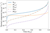Fig. 6. Evolution of cooling and heating components of the gas temperature in a 108 M⊙ collapsing cloud as a function of time, normalized by tcoll. All the components are described in terms of energy density per second. Ψgrav arises from to gravitational collapse of the gas; Ψcom is due to Compton coupling. Finally, ${\mathrm{\Psi }}_{\mathrm{mol}}={\mathrm{\Psi }}_{{\mathrm{H}}_2}+{\mathrm{\Psi }}_{\mathrm{HD}}$ corresponds to the thermal contribution of molecules H2 and HD. The negative components Ψcom, Ψmol, ${\mathrm{\Psi }}_{{\mathrm{H}}_2}$, and ΨHD are displayed as absolute values.

The Ψ_mol term (dotted curve) represents the molecular thermal function summing over the contributions from the two most important molecules ${\mathrm{\Psi }}_{{\mathrm{H}}_2}$ and Ψ_HD. Furthermore, Ψ_mol is almost completely driven by H₂ molecule. The HD contribution becomes important for lower temperatures than the one we are interested in (<200 K), it is negligible in the case we are studying (McGreer & Bryan 2008). In Fig. 6, Ψ_mol contributes to cool the gas. Initially negligible, its importance increases sharply as the density of the molecules increases and the gas temperature grows, until it becomes significant and even dominates the other thermal channels at the end of the collapse. Compared to the expansion scenario, the molecular thermal function has a strong influence on the gas temperature.

We display the evolution of the radiation and gas temperatures inside the 10⁸ M_⊙ collapsing overdensity in Fig. 7 (top panel). The radiation temperature evolves exactly in the same way as in the background, and is shown for comparison. The evolution of the gas temperature can be divided in several stages:

• During the very first moments of the collapse, Compton coupling is the dominant thermal mechanism and tends to bring T_k (blue solid line) to T_γ (green dashed line) acting against gravitational contraction. As a result, the gas temperature inside the overdensity slightly decreases. This stage holds for a very short time; hence, the decrease is not visible in the figure.

• Heating due to the gravitational collapse rapidly dominates over the Compton coupling, starting from t = 0.06t_coll. From this moment, the gas temperature inside the cloud grows drastically, under the influence of gravity.

• Molecular cooling rapidly becomes more important due to the increasing gas temperature and H₂ density inside the cloud. This thermal channel dominates, starting from t = 0.89t_coll, the molecular thermal function cools the medium more than it heats up by gravitational contraction. The gas temperature inside the cloud decreases despite the ongoing collapse.

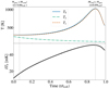Fig. 7. Top: Evolution of radiation temperature, Tγ (dash-dotted line), gas temperature, Tk (solid line) and 21 cm spin temperature, Ts (dotted line) for a collapsing 108 M⊙ cloud, as a function of the time to collapse. We highlight on top of the figure the times when the dominant thermal channel changes. Bottom: Evolution of the associated 21 cm brightness temperature from a collapsing 108 M⊙ cloud.

5.2. 21 cm line emission from collapsing halo

At the top of Fig. 7, we can see the spin temperature, T_s (dashed line), closely follows gas temperature, T_k, throughout the collapse. Looking again at the spin temperature (Eq. (18)), we can explain it by the following arguments. We are in a collapse scenario, where the matter number density is increased up to a factor ∼177 compared to the background, at the end of the collapse. Therefore, the collisional coupling is important and dominates the 21 cm line production.

The differential brightness temperature, δT_b, is positive, meaning that the signal presents an emission feature, different from the global signal absorption feature from the expansion scenario. Throughout the collapse, T_s is always greater than radiation temperature, T_γ. Therefore, the term $\left(1-\frac{T_{\gamma }}{T_s}\right)$ in Eq. (21) stays between 0 and 1. Moreover, we observe in δT_b the same type behavior than T_k, with a turnover caused by molecular cooling. Indeed, since the spin temperature completely follows T_k, it is sensitive to the same thermal processes, transmitted to δT_b. We can note that, even without the activation of molecular cooling, δT_b would eventually saturate and reach a maximum limit when T_s≫T_γ. In this regime, the dependence on T_s in Eq. (21) would become unimportant.

We adopted the Eq. (21) for the computation of the 21 cm differential brightness temperature. By doing so, we made several approximations, to which we dedicate the following discussion. Firstly, we assumed a zero peculiar velocity for the halo. This choice is not problematic by itself, but it should be noted that it is arbitrary. When studying a whole population of halos, we have to take into account the effects of peculiar velocities, which induce an enhancement of the fluctuations at all scales (Bharadwaj & Ali 2004; Barkana & Loeb 2005).

Equation (21) also implies two major approximations for calculating the 21 cm signal from a halo. The supposition that the optical depth is thin can no longer technically hold in a halo. For an accurate calculation, it would be more appropriate to consider a density profile (such as a truncated isothermal sphere used in Iliev et al. 2002, or a Moore profile used in Furugori et al. 2020) for the halo; instead of a homogeneous density as we have done. The optical depth would then vary as a function of radius (maximum at the center of the halo where the maximum amount of matter is traversed) and the brightness temperature shall be integrated over the surface of the halo. The other approximation we make is to assume the 21 cm line profile as a Dirac function. A more appropriate approximation, such as a thermal-Doppler-broadened line profile, would allow the velocity dispersion of particles within the halo to be taken into account.

However, accounting for the variable optical depth and the Doppler broadening would require us to get rid of the assumption of homogeneous density and temperature in the halo; it could also strongly modify the 21 cm signal. The results we show are in that sense approximations, presenting our approach, and we leave the improvement of the collapse model to a future work.

5.3. Thermal evolution of a range of halo masses

After focusing on the physics at work in a 10⁸ M_⊙ collapsing halo, we present the temperatures evolution for a whole range of different masses in Fig. 8 and display their associated turnaround redshifts and gas temperature in Table 2. Several masses are shown in the same figure as a function of their time to collapse in order to easily compare them. However, it is important to bear in mind that these collapses take place at different redshifts, which are correlated with the initial mass.

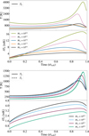Fig. 8. Top: Evolution of gas temperature, Tk (solid lines), for clouds of mass between 106.0 and 108.0 M⊙, as a function of the time to collapse (top). On the bottom of this plot are displayed the 21 cm differential brightness temperatures. Bottom: Same as the top panel, for masses between 108.0 and 108.8 M⊙, also displaying the 21 cm spin temperature Ts (dotted lines).

In the top panel of Fig. 8, we show the temperatures evolution for masses between 10⁶ and 10⁸ M_⊙. The gas temperature presents the same general behavior for all the masses: a growth provoked by the contraction of the clouds, followed by a decline in the last moments of the collapse, due to the molecular cooling. However, the fall in T_k occurs at different moments of the collapse depending on the mass. It happens later for the smaller masses, such as 10⁶ M_⊙, resulting in a higher maximal gas temperature, and 21 cm brightness temperature.

On the other hand, we notice an inversion of this behavior starting from masses > 10^7.0 M_⊙. We observe that the maximum gas temperature increases again and the moment of collapse at which the maximum temperature is reached is delayed.

Looking at the top of Fig. 9, where is plotted the ratio between Ψ_mol and Ψ_grav, we observe that above 10⁷ M_⊙, the more we increase the mass of the cloud, the later the molecular cooling dominates. This effect can be understood by looking at the number density of H₂ inside the halos, presented in the bottom panel of Fig. 9. We can expect a higher overall baryon density in the halos of smaller mass, as they are the first ones to form. The density contrast between the overdense region and the background is similar for all halos, so the one forming when the background is denser are also expected to show a higher density. However, the H₂ density directly depends on the presence of the species leading to its formation, H${}_2^{+}$ via charge transfer reaction ${\mathrm{H}}_2^{+}+\mathrm{H}\to {\mathrm{H}}_2+\mathrm{H}$, and H⁻ via associative detachment H⁻+H→H₂+e⁻. Finally, H⁻ is actually rapidly destroyed by CMB photons when forming at very high redshift, before it would be able to contribute to H₂ formation.

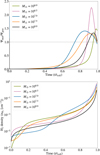Fig. 9. Top: Evolution of ratio between Ψmol and Ψgrav thermal channels, arising from molecular excitation and gravitational contraction respectively, for clouds between 106.0 and 108.0 M⊙, as a function of the time to collapse. Bottom: H2 number density evolution as a function of the time to collapse, for clouds between 106.0 and 108.0 M⊙.

For the lowest masses (e.g., 10⁶ M_⊙, which has a turn-around redshift of z_ta = 436 in our model), despite a high overall density in the cloud, the formation of H₂ molecules by the H⁻ channel is strongly suppressed. Up to ∼10⁷ M_⊙ (z_ta = 202), the H⁻ are progressively less destroyed, allowing more H₂ to be formed and resulting in stronger molecular cooling. In the homogeneous universe (see Fig. 2), the growth of the H₂ population via H⁻ takes place around z = 150, when the temperature of the photons decreases enough such that it does not allow them to destroy H⁻ anymore, letting it maximally convert into H₂. However, as the >10⁷ M_⊙ halos form later and later, even if the H⁻ population is not suppressed, the baryons density (and therefore the H₂ density) progressively decreases, explaining the gradual decline of molecular cooling.

Interestingly, the 21 cm brightness temperature does not present the same behavior and the highest maximum δT_b is still reached in the lightest halos. The reason lies in the redshift dependence of the signal, which is not visible in the figure, but is explicit in Eq. (21). The collapses of the largest masses occur too late and the gas temperature increase is not enough to overcome the decline in redshift, even though T_s is still strongly coupled to T_k via collisions, as can be seen in the bottom panel of Fig. 8.

6. Discussion and perspectives

We explored the evolution of species abundances in detail during and after successive recombinations. To do so, we improved the code CHEMFAST, which solves a system of stiff coupled differential equations. Part of the system describes the dynamics (density, baryon, and radiation temperatures) and another is dedicated to describing the network of collisional, electronic, and photo-processes between the species. Particular attention has been paid to tracking the molecular abundances.

We first applied CHEMFAST to the simple expanding homogeneous universe framework. We computed the successive recombinations of He²⁺, He⁺, H⁺, and D⁺, as well as the relative abundances of all the atoms, ions, and molecules contributing to the reaction network. We also computed the thermal influence of molecules through the excitation of their rotational levels. Furthermore, we implemented the 21 cm differential brightness temperature global signal computation during the dark ages, arising from collisional excitation. It presents an absorption peak with an intensity of -40 mK at z = 89. This result is largely corroborated by the literature (e.g., Furlanetto et al. 2006; Pritchard & Loeb 2012) and validates the effectiveness of our code.

In a second study, our goal was to investigate the 21 cm signal evolution in a new context and to assess how it could be distinguished from the sky-averaged global signal. To this end, we flexibly integrated a new set of dynamical equations into our abundance calculation code CHEMFAST, to follow the collapse of an overdense region. We based our work on a spherical collapse model developed by Lahav (1986), taking into account the pressure forces, with the cloud mass as the only free parameter. We followed the collapse of a typical cloud of 10⁸ M_⊙, expected to be able to host the formation of the first galaxies. Within the collapse, molecules are present in much greater density than in the homogeneous case. Calculating the excitation of the rotational levels for the H₂ and HD molecules shows us that they have a strong thermal impact on the cloud's gas temperature. At this point, the contribution becomes dominant and takes over the gravitational heating in the last moments of the collapse, leading to a cooling of the gas.

Finally, we computed the 21 cm line brightness temperature within the collapsing cloud. The signal shows a very different signature compared to the global signal of the dark ages. It presents an emission feature and is also affected by molecular cooling, in the same way as the gas temperature to which the brightness temperature is coupled via collisions. We also present the thermal evolution for overdense regions of 10⁶ to 10^8.8 M_⊙. The strongest 21 cm signals are expected from the halos of the lowest masses, which have lower H₂ abundances, due to the suppression of the H⁻ formation channel by CMB radiation. These halos therefore exhibit less efficient molecular cooling. The intensity of molecular cooling increases progressively with the halo masses until redshifts z∼150 at which H⁻ is no longer destroyed. Halos whose formation begins after this redshift see a decline in molecular cooling, due to their lower density. Despite a higher T_k, this pattern is not followed by the 21 cm brightness temperature because of its redshift dependence. The H₂ chemistry is not trivial, however, and further investigation would be required to understand the H₂ density evolution in collapse context, depending on the initial mass. We plan to conduct this investigation in a future work.

These particular signatures of the 21 cm signal are promising with respect to probing the thermal history inside halos. They could also present an observational interest at the smallest scales of the 21 cm power spectrum in the context of the forthcoming lunar-based observations of the dark ages. One way to estimate this impact would be to compute the brightness temperature arising from a whole halo population, by associating our single halo results to the computation of a halo mass function (Lukić et al. 2007; Murray et al. 2013). However, the particularly high turnaround redshifts of our collapse model make the determination of the halo mass function particularly challenging.

Indeed, our model predicts cloud formation at particularly high redshifts, compared to what is currently proposed in the literature (e.g., Trenti & Stiavelli 2009; Glover 2012; Greif 2015). State-of-the-art halo formation models start at redshifts of z∼30 for the halos of the lowest mass, which are still allow the gas to collapse (∼10⁵−10⁶ M_⊙). Similar ranges are found by studies of 21 cm signal predictions from halos Iliev et al. (2002), Furugori et al. (2020), Novosyadlyj et al. (2024), which makes it difficult to make comparisons with them, as our hypotheses are very different. This discrepancy can be explained by the simplicity of the model we have chosen. Furthermore, we have seen that the assumption of homogeneous density and temperature inside the cloud could prove problematic for the study of the 21 cm signal. We intend to study other collapse models with CHEMFAST in future work and include the density and temperature profiles in our modeling. We also plan to integrate elliptical geometries, which are more consistent with collapse simulations.

Lastly, molecular cooling can induce the development of thermal instabilities. These effects were first studied by Parker (1953), followed by Field (1965), and later Balbus (1986), who derived instability criteria, leading to a growth of the perturbations in the gas. It is now understood that these thermal instabilities play an important role in the fragmentation of halos and the formation of the first stars (Safranek-Shrader et al. 2010; Yoshida et al. 2006; Bromm 2013; Glover 2012; Greif et al. 2013). The aim of our simple model has been to highlight the crucial thermal influence of molecules on the thermal history and 21 cm signal, but it does not allow us to explore the evolution of thermal instabilities in depth. We would then have to turn to adaptive mesh refining (AMR) type simulations, such as the ENZO (Bryan et al. 2014) or RAMSES (Teyssier 2002) codes. This type of approach makes it possible to spatially monitor instabilities that can lead to fragmentation within the structures (Tang & Chen 2024).

Acknowledgments

We thank Alice Faure for her support in the code optimization. We also thank Daniel Pfenniger and Benoît Sémelin for helpful discussions. These results have been made possible thanks to LUPM's cloud computing infrastructure, founded by PHONE project - Occitanie Regions, Ocevu labex, and France-Grilles.

References

Appendix A: Details on molecular thermal function

In this appendix, we detail the heating and cooling terms composing the molecular thermal function:

$${\mathrm{\Psi }}_{\mathrm{mol}}={\mathrm{\Gamma }}_{\mathrm{mol}}-{\mathrm{\Lambda }}_{\mathrm{mol}}.$$(A.1)

A.1. Molecular heating

The collisional de-excitation probability expresses the ratio between the collisional de-excitation rate and the total de-excitation rate, which includes collisions, as well as induced and spontaneous emissions, as follows:

$$P_{J\prime ,J}^c=\frac{n_{\xi }{X}_{J\prime }{k}_{J\prime ,J}^{\xi }}{n_{\xi }{X}_{J\prime }{k}_{J\prime ,J}^{\xi }+X_{J\prime }{A}_{J\prime ,J}+X_{J\prime }{B}_{J\prime ,J}{\rho }_{J\prime ,J}}.$$(A.2)

Here, n_ξ is the numerical density of the collision partner species, ξ, and X_J′ is the population fraction of molecule in the rotational level J′. Then, $k_{J\prime ,J}^{\xi }$ is the collision rate of this reaction, while A_J′,J and B_J′,J are the Einstein coefficients for spontaneous and induced emission, respectively, and ρ_J′,J is the radiation energy density. Each term of the sum is the de-excitation term associated to one of the three mentioned processes.

Taking the product between the molecule density at J level,n_molX_J, the induced radiative excitation probability, B_J,J′ρ_J,J′, the collisional de-excitation probability, $P_{J\prime ,J}^c$, and the energy difference between the two levels, Δϵ_J′,J=ϵ_J′−ϵJ, we can compute the energy gained by the medium per unit of volume and time through molecular thermal influence:

$${\mathrm{\Gamma }}_{\mathrm{mol}}={\displaystyle \sum _J}{\displaystyle \sum _{J\prime }}{n}_{\mathrm{mol}}{X}_J{B}_{J,J\prime }{\rho }_{J,J\prime }{P}_{J\prime ,J}^c\mathrm{\Delta }{ϵ}_{J\prime ,J}.$$(A.3)

We summed over all the J′ levels reachable by excitation as well as over J to take into account the contribution from all the rotational levels.

The energy of a rotational level, J, can be computed as:

$${ϵ}_J=h\mathit{BJ}(J+1)\hspace{0.5em}\mathrm{where}\hspace{0.5em}B\hspace{0.5em}\mathrm{is}\hspace{0.5em}\mathrm{the}\hspace{0.5em}\mathrm{rotation}\hspace{0.5em}\mathrm{constant}\hspace{0.5em}B=\frac{h}{8{\pi }^2\mathit{cI}},$$(A.4)

with I the momentum of inertia.

A.2. Molecular cooling

By analogy, we first compute the radiative de-excitation probability:

$$P_{J\prime ,J}^r=\frac{X_{J\prime }{A}_{J\prime ,J}+X_{J\prime }{B}_{J\prime ,J}{\rho }_{J\prime ,J}}{n_{\xi }{X}_{J\prime }{k}_{J\prime ,J}^{\xi }+X_{J\prime }{A}_{J\prime ,J}+X_{J\prime }{B}_{J\prime ,J}{\rho }_{J\prime ,J}},$$(A.5)

which is the ratio of both induced and spontaneous radiative de-excitation rates, to the total one.

We change the radiative excitation probability from Eq. A.3 to the collisional excitation probability with species ξ: $n_{\xi }{k}_{J,J\prime }^{\xi }$ and change the collisional de-excitation probability to the radiative one (Eq. A.5). We can then compute the energy lost by the medium per unit of volume and time through molecular thermal influence:

$${\mathrm{\Lambda }}_{\mathrm{mol}}={\displaystyle \sum _J}{\displaystyle \sum _{J\prime }}{n}_{\mathrm{mol}}{n}_{\xi }{k}_{J,J\prime }^{\xi }{X}_J{P}_{J\prime ,J}^r\mathrm{\Delta }{ϵ}_{J\prime ,J}?.$$(A.6)

Appendix B: Molecular rotational levels

This appendix is mainly inspired by Puy & Signore (1997) and Vonlanthen (2009). The aim is to compute, X_J, the population fraction of molecules in each rotational level, J.

B.1. Einstein coefficients

Let us assume a container inside which there is a radiation field of density ρ(ν)dν and molecules capable of passing from a rotational level J to a higher level J′ by the absorption of a photon whose energy h_Pν_JJ′ corresponds to the energy difference between the two levels (radiative excitation) or by collision (collisional excitation). De-excitation can also be collisional or radiative (spontaneous or induced).

There are three radiative processes: spontaneous emission, induced emission, and absorption. The Einstein coefficients A_J′J and B_JJ′ are defined as follows:

• Spontaneous emission: the probability of spontaneous emission A_J′J is the probability that a molecule in the rotational state J′ spontaneously emits a photon of energy h_Pν_JJ′ corresponding to the transition from J′ to J.

• Induced emission: The probability of induced emission is defined by the probability that the atom passes from J′ to J when it is subjected to induced radiation with a frequency between ν_J′ and ν_J′+dν. This probability is denoted B_J′Jρ(ν).

• Absorption: absorption occurs when a molecule in the J state, exposed to isotropic radiation of density ρ(ν)dν and frequency between ν_J′ and ν_J′+dν, absorbs a photon of energy h_Pν_JJ′ and changes to the J′ state. We write the probability of absorption B_JJ′ρ(ν).

If we write I the moment of inertia of a molecule, then the energy of the rotational level J is given by Cohen-Tannoudji et al. (1973) and Kutner (1984):

$${ϵ}_J=\frac{J(J+1)h_{\mathrm{P}}^2}{8{\pi }^{2}I},$$(B.1)

with h_P the Planck constant. We can rewrite this as:

$${ϵ}_J=h_{\mathrm{P}}\mathit{BJ}(J+1),$$(B.2)

where B=h_P/8π²I is called the molecule's rotation constant. We can see that the more massive a molecule is, the greater its moment of inertia will be, and therefore the smaller its rotation constant will be. Transition frequencies are obtained by taking the energy differences between two levels and dividing by h_P. For dipole molecules, transitions obey the rule $\left|\mathrm{\Delta }J\right|=1$, so that J′=J+1. In this case we have:

$${\nu }_{J+1,J}={\nu }_{J+1}-{\nu }_J=\frac{{ϵ}_{J+1}-{ϵ}_J}{h_{\mathrm{P}}}=2B(J+1).$$(B.3)

For homopolar molecules like H₂, the transition rule is $\left|\mathrm{\Delta }J\right|=2$. Hence we get

$${\nu }_{J+2,J}={\nu }_{J+2}-{\nu }_J=\frac{{ϵ}_{J+2}-{ϵ}_J}{h_{\mathrm{P}}}=2B(2J+3).$$(B.4)

The Einstein coefficient, A_J+1,J, can be related to the dipole moment, μ_r (Kutner 1984):

$$A_{J+1,J}=\frac{64{\pi }^4{\nu }_{J+1,J}^3}{3h_{\mathrm{P}}{c}^3}{\mu }_{\mathrm{r}}^2\frac{J+1}{2J+3}.$$(B.5)

Furthermore, the coefficients B_J+1,J and A_J+1,J are related by the following formula:

$$B_{J+1,J}=A_{J+1,J}\frac{c^3}{8\pi h_{\mathrm{P}}{\nu }_{J+1,J}^3}.$$(B.6)

Finally, the probabilities of absorption and stimulated emission are also related:

$$g_J{B}_{J,J+1}=g_{J+1}{B}_{J+1,J},$$(B.7)

where the g_i are the statistical weights of the rotational levels i: g_i = 2i+1.

In the case of collisional transitions, the de-excitation probability C_J′,J is computed by the product:

$$C_{J\prime ,J}={\tau }_{\mathrm{coll}}{n}_{\mathrm{coll}},$$(B.8)

where τ_coll is the collision rate between the molecule and the collisional specie whose density is denoted by n_coll. Assuming a Maxwellian velocity distribution, the collisional excitation probability C_J,J′ is related to C_J′,J by

$$C_{J,J\prime }=C_{J\prime ,J}\frac{g_{J\prime }}{g_J}exp\left(h_{\mathrm{P}}{\nu }_{J+1,J}/k_{\mathrm{B}}{T}_{\mathrm{m}}\right).$$(B.9)

From the above considerations we conclude that two quantities mainly determine the efficiency of the Ψ thermal function of a molecular species: the dipole moment μ_r and the rotation constant B. Since the Einstein coefficients depend on the square of the dipole moment, molecules for which μ_r is large will be very efficient thermal agents. However, of the two most abundant molecules in the cosmic gas, H₂ does not have a permanent dipole moment, and the one of HD is very weak. For H₂, rotational constant is B${}_{{\mathrm{H}}_2}=85.35$ K with no dipole moment μ_r(H₂) = 0 D, while for HD we have B_HD = 64.30 K and the dipole moment μ_r(HD) = 8.3×10⁻⁴ D.

B.2. Populations of the rotational levels

To calculate the thermal function of a molecule, we need to know the populations of its rotational levels X_J. When molecules have permanent electric dipole moments (along the axis of the molecule), the strongest transitions are those that obey the selection rule |ΔJ| = 1. In the case of homopolar molecules such as molecular hydrogen, the dipole moment is zero for symmetry reasons. Transitions between rotational levels are therefore quadrupolar. This type of transition imposes the rule |ΔJ| = 2. In this case, transitions between even-numbered levels J = 0, 2, 4, … are called para transitions. Those occurring between odd levels J = 1, 3, 5, … are called ortho transitions. We consider 20 rotational levels in our calculations.

H₂ Molecule. H₂ is the only primordial homopolar molecule. Its rotational constant is equal to $B_{{\mathrm{H}}_2}=170.66$ K. The radiative transition probability is given by

$$A_{J,J-2}=7.52·{10}^{-13}\frac{J(J-1)(2J-1{)}^4}{2J+1}{\mathrm{s}}^{-1}.$$(B.10)

Let's consider three consecutive rotational levels J−2, J and J+2. The variation of the J level population is:

$$\begin{array}{ccc}\hfill \frac{\mathrm{d}{X}_J}{\mathrm{d}t}\hfill & \hfill =\hfill & \underset{\mathrm{Gain}}{\underbrace{C_{J-2,J}{X}_{J-2}+B_{J-2,J}{\rho }_{J-2,J}{X}_{J-2}+C_{J+2,J}{X}_{J+2}+B_{J+2,J}{\rho }_{J+2,J}{X}_{J+2}+A_{J+2,J}{X}_{J+2}}}\hfill \\ \hfill \hfill & \hfill -\hfill & \underset{\mathrm{Loss}}{\underbrace{\left(C_{J,J+2}{X}_J+B_{J,J+2}{\rho }_{J,J+2}{X}_J+C_{J,J-2}{X}_J+B_{J,J-2}{\rho }_{J,J-2}{X}_J+A_{J,J-2}{X}_J\right)}},\hfill \end{array}$$(B.11)

The first two terms of the second member in the RHS represent the transition from level J to level J+2. The last three terms express the transition from J to J−2. The J level can therefore be depopulated either by transition to the J+2 level or by de-excitation to the lower J−2 level. The transitions are almost instantaneous, leading to a pseudo-stationary state $\frac{\mathrm{d}{X}_J}{\mathrm{dt}}=0$. After rearranging the terms we get:

$$\begin{array}{cc}\hfill \hfill & C_{J+2,J}{X}_{J+2}+A_{J+2,J}{X}_{J+2}+B_{J+2,J}{\rho }_{J+2,J}{X}_{J+2}-C_{J,J+2}{X}_J-B_{J,J+2}{\rho }_{J,J+2}{X}_J\hfill \\ \hfill =\hfill & C_{J,J-2}{X}_J+A_{J,J-2}{X}_J+B_{J,J-2}{\rho }_{J,J-2}{X}_J-C_{J-2,J}{X}_{J-2}-B_{J-2,J}{\rho }_{J-2,J}{X}_{J-2}.\hfill \end{array}$$(B.12)

The symmetry of this last expression for the coefficients J−2, J and J+2 allows us to conclude that the coefficients J are independent for each member of the equality. We then obtain:

$$C_{J+2,J}{X}_{J+2}+A_{J+2,J}{X}_{J+2}+B_{J+2,J}{\rho }_{J+2,J}{X}_{J+2}-C_{J,J+2}{X}_J-B_{J,J+2}{\rho }_{J,J+2}{X}_J=\mathrm{cst}.$$(B.13)

Through recurrence, we can get back to the fundamental level J = 0:

$$C_{2,0}{X}_2+A_{2,0}{X}_2+B_{2,0}{\rho }_{2,0}{X}_2-C_{0,2}{X}_0-B_{0,2}{\rho }_{0,2}{X}_0=\mathrm{cst}.$$(B.14)

And according to Eq. B.11, we also have the pseudo-stationarity hypothesis:

$$0=\frac{d{\mathrm{X}}_0}{\mathrm{d}t}=C_{2,0}{X}_2+A_{2,0}{X}_2+B_{2,0}{\rho }_{2,0}{X}_2-C_{0,2}{X}_0-B_{0,2}{\rho }_{0,2}{X}_0.$$(B.15)

Comparing these two expressions, we conclude that the constant in Eq. B.14 is null. Equation B.13 leads to a simple relation between the populations X_J and X_J+2:

$$X_J=X_{J+2}\frac{C_{J+2,J}+A_{J+2,J}+B_{J+2,J}{\rho }_{J+2,J}}{C_{J,J+2}+B_{J,J+2}{\rho }_{J,J+2}}.$$(B.16)

In addition, the energy density of cosmological blackbody radiation at the transition frequency ν_J+2,J is given by

$${\rho }_{J+2,J}={\rho }_{J,J+2}=\frac{8\pi h_{\mathrm{P}}{\nu }_{J+2,J}^3}{c^3}\frac{1}{exp\left(\frac{h_{\mathrm{P}}{\nu }_{J+2,J}}{k_{\mathrm{B}}{T}_{\gamma }}\right)-1}.$$(B.17)

This relation helps us to simplify Eq. B.16:

$$X_{J+2}=X_J\frac{C_{J,J+2}\hspace{0.5em}\left(exp\left(\frac{T_{J,J+2}}{T_{\gamma }}\right)-1\right)+A_{J+2,J}\hspace{0.5em}\frac{2J+5}{2J+1}}{C_{J+2,J}\hspace{0.5em}\left(exp\left(\frac{T_{J,J+2}}{T_{\gamma }}\right)-1\right)+A_{J+2,J}\hspace{0.5em}exp\left(\frac{T_{J,J+2}}{T_{\gamma }}\right)},$$(B.18)

Where we introduced the transition temperature T_J,J+2 such that k_BT_J,J+2=h_Pν_J,J+2. With the relation (Eq. B.9) between the collision probabilities, we get to the following expression:

$$X_{J+2}=X_J\frac{C_{J,J+2}\hspace{0.5em}\left(exp\left(\frac{T_{J,J+2}}{T_{\gamma }}\right)-1\right)+A_{J+2,J}\hspace{0.5em}\frac{2J+5}{2J+1}}{C_{J,J+2}\hspace{0.5em}\frac{2J+5}{2J+1}\hspace{0.5em}exp\left(\frac{T_{J+2,J}}{T_{\mathrm{m}}}\right)\hspace{0.5em}\left(exp\left(\frac{T_{J,J+2}}{T_{\gamma }}\right)-1\right)+A_{J+2,J}\hspace{0.5em}exp\left(\frac{T_{J,J+2}}{T_{\gamma }}\right)}.$$(B.19)

We introduce the probability X_J+2=a_J+2X_J, where:

$$a_{J+2}:=\frac{C_{J,J+2}\hspace{0.5em}\left(exp\left(\frac{T_{J,J+2}}{T_{\gamma }}\right)-1\right)+A_{J+2,J}\hspace{0.5em}\frac{2J+5}{2J+1}}{C_{J,J+2}\hspace{0.5em}\frac{2J+5}{2J+1}\hspace{0.5em}exp\left(\frac{T_{J+2,J}}{T_{\mathrm{m}}}\right)\hspace{0.5em}\left(exp\left(\frac{T_{J,J+2}}{T_{\gamma }}\right)-1\right)+A_{J+2,J}\hspace{0.5em}exp\left(\frac{T_{J,J+2}}{T_{\gamma }}\right)}.$$(B.20)

This gives us the formulas for calculating the J level population:

$$\begin{array}{cccc}\hfill X_{2n}\hfill & \hfill =\hfill & \left({\displaystyle \prod _{i=1}^n}{a}_{2i}\right)X_0\hfill & \mathrm{for}\hspace{0.5em}\mathrm{para}\hspace{0.5em}\mathrm{transitions},\hfill \\ \hfill X_{2n+1}\hfill & \hfill =\hfill & \left({\displaystyle \prod _{i=1}^n}{a}_{2i+1}\right)X_1\hfill & \mathrm{for}\hspace{0.5em}\mathrm{ortho}\hspace{0.5em}\mathrm{transitions}.\hfill \end{array}$$(B.21)

Considering that the sum over the populations of all the rotational levels is normalized, the final result for the rotational levels populations is the following:

$$X_0=\frac{1}{1+{\sum }_{n=1}^{\infty }\left({\prod }_{i=1}^n{a}_{2i}\right)},$$(B.22)

$$X_1=\frac{1}{1+{\sum }_{n=1}^{\infty }\left({\prod }_{i=1}^n{a}_{2i+1}\right)},$$(B.23)

$$X_{2n}=\frac{{\prod }_{i=1}^n{a}_{2i}}{1+{\sum }_{n=1}^{\infty }\left({\prod }_{i=1}^n{a}_{2i}\right)},$$(B.24)

$$X_{2n+1}=\frac{{\prod }_{i=1}^n{a}_{2i+1}}{1+{\sum }_{n=1}^{\infty }\left({\prod }_{i=1}^n{a}_{2i+1}\right)},$$(B.25)

where n is a non-zero integer.

HD molecule. A similar computation to the homopolar case gives the following results for the rotational level populations:

$$X_0=\frac{1}{1+{\sum }_{J=1}^{\infty }\left({\prod }_{i=1}^J{a}_i\right)},$$(B.26)

$$X_J=\frac{{\prod }_{i=1}^J{a}_i}{1+{\sum }_{J=1}^{\infty }\left({\prod }_{i=1}^J{a}_i\right)},J\ne 0.$$(B.27)

The proportionality factors are now:

$$\begin{array}{cc}\hfill a_{J+1}& =\left[C_{J,J+1}\hspace{0.5em}\left(exp\left(\frac{T_{J,J+1}}{T_{\gamma }}\right)-1\right)+A_{J+1,J}\hspace{0.5em}\frac{2J+3}{2J+1}\right]\hfill \\ \hfill & \times [C_{J,J+1}\frac{2J+3}{2J+1}\hspace{0.5em}exp\left(\frac{T_{J+1,J}}{T_{\mathrm{m}}}\right)\hspace{0.5em}\left(exp\left(\frac{T_{J,J+1}}{T_{\gamma }}\right)-1\right)\hfill \\ \hfill & +{A_{J+1,J}\hspace{0.5em}exp\left(\frac{T_{J,J+1}}{T_{\gamma }}\right)]}^{-1}.\hfill \end{array}$$(B.28)

All Tables

All Figures

Fig. 1. Relative number densities of atomic and ion species with respect to the total density of baryons, as a function of redshift. The computation goes from z = 104 to z = 10. Hydrogen species are represented as full lines, helium as dashed lines, and deuterium as dash-dotted lines. We indicate the recombination redshifts of primordial helium, deuterium and hydrogen nuclei (He2+, He+, then D+ and H+) with vertical dotted line.

In the text

	Fig. 2. Relative number densities of molecular species with respect to the total density of baryons, as a function of redshift. The computation goes from zi = 104 to zf = 10.
In the text

Fig. 3. Schematic illustration of the transitions between 2 rotational levels J and J′. Left: Molecule is excited to J′ level by collision (double arrow), then de-excited by photon emission (wavy arrow). Assuming an optically thin medium, the photon is not reabsorbed, and the medium is cooled. Right: Molecule is excited by absorption of a photon (single arrow), then de-excited by collisions. The transition energy injected by the photon is then transmitted to the medium in the form of kinetic energy and the medium is heated.

In the text

Fig. 4. Evolution of cooling and heating components of the gas temperature as a function of redshift, in the homogeneous expanding universe scenario. All the components are described in terms of energy density per second. Ψadia arises from the expansion of the universe. As it is negative (cooling component), we display it as an absolute value. Ψcom is due to Compton coupling between matter and radiation. ${\mathrm{\Psi }}_{\mathrm{mol}}={\mathrm{\Psi }}_{{\mathrm{H}}_2}+{\mathrm{\Psi }}_{\mathrm{HD}}$ corresponds to the thermal contribution of molecules H2 and HD.

In the text

Fig. 5. Top: Evolution of kinetic gas temperature, Tk (blue solid line), radiation temperature, Tγ (dashed green line), and 21 cm spin temperature, Ts (orange dash-dotted line), as a function of redshift. Bottom: Evolution of the global 21 cm differential brightness temperature as a function of redshift. At zdec,1% (Tk = 99% Tγ), thermal decoupling starts to be effective. At z(δTb,min), δTb reaches its lowest point, corresponding to the maximum absorption during the dark ages.

In the text

References

- Abel, T., Anninos, P., Zhang, Y., & Norman, M. L. 1997, New Astron., 2, 181 [NASA ADS] [CrossRef] [Google Scholar]
- Ali-Haïmoud, Y., & Hirata, C. M. 2011, Phys. Rev. D, 83, 043513 [Google Scholar]
- Artuc, K., & de Lera Acedo, E. 2024, arXiv e-prints [arXiv:2406.10096] [Google Scholar]
- Balbus, S. A. 1986, ApJ, 303, L79 [Google Scholar]
- Bale, S. D., Bassett, N., Burns, J. O., et al. 2023, arXiv e-prints [arXiv:2301.10345] [Google Scholar]
- Barkana, R., & Loeb, A. 2005, ApJ, 626, 1 [Google Scholar]
- Bates, D. R. 1951, MNRAS, 111, 303 [Google Scholar]
- Bentum, M. J., Verma, M. K., Rajan, R. T., et al. 2020, Adv. Space Res., 65, 856 [NASA ADS] [CrossRef] [Google Scholar]
- Bharadwaj, S., & Ali, S. S. 2004, MNRAS, 352, 142 [Google Scholar]
- Bowman, J. D., Cairns, I., Kaplan, D. L., et al. 2013, PASA, 30, e031 [Google Scholar]
- Bowman, J. D., Rogers, A. E. E., Monsalve, R. A., Mozdzen, T. J., & Mahesh, N. 2018, Nature, 555, 67 [Google Scholar]
- Bromm, V. 2013, Rept. Prog. Phys., 76, 112901 [Google Scholar]
- Bromm, V., Coppi, P. S., & Larson, R. B. 2002, ApJ, 564, 23 [Google Scholar]
- Bryan, G. L., Norman, M. L., Stone, J. M., Cen, R., & Ostriker, J. P. 1995, Comp. Phys. Commun., 89, 149 [Google Scholar]
- Bryan, G. L., Norman, M. L., O’Shea, B. W., et al. 2014, ApJS, 211, 19 [Google Scholar]
- Burns, J., Bale, S., Bradley, R., et al. 2021a, arXiv e-prints [arXiv:2103.05085] [Google Scholar]
- Burns, J., Hallinan, G., Chang, T. C., et al. 2021b, arXiv e-prints [arXiv:2103.08623] [Google Scholar]
- Capitelli, M., Coppola, C. M., Diomede, P., & Longo, S. 2007, A&A, 470, 811 [NASA ADS] [CrossRef] [EDP Sciences] [Google Scholar]
- Chen, X., Gao, F., Wu, F., et al. 2024, Phil. Trans. R. Soc. A: Math. Phys. Eng. Sci., 382, 20230094 [Google Scholar]
- Chluba, J., & Thomas, R. M. 2011, MNRAS, 412, 748 [NASA ADS] [Google Scholar]
- Cohen-Tannoudji, C., Dui, B., & Laloe, F. 1973, Mecanique quantique (CNRS Éditions) [Google Scholar]
- Coppola, C. M., Longo, S., Capitelli, M., Palla, F., & Galli, D. 2011, ApJS, 193, 7 [Google Scholar]
- Coppola, C. M., D’Introno, R., Galli, D., Tennyson, J., & Longo, S. 2012, ApJS, 199, 16 [Google Scholar]
- Coppola, C. M., Galli, D., Palla, F., Longo, S., & Chluba, J. 2013, MNRAS, 434, 114 [Google Scholar]
- Cyburt, R. H., Fields, B. D., Olive, K. A., & Yeh, T. -H. 2016, Rev. Mod. Phys., 88, 015004 [NASA ADS] [CrossRef] [Google Scholar]
- Dalgarno, A., & Wright, E. L. 1972, ApJ, 174, L49 [NASA ADS] [CrossRef] [Google Scholar]
- DeBoer, D. R., et al. 2017, PASP, 129, 045001 [NASA ADS] [CrossRef] [Google Scholar]
- de Lera Acedo, E., de Villiers, D. I. L., Razavi-Ghods, N., et al. 2022, Nat. Astron., 6, 984 [NASA ADS] [CrossRef] [Google Scholar]
- Ferland, G. J., Chatzikos, M., Guzmán, F., et al. 2017, Rev. Mex. Astron. Astrofis., 53, 385 [NASA ADS] [Google Scholar]
- Fialkov, A., Gessey-Jones, T., & Dhandha, J. 2024, Phil. Trans. R. Soc. A: Math. Phys. Eng. Sci., 382, 2271 [Google Scholar]
- Field, G. B. 1958, Proc. IRE, 46, 240 [NASA ADS] [CrossRef] [Google Scholar]
- Field, G. B. 1965, ApJ, 142, 531 [Google Scholar]
- Field, D. 2000, A&A, 362, 774 [Google Scholar]
- Flower, D. R. 2000, MNRAS, 318, 875 [Google Scholar]
- Flower, D. R., Le Bourlot, J., Pineau des Forêts, G., & Roueff, E. 2000, MNRAS, 314, 753 [NASA ADS] [CrossRef] [Google Scholar]
- Furlanetto, S. R., & Furlanetto, M. R. 2007a, MNRAS, 374, 547 [Google Scholar]
- Furlanetto, S. R., & Furlanetto, M. R. 2007b, MNRAS, 379, 130 [CrossRef] [Google Scholar]
- Furlanetto, S. R., Oh, S. P., & Briggs, F. H. 2006, Phys. Rep., 433, 181 [Google Scholar]
- Furugori, K., Abe, K. T., Tanaka, T., et al. 2020, MNRAS, 494, 4334 [NASA ADS] [CrossRef] [Google Scholar]
- Galli, D., & Palla, F. 1998, A&A, 335, 403 [NASA ADS] [Google Scholar]
- Galli, D., & Palla, F. 2002, Planet. Space Sci., 50, 1197 [Google Scholar]
- Galli, D., & Palla, F. 2013, ARA&A, 51, 163 [NASA ADS] [CrossRef] [Google Scholar]
- Gay, C. D., Stancil, P. C., Lepp, S., & Dalgarno, A. 2011, ApJ, 737, 44 [Google Scholar]
- Gear, C. W. 1971, Numerical initial value problems in ordinary differential equations (Prentice-Hall Series in Automatic Computation) [Google Scholar]
- Glover, S. 2005, Space Sci. Rev., 117, 445 [Google Scholar]
- Glover, S. 2012, The First Stars (Springer Berlin Heidelberg), 103 [Google Scholar]
- Glover, S. C. O., & Abel, T. 2008, MNRAS, 388, 1627 [NASA ADS] [CrossRef] [Google Scholar]
- Glover, S., & Savin, D. W. 2006, Philos. Trans. R. Soc. Lond. Ser. A, 364, 3107 [Google Scholar]
- Glover, S. C. O., & Savin, D. W. 2009, MNRAS, 393, 911 [NASA ADS] [CrossRef] [Google Scholar]
- Goel, A., Bandyopadhyay, S., Lazio, J., et al. 2022, arXiv e-prints [arXiv:2205.05745] [Google Scholar]
- Gott, J. R. III., & Rees, M. J. 1975, A&A, 45, 365 [NASA ADS] [Google Scholar]
- Greif, T. H. 2015, Comput. Astrophys. Cosmol., 2, 3 [NASA ADS] [CrossRef] [Google Scholar]
- Greif, T. H., Springel, V., & Bromm, V. 2013, MNRAS, 434, 3408 [Google Scholar]
- Gunn, J. E., Gott, J., & Richard, I. 1972, ApJ, 176, 1 [Google Scholar]
- Haiman, Z., & Bryan, G. L. 2006, ApJ, 650, 7 [Google Scholar]
- Herbst, E. 1995, Annu. Rev. Phys. Chem., 46, 27 [Google Scholar]
- Herbst, E. 2000, in Astronomy, physics and chemistry of H+3, 358, 2359 [Google Scholar]
- Herbst, E., & Klemperer, W. 1973, ApJ, 185, 505 [Google Scholar]
- Higham, N. J. 1993, SIAM J. Sci. Comput., 14, 783 [Google Scholar]
- Hindmarsh, A. C., & Petzold, L. R. 1995, Comput. Phys., 9, 148 [Google Scholar]
- Hirasawa, T. 1969, Prog. Theor. Phys., 42, 523 [Google Scholar]
- Hirata, C. M., & Padmanabhan, N. 2006, MNRAS, 372, 1175 [Google Scholar]
- Iliev, I. T., Shapiro, P. R., Ferrara, A., & Martel, H. 2002, ApJ, 572, L123 [Google Scholar]
- Jacobs, D. C., Hazelton, B. J., Trott, C. M., et al. 2016, ApJ, 825, 114 [Google Scholar]
- Juřek, M., Špirko, V., & Kraemer, W. P. 1995, Chem. Phys., 193, 287 [Google Scholar]
- Klein Wolt, M., Falcke, H., & Koopmans, L. 2024, in American Astronomical Society Meeting Abstracts, 243, 264.01 [Google Scholar]
- Koopmans, L., Pritchard, J., Mellema, G., et al. 2015, Proceedings of Advancing Astrophysics with the Square Kilometre Array – PoS(AASKA14) (Sissa Medialab), AASKA14 [Google Scholar]
- Kraemer, W. P., Špirko, V., & Juřek, M. 1995, Chem. Phys. Lett., 236, 177 [Google Scholar]
- Kutner, M. L. 1984, Fund. Cosmic Phys., 9, 233 [NASA ADS] [Google Scholar]
- Lahav, O. 1986, MNRAS, 220, 259 [Google Scholar]
- Latter, W. B., & Black, J. H. 1991, ApJ, 372, 161 [NASA ADS] [CrossRef] [Google Scholar]
- Le Bourlot, J., Pineau des Forêts, G., & Flower, D. R. 1999, MNRAS, 305, 802 [NASA ADS] [CrossRef] [Google Scholar]
- Lee, N., & Ali-Haïmoud, Y. 2020, Phys. Rev. D, 102, 083517 [Google Scholar]
- Lepp, S., & Shull, J. M. 1984, ApJ, 280, 465 [NASA ADS] [CrossRef] [Google Scholar]
- Lepp, S., Stancil, P. C., & Dalgarno, A. 2002, J. Phys. B At. Mol. Phys., 35, R57 [Google Scholar]
- Le Teuff, Y. H., Millar, T. J., & Markwick, A. J. 2000, A&AS, 146, 157 [NASA ADS] [CrossRef] [EDP Sciences] [Google Scholar]
- Linder, F., Janev, R. K., & Botero, J. 1995, in Atomic and Molecular Processes in Fusion Edge Plasmas, ed. R. K. Janev, 397 [CrossRef] [Google Scholar]
- Lukić, Z., Heitmann, K., Habib, S., Bashinsky, S., & Ricker, P. M. 2007, ApJ, 671, 1160 [CrossRef] [Google Scholar]
- Madau, P., Meiksin, A., & Rees, M. J. 1997, ApJ, 475, 429 [NASA ADS] [CrossRef] [Google Scholar]
- Mather, J. C., Cheng, E. S., Cottingham, D. A., et al. 1994, ApJ, 420, 439 [Google Scholar]
- Matsuda, T., Satō, H., & Takeda, H. 1969, Prog. Theor. Phys., 42, 219 [Google Scholar]
- McElroy, D., Walsh, C., Markwick, A. J., et al. 2013, A&A, 550, A36 [NASA ADS] [CrossRef] [EDP Sciences] [Google Scholar]
- McGreer, I. D., & Bryan, G. L. 2008, ApJ, 685, 8 [CrossRef] [Google Scholar]
- Meiksin, A. 2011, MNRAS, 417, 1480 [Google Scholar]
- Mizusawa, H., Omukai, K., & Nishi, R. 2005, PASJ, 57, 951 [NASA ADS] [Google Scholar]
- Murray, S. G., Power, C., & Robotham, A. S. G. 2013, Astron. Comput., 3, 23 [CrossRef] [Google Scholar]
- Nakamura, F., & Umemura, M. 2002, ApJ, 569, 549 [NASA ADS] [CrossRef] [Google Scholar]
- Nambissan, T., Subrahmanyan, R., Somashekar, R., et al. 2021, Exp. Astron., 51, 193 [CrossRef] [Google Scholar]
- Norman, M. L., Bryan, G. L., Harkness, R., et al. 2007, arXiv e-prints [arXiv:0705.1556] [Google Scholar]
- Novosyadlyj, B., Shulga, V., Kulinich, Y., & Han, W. 2020, Phys. Dark Universe, 27, 100422 [Google Scholar]
- Novosyadlyj, B., Kulinich, Y., Melekh, B., & Shulga, V. 2022, A&A, 663, A120 [NASA ADS] [CrossRef] [EDP Sciences] [Google Scholar]
- Novosyadlyj, B., Kulinich, Y., & Konovalenko, O. 2024, J. Phys. Stud., 28, 1901 [Google Scholar]
- Novosyadlyj, B., Kulinich, Y., & Koval, D. 2025, Phys. Rev. D, 111, 083514 [Google Scholar]
- Oka, T. 1980, Phys. Rev. Lett., 45, 531 [CrossRef] [Google Scholar]
- O’Shea, B. W., Bryan, G., Bordner, J., et al. 2004, arXiv e-prints [arXiv:astro-ph/0403044] [Google Scholar]
- Padmanabhan, T. 2002, Theoretical Astrophysics, Volume III: Galaxies and Cosmology (Cambridge University Press) [CrossRef] [Google Scholar]
- Palla, F., Galli, D., & Silk, J. 1995, ApJ, 451, 44 [Google Scholar]
- Parker, E. N. 1953, ApJ, 117, 431 [Google Scholar]
- Parsons, A. R., Backer, D. C., Foster, G. S., et al. 2010, AJ, 139, 1468 [Google Scholar]
- Patil, A. H., Yatawatta, S., Zaroubi, S., et al. 2016, MNRAS, 463, 4317 [NASA ADS] [CrossRef] [Google Scholar]
- Peebles, P. J. E. 1968, ApJ, 153, 1 [NASA ADS] [CrossRef] [Google Scholar]
- Peebles, P. J. E. 1980, The large-scale structure of the universe (Princeton University Press) [Google Scholar]
- Pfenniger, D., & Puy, D. 2003, A&A, 398, 447 [NASA ADS] [CrossRef] [EDP Sciences] [Google Scholar]
- Philip, L., Abdurashidova, Z., Chiang, H. C., et al. 2019, J. Astron. Instrum., 8, 1950004 [Google Scholar]
- Pitrou, C., Coc, A., Uzan, J. -P., & Vangioni, E. 2018, Phys. Rep., 754, 1 [NASA ADS] [CrossRef] [Google Scholar]
- Pitrou, C., Coc, A., Uzan, J. -P., & Vangioni, E. 2021, MNRAS, 502, 2474 [NASA ADS] [CrossRef] [Google Scholar]
- Planck Collaboration VI. 2020, A&A, 641, A6 [NASA ADS] [CrossRef] [EDP Sciences] [Google Scholar]
- Polidan, R. S., Burns, J. O., Ignatiev, A., et al. 2024, Adv. Space Res., 74, 528 [Google Scholar]
- Prasad, S. S., & Huntress, W. T.Jr. 1980, ApJS, 43, 1 [NASA ADS] [CrossRef] [Google Scholar]
- Price, D. C., Greenhill, L. J., Fialkov, A., et al. 2018, MNRAS, 478, 4193 [NASA ADS] [Google Scholar]
- Pritchard, J. R., & Loeb, A. 2012, Rept. Prog. Phys., 75, 086901 [NASA ADS] [CrossRef] [Google Scholar]
- Puy, D., & Signore, M. 1996, A&A, 305, 371 [NASA ADS] [Google Scholar]
- Puy, D., & Signore, M. 1997, New Astron., 2, 299 [Google Scholar]
- Puy, D., Alecian, G., Le Bourlot, J., Leorat, J. & Pineau Des Forets, G. 1993, A&A, 267, 337 [NASA ADS] [Google Scholar]
- Ripamonti, E., & Abel, T. 2004, MNRAS, 348, 1019 [Google Scholar]
- Roberge, W., & Dalgarno, A. 1982, ApJ, 255, 489 [NASA ADS] [CrossRef] [Google Scholar]
- Safranek-Shrader, C., Bromm, V., & Milosavljević, M. 2010, ApJ, 723, 1568 [Google Scholar]
- Saslaw, W. C., & Zipoy, D. 1967, Nature, 216, 976 [NASA ADS] [CrossRef] [Google Scholar]
- Savin, D. W., Krstić, P. S., Haiman, Z., & Stancil, P. C. 2004, ApJ, 606, L167 [Google Scholar]
- Schleicher, D. R. G., Galli, D., Palla, F., et al. 2008, A&A, 490, 521 [NASA ADS] [CrossRef] [EDP Sciences] [Google Scholar]
- Schöneberg, N. 2024, J. Cosmol. Astropart. Phys., 2024, 006 [CrossRef] [Google Scholar]
- Seager, S., Sasselov, D. D., & Scott, D. 1999, ApJ, 523, L1 [NASA ADS] [CrossRef] [Google Scholar]
- Seager, S., Sasselov, D. D., & Scott, D. 2000, ApJS, 128, 407 [NASA ADS] [CrossRef] [Google Scholar]
- Shi, Y., Deng, F., Xu, Y., et al. 2022, ApJ, 929, 32 [Google Scholar]
- Signore, M., & Puy, D. 2009, Eur. Phys. J. C, 59, 117 [Google Scholar]
- Solomon, P. M., & Klemperer, W. 1972, ApJ, 178, 389 [Google Scholar]
- Stancil, P. C., & Dalgarno, A. 1998, Farad. Disc., 109, 61 [Google Scholar]
- Stancil, P. C., Lepp, S., & Dalgarno, A. 1996, ApJ, 458, 401 [Google Scholar]
- Stancil, P. C., Lepp, S., & Dalgarno, A. 1998, ApJ, 509, 1 [Google Scholar]
- Swarup, G., Ananthakrishnan, S., Kapahi, V. K., et al. 1991, Curr. Sci., 60, 95 [Google Scholar]
- Takayanagi, K., & Nishimura, S. 1960, PASJ, 12, 77 [Google Scholar]
- Takeda, H., Satō, H., & Matsuda, T. 1969, Prog. Theor. Phys., 41, 840 [Google Scholar]
- Tang, C. -Y., & Chen, K. -J. 2024, MNRAS, 529, 4248 [Google Scholar]
- Tegmark, M., Silk, J., Rees, M. J., et al. 1997, ApJ, 474, 1 [NASA ADS] [CrossRef] [Google Scholar]
- Tennyson, J. 1995, Rep. Progr. Phys., 58, 421 [Google Scholar]
- Teyssier, R. 2002, A&A, 385, 337 [CrossRef] [EDP Sciences] [Google Scholar]
- Tielens, A. G. G. M. 2005, The Physics and Chemistry of the Interstellar Medium (Cambridge, UK: Cambridge University Press) [Google Scholar]
- Tingay, S. J., Goeke, R., Bowman, J. D., et al. 2013, PASA, 30, e007 [Google Scholar]
- Trenti, M., & Stiavelli, M. 2009, ApJ, 694, 879 [Google Scholar]
- van Haarlem, M. P., Wise, M. W., Gunst, A. W., et al. 2013, A&A, 556, A2 [NASA ADS] [CrossRef] [EDP Sciences] [Google Scholar]
- Vonlanthen, P. 2009, Ph.D. Thesis, Université de Montpellier, France [Google Scholar]
- Vonlanthen, P., Rauscher, T., Winteler, C., et al. 2009, A&A, 503, 47 [NASA ADS] [CrossRef] [EDP Sciences] [Google Scholar]
- Weymann, R. 1965, Phys. Fluids, 8, 2112 [Google Scholar]
- Workman, R. L., & Particle Data Group 2022, Prog. Theor. Exp. Phys., 2022, 083C01 [CrossRef] [Google Scholar]
- Wouthuysen, S. A. 1952, AJ, 57, 31 [NASA ADS] [CrossRef] [Google Scholar]
- Yoshida, N., Abel, T., Hernquist, L., & Sugiyama, N. 2003, ApJ, 592, 645 [CrossRef] [Google Scholar]
- Yoshida, N., Omukai, K., Hernquist, L., & Abel, T. 2006, ApJ, 652, 6 [NASA ADS] [CrossRef] [Google Scholar]
- Yoshida, N., Omukai, K., & Hernquist, L. 2007, ApJ, 667, L117 [NASA ADS] [CrossRef] [Google Scholar]
- Yoshii, Y., & Sabano, Y. 1980, PASJ, 32, 229 [Google Scholar]
- Zeldovich, Y. B., Kurt, V. G., & Syunyaev, R. A. 1968, Zhurnal Eksperimentalnoi i Teoreticheskoi Fiziki, 55, 278 [Google Scholar]
- Zygelman, B. 2005, ApJ, 622, 1356 [NASA ADS] [CrossRef] [Google Scholar]
- Zygelman, B., Stancil, P. C., & Dalgarno, A. 1998, ApJ, 508, 151 [Google Scholar]