| Issue |
A&A
Volume 697, May 2025
|
|
|---|---|---|
| Article Number | A67 | |
| Number of page(s) | 11 | |
| Section | The Sun and the Heliosphere | |
| DOI | https://doi.org/10.1051/0004-6361/202453237 | |
| Published online | 07 May 2025 | |
Fine-scale activity driven by magnetic reconnection within coronal microjets
1
School of Earth and Space Sciences, Peking University, Beijing 100871, China
2
IRAP, Université Toulouse III – Paul Sabatier, CNRS, CNES, Toulouse, France
⋆⋆ Corresponding authors: This email address is being protected from spambots. You need JavaScript enabled to view it.
, This email address is being protected from spambots. You need JavaScript enabled to view it.
Received:
30
November
2024
Accepted:
29
March
2025
Abstract
Context. Parker Solar Probe and Solar Orbiter have revealed the ubiquitous presence of magnetic switchbacks and jets in solar wind forming close to the Sun. While many studies suggest a causal link via solar magnetic reconnection, the specific mechanisms remain unclear. Some numerical simulations propose that small flux ropes generated within reconnecting current sheets could escape with the expanding solar wind, causing the measured velocity spikes. Others suggest that multiple wave modes excited during magnetic reconnection grow and steepen into switchbacks.
Aims. Our aim is to study the substructure and fine-scale activity of a microjet reported in our previous study. The microjet is believed to have occurred within a coronal source region and its switchback and velocity spike bursts were measured by Solar Orbiter.
Methods. We exploited both surface magnetograms and coronal imagery at different wavelengths to derive some basic properties of these small microjets and their substructure, including their kinematics, temperature distribution, and energy. We then used a 2.5D magnetohydrodynamic model of the solar corona to study the physical mechanisms that could produce these microjets.
Results. The main jet exhibits small-scale activity in ultraviolet imaging with clear intermittent releases of bright structures propagating the stalk of its pseudo-streamer-like structure. The wave energy flux density associated with the formation of the microjet and its subcomponents is comparable to that of switchbacks derived from in situ measurements. Our numerical simulations of the emergence of a magnetic loop reconnecting with the ambient unipolar magnetic field via a tearing-mode instability reproduces the kinematic properties, periodicity, and temperature distribution of the microjet substructures.
Conclusions. We conclude that the small-scale dynamics of the microjet results from magnetic reconnection. In 2.5D magnetohydrodynamic simulations, the released magnetic islands undergo secondary magnetic reconnection, which generates bursts of small jets and large-amplitude magnetic fluctuations released in the solar wind. We speculate that these waves evolve into bursts of switchbacks and velocity spikes in the upper corona via a secondary evolution process, whereby the velocity shear induced by the jet-forcing folds in large-amplitude Alfvénic fluctuations.
Key words: Sun: activity / Sun: corona / solar wind
These two authors contributed equally to this work.
© The Authors 2025
 Open Access article, published by EDP Sciences, under the terms of the Creative Commons Attribution License (https://creativecommons.org/licenses/by/4.0), which permits unrestricted use, distribution, and reproduction in any medium, provided the original work is properly cited.
This article is published in open access under the Subscribe to Open model. This email address is being protected from spambots. You need JavaScript enabled to view it. to support open access publication.
1. Introduction
Parker Solar Probe (PSP) has detected abundant magnetic field reversals and velocity spikes in the solar wind (Bale et al. 2019; Kasper et al. 2019). Although the origin of the velocity spikes is still debated, significant progress has been made. Numerous studies suggest a correlation between small energy releases in the solar corona and interplanetary velocity spikes (Bale et al. 2021; Hou et al. 2024a). According to in situ measurements, velocity spikes appear in clusters with angular scales ranging from 1.1 to 4.4 degrees, which is comparable to the size of solar supergranules (with solar surface longitudes of 1.6 to 6.2 degrees; Fargette et al. 2021). This suggests a potential link between velocity spikes and the magnetic field activity at the boundaries of supergranules, such as magnetic reconnection (Drake et al. 2021; He et al. 2021; Gannouni et al. 2023).
Further analysis of in situ measurements revealed an asymmetric increase in the helium ion abundance over time, consistent with an origin low in the solar corona (Bale et al. 2021). Numerical simulations demonstrate that magnetic reconnection can: produce magnetic field and plasma characteristics similar to those measured during velocity spikes (He et al. 2021; Gannouni et al. 2023) and trigger micro-streams during bursts of velocity jets (Gannouni et al. 2023).
Additional evidence of a coronal origin for at least the subset of magnetic switchbacks associated with density variations comes from white-light imaging of the corona. The transient, outward propagating structures frequently observed in the vicinity of the streamers appear as discrete brightness variations in white-light imaging. By comparing the arrival times of these brighter density structures at PSP with local in situ measurements, it was found that these density structures are often associated with magnetic reversals (Rouillard et al. 2020), suggesting they originate from magnetic reconnection processes driving a compressive component (Griton et al. 2020). Direct evidence from in situ PSP and Solar Orbiter measurements has recently linked velocity spikes to solar jets and to coronal brightenings associated with magnetic reconnection on the solar surface (Hou et al. 2024a,b).
The specific mechanisms by which magnetic reconnection leads to the formation of velocity spikes remain uncertain. For instance, if magnetic flux ropes generated by reconnection escaped the solar corona to propagate into interplanetary space, they might be measured in situ as magnetic field reversals and velocity spikes. In the numerical simulations of Drake et al. (2021), magnetic flux ropes formed within reconnection current sheets exhibit magnetic characteristics consistent with measured velocity spikes: a deflection or reversal in the magnetic field direction while maintaining a constant field strength. Additionally, various wave modes potentially excited by magnetic reconnection could steepen as they propagate outward (Nakariakov et al. 2000), forming velocity spikes. Simulations of interchange magnetic reconnection suggest that magnetic flux ropes could undergo secondary reconnection with open magnetic field lines, exciting multiple wave modes (He et al. 2021; Gannouni et al. 2023). The sequence of jets induced by the formation and release of multiple magnetic islands or flux ropes within these microjets could also explain the origin of solar wind micro-streams measured in situ during bursts of velocity spikes and switchbacks (Gannouni et al. 2023).
The fine-scale structure and variability of coronal brightenings and jets has attracted considerable attention (Moreno-Insertis & Galsgaard 2013; Galsgaard et al. 2019). Lateral expansion and transverse oscillations are often observed in coronal X-ray jets (Chandrashekhar et al. 2014) and chromospheric jets (Liu et al. 2009). These kinds of transverse oscillations could be the signature of propagating Alfvén waves (Cirtain et al. 2007). Complementary observational evidence of small transient releases is given in Sterling et al. (2015), who analyzed small-scale energy releases in ultraviolet imaging data and propose that erupting minifilaments can accompany jet formation. In their model, magnetic flux ropes carried by minifilaments undergo magnetic reconnection with surrounding open magnetic field lines during their outward propagation. The coronal brightenings analyzed in our study are comparable in size to those in Sterling et al. (2015) and also exhibit both transverse oscillations and eruptive jets. Detailed analysis of this event could advance research on the fine-scale activity, particularly concerning the physics involved in the formation of velocity spikes. Research into larger jets and more intense coronal brightening than considered in the present study can be found in the review by Madjarska (2019) and in Shen (2021).
The Alfvén wave packets triggered by the magnetic reconnection can evolve into interplanetary magnetic switchbacks (Squire et al. 2020; Mallet et al. 2021; Hou et al. 2023). It is currently unclear how twisted magnetic fields propagate into interplanetary space without dissipating in the corona via magnetic reconnection with the ambient unipolar fields or if the waves excited by magnetic reconnection can steepen into complete field reversals and jets. This requires further in-depth investigation.
This work focuses on the properties of a well-resolved microjet observed in the estimated coronal source region of velocity spikes detected by Solar Orbiter and reported in Hou et al. (2024a). Section 2 presents an overview of the remote-sensing observations of the microjet and its fine-scale activity. Section 3 presents the results of numerical simulations capable of reproducing the observed fine-scale activity accompanying the magnetic reconnection event. Section 4 discusses how the fine-scale activity within the reconnection process contributes to the formation of velocity spikes. Section 5 is the conclusion.
2. Fine-scale dynamics of a microflare in ultraviolet imaging
2.1. Overview of the remote-sensing observations
The brightening shown in Fig. 1 was the most well-resolved feature analyzed in Hou et al. (2024a) using imaging data from the Solar Dynamics Observatory (SDO; Pesnell et al. 2012). It was found in that study that the occurrence rate of these coronal brightenings is almost the same periodicity as the velocity spikes measured in situ by Solar Orbiter. This correspondence was seen as a strong indicator that small-scale brightenings are involved in the formation process of velocity spikes. Among all the coronal brightenings, the one shown in Fig. 1 triggered at the boundary of a coronal hole was the largest and best-resolved one, allowing us to analyze the fine-scale activities within this event.
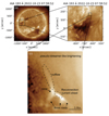 |
Fig. 1. AIA imaging of a pseudo-streamer-like brightening at the coronal hole boundary. |
In the SDO Atmospheric Imaging Assembly (AIA) 193 Å images, the microjet reveals a clear pseudo-streamer-like structure with an extended stalk subjected to intermittent jetting activity situated above a cusp overlying loop-like structures visible at lower altitudes (Fig. 1c). The jet moves along a narrow and bright path away from the solar surface, exhibiting a swaying pattern. As the event evolves, the brightening gradually reveals three bright roots. As discussed later in this paper, these three bright roots and other bright structures correspond to higher-temperature regions in numerical simulations of interchange magnetic reconnection.
We should note that most of the brightenings detected in Hou et al. (2024a) were too small to be resolved as pseudo-streamer-like structures. This should be kept in mind as in the rest of this paper we refer interchangeably to our event as either “the coronal brightening” or “the microjet”. Future studies exploiting higher resolution data such as from Solar Orbiter Extreme-Ultraviolet Imager (EUI; Rochus et al. 2020; Chitta et al. 2023) could investigate further whether all small brightenings exhibit similar pseudo-streamer and jet-like topologies.
Compared to the Helioseismic and Magnetic Imager (HMI) observations of the line-of-sight magnetic field, the photospheric footpoints of three bright roots of the brightening are concentrated in strong magnetic field regions, with a magnetic field strength of approximately 100 G. Based on the linear force-free field extrapolation (Gary 1989) of the magnetic field from the HMI magnetogram, the extrapolated magnetic field lines’ photospheric footpoints are concentrated in three regions of different polarities (Fig. 2a). Among them, the negative-polarity magnetic field lines are relatively concentrated, making it easier to determine the area containing the negative polarity magnetic field and thereby calculate the negative magnetic flux as the jet evolves. The time series of magnetic flux (with a time resolution of 45 seconds) shows that the negative magnetic flux first increases, then decreases, and then increases again, with the rate of change of the surface magnetic flux shown in Fig. 2b. The positive magnetic flux shows no significant trend, possibly due to the relatively dispersed distribution of the positive magnetic field. This makes it challenging to capture the positive magnetic flux during the evolution of the jet accurately.
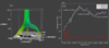 |
Fig. 2. Magnetic field characteristics related to the pseudo-streamer-like brightening. (a) Magnetic field distribution extrapolated from a linear force-free field on an HMI magnetogram. (b) Temporal evolution of the positive and negative photospheric magnetic flux. A movie is available online. |
2.2. Spatio-temporal analysis of the outflowing fluctuations
We analyzed the imaging data by recording brightness variations within slices placed at multiple altitudes along the jetting structure, thereby providing the time-evolving brightness at the SDO AIA time resolution of 12 seconds. In Figs. 3b–h, panels 1 to 7 correspond to from low to high altitudes, where slices 1 to 3 are placed below the cusp and pass through the rapidly evolving base, in what will be shown to be the current sheet of the reconnection event later in the study. Slices 4 to 7 are placed above the cusp through the flow path of the jet extending outward. Each panel in Figs. 3b–h essentially represents a time-space slice (J-map) corresponding to the sampling paths from low to high altitude, clearly showing the structures excited within the reconfiguring magnetic structure, outward-propagating jets, and the fluctuations within the outflow. As the red arrows indicate, the J-map corresponding to slice 2 shows bright points propagating in the opposite direction. The bright points correspond to multiple plasma blobs, likely flux ropes generated by multi-X point reconnection in the current sheet and moving along the current sheet. In the reconnection outflow region corresponding to slices 4 to 7, there are distinct intermittent jets (the jet indicated by the red arrow is the most prominent).
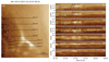 |
Fig. 3. Fine-scale activity and the outflowing fluctuations. (a) AIA 193 Å imaging, with black dashed lines marking the sampling path at multiple altitudes. (b)–(h) Sampling of AIA 193 Å imaging at corresponding altitudes, showing fine-scale activities such as plasma blobs, fluctuations, and jets within the reconnection event. Black arrows indicate the movement directions of plasma blobs and jets. Blue crosses represent wave troughs, and red crosses wave peaks. |
The J-map corresponding to slices 4 to 7 in the reconnection outflow region exhibits distinct transverse oscillations, as indicated by the black dashed lines in Figs. 3b–e. To obtain the amplitude and period of the fluctuations and thereby estimate the energy flux density, we marked the positions of the wave troughs with a blue “x” and the wave peaks with a red “x”. In each panel, we marked two wave troughs and one wave peak. Therefore, we can determine the period and amplitude of the fluctuation before and during the most prominent jet’s appearance. It reveals that the transverse oscillation of the outflow region becomes faster when the jet appears. The appearance of significant magnetic flux ropes and jets coincided with the decreasing phase of negative magnetic flux shown in Fig. 2b. Therefore, this brightening event or magnetic reconnection process is associated with decreased magnetic flux, the appearance of magnetic flux ropes and jets, and transverse oscillation.
The wave energy flux density, Ewave, can be calculated at different altitudes (Morton et al. 2019) via
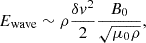 (1)
(1)
where ρ = mne is the mass density, m = 2.12 × 10⁻²⁷ kg is the average mass of ions in a fully ionized plasma (Morton et al. 2019), and ne is the electron number density decreasing with altitude from ∼1010 cm−3 to ∼108 cm−3. The magnetic field strength B0 is obtained from the linear force-free field extrapolation and is approximately 3 G. The amplitude and velocity fluctuation δv can be calculated from the wave peaks and troughs marked in Figs. 3b–e.
In Figs. 3b–e, the energy flux density increases significantly when reconnection occurs (when the most prominent jet is triggered), possibly due to stronger magnetic field line fluctuations generated by the reconfiguring magnetic field. The energy flux density decreases with increasing altitude, which could be attributed to the expansion of the magnetic structure. Considering the super-radial expansion of the magnetic structure (with an expansion factor of 10), the energy flux density at 35 solar radii can be estimated to be approximately 112 W/m W/m2. This result is of the same order of magnitude as the in situ measurements of switchbacks (8000 μW/m2) by PSP at 35 solar radii (Mozer et al. 2020). Moreover, the current calculation of energy flux density is based on the assumption that the polarization direction of the fluctuation is perpendicular to the line of sight. However, the actual polarization direction may not be completely perpendicular to the line of sight and the actual δv could be larger. Therefore, our calculated wave energy flux density should be seen as the lowest bound among all possible real situations.
Using the coronal images of the six AIA extreme ultraviolet (EUV) wavebands, we calculated the differential emission measure (DEM) at the different temperatures (Hannah & Kontar 2012). This spatial distribution of DEM differentiates the various temperature components at the same spatial location. Since the plasma blobs have higher temperature than the surrounding plasma, the DEM could clearly reveal their positions. Figure 4 shows the DEM at two different temperatures before and after the wave-like jet occurs. Before the jet appears (Fig. 4a), the plasma blobs (i.e., magnetic flux ropes) marked by red circle are propagating along the current sheet. The DEM animation (see the supplementary movie of Fig. 4) also observes multiple plasma blobs moving along the reconnection current sheet. When the jet appears (Fig. 4b), the plasma blobs disappear and are replaced by bidirectional flows, significant jet activity, and wave features formed along the reconnection outflow region. The bidirectional flows are also clearly shown in the Doppler velocity distribution provided by the line Fe XII from Hinode Extreme-ultraviolet Imaging Spectrometer (EIS), as illustrated in Fig. 5. In addition, comparing the DEM distributions at the two-time moments, accompanying the bidirectional flows, the amount of high-temperature plasma (T > 106 K) in the cusp region increases (see Figs. 4c and 4d and the corresponding movie).
 |
Fig. 4. DEM distribution before and after the secondary reconnection of flux ropes. A movie is available online. |
 |
Fig. 5. Doppler velocity observations of magnetic reconnection by Hinode/EIS. The black circles mark the locations of the reconnection event. |
3. Magnetic flux emergence and dynamics
To better understand the physical mechanisms behind the dynamics of the brightening presented in the previous sections, we employed a magnetohydrodynamic (MHD) model to simulate the complex dynamics of interchange reconnection that is here likely triggered by magnetic flux emergence and cancellation. We note that the actual trigger mechanism of solar jets remains debated (Pariat et al. 2010; Innes & Teriaca 2013; Panesar et al. 2016; Kumar et al. 2019a; Pariat et al. 2023). We first describe the methodology and model configuration adopted in this study (Sect. 3.1), including the initial conditions and boundary specifications relevant to the inserted bipole (Sect. 3.2).
3.1. Simulation setup and fundamental equations
The simulation is conducted within a 2.5D Cartesian domain x = [ − 25, 26] Mm and y = [0, 60] Mm. The time evolution of macroscopic physical quantities, including the magnetic field (B), plasma velocity (v), density (ρ), pressure (p), and the current density (J), is governed by the following set of resistive MHD equations:
 (2)
(2)
 (3)
(3)
![Mathematical equation: $$ \begin{aligned}&\frac{\partial }{\partial t}E + \nabla \cdot \left[(E + p) \boldsymbol{v} - \boldsymbol{B} (\boldsymbol{v} \cdot \boldsymbol{B}) + (\eta \cdot \boldsymbol{J}) \times \boldsymbol{B}\right] = Q_{\rm h} - Q_{\rm c} - Q_{\rm r}, \end{aligned} $$](/articles/aa/full_html/2025/05/aa53237-24/aa53237-24-eq5.gif) (4)
(4)
 (5)
(5)
![Mathematical equation: $$ \begin{aligned}&\boldsymbol{J} = \frac{1}{\mu _0} [\boldsymbol{\nabla } \times \boldsymbol{B}], \end{aligned} $$](/articles/aa/full_html/2025/05/aa53237-24/aa53237-24-eq7.gif) (6)
(6)
 (7)
(7)
Here, μ0 represents the magnetic permeability in a vacuum, and η denotes the resistivity. The specific heat ratio is Γ = 5/3. The temperature T is derived using the relation  , where kB is the Boltzmann constant, and 0.5 mp is the average mass of fully ionized hydrogen. Gravitational acceleration, g, is constant, 274 m/s2, and acts downward along the y-axis.
The energy equation incorporates various source terms including a constant heating source Qh = 10−5 erg cm−3 s−1 = 10−6 J m−3 s−1, conductive energy transport Qc, and radiative losses Qrad. The thermal conductivity is aligned with the magnetic field:
 (8)
(8)
where κ∥ = 5.6 × 10⁻⁷ T5/2 erg s−1 K−1 cm−1, and  is the unit vector along the magnetic field.
We employed an optically thin radiative cooling defined as
 (9)
(9)
where n is the electron density, T is the electron temperature, and Λ is calculated using the CHIANTI database (version 10.0.1) radiative loss function, fitted for solar coronal abundances (Dere et al. 1997; Del Zanna et al. 2021; Schmelz et al. 2012).
The governing equations are solved using the PLUTO code (Mignone et al. 2007), with a computational cartesian grid consisting of 1800 × 2048 uniformly distributed elements along the x- y-axes and one element along z-axes. We utilized the Harten-Lax-van Leer discontinuities (HLLD) Riemann solver (Miyoshi & Kusano 2005) to manage discontinuities and sharp gradients effectively. Moreover, a constrained transport method (Balsara & Spicer 1999) is implemented to maintain the divergence-free condition of the magnetic field (∇⋅B = 0). Temporal discretization is handled using the Runge-Kutta second-order (RK2) method, and parabolic reconstruction is applied to reconstruct cell surface quantities.
The lower boundary acts as a dynamic driver, simulating the emergence and cancellation of a magnetic bipole. Lateral boundaries are defined as outflow conditions ![Mathematical equation: $ (\frac{\partial [\boldsymbol{B}, \rho, p, \boldsymbol{v}]}{\partial n} = 0) $](/articles/aa/full_html/2025/05/aa53237-24/aa53237-24-eq13.gif) , while the upper boundary permits outflow for all variables except pressure, which undergoes linear extrapolation.
, while the upper boundary permits outflow for all variables except pressure, which undergoes linear extrapolation.
3.2. Initial conditions and lower boundary specifications
The initial atmospheric domain follows a stratified profile along the y-axes and uniform along the x-axis, with density and temperature distributions aligned with the empirical solar model of Vernazza et al. (1981). The density at the upper photosphere is approximately 4.08 × 10⁻⁸ kg m−3, with a temperature of around 3000 K. Moving into the chromosphere, the density exponentially decreases with a scale height of 1 Mm, while the temperature increases sharply to about 1.2 MK at heights of 2−2.5 Mm. The coronal region is characterized by a nearly constant temperature and a slight reduction in density, reaching 5 × 10⁻¹³ kg m−3 (N ∼ 1014 m−3).
The initial density distribution is defined as
 (10)
(10)
where ych is a parameter that adjusts the vertical position of the profile. The pressure profile is obtained by integrating the hydrostatic equilibrium equation  , and the temperature is derived from the ideal gas law. This profile is adapted from the works of Gordovskyy et al. (2014) and Pinto et al. (2016).
In Fig. 6 the right panel shows the plasma density ρ (in kg/m−3) as a function of height, while the left panel displays the plasma temperature T (in MK) across the same range. The solid lines indicate the initial state of the plasma, whereas the dashed lines show the state after the thermal relaxation phase has concluded. This comparison shows how both plasma density and temperature evolve during this phase. For the present simulation, we used the following normalization parameters: L0 = 106 m, U0 = 4.3670 × 10⁷ m s−1, and ρ0 = 1.67 × 10⁻¹² kg m−3, which yield a characteristic magnetic field B0 = 200 G and a characteristic time of t0 = 2.28 s.
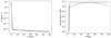 |
Fig. 6. Plasma density, ρ (in kg/m−3; left) and plasma temperature, T (in MK; right), both as functions of height during the preparatory thermal relaxation phase at two different positions above the surface. Solid lines represent the initial state, and dashed lines the final state after the thermal relaxation phase. |
3.3. Flux emergence and cancellation
In various numerical simulations and magnetic reconnection models, the triggering mechanisms for magnetic reconnection are diverse. For example, the emergence of magnetic flux (Moreno-Insertis et al. 2018) can induce reconnection, where the compression between closed magnetic loops and the preexisting field is a common triggering mechanism (Shibata et al. 1992; Moreno-Insertis & Galsgaard 2013; Gannouni et al. 2023). Additionally, the magnetic flux cancellation is another important process, often accompanied by the convergence of opposite-polarity magnetic field lines driven by photospheric convection (Sterling et al. 2018; Innes & Teriaca 2013; Panesar et al. 2016). Furthermore, the shearing motion of magnetic loop footpoints caused by the convection (Yang et al. 2015; Wyper et al. 2017; He et al. 2021) can also lead to the uplift of magnetic loops, compressing the background field and ultimately triggering magnetic reconnection. In addition to footpoint motions, the stressing at the interface between closed loops and preexisting open fields may also serve as a trigger for magnetic reconnection, as analyzed in a 3D MHD simulation using HMI observations as the initial magnetic configuration (Galsgaard et al. 2015). Some more intricate reconnection models for jets and brightenings takes into account the twisted magnetic structures generated by footpoint motions, as analyzed through 3D simulations (Galsgaard et al. 2019) and observations (Moore et al. 2010).
For the reconnection event in our work, we find that the blowout of the jet was preceded by an increasing magnetic flux rather than a decrease, suggesting that the trigger of magnetic reconnection was more likely due to magnetic flux emergence rather than cancellation. SDO/HMI magnetograms show that during the flux emergence, the concentration regions with opposite-polarity magnetic fields moved apart (see the supplementary movie of Fig. 2), consistent with the uplift of closed magnetic loop and the separation of its footpoints. Moreover, no significant shearing motion was observed during this separation process. Therefore, we consider magnetic loop emergence (Moreno-Insertis & Galsgaard 2013) to be the most probable mechanism for triggering magnetic reconnection in our event and thus performed high-resolution 2.5D numerical simulations based on this scenario.
The initial configuration of the magnetic field assumes a background magnetic field inclined at an angle of 26° relative to the vertical axis, in accordance with the observation shown in Fig. 1c, with an initial magnetic field strength of 3 G. Following the relaxation phase, a bipole with an increasing magnetic field strength is introduced into the lower boundary condition of the domain. This bipole gradually emerges, reaching a peak amplitude of approximately 1019 Mx. Once this peak is achieved, the simulation is allowed to relax, with the bipole held at a constant amplitude for an additional 25 minutes of simulation time (see Fig. 7).
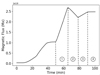 |
Fig. 7. Evolution during flux emergence and flux cancellation. After the thermal relaxation phase, the flux emergence begins with a rate of 6.9 × 10¹⁹ Mx/h (labeled 1 in the plot). This is followed by a decrease in magnetic flux with a slope of −2.3 × 10¹⁹ Mx/h (labeled 2). The magnetic flux then increases again at a rate of 1.2 × 10¹⁹ Mx/h (labeled 3), before a final relaxation phase is observed (labeled 4). Phases (1), (2), and (3) correspond to the three phases of negative magnetic flux shown in Fig. 2b. |
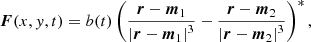
Subsequently, the simulation follows an emergence rate provided directly from the observational flux emergence and cancellation rates labeled in Fig. 2. To generate the bipole, we employed the potential field bipole expression, F, imposed as the driving condition at the lower boundary:
 (11)
(11)
In this equation, b(t) represents the time-varying amplitude of the magnetic field, which drives the emergence and cancellation of the bipole’s flux. The vector r corresponds to the position, while m1 and m2 define the positions of the monopoles, specified by m1 = [a, −h] and m2 = [ − a, −h], respectively. The parameter h denotes the depth of the monopoles, influencing the convergence of the magnetic field lines toward the footpoints. In our simulations we used the values a = 1.5L0 and h = 1.1L0 (* refer to normalization units).
3.4. Numerical results
3.4.1. Synthetic imagery of the microjet
To enable a detailed comparison of our simulation results with the AIA observations, we produced synthetic imagery in 193 Å directly from our the temperatures and densities calculated by our numerical model. The spectral response function is provided by the AIA instrument team and the contribution function is calculated using the CHIANTI atomic physics database version 7.1.3 and ChiantiPy interface (Dere et al. 1997; Dere 2013) and assuming ionization equilibrium and coronal composition. The reader is referred to Gannouni et al. (2023) for additional information on this approach. Figure 8 provides a comprehensive overview of the magnetic bipole’s evolution and associated wave dynamics during the flux emergence and cancellation process. As illustrated in the Fig. 8a, it depicts the magnetic bipole at 61 minutes, approximately 10 minutes after the onset of the emergence phase.
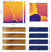 |
Fig. 8. Upper left: Magnetic bipole at 61 minutes, approximately 10 minutes into the emergence phase. Four distinct horizontal slices are marked in yellow to indicate the regions where synthetic emission and Alfvén wave energy flux were calculated over time. Upper right: Zoom-in of the current sheet region, where the plasma blobs are clearly seen. Lower left: Time series of synthetic emission in the 193 Å wavelength for the four horizontal lines. Lower right: Alfvén wave energy flux density for the same four horizontal lines. |
In the simulation, as the reconnecting current sheet gradually thins, magnetic reconnection process occurs. The current sheet contains numerous plasmoids at higher temperatures enclosed by magnetic islands (Fig. 8b). Multi-point, multi-scale plasmoids indicate that the tearing-mode instability drives the onset conditions of the magnetic reconnection process (Furth et al. 1963). Similar results, featuring plasmoids and subsequent eruptions, are also shown in a 3D reconnection simulation where magnetic loop emergence serves as the trigger mechanism (Archontis et al. 2006; Moreno-Insertis & Galsgaard 2013), 2.5D reconnection simulation driven by moving magnetic footpoints (Yang et al. 2013), 2D resistive MHD reconnection simulations driven by flux emergence (Ni et al. 2017; Nóbrega-Siverio & Moreno-Insertis 2022) and coronal EUV observations (Kumar et al. 2019b). We carefully chose η such that the tearing instability is triggered, that is, to ensure that the Lundquist number is bigger than 104 (Loureiro et al. 2007; Bhattacharjee et al. 2009). The theoretical work of Pucci & Velli (2013) have shown that once a sufficiently high Lundquist number is achieved in a thinning current sheet, the tearing instability developed with an “ideal” growth rate, independent of resistivity. In our simulation, the magnetic diffusivity is set to η = 5 × 1011 cm2/s = 5 × 10⁷ m2/s, and the Lundquist number Lq near the current sheet is approximately 5 × 10⁴. This approach has previously been employed for similar purposes in Réville et al. (2020) and Gannouni et al. (2023).
In our simulation, the magnetic islands generated by the reconnection process move along the reconnection current sheet, either toward the newly opened magnetic field lines or toward low altitudes, and evolve as closed magnetic fields confined in the low atmosphere. The outward and inward motions of these magnetic islands resemble closely the plasma blobs observed in the SDO AIA images and described in the previous section.
Wave-like oscillations are observed in the jet are driven by the islands reaching the newly opened field lines extending outward above the cusp of the formed pseudo-streamer structure as already discussed in Gannouni et al. (2023). Just as we did for the SDO AIA image analysis in Sect. 2, we extracted a band of pixels along the slices shown in Figs. 8c1–c4 to isolate the time-evolving transverse oscillations at different altitudes. The time series of synthetic emission at a wavelength of 193 Å along the four marked slices are shown in Figs. 8c1–c4. The corresponding wave energy flux (Figs. 8d1–d4 is consistent with our observational value derived from Figs. 3b–e.
Regarding Fig. 8, it is important to note that in the zoomed-in images of panels (c1–c4) and (d1–d4) we can see oscillating patterns that are comparable to those of the observations. This reinforces the idea that this small-scale activity of observed jet propagates as a wave-like packet. Additionally, it is evident that as the magnitude of emergence increases, it significantly influences the wave flux density with a maximum value about 400 W/m2. Notably, the amplitude of the wave does not decay easily during propagation. This is expected if the wave is an incompressible Alfvén wave characterized by low dissipation.
3.4.2. Recurrence and Alfvénicity of wave-like jets
Simulations exhibit recurrent wave-like jets originating from the cusp region, where plasma blobs continually collision with the open field lines, initiating a sequence of plasma and magnetic field fluctuations. Figure 9 shows the maximum vertical velocity achieved over the entire simulation period, with the comparison to observed data beginning at the onset of magnetic flux emergence, approximately 50 minutes into the simulation. The results demonstrate that the flux emergence and subsequent cancellation significantly influence the velocity of the triggered jets, which range from 10 to 80 km/s.
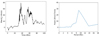 |
Fig. 9. Left: Maximum vertical velocities simulated at a height of 17.6 Mm above the bipole cusp. Right: Power spectral density analysis revealing the dominant periods of the simulated velocity oscillations shown in the left-hand panel. |
We conducted a Fourier analysis to identify the dominant or recurring periods within the wave-like jets. Prior to applying the fast Fourier transform, we removed the mean value from the time series data in Fig. 9 and commenced after the initial relaxation phase, approximately 50 minutes into the simulation. The power spectral density shown in Fig. 9 has a dominant oscillation period of 9 minutes. This is in line with periodicities also modeled in Gannouni et al. (2023) and aligns with PSP radial velocity spikes observations reported in Fargette et al. (2021), Kumar et al. (2023).
To investigate the Alfvénic properties of the generated wave-like jets, we adopted the following approach. First, the position of the jet was localized by identifying the point of maximum vertical velocity. Next, fluctuations in both the magnetic field (including its components and magnitude) and plasma velocity (radial and tangential components) were computed. To remove background trends, a linear fit was subtracted from the raw data. The resulting perturbed signals were then normalized, ensuring a mean of zero and a standard deviation of one.
Figure 10 presents time series data at two altitudes (17.6 Mm and 29.3 Mm), illustrating the magnetic field components and total magnitude, the velocity components, the Alfvén and plasma velocity fluctuations in three spatial directions, and the relative density normalized to the initial plasma density. The relation δuA ≈ −δv strongly supports the Alfvénic nature of the jet (Fig. 10), which is propagating outward. All velocity components exhibit invariance with increasing altitude, indicating that the jet becomes less compressible at higher altitudes. These characteristics align well with the behavior of incompressible Alfvén wave, given the constraints  and |B|≈const.
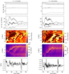 |
Fig. 10. Comparison of magnetic field, velocity, and Alfvénic wave fluctuations at 17.6 Mm and 29.30 Mm altitudes, demonstrating the wave-like jet’s characteristics. |
3.4.3. Comparison with imaging observations
The observations and simulations exhibit similar characteristics during these cycles of magnetic reconnection are producing plasma blobs ejected and triggering sequences of recurrent wave-like jets. The observations and simulations show a high degree of consistency, particularly in the key aspects of our main focus.
As introduced in Sect. 3.1, we established the magnetic flux emergence and cancellation rates in our simulations to match observational values (Fig. 2b). In the subsequent evolution of simulated reconnection, the sizes of micro-jets observed and simulated are consistent. Given that AIA images only capture the projection of micro-jets on the sky plane, we incorporated Solar Orbiter/EUI Full Sun Imager images of the same micro-jets to reconstruct their height and direction in 3D space. This allowed us to calculate the height of the cusp regions, approximately 6 Mm above the photosphere, which aligns well with the simulated value of around 7 Mm (Fig. 8a). Additionally, by identifying the outflow region’s direction, we obtained the actual propagation speed of the micro-jets, approximately 225 km/s, based on the projecting speed of about 210 km/s calculated from the J-map (Fig. 3). It is important to note that the propagation speed represents the sum of the jet’s speed in the solar wind reference frame and the speed of the background solar wind. In the simulations, the jet speed in the solar wind reference frame ranges from 10 to 80 km/s. Accounting for the simulation background solar wind speed, the total speed of simulation jets approximates 200 km/s, which is consistent with real observations. Therefore, the initial simulation setup and the subsequent evolution of interchange reconnection align with actual observations and could effectively highlight the fine-scale characteristics of reconnections.
As illustrated in the Figs. 3 and 8a, b and described in the previous sections, three types of fine-scale activities were observed in both the imaging of this coronal brightening event and the corresponding simulations: magnetic flux ropes, waves, and jet activities. Among them, the signals in the high-resolution numerical simulations are more distinct than those in the observations. Also shown in Figs. 8a, b, multiple plasma blobs appear in high spatial resolution simulations within the initial reconnection current sheet. As these plasma blobs move outward and come into contact with the open field lines, they lead to waves in the outflow region, and the generation of intermittent jets.
As shown in the Figs. 3 and 8, the wave energy flux density calculated from the SDO AIA images is approximately 112 W/m2 at the cusp region. We also note that, considering the projection of wave polarization in the plane perpendicular to the line of sight, this wave energy flux should be regarded as a lower bound of the true value. In numerical simulations, we can fully capture the velocity and magnetic field fluctuations at each location. Thus, the simulations provide a wave energy flux ranging from 100 W/m2 to 400 W/m2, which is consistent with the results obtained from observations.
After the interaction between the flux rope and the open field lines in the cusp region, both observations and simulations show consistent temperature variation characteristics. DEM analysis of the observations (Fig. 4 and corresponding animation) indicates that, after the flux rope moves into the cusp, the amount of plasma with temperatures below 106 K decreases, while plasma with temperatures above 1.3 × 10⁶ K increases. Additionally, the heated plasma exhibits a long, strip-like distribution along magnetic field lines. The temperature distribution from numerical simulations (Figs. 8a and 8b) shows similar characteristic that the interaction between the flux rope and the open field lines leads to the formation of a high-temperature area along the open field lines in the cusp region, with temperatures around 1.2 × 10⁶ K. These results indicate a strong consistency between the observations and the numerical simulations.
4. Discussion
The aim of the paper was to analyze the structure and evolution of a small solar brightening observed in the estimated source region of velocity spikes and switchbacks measured by Solar Orbiter in Hou et al. (2024a). By conducting a comprehensive data analysis from multiple remote-sensing instruments, we could extract important information on the dynamic evolution of fine-scale magnetic flux ropes, their interactions with surrounding magnetic field lines, and the wave amplitudes excited by magnetic reconnection. The analysis of AIA observations reveal that small-scale current sheets can produce multiple propagating plasma blobs. These magnetic islands or magnetic flux ropes are seen propagating outward, and AIA observations show that they rapidly fade in observations and that their properties (temperature and density) evolve rapidly with height, suggesting a secondary processing, perhaps secondary magnetic reconnection. This magnetic reconnection leads to outward propagating oscillations escaping along with jet. The energy flux densities are similar in the observations and simulations and comparable to those inferred from in situ measurements of magnetic switchbacks.
We used high-resolution 2.5D MHD simulations to shed additional light on the processes involved in the different regions and phases of the jet formation and release mechanisms observed in remote-sensing observations. In our numerical simulations, the formation of wave-like jets is closely associated with the continuous generation and ejection of plasma blobs from the current sheet. The simulations demonstrate that the emergence and subsequent cancellation of magnetic flux significantly impact the jet velocities, ranging from 10 to 80 km/s. Fourier analysis identified a dominant recurrence period of 9 minutes for jets, consistent with observational data. Alfvén waves revealed the characteristics of spherical polarization; as wave amplitudes increase with a decaying background magnetic field, the local magnetic field can reverse, resembling switchbacks. Additionally, secondary magnetic reconnection is validated in the simulations, showing how interactions between magnetic flux ropes and open field lines trigger jet and wave activity, in which energy flux density is consistent with the observational values. These results further support the idea that reconnection-driven waves plays a crucial role in the formation of interplanetary magnetic switchbacks and velocity spikes.
We find the simulations that large-amplitude Alfvén waves are formed by a secondary reconnection process that erodes the magnetic islands in the open magnetic field. The outflowing waves and the jets may precondition the medium for the formation of interplanetary magnetic switchbacks and velocity spikes. The amplitude growth and steepening process of Alfvén waves expected in the upper corona and the formation of density fluctuations in the solar wind deserve further in-depth investigation, whether through coordinated multi-satellite measurements or high-resolution numerical simulations.
Squire et al. (2020) demonstrated how Alfvén waves reverse magnetic field lines during their propagation through numerical simulations of an expanding solar wind. Hou et al. (2023) combined statistical characteristics of magnetic kinks and switchbacks and proposed that the coupling of Alfvén waves and magnetosonic waves generated by reconnection can form stable rotational discontinuities, leading to magnetic field direction changes similar to switchbacks. Our results further confirm that the energy flux density of reconnection-triggered waves is sufficient to support the formation of interplanetary switchbacks. In addition to wave activity, plasma motions associated with shear and interactions with the solar wind may also contribute to the formation of switchbacks. During the development of the plumes, small jets (jetlets) could increase bulk flow kinetic energy to coronal plumes and lead to intermittent outflows and velocity spikes (Raouafi et al. 2023; Kumar et al. 2023). Furthermore, switchbacks can appear in the turbulent solar wind, as simulated by Shoda et al. (2021), and turbulence energy could also be converted from jets’ kinetic energy (Ruan et al. 2023). To assess and rank the contributions of plasma jets and wave packets, we need to conduct the simulations to show the evolution of wave-like jets within the interplanetary solar wind. This additional research will be carried out in future work.
5. Summary
We conclude that the small-scale dynamics of the microjet are driven by magnetic reconnection. Based on observations and our 2.5D MHD simulations, we find that the released magnetic islands undergo secondary reconnection, which produces bursts of small jets and large-amplitude magnetic fluctuations that propagate into the solar wind. We propose that these waves evolve into bursts of switchbacks and velocity spikes in the upper corona, where the velocity shear induced by jets may amplify and fold large-amplitude Alfvénic fluctuations. As these waves grow in the decaying background magnetic field, the increasing ratio of fluctuation to the background field could lead to local reversals of magnetic field polarity (Squire et al. 2020; Mallet et al. 2021; Matteini et al. 2024) that resemble the switchbacks observed in the solar wind. Our findings suggest that reconnection-driven waves play a critical role in shaping the dynamics of interplanetary switchbacks and velocity spikes, providing important insights into the mechanisms underlying solar wind variability.
Solar Orbiter/EUI (Rochus et al. 2020) can provide higher-resolution images of the internal activities of jet events (Chitta et al. 2021). Our analysis can be applied to these images for individual events and statistical studies of jet triggers and associated activities. Furthermore, by combining high-resolution EUV images with spectroscopic measurements from Hinode/EIS (Young et al. 2007; Brooks & Warren 2010) and Solar Orbiter’s SPICE (Anderson et al. 2020) instrument, we aim to determine the elemental abundance variations and the Doppler velocity at different jet event locations. This could include differences in elemental abundances and motion before and after magnetic reconnection, open and closed field lines, magnetic flux ropes, and the surrounding plasma. By correlating these results with in situ solar wind elemental abundance measurements, we can more accurately pinpoint the origin and timing of interplanetary switchbacks in the solar atmosphere.
Data availability
Movies associated to Figs. 2 and 4 are available at https://www.aanda.org
Acknowledgments
We acknowledge the solar wind measurements from Proton Alpha Sensor (PAS) aboard Solar Orbiter, remote sensing imagery SDO, and magnetograms from GONG. The work at Peking University is supported by National Key R&D Program of China (2021YFA0718600 and 2022YFF0503800), by NSFC (42241118, 42174194, 42150105, and 42204166), and by CNSA (D020301 and D050106). The work at IRAP carried out by CH, BG, APR and VR was funded by the ERC SLOW_SOURCE project (SLOW_SOURCE–DLV-819189) and CNES through the APR program. This work was granted access to the HPC resources of IDRIS under the allocation 2024-A0170410293 made by GENCI. CH is also supported by the China Scholarship Council (202206010136). This research was supported by the International Space Science Institute (ISSI) in Bern through ISSI International Team project #463 (Exploring The Solar Wind In Regions Closer Than Ever Observed Before) led by L. Harra.
References
- Anderson, M., Appourchaux, T., Auchère, F., et al. 2020, A&A, 642, A14 [NASA ADS] [CrossRef] [EDP Sciences] [Google Scholar]
- Archontis, V., Galsgaard, K., Moreno-Insertis, F., & Hood, A. W. 2006, ApJ, 645, L161 [NASA ADS] [CrossRef] [Google Scholar]
- Bale, S., Badman, S., Bonnell, J., et al. 2019, Nature, 576, 237 [Google Scholar]
- Bale, S. D., Horbury, T., Velli, M., et al. 2021, ApJ, 923, 174 [NASA ADS] [CrossRef] [Google Scholar]
- Balsara, D. S., & Spicer, D. S. 1999, J. Comput. Phys., 149, 270 [NASA ADS] [CrossRef] [Google Scholar]
- Bhattacharjee, A., Huang, Y.-M., Yang, H., & Rogers, B. 2009, Phys. Plasmas, 16, 112102 [Google Scholar]
- Brooks, D. H., & Warren, H. P. 2010, ApJ, 727, L13 [Google Scholar]
- Chandrashekhar, K., Bemporad, A., Banerjee, D., Gupta, G., & Teriaca, L. 2014, A&A, 561, A104 [NASA ADS] [CrossRef] [EDP Sciences] [Google Scholar]
- Chitta, L., Solanki, S. K., Peter, H., et al. 2021, A&A, 656, L13 [NASA ADS] [CrossRef] [EDP Sciences] [Google Scholar]
- Chitta, L., Zhukov, A., Berghmans, D., et al. 2023, Science, 381, 867 [NASA ADS] [CrossRef] [Google Scholar]
- Cirtain, J., Golub, L., Lundquist, L., et al. 2007, Science, 318, 1580 [Google Scholar]
- Del Zanna, G., Dere, K. P., Young, P. R., & Landi, E. 2021, ApJ, 909, 38 [NASA ADS] [CrossRef] [Google Scholar]
- Dere, K. 2013, Astrophysics Source Code Library [record ascl:1308.017] [Google Scholar]
- Dere, K. P., Landi, E., Mason, H. E., Monsignori Fossi, B. C., & Young, P. R. 1997, A&AS, 125, 149 [NASA ADS] [CrossRef] [EDP Sciences] [Google Scholar]
- Drake, J., Agapitov, O., Swisdak, M., et al. 2021, A&A, 650, A2 [NASA ADS] [CrossRef] [EDP Sciences] [Google Scholar]
- Fargette, N., Lavraud, B., Rouillard, A. P., et al. 2021, ApJ, 919, 96 [NASA ADS] [CrossRef] [Google Scholar]
- Furth, H. P., Killeen, J., & Rosenbluth, M. N. 1963, Phys. Fluids, 6, 459 [Google Scholar]
- Galsgaard, K., Madjarska, M., Vanninathan, K., Huang, Z., & Presmann, M. 2015, A&A, 584, A39 [NASA ADS] [CrossRef] [EDP Sciences] [Google Scholar]
- Galsgaard, K., Madjarska, M. S., Mackay, D. H., & Mou, C. 2019, A&A, 623, A78 [NASA ADS] [CrossRef] [EDP Sciences] [Google Scholar]
- Gannouni, B., Réville, V., & Rouillard, A. P. 2023, ApJ, 958, 110 [NASA ADS] [CrossRef] [Google Scholar]
- Gary, G. A. 1989, ApJS, 69, 323 [Google Scholar]
- Gordovskyy, M., Browning, P. K., Kontar, E. P., & Bian, N. H. 2014, A&A, 561, A72 [NASA ADS] [CrossRef] [EDP Sciences] [Google Scholar]
- Griton, L., Pinto, R. F., Poirier, N., et al. 2020, ApJ, 893, 64 [Google Scholar]
- Hannah, I. G., & Kontar, E. P. 2012, A&A, 539, A146 [NASA ADS] [CrossRef] [EDP Sciences] [Google Scholar]
- He, J., Zhu, X., Yang, L., et al. 2021, ApJ, 913, L14 [NASA ADS] [CrossRef] [Google Scholar]
- Hou, C., Zhu, X., Zhuo, R., et al. 2023, ApJ, 950, 157 [NASA ADS] [CrossRef] [Google Scholar]
- Hou, C., Rouillard, A. P., He, J., et al. 2024a, ApJ, 968, L28 [NASA ADS] [CrossRef] [Google Scholar]
- Hou, C., He, J., Duan, D., et al. 2024b, Nat. Astron., 8, 1246 [Google Scholar]
- Innes, D. E., & Teriaca, L. 2013, Sol. Phys., 282, 453 [CrossRef] [Google Scholar]
- Kasper, J. C., Bale, S. D., Belcher, J. W., et al. 2019, Nature, 576, 228 [Google Scholar]
- Kumar, P., Karpen, J. T., Antiochos, S. K., et al. 2019a, ApJ, 873, 93 [NASA ADS] [CrossRef] [Google Scholar]
- Kumar, P., Karpen, J. T., Antiochos, S. K., Wyper, P. F., & DeVore, C. R. 2019b, ApJ, 885, L15 [Google Scholar]
- Kumar, P., Karpen, J. T., Uritsky, V. M., et al. 2023, ApJ, 951, L15 [CrossRef] [Google Scholar]
- Liu, W., Berger, T. E., Tarbell, T. D., et al. 2009, ApJ, 707, L37 [Google Scholar]
- Loureiro, N. F., Schekochihin, A. A., & Cowley, S. C. 2007, Phys. Plasmas, 14, 100703 [NASA ADS] [CrossRef] [Google Scholar]
- Madjarska, M. S. 2019, Liv. Rev. Sol. Phys., 16, 2 [Google Scholar]
- Mallet, A., Squire, J., Chandran, B. D., Bowen, T., & Bale, S. D. 2021, ApJ, 918, 62 [NASA ADS] [CrossRef] [Google Scholar]
- Matteini, L., Tenerani, A., Landi, S., et al. 2024, Phys. Plasmas, 31, 032901 [NASA ADS] [CrossRef] [Google Scholar]
- Mignone, A., Bodo, G., Massaglia, S., et al. 2007, ApJS, 170, 228 [Google Scholar]
- Miyoshi, T., & Kusano, K. 2005, J. Comput. Phys., 208, 315 [NASA ADS] [CrossRef] [Google Scholar]
- Moore, R. L., Cirtain, J. W., Sterling, A. C., & Falconer, D. A. 2010, ApJ, 720, 757 [Google Scholar]
- Moreno-Insertis, F., & Galsgaard, K. 2013, ApJ, 771, 20 [Google Scholar]
- Moreno-Insertis, F., Martinez-Sykora, J., Hansteen, V., & Muñoz, D. 2018, ApJ, 859, L26 [Google Scholar]
- Morton, R., Weberg, M., & McLaughlin, J. 2019, Nat. Astron., 3, 223 [NASA ADS] [CrossRef] [Google Scholar]
- Mozer, F., Agapitov, O., Bale, S., et al. 2020, ApJS, 246, 68 [NASA ADS] [CrossRef] [Google Scholar]
- Nakariakov, V., Ofman, L., & Arber, T. 2000, A&A, 353, 741 [Google Scholar]
- Ni, L., Zhang, Q.-M., Murphy, N. A., & Lin, J. 2017, ApJ, 841, 27 [Google Scholar]
- Nóbrega-Siverio, D., & Moreno-Insertis, F. 2022, ApJ, 935, L21 [CrossRef] [Google Scholar]
- Panesar, N. K., Sterling, A. C., Moore, R. L., & Chakrapani, P. 2016, ApJ, 832, L7 [Google Scholar]
- Pariat, E., Antiochos, S. K., & DeVore, C. 2010, ApJ, 714, 1762 [NASA ADS] [CrossRef] [Google Scholar]
- Pariat, E., Wyper, P., & Linan, L. 2023, A&A, 669, A33 [NASA ADS] [CrossRef] [EDP Sciences] [Google Scholar]
- Pesnell, W. D., Thompson, B. J., & Chamberlin, P. 2012, Sol. Phys., 275, 3 [NASA ADS] [CrossRef] [Google Scholar]
- Pinto, R. F., Gordovskyy, M., Browning, P. K., & Vilmer, N. 2016, A&A, 585, A159 [NASA ADS] [CrossRef] [EDP Sciences] [Google Scholar]
- Pucci, F., & Velli, M. 2013, ApJS, 780, L19 [Google Scholar]
- Raouafi, N. E., Stenborg, G., Seaton, D. B., et al. 2023, ApJ, 945, 28 [NASA ADS] [CrossRef] [Google Scholar]
- Réville, V., Velli, M., Rouillard, A. P., et al. 2020, ApJ, 895, L20 [Google Scholar]
- Rochus, P., Auchere, F., Berghmans, D., et al. 2020, A&A, 642, A8 [NASA ADS] [CrossRef] [EDP Sciences] [Google Scholar]
- Rouillard, A. P., Kouloumvakos, A., Vourlidas, A., et al. 2020, ApJS, 246, 37 [Google Scholar]
- Ruan, W., Yan, L., & Keppens, R. 2023, ApJ, 947, 67 [NASA ADS] [CrossRef] [Google Scholar]
- Schmelz, J. T., Reames, D. V., von Steiger, R., & Basu, S. 2012, ApJ, 755, 33 [NASA ADS] [CrossRef] [Google Scholar]
- Shen, Y. 2021, PRSA, 477, 20200217 [Google Scholar]
- Shibata, K., Ishido, Y., Acton, L. W., et al. 1992, PASJ, 44, L173 [Google Scholar]
- Shoda, M., Chandran, B. D., & Cranmer, S. R. 2021, ApJ, 915, 52 [CrossRef] [Google Scholar]
- Squire, J., Chandran, B. D., & Meyrand, R. 2020, ApJ, 891, L2 [NASA ADS] [CrossRef] [Google Scholar]
- Sterling, A. C., Moore, R. L., Falconer, D. A., & Adams, M. 2015, Nature, 523, 437 [NASA ADS] [CrossRef] [Google Scholar]
- Sterling, A. C., Moore, R. L., & Panesar, N. K. 2018, ApJ, 864, 68 [NASA ADS] [CrossRef] [Google Scholar]
- Vernazza, J. E., Avrett, E. H., & Loeser, R. 1981, ApJS, 45, 635 [Google Scholar]
- Wyper, P. F., Antiochos, S. K., & DeVore, C. R. 2017, Nature, 544, 452 [Google Scholar]
- Yang, L., He, J., Peter, H., et al. 2013, ApJ, 777, 16 [NASA ADS] [CrossRef] [Google Scholar]
- Yang, L., Zhang, L., He, J., et al. 2015, ApJ, 809, 155 [Google Scholar]
- Young, P. R., Zanna, D. G., Mason, H. E., et al. 2007, PASJ, 59, S857 [NASA ADS] [CrossRef] [Google Scholar]
All Tables
All Figures
|
Fig. 1. AIA imaging of a pseudo-streamer-like brightening at the coronal hole boundary. |
| In the text | |
|
Fig. 2. Magnetic field characteristics related to the pseudo-streamer-like brightening. (a) Magnetic field distribution extrapolated from a linear force-free field on an HMI magnetogram. (b) Temporal evolution of the positive and negative photospheric magnetic flux. A movie is available online. |
| In the text | |
|
Fig. 3. Fine-scale activity and the outflowing fluctuations. (a) AIA 193 Å imaging, with black dashed lines marking the sampling path at multiple altitudes. (b)–(h) Sampling of AIA 193 Å imaging at corresponding altitudes, showing fine-scale activities such as plasma blobs, fluctuations, and jets within the reconnection event. Black arrows indicate the movement directions of plasma blobs and jets. Blue crosses represent wave troughs, and red crosses wave peaks. |
| In the text | |
|
Fig. 4. DEM distribution before and after the secondary reconnection of flux ropes. A movie is available online. |
| In the text | |
|
Fig. 5. Doppler velocity observations of magnetic reconnection by Hinode/EIS. The black circles mark the locations of the reconnection event. |
| In the text | |
|
Fig. 6. Plasma density, ρ (in kg/m−3; left) and plasma temperature, T (in MK; right), both as functions of height during the preparatory thermal relaxation phase at two different positions above the surface. Solid lines represent the initial state, and dashed lines the final state after the thermal relaxation phase. |
| In the text | |
|
Fig. 7. Evolution during flux emergence and flux cancellation. After the thermal relaxation phase, the flux emergence begins with a rate of 6.9 × 10¹⁹ Mx/h (labeled 1 in the plot). This is followed by a decrease in magnetic flux with a slope of −2.3 × 10¹⁹ Mx/h (labeled 2). The magnetic flux then increases again at a rate of 1.2 × 10¹⁹ Mx/h (labeled 3), before a final relaxation phase is observed (labeled 4). Phases (1), (2), and (3) correspond to the three phases of negative magnetic flux shown in Fig. 2b. |
| In the text | |
|
Fig. 8. Upper left: Magnetic bipole at 61 minutes, approximately 10 minutes into the emergence phase. Four distinct horizontal slices are marked in yellow to indicate the regions where synthetic emission and Alfvén wave energy flux were calculated over time. Upper right: Zoom-in of the current sheet region, where the plasma blobs are clearly seen. Lower left: Time series of synthetic emission in the 193 Å wavelength for the four horizontal lines. Lower right: Alfvén wave energy flux density for the same four horizontal lines. |
| In the text | |
|
Fig. 9. Left: Maximum vertical velocities simulated at a height of 17.6 Mm above the bipole cusp. Right: Power spectral density analysis revealing the dominant periods of the simulated velocity oscillations shown in the left-hand panel. |
| In the text | |
|
Fig. 10. Comparison of magnetic field, velocity, and Alfvénic wave fluctuations at 17.6 Mm and 29.30 Mm altitudes, demonstrating the wave-like jet’s characteristics. |
| In the text | |
Current usage metrics show cumulative count of Article Views (full-text article views including HTML views, PDF and ePub downloads, according to the available data) and Abstracts Views on Vision4Press platform.
Data correspond to usage on the plateform after 2015. The current usage metrics is available 48-96 hours after online publication and is updated daily on week days.
Initial download of the metrics may take a while.