| Issue |
A&A
Volume 697, May 2025
|
|
|---|---|---|
| Article Number | A221 | |
| Number of page(s) | 6 | |
| Section | The Sun and the Heliosphere | |
| DOI | https://doi.org/10.1051/0004-6361/202452849 | |
| Published online | 21 May 2025 | |
Propagation of coronal large-amplitude Alfvén-type waves to the solar photosphere
1
Astronomical Observatory of Belgrade, Volgina 7, 11000 Belgrade, Republic of Serbia
2
Crimean Astrophysical Observatory, Russian Academy of Sciences, Nauchny 298409, Crimea
3
School of Space Science and Technology, Shandong University, Weihai, Shandong 264209, PR China
⋆ Corresponding authors: This email address is being protected from spambots. You need JavaScript enabled to view it.
, This email address is being protected from spambots. You need JavaScript enabled to view it.
, This email address is being protected from spambots. You need JavaScript enabled to view it.
, This email address is being protected from spambots. You need JavaScript enabled to view it.
Received:
2
November
2024
Accepted:
20
April
2025
Abstract
Context. We present a study of the propagation of magnetohydrodynamic (MHD) Alfvén-type waves from the solar corona to the photosphere, generated by the large-amplitude velocity pulse.
Aims. We aim to estimate the energy flux and the propagation time of Alfvén-type waves, which can be responsible for the white-light flare emission caused by solar photospheric heating.
Methods. The ideal MHD equations were solved with the PLUTO code for the two-dimensional force-free magnetic configuration in the stratified solar atmosphere. We consider the evolution of the electromagnetic energy flux maximum caused by the non-linear large-amplitude velocity pulse launched in the solar corona.
Results. We find that the Alfvén energy flux is about a few orders of magnitude less than the required values. It cannot heat the flare photosphere, due to the energy losses from the non-linear effects, the solar atmosphere stratification, and the influence of the magnetic configuration. The calculated characteristic propagation time of the energy flux from the corona to the photosphere was about 2 min which does not match some time delays between hard X-ray and white-light flare emissions. The results obtained suggest that Alfvén waves can make a significant contribution to the continuum optical emission generated in the chromosphere.
Key words: magnetohydrodynamics (MHD) / waves / Sun: chromosphere / Sun: corona / Sun: helioseismology
© The Authors 2025
 Open Access article, published by EDP Sciences, under the terms of the Creative Commons Attribution License (https://creativecommons.org/licenses/by/4.0), which permits unrestricted use, distribution, and reproduction in any medium, provided the original work is properly cited.
This article is published in open access under the Subscribe to Open model. This email address is being protected from spambots. You need JavaScript enabled to view it. to support open access publication.
1. Introduction
Predicted in 1942 (Alfvén 1942), Alfvén waves were discovered in interplanetary space more than a half century ago (Belcher & Davis 1971). However, they were identified in the solar chromosphere (De Pontieu et al. 2007; Jess et al. 2009) and corona (Tomczyk et al. 2007; McIntosh et al. 2011) only recently with modern instruments. More detailed information on the theory and observations of Alfvén waves in the solar atmosphere and interplanetary space can be found in the reviews by Yang & Chao (2013), Mathioudakis et al. (2013), Russell (2018), and Morton et al. (2023).
The solar atmosphere is an inhomogeneous medium permeated by thin magnetic flux tubes with a characteristic width of about a few hundred kilometres. Plasma density changes quite abruptly with height due to stratification, especially at the photosphere and low chromosphere where the characteristic density scale height H ≈ 200 km (Avrett & Loeser 2008). As a result, the description of magnetohydrodynamic (MHD) waves with periods greater than a few dozen seconds becomes significantly more complicated, even under a linear approximation (e.g. Tsap & Kopylova 2021). In particular, the separation of waves into the Alfvén, fast, and slow MHD modes – which is typical for a homogeneous plasma – becomes very conditional, because the eigenmodes often exhibit mixed properties (e.g. Goossens et al. 2019).
The situation becomes even more complicated if we take into account the non-linear effects associated with ponderomotor forces (Hollweg 1982; Kudoh & Shibata 1999). The Alfvén velocity pulse driven in the solar chromosphere can generate plasma flows and shock waves that propagate along the magnetic field (Nishizuka et al. 2008; Thurgood & McLaughlin 2013; Murawski et al. 2015; Brady & Arber 2016; Wójcik et al. 2020; Kuźma et al. 2021; Singh et al. 2022; Srivastava et al. 2024). This suggests a need for the numerical simulation of processes related to the propagation of Alfvén-type waves in the solar atmosphere.
The origin of white-light solar flares remains controversial. As shown by Watanabe et al. (2013), during the X-ray limb event of GOES class X1.7 (January 27, 2012), observed with the Solar Optical Telescope (SOT/Hinode), the optical continuum was generated at altitudes below 100 km. Carlsson et al. (2007) demonstrated that the blue continuum (4504.5 Å) and the G band (4305.0 Å) are also emitted from the quiet photosphere at an altitude of ∼0 km with, nonetheless, a tail extending to about 100 km. We note that according to Jurčák et al. (2018), the temperature of the photosphere does not change significantly during the flare. Although there are many other indications that white-light flares can be generated in the photosphere (e.g. Martínez Oliveros et al. 2012), the nature of the continuum emission remains unexplained.
At present, there is no clear understanding of the processes related to the energy propagation from the corona to the lower layers of the solar atmosphere based on the standard flare model. There are a few transport mechanisms from the corona to the photosphere responsible for the optical continuum of solar flares (e.g. backwarming, conductive heat flux, and non-thermal electrons and/or protons) (Machado et al. 1989; Kerr 2022; Sadykov et al. 2024).
According to some estimates, only high-energy (i.e. a few hundred keV) electrons containing a negligible part of non-thermal flare energy can penetrate into the photosphere where the optical continuum is generated (Boyer et al. 1985; Neidig 1989; Watanabe et al. 2013; Procházka et al. 2017). Protons with energies ≲1 MeV are subject to strong scattering by small-scale turbulent Alfvén pulsations (Tsap & Stepanov 2008). Meanwhile, the heating mechanism of the photosphere by backwarming also faces challenges, due to the small radiative flux propagated to the solar photosphere (Allred et al. 2015) and the photospheric sources that decisively contribute to the flare emission (Kretzschmar 2011). In this context, Russell & Fletcher (2013) suggested that Alfvén waves with large amplitudes can heat the solar photosphere by a few hundred degrees.
The first encouraging theoretical estimates suggesting that Alfvén waves could play an important role in the heating of the temperature minimum – which may be responsible for the optical continuum of solar flares – were obtained by Emslie & Sturrock (1982) more than 40 years ago. This idea has gained new impetus for investigation following the publication of Fletcher & Hudson (2008). Russell & Fletcher (2013) later showed that small-scale (10−100 km) Alfvén waves with periods of Tp ∼ 1 s can heat the plasma in the lower layers (≲1000 km) of the solar atmosphere. These authors used the Wentzel-Kramer-Brillouin (WKB) approximation along with one-dimensional models that do not always reflect the actual conditions of the solar atmosphere (see also: Reep & Russell 2016; Reep et al. 2018; Tsap & Kopylova 2024).
The issue of the propagation time of Alfvén waves from the corona to the photosphere during solar flares was examined in detail primarily by Emslie & Sturrock (1982). The authors used the F1 flare atmosphere model of Machado (Machado et al. 1980) and the WKB approximation. For the characteristic propagation time of Alfvén waves, the following semi-empirical relation was obtained: τ ∼ 104/B0 [s], where the magnetic field at the photosphere level B0 is expressed in gauss. Therefore, if the magnetic field in the photosphere is B0 = 1 kG, the propagation time is τ ∼ 10 s. This result agrees with some observations, but contradicts the delay of optical emission in flares relative to the hard X-ray (HXR) emission (e.g. Jing et al. 2024). 205 flare observations with the Advanced Space-based Solar Observatory (ASO-S, Gan et al. 2023) have demonstrated that ∼24% of the events of GOES classes > M1.0 exhibited radiation at a wavelength of λ = 360 nm (blue continuum). In 92% of such events, the emission peaks of 360 nm and HXR correspond to each other within an interval of 2 min (see Fig. 7c in Jing et al. 2024). In this case, the characteristic time delays between 360 nm and HXR emission should be ∼1 min.
In contrast to previous studies, we analysed the evolution of the energy flux generated by the large-amplitude Alfvén velocity pulse propagating from the corona to the photosphere, based on a 2.5-dimensional (2.5D) MHD numerical simulation. In Sect. 2, we describe the numerical model conditions. In Sect. 3, we present the results of the numerical simulation. Section 4 provides conclusions and a discussion.
2. Numerical model
2.1. Model equations
Using standard notation, the system of ideal MHD equations that describes the generation and propagation of Alfvén-type waves can be written as (e.g. Chmielewski et al. 2013)
 (1)
(1)
 (2)
(2)
 (3)
(3)
 (4)
(4)
 (5)
(5)
 (6)
(6)
 (7)
(7)
Here, ρ is the mass density; V is the plasma velocity; p is the gas pressure; B and E are the magnetic and electric fields, respectively; T is the plasma temperature; kB = 1.38 × 10⁻²³ J/K is the Boltzmann constant; γ = 5/3 is the adiabatic index; m is the mean particle mass; and g = 274 m s−2 is the gravitational acceleration.
To study the behavior of the Alfvén pulse, we traced the evolution of the electromagnetic energy flux S. According to the condition of the frozen-in magnetic field lines (see Eq. 5), the Umov–Poynting vector is
![Mathematical equation: $$ \begin{aligned} \boldsymbol{S} = \frac{1}{\mu _{0}}(\boldsymbol{E}\times \boldsymbol{B}) = -\frac{1}{\mu _{0}} ((\boldsymbol{B} \boldsymbol{V}) \boldsymbol{B}-{\boldsymbol{B}^{2}} \boldsymbol{V})\;\; [\mathrm{W/m}^2]. \end{aligned} $$](/articles/aa/full_html/2025/05/aa52849-24/aa52849-24-eq8.gif) (8)
(8)
To estimate S and the propagation time of the flux τ from the corona to photosphere, we used the maximum value of the Sy component.
2.2. Magnetic configuration
The magnetic configuration represents the potential arcade, which is widely used to estimate the propagation of MHD waves in coronal loops (see for example Terradas et al. 2008; Chmielewski et al. 2013). Such a configuration allows us to take into account conditions of the equilibrium in the form, ∇p + ρg = 0.
For the sake of simplicity, the initial divergence-free magnetic field is specified using the magnetic flux function A(x, y) as follows (Priest 1982):
 (9)
(9)
where B0 is the magnetic field at the altitude y = yr and Λ is the characteristic scale.
Taking into account the formula B = ∇ × Aez and the value for an arbitrary vector F in the Cartesian coordinate system,
we obtain
 (10)
(10)
Thus, as follows from Eqs. (9) and (10), the components of the magnetic field are
 (11)
(11)
 (12)
(12)
The magnetic field configuration specified by the flux function A(x.y) (see Eq. 9) is shown in Fig. 1 (upper panel). We set the characteristic altitude of the magnetic arcade in the solar corona to yr = 10 Mm, which at x = 0 corresponds to the magnetic field strength of B0(0, 10) = 110 G, while the magnetic field at the photospheric level (τ5000 = 1) is B0(0, 0) = 550 G. We also defined Λ = 2L/π, where L = 10 Mm. The dependence of the magnetic field strength on height y is shown in Fig. 1 (bottom panel).
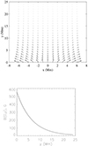 |
Fig. 1. Upper panel: Magnetic field vectors at the initial state obtained with the flux function A(x, y). Bottom panel: Dependence of the magnetic field B(0, y) on height y. |
To set the realistic physical parameters of the stratified solar atmosphere, we used the model proposed by Avrett & Loeser (2008). The temperature, density, Alfvén, and sound speed profiles are presented in Fig. 2. We note that the propagation time of Alfvén waves from the corona to the transition region is less than a few seconds due to the large value of the Alfvén speed in the corona,  Mm/s. Meanwhile, according to the estimates made by Tsap & Kopylova (2024), the propagation time of Alfvén waves in the WKB approximation from the transition region to the photosphere can reach several minutes.
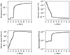 |
Fig. 2. Dependence of temperature, density, Alfvén, and sound velocities on height y at x = 0 according to the solar atmosphere model of Avrett & Loeser (2008) and the adopted magnetic configuration. |
The Alfvén pulse of transverse velocity at time t = 0 is given as (e.g., Jelínek et al. 2020)
 (13)
(13)
Here, A0 is the pulse amplitude, ω = 0.1 Mm is the pulse width, x0 = 1 Mm, and y0 = 5 Mm (see Fig. 3).
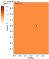 |
Fig. 3. Sketch of the initial velocity distribution Vz (Mm/s) at t = 0 s (see Eq. 13), located at x0 = 1 Mm and y0 = 5 Mm. The velocity pulse values are shown in white and brown. |
Proceeding from the above, we can conclude that the components of the velocity Vz(x, y) and the magnetic field Bz(x, y) are directed perpendicular to the plane. It suggests that we used 2.5D numerical model setup.
We applied the PLUTO code to provide the numerical simulation (Mignone et al. 2007, 2012). PLUTO numerically solves the systems of partial differential equations for different astronomical tasks. It allows one to use different numerical algorithms that can be combined to solve systems of conservation laws based on Godunov-type schemes.
3. Results of numerical simulation
The initial velocity disturbance (see Eq. 13) is presented in Fig. 3. As can be seen, the initial perturbation resembles torsional oscillations because the perturbed velocity Vz has a different direction at x < 1 Mm and x > 1 Mm. We note that the initial characteristic value of the velocity disturbance |Vz(t = 0)| ≈ 3.3 Mm/s is comparable to the local Alfvén velocity VA(0, 10) (see Fig. 2). This suggests that non-linear effects play an important role during wave generation and propagation.
The evolution of the energy flux with the initial velocity pulse Vz is partially shown in Fig. 4. The position of the energy flux maximum Sy is represented by the white contours (panels a–c) and the red contour (panel d). As shown, the energy fluxes begin to propagate in opposite directions along the magnetic field lines at t = 1 s. The energy flux reaches the transition region at t = 7 s, where a significant part of the flux is reflected and propagates upwards (Fig. 4 panels b and c). We observed wave reflection throughout the simulation. The maximum energy flux reaches the photosphere and is reflected at t = 120 s (Fig. 4, panel d). An essential weakening of the flux in the dense layers of the lower chromosphere and photosphere can be seen from the changes in the flux values indicated by the colour bars. According to our calculations, at the start of the simulation, the value of the energy flux was Sy ∼ 109 W/m2. When the flux maximum reaches the photosphere (temperature minimum region), it decreases to a value of Sy ∼ 6 × 10⁵ W/m2, which is at least one order of magnitude lower than the energy flux required (∼107 W/m2) to produce the optical emission observed from large solar flares (Russell & Fletcher 2013).
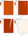 |
Fig. 4. Snapshots of the energy flux at t = 1 (a), t = 7 s (b), t = 20 s (c), and t = 120 s (d) at the start of the simulation. Contours illustrate the evolution of the disturbance during propagation. White and red contours show the location of the energy flux maximum, which propagates downwards. The black contour shows the energy flux that propagates upwards. |
To obtain the characteristic wave period produced by the pulse, we analysed variations in the velocity component Vx. The time series were produced at the coordinates [x, y]=[0.5, 0.1] Mm. We applied the wavelet transform (Torrence & Compo 1998) to study quasi-periodic variations in Vx.
As shown in Fig. 5, the wavelet spectrum contains variations with a characteristic period of Tp ∼ 10 s. This suggests that the propagation time is not determined by dissipation in the chromosphere (De Pontieu et al. 2001; Leake et al. 2005; Zaqarashvili et al. 2013; Soler et al. 2017), since the damping of Alfvén waves strongly depends on a wave period.
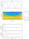 |
Fig. 5. Upper panel: (a) Time series of the velocity component variations Vx at y = 0.1 Mm. Time t = 0 corresponds to t = 60 s after the start of the simulation. (b) Wavelet power spectrum of the Vx time series. The solid line is the cone of influence. (c) Global wavelet power spectrum with a confidence level of 95% marked by the dashed red line. Bottom panel: Comparison of time series of variations in the velocity component, Vx at y = 3 Mm, 1 Mm. |
The bottom panel of Fig. 5 shows a comparison of Vx variations at points with coordinates [x, y]=[0.5, 3] Mm and [x, y]=[0.5, 1] Mm. As shown, the influence of non-linear effects is greater at high altitudes and decreases as the disturbance reaches the photosphere, where stratification contributes more significantly to the nature of waves propagation.
We calculated the distribution of the propagation velocity of the maximum energy flux Vpr with height y. A comparison between the Alfvén velocity VA, sound speed cs, and Vpr is presented in Fig. 6. The velocity Vpr is significantly lower in the corona and chromosphere than VA, but this difference becomes small in the photosphere. On the other hand, Vpr > cs in the corona, and Vpr ≈ VA at an altitude of ∼500 km. This circumstance can be associated with two phenomena. First, the difference in propagation times can be caused by non-linear effects. Second, atmospheric stratification can lead to a decrease in group (propagation) velocity even for linear Alfvén waves. This suggests that the differences observed between the propagation velocity and the Alfvén velocity are due to both non-linear effects and atmospheric stratification. According to Tsap et al. (2020), the stratification becomes important if

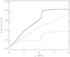 |
Fig. 6. Dependence of the Alfvén velocity VA (solid line), the propagation velocity Vpr of the energy flux maximum (dashed line), and the sound speed cs (dashed-dotted line) on height, obtained from the simulation. |
Adopting Tp = 10 s, VA = 10−2 − 10−1 Mm/s, and H = 0.2 Mm, we find that the latter inequality is well satisfied for the adopted model of the solar chromosphere and the magnetic configuration. In the photosphere, VA is small; therefore, the inequality is poorly satisfied, and the value of Vpr should be close to the group velocity VA, as in the case of the WKB approximation (Fig. 6).
To estimate the propagation time of the energy flux τ(y), we used (e.g. Tsap & Kopylova 2024)
 (14)
(14)
where Vpr represents the propagation velocity.
The dependence τ(y) obtained with Eq. (14) is presented in Fig. 7, which presents a comparison of propagation times obtained with the WKB approximation and the numerical simulation. As shown, the considered propagation times are comparable; that is, the total propagation times do not differ and are determined by the propagation of Alfvén waves originating from heights of ∼1 Mm, where the wave amplitude is expected to be quite small. This suggests that the main reason for the difference in propagation time is atmospheric stratification. However, it is not possible to clearly separate non-linear or transition phenomena from the effects related to plasma inhomogeneity.
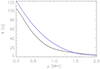 |
Fig. 7. Propagation time τ of Alfvén waves with height calculated in the WKB approximation (black line) and propagation time of the Alfvén pulse obtained from the model results (blue line). |
4. Conclusions and discussion
We performed a numerical simulation of a large-amplitude Alfvén pulse propagating from the solar corona to the photosphere, based on the system of ideal MHD equations. The Alfvén velocity pulse was specified perpendicular to the magnetic field lines as given by Eq. (13). The equilibrium magnetic configuration was described by the flux function A(x, y) according to Eq. (9). The magnetic field reached values ≈110 G and ≈550 G in the solar corona and photosphere, respectively.
The propagation time of the Alfvén energy flux maximum from the corona to the photosphere obtained through the model is τ ≈ 120 s. This time appears to be quite long compared to the characteristic values observed with ASO-S in the white-light solar flares that are inferred from the time delays between hard X-ray and optical emission (∼1 min), as proposed by Jing et al. (2024). In this context, we note that the propagation velocity of the maximum energy flux is significantly lower than the local Alfvén velocity in the solar corona and chromosphere. We associate this phenomenon with the wave non-linearity and the stratification of the solar atmosphere. However, we are unable to determine the relative role of these processes in the behavior of Alfvén-type waves.
We also note that the initial pulse width in the solar corona was about 100 km for the following reasons: The hydrodynamic description of the physical process is applicable if the characteristic frequency of the process Ω is significantly less than the effective collision frequency of the particles ν (i.e. Ω ≪ ν). The characteristic time is given by τi ∼ s/VTi, where VTi is the thermal ion velocity and s is the characteristic length of the system. Therefore, the characteristic frequency is Ω ∼ 1/τi ∼ VTi/s, and the condition Ω ≪ ν is satisfied if the mean free path of the particles is l ≪ s. According to the solar atmosphere model proposed by Avrett & Loeser (2008) based on the calculation formula proposed by Benz (1993), the mean free path of ions in the corona at an altitude of 5 Mm is l ∼ 30 km. This means that the MHD approximation is not valid if the characteristic pulse width is ω < 30 km. Therefore, we adopted a minimum initial pulse width of 100 km. Despite this, we find that the characteristic wave periods are ∼10 s, according to the wavelet analysis. We note that waves with periods of Tp ≲ 1 s strongly dissipate in the chromosphere due to ion-neutral collisions (De Pontieu et al. 2001; Leake et al. 2005; Zaqarashvili et al. 2013; Soler et al. 2017).
We showed that the wave energy flux significantly decreases in the course of propagation from the corona to the photosphere because of the non-linear effects and the stratification of the solar atmosphere. According to our estimates, the wave energy flux in the solar photosphere does not exceed ∼6 × 10⁵ W/m2. This is significantly lower than the required value of ∼107 W/m2 (Russell & Fletcher 2013). We can conclude that the contribution of Alfvén-type waves generated in the corona to the heating of the solar photosphere should be small. On the other hand, these modes can effectively heat the solar chromosphere, which may contribute significantly to the optical emission of solar flares (e.g. Russell & Stackhouse 2013; Kerr et al. 2016; Reep & Russell 2016; Reep et al. 2018). We also do not exclude an important role for other mechanisms of photosphere heating (e.g. heating in situ).
Acknowledgments
This research was partially supported by the Ministry of Science, Technological Development and Innovation of the Republic of Serbia (MSTDIRS) through contract number 451-03-136/2025-03/200002 made with Astronomical Observatory (Belgrade) (I. Zhivanovich), as well as, by the Ministry of Science and Higher Education, research work No. 122022400224-7 (V.V. Smirnova), and by a grant from the Russian Science Foundation project no. 22-12-00308-P (Yu.T. Tsap).
References
- Alfvén, H. 1942, Nature, 150, 405 [Google Scholar]
- Allred, J. C., Kowalski, A. F., & Carlsson, M. 2015, ApJ, 809, 104 [NASA ADS] [CrossRef] [Google Scholar]
- Avrett, E. H., & Loeser, R. 2008, ApJS, 175, 229 [Google Scholar]
- Belcher, J. W., & Davis, L. 1971, J. Geophys. Res., 76, 3534 [Google Scholar]
- Benz, A. O. 1993, Plasma Astrophysics: Kinetic Processes in Solar and Stellar Coronae (Dordrecht: Kluwer) [CrossRef] [Google Scholar]
- Boyer, R., Sotirovsky, P., Machado, M. E., & Rust, D. M. 1985, Sol. Phys., 98, 255 [Google Scholar]
- Brady, C. S., & Arber, T. D. 2016, ApJ, 829, 80 [Google Scholar]
- Carlsson, M., Hansteen, V. H., de Pontieu, B., et al. 2007, PASJ, 59, S663 [Google Scholar]
- Chmielewski, P., Srivastava, A. K., Murawski, K., & Musielak, Z. E. 2013, MNRAS, 428, 40 [Google Scholar]
- De Pontieu, B., Martens, P. C. H., & Hudson, H. S. 2001, ApJ, 558, 859 [Google Scholar]
- De Pontieu, B., McIntosh, S. W., Carlsson, M., et al. 2007, Science, 318, 1574 [Google Scholar]
- Emslie, A. G., & Sturrock, P. A. 1982, Sol. Phys., 80, 99 [Google Scholar]
- Fletcher, L., & Hudson, H. S. 2008, ApJ, 675, 1645 [Google Scholar]
- Gan, W., Zhu, C., Deng, Y., et al. 2023, Sol. Phys., 298, 68 [NASA ADS] [CrossRef] [Google Scholar]
- Goossens, M. L., Arregui, I., & Van Doorsselaere, T. 2019, Front. Astron. Space Sci., 6, 20 [Google Scholar]
- Hollweg, J. V. 1982, ApJ, 257, 345 [NASA ADS] [CrossRef] [Google Scholar]
- Jelínek, P., Karlický, M., Smirnova, V. V., & Solov’ev, A. A. 2020, A&A, 637, A42 [NASA ADS] [CrossRef] [EDP Sciences] [Google Scholar]
- Jess, D. B., Mathioudakis, M., Erdélyi, R., et al. 2009, Science, 323, 1582 [Google Scholar]
- Jing, Z., Li, Y., Feng, L., et al. 2024, Sol. Phys., 299, 11 [Google Scholar]
- Jurčák, J., Kašparová, J., Švanda, M., & Kleint, L. 2018, A&A, 620, A183 [NASA ADS] [CrossRef] [EDP Sciences] [Google Scholar]
- Kerr, G. S. 2022, Front. Astron. Space Sci., 9, 1060856 [NASA ADS] [CrossRef] [Google Scholar]
- Kerr, G. S., Fletcher, L., Russell, A. J. B., & Allred, J. C. 2016, ApJ, 827, 101 [NASA ADS] [Google Scholar]
- Kretzschmar, M. 2011, A&A, 530, A84 [NASA ADS] [CrossRef] [EDP Sciences] [Google Scholar]
- Kudoh, T., & Shibata, K. 1999, ApJ, 514, 493 [NASA ADS] [CrossRef] [Google Scholar]
- Kuźma, B., Murawski, K., & Poedts, S. 2021, MNRAS, 506, 989 [CrossRef] [Google Scholar]
- Leake, J. E., Arber, T. D., & Khodachenko, M. L. 2005, A&A, 442, 1091 [NASA ADS] [CrossRef] [EDP Sciences] [Google Scholar]
- Machado, M. E., Avrett, E. H., Vernazza, J. E., & Noyes, R. W. 1980, ApJ, 242, 336 [NASA ADS] [CrossRef] [Google Scholar]
- Machado, M. E., Emslie, A. G., & Avrett, E. H. 1989, Sol. Phys., 124, 303 [NASA ADS] [CrossRef] [Google Scholar]
- Martínez Oliveros, J.-C., Hudson, H. S., Hurford, G. J., et al. 2012, ApJ, 753, L26 [CrossRef] [Google Scholar]
- Mathioudakis, M., Jess, D. B., & Erdélyi, R. 2013, Space Sci. Rev., 175, 1 [Google Scholar]
- McIntosh, S. W., de Pontieu, B., Carlsson, M., et al. 2011, Nature, 475, 477 [Google Scholar]
- Mignone, A., Bodo, G., Massaglia, S., et al. 2007, ApJS, 170, 228 [Google Scholar]
- Mignone, A., Zanni, C., Tzeferacos, P., et al. 2012, ApJS, 198, 7 [Google Scholar]
- Morton, R. J., Sharma, R., Tajfirouze, E., & Miriyala, H. 2023, Rev. Mod. Plasma Phys., 7, 17 [NASA ADS] [CrossRef] [Google Scholar]
- Murawski, K., Solov’ev, A., Musielak, Z. E., Srivastava, A. K., & Kraśkiewicz, J. 2015, A&A, 577, A126 [NASA ADS] [CrossRef] [EDP Sciences] [Google Scholar]
- Neidig, D. F. 1989, Sol. Phys., 121, 261 [NASA ADS] [CrossRef] [Google Scholar]
- Nishizuka, N., Shimizu, M., Nakamura, T., et al. 2008, ApJ, 683, L83 [NASA ADS] [CrossRef] [Google Scholar]
- Priest, E. R. 1982, Solar Magneto-Hydrodynamics (Dordrecht: D. Reidel) [CrossRef] [Google Scholar]
- Procházka, O., Milligan, R. O., Allred, J. C., et al. 2017, ApJ, 837, 46 [Google Scholar]
- Reep, J. W., & Russell, A. J. B. 2016, ApJ, 818, L20 [Google Scholar]
- Reep, J. W., Russell, A. J. B., Tarr, L. A., & Leake, J. E. 2018, ApJ, 853, 101 [NASA ADS] [CrossRef] [Google Scholar]
- Russell, A. J. B. 2018, Sol. Phys., 293, 83 [Google Scholar]
- Russell, A. J. B., & Fletcher, L. 2013, ApJ, 765, 81 [Google Scholar]
- Russell, A. J. B., & Stackhouse, D. J. 2013, A&A, 558, A76 [NASA ADS] [CrossRef] [EDP Sciences] [Google Scholar]
- Sadykov, V. M., Stefan, J. T., Kosovichev, A. G., et al. 2024, ApJ, 960, 80 [Google Scholar]
- Singh, B., Srivastava, A. K., Sharma, K., Mishra, S. K., & Dwivedi, B. N. 2022, MNRAS, 511, 4134 [NASA ADS] [CrossRef] [Google Scholar]
- Soler, R., Terradas, J., Oliver, R., & Ballester, J. L. 2017, ApJ, 840, 20 [Google Scholar]
- Srivastava, A. K., Singh, A., Singh, B., et al. 2024, Philosoph. Trans. Roy. Soc. A, 382, 20230220 [Google Scholar]
- Terradas, J., Oliver, R., Ballester, J. L., & Keppens, R. 2008, ApJ, 675, 875 [Google Scholar]
- Thurgood, J. O., & McLaughlin, J. A. 2013, Sol. Phys., 288, 205 [NASA ADS] [CrossRef] [Google Scholar]
- Tomczyk, S., McIntosh, S. W., Keil, S. L., et al. 2007, Science, 317, 1192 [Google Scholar]
- Torrence, C., & Compo, G. P. 1998, Bull. Am. Meteorol. Soc., 79, 61 [Google Scholar]
- Tsap, Y., & Kopylova, Y. 2021, Sol. Phys., 296, 5 [NASA ADS] [CrossRef] [Google Scholar]
- Tsap, Y. T., & Kopylova, Y. G. 2024, Geomagn. Aeron., 63, 1086 [Google Scholar]
- Tsap, Y. T., & Stepanov, A. V. 2008, Astron. Lett., 34, 52 [Google Scholar]
- Tsap, Y. T., Stepanov, A. V., Kopylova, Y. G., & Khaneichuk, O. V. 2020, Geomagn. Aeron., 60, 446 [Google Scholar]
- Watanabe, K., Shimizu, T., Masuda, S., Ichimoto, K., & Ohno, M. 2013, ApJ, 776, 123 [NASA ADS] [CrossRef] [Google Scholar]
- Wójcik, D., Kuźma, B., Murawski, K., & Musielak, Z. E. 2020, A&A, 635, A28 [NASA ADS] [CrossRef] [EDP Sciences] [Google Scholar]
- Yang, L., & Chao, J. K. 2013, Chin. J. Space Sci., 33, 353 [Google Scholar]
- Zaqarashvili, T. V., Khodachenko, M. L., & Soler, R. 2013, A&A, 549, A113 [NASA ADS] [CrossRef] [EDP Sciences] [Google Scholar]
All Figures
|
Fig. 1. Upper panel: Magnetic field vectors at the initial state obtained with the flux function A(x, y). Bottom panel: Dependence of the magnetic field B(0, y) on height y. |
| In the text | |
|
Fig. 2. Dependence of temperature, density, Alfvén, and sound velocities on height y at x = 0 according to the solar atmosphere model of Avrett & Loeser (2008) and the adopted magnetic configuration. |
| In the text | |
|
Fig. 3. Sketch of the initial velocity distribution Vz (Mm/s) at t = 0 s (see Eq. 13), located at x0 = 1 Mm and y0 = 5 Mm. The velocity pulse values are shown in white and brown. |
| In the text | |
|
Fig. 4. Snapshots of the energy flux at t = 1 (a), t = 7 s (b), t = 20 s (c), and t = 120 s (d) at the start of the simulation. Contours illustrate the evolution of the disturbance during propagation. White and red contours show the location of the energy flux maximum, which propagates downwards. The black contour shows the energy flux that propagates upwards. |
| In the text | |
|
Fig. 5. Upper panel: (a) Time series of the velocity component variations Vx at y = 0.1 Mm. Time t = 0 corresponds to t = 60 s after the start of the simulation. (b) Wavelet power spectrum of the Vx time series. The solid line is the cone of influence. (c) Global wavelet power spectrum with a confidence level of 95% marked by the dashed red line. Bottom panel: Comparison of time series of variations in the velocity component, Vx at y = 3 Mm, 1 Mm. |
| In the text | |
|
Fig. 6. Dependence of the Alfvén velocity VA (solid line), the propagation velocity Vpr of the energy flux maximum (dashed line), and the sound speed cs (dashed-dotted line) on height, obtained from the simulation. |
| In the text | |
|
Fig. 7. Propagation time τ of Alfvén waves with height calculated in the WKB approximation (black line) and propagation time of the Alfvén pulse obtained from the model results (blue line). |
| In the text | |
Current usage metrics show cumulative count of Article Views (full-text article views including HTML views, PDF and ePub downloads, according to the available data) and Abstracts Views on Vision4Press platform.
Data correspond to usage on the plateform after 2015. The current usage metrics is available 48-96 hours after online publication and is updated daily on week days.
Initial download of the metrics may take a while.