| Issue |
A&A
Volume 691, November 2024
|
|
|---|---|---|
| Article Number | A55 | |
| Number of page(s) | 12 | |
| Section | The Sun and the Heliosphere | |
| DOI | https://doi.org/10.1051/0004-6361/202451507 | |
| Published online | 30 October 2024 | |
Effects of field line expansion on Alfvén waves and vortices
Department of Physics, University of Aberystwyth, Aberystwyth SY23 3BZ, Wales, UK
Received:
15
July
2024
Accepted:
24
September
2024
Abstract
Context. Simulations and observations of the solar atmosphere often reveal the presence of torsional Alfvén waves and vortices with sufficient power to heat the solar corona and accelerate the solar wind.
Aims. We challenge the long-held view that low-frequency Alfvén waves are suppressed due to inhomogeneities and steep spatial gradients in the atmosphere. Alfvén waves and vortices in a stratified solar atmosphere are modelled with the aim of calculating and comparing their energy flux for different field line geometries.
Methods. We show that the general problem of linear Alfvén wave propagation along field lines of arbitrary geometry can be reduced to a set of Klein–Gordon equations for the perturbations of the magnetic field and velocity. Solutions and corresponding energy fluxes are constructed for three cases with different expansion rates of the field lines in the lower atmosphere.
Results. Expansion rates that are associated with cut-off free propagation in the lower atmosphere suppress the perturbation amplitudes and the corresponding energy flux. These include the uniform field model and the thin flux tube model. A counterexample with an intermediate field line expansion rate and non-vanishing cut-offs exhibits consistently large perturbation amplitudes and unrestricted energy flux across the entire frequency spectrum.
Conclusions. Field lines with different expansion rates and geometries in the lower atmosphere can significantly alter the amplitudes of the Alfvén waves and vortices and the extent of the energy flux entering the corona.
Key words: magnetohydrodynamics (MHD) / waves / methods: analytical / Sun: atmosphere / Sun: magnetic fields
Corresponding author; This email address is being protected from spambots. You need JavaScript enabled to view it. .
© The Authors 2024
 Open Access article, published by EDP Sciences, under the terms of the Creative Commons Attribution License (https://creativecommons.org/licenses/by/4.0), which permits unrestricted use, distribution, and reproduction in any medium, provided the original work is properly cited.
This article is published in open access under the Subscribe to Open model. This email address is being protected from spambots. You need JavaScript enabled to view it. to support open access publication.
1. Introduction
Eighty years since their discovery (Alfvén 1942), Alfvén waves continue to attract much research interest from laboratory and space plasma physicists. The waves represent an interplay between plasma inertia and the tension of the magnetic field lines, similar to waves on a string instrument.
Alfvén waves have long been thought to be a possible candidate in resolving two major and longstanding problems in solar physics and astrophysics: the heating of the solar and stellar atmospheres and the acceleration of solar and stellar winds. The waves can be generated through random motions or magnetic reconnection in the photosphere and chromosphere.
The main reason why Alfvén waves have been favoured in comparison to other types of magnetohydrodynamic (MHD) waves is that incompressible Alfvénic disturbances travelling along magnetic field lines should be less susceptible to steepening and dissipation before reaching the upper atmosphere of the sun. They could therefore transport significant amounts of energy along the magnetic field that extends from the visible surface of the sun (photosphere) into the hot and tenuous atmosphere (corona) and further (Liu et al. 2019; Soler et al. 2019; Alielden & Taroyan 2022).
However, early studies by Ferraro (1954) and Ferraro & Plumpton (1958) indicated that the chromosphere and transition region between the photosphere and the corona should act as strong reflectors of wave energy due to steep temperature and density gradients. Follow-up theoretical modelling endorsed the view that Alfvén waves are attenuated by the abrupt increase in their propagation speed by more than a factor of 10 (over about 1 Mm) in passing from the chromosphere to the corona (An et al. 1989; Parker 1991).
The reflection is especially strong at long periods. On the other hand, Alfvén waves with shorter periods are efficiently damped in the chromosphere by a variety of mechanisms, for example by ion-neutral collisions (Zaqarashvili et al. 2013).
These views have been challenged in the new era of solar observations. High-resolution spectroscopic observations with Hinode/EIS, SST, IRIS, and other instruments have demonstrated the ubiquity of Alfvén waves in the solar atmosphere.
Large-amplitude magnetic twists and Alfvénic waves appear to be propagating along different magnetic structures carrying significant amounts of energy into the chromosphere and the corona (Jess et al. 2009; McIntosh et al. 2011; De Pontieu et al. 2014). Recent work has revealed and characterised ubiquitous and continuous wave activity in extreme ultraviolet image time series through the application of a novel method (Morgan & Korsós 2022).
Several studies have proposed that the reflection may lead to resonances, and thus to a very large energy flux at those frequencies (Hollweg 1978, 1984; Matsumoto & Shibata 2010). However, Leer et al. (1982) pointed out that such large energy fluxes can only be produced if the wave-driver matches the nodes of the resonator and remains phase-coherent over many wave periods. In addition, the resonator should remain fixed in time over many wave periods. These requirements impose strong restrictions on the transport of large amounts of energy from the photosphere to the corona through resonances.
Studies carried out by Wedemeyer-Böhm et al. (2012), Battaglia et al. (2021), Breu et al. (2023), and Silva et al. (2024) show the presence of ubiquitous vortical or swirling motions both in observations and numerical simulations. These events are correlated with perturbations of the magnetic field. At photospheric and chromospheric levels, they form Alfvén pulses that propagate upward and may contribute to chromospheric heating. Energy is transported following a vortical motion.
Theoretical modelling of Alfvén wave propagation has traditionally been carried out in standard magnetic field geometries. These include a uniform field or a thin flux tube whereby the tube thickness is small compared with the characteristic scale of the magnetic field variation. However, the magnetic field lines can expand in different ways as the density drops from the photosphere to the corona. In general, the shape of the field lines can be determined from a divergence-free condition in curvilinear coordinates (Taroyan et al. 2021).
Here we demonstrate that the above-mentioned standard geometries inhibit the flux of Alfvén wave energy into the upper atmosphere. Examples of structures with such geometries are a stratified atmosphere with a uniform magnetic field, a radially expanding magnetic field, or a thin flux tube. Reflection approaches 100% at low frequencies. We show that the wave reflection strongly depends on the magnetic field geometry and that it may vanish in certain cases, resulting in very efficient transport of Alfvén wave energy into the upper atmosphere.
The paper is structured as follows. Section 2 summarises some important results for thin flux tubes in a cylindrical coordinate system. In Sect. 3 we demonstrate that the problem of Alfvén wave propagation in a general field line geometry can be reduced to a set of Klein–Gordon equations in local curvilinear coordinates. Three different cases of field line expansion rates in the lower atmosphere are introduced and compared in Sect. 4; the corresponding Alfvén wave variables are derived in Sect. 5 and compared in Sect. 6. The wave energy fluxes associated with the three cases are derived and compared in Sect. 7. Section 8 summarises the presented results and draws our overall conclusions.
2. Alfvén waves on thin flux tubes
Models of Alfvén wave propagation on thin flux tubes are based on the well-known relationship (9) between the background magnetic field and the tube cross-section (Hollweg et al. 1982). Studies carried out in this approximation show that Alfvén waves are strongly reflected by density and temperature gradients especially at low frequencies (An et al. 1989; Murawski & Musielak 2010; Soler et al. 2017; Tsap & Kopylova 2021). Therefore, very little wave energy is available at coronal heights.
The relationship between the background field and the cross-sectional radius (9) permits a wide range of thin flux tubes with different variations in the tube cross-section. It also includes the case of a uniform field with vertical field lines. The propagation and reflection of Alfvén waves in an atmosphere with a uniform field has been studied since Ferraro (1954) and Ferraro & Plumpton (1958). The wave behaviour in a uniform field is similar to the results obtained for a thin flux tube.
The thin flux tube approximation considers field lines close to the tube’s vertical axis of symmetry, where the radial component, Br, vanishes. On field lines near the tube axis we can Taylor expand Br with respect to r,
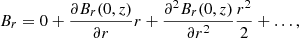 (1)
(1)
where z is the vertical coordinate. Dividing by r and ignoring terms of order r, we obtain
 (2)
(2)
The derivative of Br can be Taylor expanded in a similar way:
 (3)
(3)
Ignoring terms of order r in expansion (3) and combining it with expression (2), we obtain
 (4)
(4)
The divergence-free condition in cylindrical coordinates reads
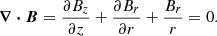 (5)
(5)
For field lines near the axis of symmetry we apply the obtained relationship (4), to rewrite the divergence-free condition in the following form:
 (6)
(6)
Along the field lines the following relationship is satisfied:
 (7)
(7)
Using the obtained Eq. (6) for field lines close to the symmetry axis, we have
 (8)
(8)
Integrating Eq. (8) along an arbitrary field line, we obtain the condition of flux conservation for a thin flux tube:
 (9)
(9)
The above condition (9) can be derived in different ways. For example, in the case of a potential field, the flux function is conserved along the field lines, and it reduces to the left-hand side of (9) for field lines close enough to the symmetry axis (Ruderman et al. 2008; Verth et al. 2010; Soler et al. 2017). Condition (9) has been extensively used in studies of Alfvén waves on thin flux tubes.
The governing equation for the Alfvén waves on thin flux tubes can be written in the form of a Bessel equation, with a general solution in terms of the Hankel functions (see e.g. Hollweg (1978)):
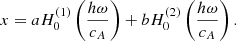 (10)
(10)
Here x = vφ/r, and cA = cA0exp(z/h) is the exponentially increasing Alfvén speed with a scale height h. The general solution (10) is derived assuming condition (9) is satisfied. In the case of an atmosphere with a uniform magnetic field and an exponential Alfvén speed, the governing equations are reduced to the wave equation, which, in turn, can be reduced to the Bessel equation, and the general solution is given by the same formula (10) (Hollweg 1978; Verth et al. 2010; Tsap & Kopylova 2021).
The model with an exponentially increasing Alfvén speed has been used to investigate the propagation of Alfvén waves in stellar atmospheres since Ferraro (1954). Ferraro & Plumpton (1958) expressed the solutions in terms of Bessel functions of the first and second kind of order zero. Cally (2012) pointed out that dropping the Bessel function Y0 used by Ferraro & Plumpton (1958) and An et al. (1989), among others, leads to unphysical reflection at infinity. Therefore, solutions are usually expressed in terms of the Hankel functions (10) that represent upgoing and downgoing waves, respectively.
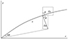 |
Fig. 1. Axisymmetric poloidal magnetic field described by cylindrical coordinates and local orthogonal curvilinear coordinates. The angle ϕ representing the angle of rotation around the vertical symmetry axis, z, is not shown. The figure shows distance, s, along a curved magnetic field; the angle, θ, between the poloidal field and the vertical axis; and incremental increases δs and δa, along and across the poloidal field, respectively. |
3. Klein–Gordon equations for Alfvén waves
In cylindrical coordinates (r, ϕ, z) axisymmetric motions are characterised by the condition ∂/∂ϕ = 0. We introduced local orthogonal curvilinear coordinates (a, ϕ, s) along a given magnetic field line tailored to the geometry of the magnetic field. Figure 1 shows that s is a curvilinear coordinate because it follows the curved path of the magnetic field line rather than a straight line. The coordinate s measures distance along the poloidal field line, and a is the distance perpendicular to the poloidal field line. The angle of rotation, ϕ, around the vertical z-axis is not shown. The magnetic field may be decomposed either into cylindrical components (Br, Bϕ, Bz) or into toroidal and poloidal components (0, Bϕ, Bs), where Bs denotes the poloidal field and there is no component in the transverse direction, a.
The propagation of axisymmetric Alfvén waves in general field geometries can be studied using the equations of motion and induction in local curvilinear coordinates (Hollweg et al. 1982; Taroyan et al. 2021):
 (11)
(11)
Here Bs is the time-independent background magnetic field and s is the local curvilinear coordinate along a given field line.
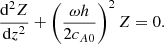
It is well known that one-dimensional wave propagation in the presence of gravity typically gives rise to the Klein–Gordon equation and with it the introduction of a cut-off frequency (Roberts 2004; Taroyan & Erdélyi 2008). The cut-off frequency is related to the scale-height, which is a measure of the strength of gravity. The significance of the Klein–Gordon equation is that it introduces a timescale imposed by the equilibrium. For a Klein–Gordon equation with constant coefficients, wave propagation occurs only for frequencies above the cut-off frequency. Frequencies below this value result in no propagation and the motion is evanescent (Roberts 2004).
Noble et al. (2003) derived a Klein–Gordon equation for the velocity perturbation, Vφ, and Routh et al. (2020) show that the magnetic field perturbation, Bφ, is determined from the Klein–Gordon equation. These studies are carried out under the assumption of a thin flux tube approximation (i.e. the condition of flux conservation (9) is satisfied).
Here we show that the general problem of Alfvén wave propagation along field lines of arbitrary geometry can be reduced to a set of Klein–Gordon equations for the perturbations of the magnetic field, Bφ, and the velocity, Vφ. This approach allows us to explore the relationship between the waves, the corresponding energy fluxes, and the cut-off frequencies for different geometries.
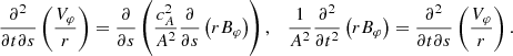
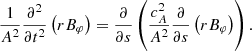
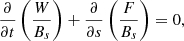
Firstly, we differentiate the momentum and the induction Equation (11) with respect to t and s, respectively, to obtain
 (12)
(12)
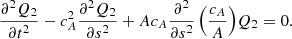
Equation (12) can be combined to eliminate the variable Bφ
 (13)
(13)
where  and A2 = Bsr2. By introducing the variable
  , we reduce the right-hand side of Eq. (13) to
 (14)
(14)
Equation (13) is therefore reduced to a Klein–Gordon equation:
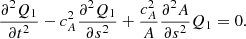 (15)
(15)
The second Klein–Gordon equation can be derived in a similar way. We differentiate the momentum and the induction Equation (11) with respect to s and t, respectively, to obtain
 (16)
(16)
Equation (16) can be combined to eliminate the variable Vφ:
 (17)
(17)
By introducing the variable  , we reduce the right-hand side of Eq. (17) to
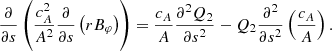 (18)
(18)
Equation (17) is therefore reduced to a Klein–Gordon equation of the form
 (19)
(19)
In summary, we have demonstrated that the propagation of Alfvén waves along field lines of arbitrary geometry is determined by the Klein–Gordon equation
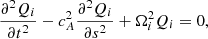 (20)
(20)
where s is the coordinate along the poloidal field, cA is the Alfvén speed,
 (21)
(21)
is the wave variable, A2 = Bsr2, and
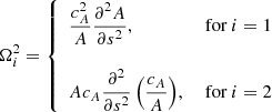 (22)
(22)
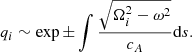
is the square of the cut-off frequency.
By setting Qi = qiexp(iωt), we can reduce the Klein–Gordon Eq. (20) to the following form:
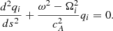 (23)
(23)
In the WKB approximation, eigenfrequencies below the cut-off, ω < Ωi, correspond to growing and decaying solutions, whereas those above the cut-off, ω > Ωi, correspond to propagating solutions.
The thin flux tube approximation represents a particular case of a general class of field lines that can be self-consistently determined using the solenoidal condition in curvilinear coordinates (Taroyan et al. 2021). Here we show that the commonly used models, including the thin flux tube, correspond to a degeneracy in the Klein–Gordon Eq. (20), which has important implications.
For field lines close to the symmetry axis we have Br ≪ Bz so that Bs ≈ Bz. The conservation of magnetic flux for thin flux tubes (9) is then reduced to A2 = Bsr2 ≈ Bzr2= const along the field lines.
Therefore, the thin flux tube approximation assumes A= const along the poloidal field, in which case the cut-off frequency Ω1 vanishes. It is important to note that this result is true for all thin flux tubes regardless of the particular field line geometry.
The condition A= const remains true for the cases of a uniform field and a radially expanding field. Therefore, the cut-off frequency vanishes (Ω1 = 0) and the corresponding Klein–Gordon equation again becomes degenerate.
Below we demonstrate that vanishing cut-off frequencies (cases I and II) strongly restrict the wave energy flux into the upper atmosphere. A counterexample (case III) shows that more generally (i.e. in non-degenerate cases) the transport of the wave energy by Alfvén waves into the corona can be much more efficient.
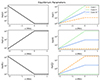 |
Fig. 2. Equilibrium parameters in the atmosphere. The panels on the left display the variation of density, Alfvén speed and magnetic field. The panels on the right show the radial distance, r = r(s), and the corresponding parameters that determine the cut-off frequencies Ω1 and Ω2. Logarithmic scales are used. |
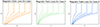 |
Fig. 3. Geometry of the magnetic field in the r − z plane. The field lines exponentially expand in the lower atmosphere and are vertical in the uniform upper atmosphere. |
4. The background atmosphere
Following previous studies, we split the atmosphere into two parts (e.g. Hollweg et al. 1982). The upper atmosphere is uniform and all the parameters here are constant. In the lower atmosphere, the Alfvén speed increases exponentially with height. In order to explore in more detail the behaviour of the waves and the role of the magnetic field geometry, we consider three different cases for the lower atmosphere that are summarised in Table 1.
The three cases.
Table 1 shows the variation of the Alfvén speed, density, magnetic field, and the radial distance in the lower atmosphere. All the parameters are treated as functions of the field line coordinate, s. The photosphere is located at s = −2 Mm, and the coronal base is located at s = 0 Mm. The subscript 0 indicates the values of the corresponding parameters at the coronal base, s = 0. Table 1 shows that all the parameters are the same for the three cases except the distance between the field line and the symmetry axis, r.
We assume that the density decreases from the photosphere to the base of the corona by eight orders of magnitude (Vernazza et al. 1981). Further, in agreement with the measurements, Table 1 suggests a magnetic field decrease by two orders of magnitude (Aschwanden 2019). The Alfvén speed should then increase by two orders of magnitude. The scale height corresponding to these variations is h = 869.5 km. The main difference between the three cases is the expansion factor of the field lines.
Observations suggest that magnetic flux tubes originating from concentrated sources in the photosphere can expand significantly, by a factor of 100 or more, as they rise to the corona (Gary 2001; Solanki et al. 2006). The cross-sectional area of these flux tubes increases due to the divergence of field lines (Aschwanden 2019). We consider three possibilities: the field lines expand by a factor of 10 in case I, a factor of 1000 in case II, and a factor of 100 in case III.
The parameter variations described above are visualised in Fig. 2. We note that logarithmic scales are used for the vertical axes. We adopt a two-layer model of the solar atmosphere with a constant scale height of less than 1 Mm in the lower layer and an infinite scale height corresponding to high temperatures in the upper layer (Leer et al. 1982; Hollweg 1984; Tsap & Kopylova 2021). The background atmosphere can be approximated more accurately. For example, Hollweg (1978) introduced a model with 16 exponential layers mimicking the Munro–Jackson model to study the behaviour of Alfvén waves from the lower atmosphere to the outer corona and their role in solar wind acceleration. However, the Klein–Gordon equations derived in the previous section do not assume any specific structure of the atmosphere. Therefore, we could argue that our main conclusions regarding the relationship between the cut-off frequencies, the field line geometry, and the energy flux carried by the Alfvén waves should remain valid for more complex structures.
Figure 2 shows that the atmosphere is split into a lower layer, s < 0, with an exponentially increasing Alfvén speed, density, and magnetic field, and an upper layer, s > 0, with a constant value for the same parameters. In agreement with previous studies, the solution in the infinite and constant upper layer is determined by an outgoing wave condition.
The panels on the right show the variations in the radial distance from the symmetry axis, r = r(s), and the parameters that determine the cut-off frequencies for the three cases. The parameter A is constant for case I (orange dashed line), and leads to a vanishing cut-off frequency Ω1. For case II (green dotted line) it is the parameter cA/A that remains constant, leading to vanishing cut-off frequency Ω2. For the case III (blue line) both cut-off frequencies remain different from 0.
Figure 3 displays the geometry of the magnetic field in arbitrary units. Equations (7) and (8) from Taroyan et al. (2021) establish relationships between the field components in local curvilinear and cylindrical coordinates. These relationships are used to construct and plot the field lines in the r − z plane. The axisymmetric geometry implies no dependence on the azimuthal angle ϕ.
The uniform field, Bs0, in the upper atmosphere, s > 0, corresponds to vertical field lines that are identical for the three cases. In the linear regime, the Alfvénic motions are decoupled from the other motions. However, the dynamic nature of the transition region or the inclination of the field lines in the upper atmosphere could play an important role as the waves become non-linear. The three cases show differences in the lower atmosphere, s < 0. In each case, the rate of the field line expansion is determined by the corresponding scale height: h for case I, h/3 for case II, and h/2 for case III. These three expansion rates result in very different wave behaviour.
The expressions from Table 1 show that the three cases have the same poloidal field, Bs, from the photospehre to the corona. These expressions and the relationships between the field components in local curvilinear and cylindrical coordinates can be used to determine the horizontal, r, and the vertical, z, components of the magnetic field. Figure 3 shows that Case I has the strongest horizontal component and the weakest vertical component at the photospheric level, s = −2 Mm, whereas case II has the strongest vertical component and the weakest horizontal component at the photospheric level.
5. Solutions of the Klein–Gordon equations
Using the equilibrium parameters introduced above, we derive and examine the solutions of the Klein–Gordon equations for the three cases. We first consider the two degenerate cases I and II that correspond to vanishing cut-off frequencies Ω1 and Ω2, respectively, in the Klein–Gordon equations. We then examine a counterexample (case III) where neither of the cut-off frequencies vanishes. The obtained results are then used to compare the magnetic field and velocity perturbations in the next section.
The solutions to the Klein–Gordon equations are constructed based on three key principles:
-
1.
The net wave energy flux is finite at all frequencies.
-
2.
The net wave energy flux is zero when the upgoing flux equals the downgoing flux.
-
3.
The upgoing flux from the photosphere is independent of the magnetic field geometry above and remains consistent across all three cases.
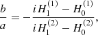
5.1. Case I
In the first case, which also includes thin flux tubes, we have the condition A = const, and the first cut-off frequency vanishes: Ω1 = 0. The corresponding Klein–Gordon equation for the lower atmosphere becomes degenerate. It is reduced to the wave equation with solutions that represent propagating waves.
The condition Ω1 = 0 holds for all thin flux tubes regardless of the particular dependence r = r(s) or cA = cA(s). In the lower atmosphere, s < 0, where the Alfvén speed increases exponentially with a scale height of h/2, the solutions are expressed in terms of the Hankel functions, similar to the expression (10) for cylindrical geometry:
 (24)
(24)
One difference between our solution (24) and the solution (10) used by Hollweg (1978) is the Alfvénic scale height: h/2 in (24) and h in (10). Another difference is the presence of an extra coefficient  in (24) in order to have physically acceptable solutions for all frequencies. We show in Sect. 7 that due to the coefficient
  there is no net energy flux when the upgoing and downgoing wave energy fluxes become equal to each other as ω → 0. On the other hand, the net flux remains finite as ω → ∞. The solution (24) is also applicable to a uniform or a radial magnetic field, where the same condition, A = const, is satisfied.
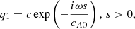
In addition to the variables qi, we introduce the new variables vφ and bφ: Vφ = vφexp(iωt), Bφ = bφexp(iωt). The velocity perturbation, vφ, can easily be found from the solution (24) and the relationship (21):
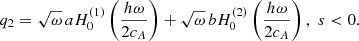
![Mathematical equation: $$ \begin{aligned} v_\varphi =\frac{i\sqrt{\omega }}{\sqrt{B_s}}\left[ a H_0^{(1)}\left(\frac{h\omega }{2c_{A}} \right) + b H_0^{(2)}\left(\frac{h\omega }{2c_{A}} \right)\right], \,\, s < 0. \end{aligned} $$](/articles/aa/full_html/2024/11/aa51507-24/aa51507-24-eq42.gif) (25)
(25)
The magnetic field perturbation, bφ, can be determined from the induction in Eq. (11):
 (26)
(26)
Using the obtained solution (24), the above expression is reduced to
![Mathematical equation: $$ \begin{aligned} b_\varphi =-\frac{i\sqrt{\omega B_s}}{c_{A}}\left[ a H_1^{(1)}\left(\frac{h\omega }{2c_{A}} \right) + b H_1^{(2)}\left(\frac{h\omega }{2c_{A}} \right)\right], \,\, s < 0. \end{aligned} $$](/articles/aa/full_html/2024/11/aa51507-24/aa51507-24-eq44.gif) (27)
(27)
The cut-off frequencies vanish in the upper atmosphere, and therefore only propagating waves can exist in this open region. Consistent with previous studies, we require the solution to represent an outgoing wave in the open region, s > 0,
 (28)
(28)
where cA0 = cA(s = 0) and c is the wave amplitude in the upper layer. The magnetic field and velocity perturbations, bφ and vφ, in the region s > 0 can be determined from expression (28):
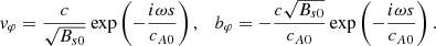 (29)
(29)
Here the index 0 indicates that the functions are evaluated at s = 0.
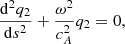
A relationship between the constant coefficients a and b can be established using the continuity of the magnetic field and the velocity perturbations across the interface at s = 0. The result is
 (30)
(30)
where the argument of the Hankel functions is at hω/(2cA0). Hollweg (1978) identified  as the ratio of downgoing energy flux to upgoing energy flux (see also Leer et al. (1982), Tsap & Kopylova (2021)).
5.2. Case II
For the second case we have cA/A= const along the field lines, corresponding to Ω2 = 0. Therefore, the second Klein–Gordon equation becomes degenerate. In the lower atmosphere, s < 0, the field lines expand with a scale height h/3, and the Alfvén speed increases with a scale height h/2. The equation for q2,
 (31)
(31)
is reduced to a Bessel equation with solutions similar to (24):
 (32)
(32)
Solutions of this type have been studied by Hollweg (1984), Cally (2012), and others in different contexts. Similarly to case I, the extra coefficient,  , ensures that there is no net flux of wave energy when the upgoing and downgoing fluxes balance each other (see Sect. 7). The net flux remains finite for all frequencies. The coefficients a and b are the same as in case I to satisfy the third principle (i.e. the upgoing flux from the photospehre remains independent of the magnetic field geometry above).
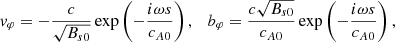
The magnetic field perturbation, bφ, in the lower atmosphere is expressed through Eq. (21):
![Mathematical equation: $$ \begin{aligned} b_\varphi =\frac{\sqrt{\omega B_s}}{c_{A}}\left[ a H_0^{(1)}\left(\frac{h\omega }{2c_{A}} \right) + b H_0^{(2)}\left(\frac{h\omega }{2c_{A}} \right)\right]. \end{aligned} $$](/articles/aa/full_html/2024/11/aa51507-24/aa51507-24-eq52.gif) (33)
(33)
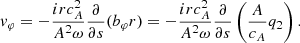
The velocity perturbation in the region s < 0 can be expressed using the equation of motion (11):
![Mathematical equation: $$ \begin{aligned} v_\varphi =-\frac{i c_{A} r}{A\omega }\frac{\mathrm{d} q_2}{\mathrm{d}s} =-\frac{i \sqrt{\omega }}{\sqrt{B_s}}\left[ a H_1^{(1)}\left(\frac{h\omega }{2c_{A}} \right) + b H_1^{(2)}\left(\frac{h\omega }{2c_{A}} \right)\right]. \end{aligned} $$](/articles/aa/full_html/2024/11/aa51507-24/aa51507-24-eq53.gif) (34)
(34)
Here we use the well-known differentiation rule for the Hankel functions: 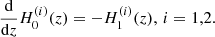
As in case I, we require the solution in the open and uniform region, s > 0, to represent an outgoing wave,
 (35)
(35)
where cA0 = cA(s = 0), and c is the constant amplitude in the upper layer.
The magnetic field and velocity perturbations, bφ and vφ in the region s > 0 can be determined from expression (35),
 (36)
(36)
where the index 0 indicates that the functions are evaluated at s = 0. The magnetic field and velocity perturbations, bφ and vφ, are continuous across the interface at s = 0,
![Mathematical equation: $$ \begin{aligned} a \sqrt{\omega }\,H_0^{(1)}+ b \sqrt{\omega }\,H_0^{(2)} = c, \, -i\sqrt{\omega }\left[a H_1^{(1)}+ b H_1^{(2)} \right] = -c, \end{aligned} $$](/articles/aa/full_html/2024/11/aa51507-24/aa51507-24-eq57.gif) (37)
(37)
where the Hankel functions are evaluated at  , corresponding to the interface s = 0. The ratio b/a can be determined by solving the above set of algebraic equations (37). The result is expressed by the same formula (30). It can be used to determine the ratio of the upgoing and downgoing fluxes,
  .
.
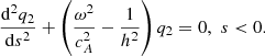
5.3. Case III
More generally, for non-degenerate cases the cut-off frequencies Ω1 and Ω2 are different from 0. Here we consider an example of a non-degenerate case with both A and cA/A being variable, as shown in Fig. 2. In the lower atmosphere the Alfvén speed increases and the field lines expand with a scale height of h/2. The second Klein–Gordon equation is reduced to
 (38)
(38)
By introducing the new variables
 (39)
(39)
we transform Eq. (38) into a second-order ordinary differential equation with constant coefficients:
 (40)
(40)
Equation (40) has solutions of the form 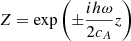 . The general solution of the original Eq. (38) is given by
![Mathematical equation: $$ \begin{aligned} q_2=\sqrt{\frac{4\pi c_{A}}{h }}\left[a\exp {\left(\frac{ih\omega }{2c_{A}} \right)}+b\exp {\left(-\frac{ih\omega }{2c_{A}} \right)} \right]. \end{aligned} $$](/articles/aa/full_html/2024/11/aa51507-24/aa51507-24-eq64.gif) (41)
(41)
The wave energy flux corresponding to the above solution (41) remains finite for all real frequencies. The constants outside the brackets in Eq. (41) ensure that the same amount of upgoing energy flux from the photosphere is produced in all three cases (see Sect. 7).
The magnetic field perturbation in the lower atmosphere, bφ, is determined from Eq. (21):
![Mathematical equation: $$ \begin{aligned} b_\varphi = \frac{\sqrt{B_s}}{c_{A}}\sqrt{\frac{4\pi c_{A}}{h }}\left[a\exp {\left(\frac{ih\omega }{2c_{A}} \right)}+b\exp {\left(-\frac{ih\omega }{2c_{A}} \right)} \right]. \end{aligned} $$](/articles/aa/full_html/2024/11/aa51507-24/aa51507-24-eq65.gif) (42)
(42)
The velocity perturbation, vφ, is determined from the equation of motion (11):
 (43)
(43)
Using the obtained expression (41) for q2, we find the velocity perturbation in the region s < 0:
![Mathematical equation: $$ \begin{aligned} v_\varphi =-\frac{1}{\sqrt{B_s}}\sqrt{\frac{4\pi c_{A}}{h}}\left[a\exp {\left(\frac{ih\omega }{2c_{A}} \right)}-b\exp {\left(-\frac{ih\omega }{2c_{A}} \right)} \right]. \end{aligned} $$](/articles/aa/full_html/2024/11/aa51507-24/aa51507-24-eq67.gif) (44)
(44)
The solutions in the upper atmosphere, s > 0, are again required to represent an outgoing wave. They are determined by the expressions (35) and (36) with a different constant coefficient  . Using the continuity conditions for bφ and vφ at the interface s = 0, we have
![Mathematical equation: $$ \begin{aligned} \sqrt{\frac{4\pi c_{A0}}{h }}\left[a\exp {\left(\frac{ih\omega }{2c_{A0}} \right)}+b\exp {\left(-\frac{ih\omega }{2c_{A0}} \right)} \right] = \tilde{c}, \nonumber \\ -\sqrt{\frac{4\pi c_{A0}}{h }}\left[a\exp {\left(\frac{ih\omega }{2c_{A0}} \right)}-b\exp {\left(-\frac{ih\omega }{2c_{A0}} \right)} \right] = - \tilde{c}. \end{aligned} $$](/articles/aa/full_html/2024/11/aa51507-24/aa51507-24-eq69.gif) (45)
(45)
From the set of equations (45) we have b = 0. We show in Sect. 7 that the obtained result indicates an absence of any downgoing wave energy flux for case III.
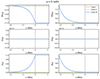 |
Fig. 4. Comparison of the velocity, vϕ, and magnetic field, bϕ, perturbations for a zero frequency wave corresponding to vortex motion. Both the real and imaginary components, as well as the amplitudes are shown. The dotted vertical line indicates the interface between the lower and the upper regions. |
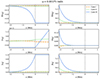 |
Fig. 5. Comparison of the velocity, vϕ, and magnetic field, bϕ, parameters for a low-frequency wave at ω = 0.00175 rad s−1 corresponding to a period of 1 hour. Both the real and imaginary components, as well as the amplitudes are shown. |
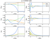 |
Fig. 6. Comparison of the velocity, vϕ, and magnetic field, bϕ, parameters for a high-frequency wave at ω = 0.209 rad s−1 corresponding to a period of 30 s. The real and imaginary components of the perturbations, as well as their amplitudes are shown. |
6. Comparison of the perturbations
Based on the obtained solutions in the previous section, we compare the velocity and magnetic field perturbations for the three cases. The SciPySpecial package is used to calculate the Hankel functions. The spatial profiles of the solutions are plotted between the photosphere at s = −2 Mm and the corona at s = 1 Mm. The coronal base lies at s = 0 Mm and is indicated with a dotted vertical line.
A scale height of h = 869.5 km is used for the plots. This is to allow the equilibrium parameters between the photosphere at s = −2 Mm and the coronal base at s = 0 Mm to be consistent with those shown in Fig. 2: a density and magnetic field decrease by 8 and 2 orders of magnitude, respectively, and a corresponding Alfvén speed increase by two orders of magnitude, from 10 to 1000 km s−1. The field lines expand by a factor of 10 for case I, a factor of 1000 for case II, and a factor of 100 for case III. It should be noted that the present model is restricted to a constant scale height. However, the actual scale height in the solar atmosphere is expected to vary with temperature.
In order to correctly compare the spatial behaviour of the Alfvén waves and their amplitudes, we have assumed that the amount of upward wave energy flux from the photosphere does not depend on the field line geometry in the atmosphere above. We show in the next section that |a|2 is a measure of the upward energy flux in the lower region. Therefore, the solutions of the linearised equations are normalised with respect to the constant a and are displayed in arbitrary units.
A torsional Alfvén wave with zero frequency does not propagate and instead forms a twisted steady-state configuration of the magnetic field, which can resemble a vortex in the plasma. The twist in the magnetic field induces a rotational motion of the plasma around the vertical symmetry axis, similar to a vortex in traditional fluid dynamics. While a vortex in fluid dynamics typically refers to the swirling motion of fluid around a central core, a zero-frequency torsional Alfvén wave can produce a similar swirling motion in a magnetised plasma, where the magnetic field lines themselves are twisted.
Figure 4 displays the behaviour of the perturbations with zero frequency representing a vortex. No vortical motions are observed for cases I and II. However, case III displays a vortical motion that reaches the corona. For cases I and II the upgoing energy flux is balanced by the downgoing flux, whereas case III exhibits no downgoing energy flux due to the particular magnetic field geometry (see Sect. 7). Vortical motions have been detected at different atmospheric heights in numerical simulations and in solar observations (Bonet et al. 2008; Battaglia et al. 2021; Silva et al. 2024). Only the real parts of the perturbations are present. There is an increase in the velocity perturbation and a decrease in the magnetic field perturbation from the photosphere to the corona.
The imaginary parts of the perturbations appear as the frequency begins to increase. Figure 5 shows the real and imaginary parts of vϕ and bϕ for the three cases in a low-frequency oscillation regime, ω = 0.00175 rad s−1. The upper panels show the real parts of vϕ and bϕ, the middle panels show their imaginary parts, and the lower panels display the corresponding amplitudes.
The plots show no oscillations in vϕ or bϕ. Instead, their spatial profiles are characterised by a continuous increase or a decrease between the photosphere and the coronal base.
The amplitudes in vϕ increase with distance s, whereas bϕ decreases in magnitude. Case III possesses the largest increase in vϕ, especially in the real part. The corresponding magnetic field in the lower atmosphere is comparatively high among the three cases. We show in the next section that this distinctive behaviour for case III is consistent with the wave energy flux having no downgoing component. Cases I and II both end up at the same low values at the coronal base at s = 0 Mm. In the lower region, s < 0 Mm, their values vary; the magnetic field for case II is higher.
Figure 6 displays the spatial profiles for vϕ and bϕ for a higher frequency oscillation of 0.209 rad s−1 corresponding to a period of 30 s. The three cases still display an increase in |vφ| and a decrease in |bφ| with distance s, with case III showing the largest increase. The imaginary parts of the perturbations increase with increasing frequency. In contrast to Figs. 4 and 5 for the low-frequency cases, the spatial profiles in Fig. 6 are more similar with moderate variations from the photosphere to the corona. This trend can be explained by the gradual decrease in the downgoing flux with increasing frequency for cases I and II (see Sect. 7). Another feature of Fig. 6 corresponding to a higher frequency is the oscillatory nature of the curves. Case III does not show oscillations in the magnitude plots as the real and imaginary components are out of phase.
Figures 4–6 demonstrate that the oscillatory nature of the perturbations becomes more prominent with increasing frequency. This behaviour is consistent with the predictions of the WKB theory. In the WKB approximation, the solutions of Eq. (23) can be expressed in the following form:
 (46)
(46)
Here Ωi represent the corresponding cut-off frequencies. At high frequencies, the difference Ωi2 − ω2 is negative and the solutions become oscillatory, which is consistent with the profiles of the curves in Figs. 4–6. At low frequencies the difference Ωi2 − ω2 is positive, and leads to non-oscillatory solutions.
In certain physical contexts, non-oscillatory solutions represent evanescent waves, which decay exponentially with distance from a localised source. In the present context, the non-oscillatory solutions contain both exponentially growing and decaying terms corresponding to the plus and minus signs in Eq. (46). These solutions contrast with the more familiar oscillatory wave solutions, which describe propagating waves.
7. The wave energy flux
In the previous section we explored the spatial profiles of the velocity and the magnetic field perturbations as well as the amplitudes in the solar atmosphere for three different cases. To further understand how the wave amplitudes in the corona are affected by the field line geometry, we derive expressions for the wave energy flux and establish relationships between the flux and the amplitude for each case.
Equations (11) can be combined to derive an equation of wave energy (Taroyan & Williams 2016; Taroyan et al. 2021).
 (47)
(47)
where
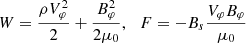 (48)
(48)
are the wave energy density and the wave energy flux, respectively.
A similar equation of energy can be derived for the real parts of the perturbations using the real parts of equations (11). The result is
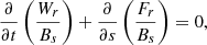 (49)
(49)
where
 (50)
(50)
By taking a time average over a single wave period we have
 (51)
(51)
For the left-hand side we have
 (52)
(52)
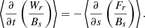
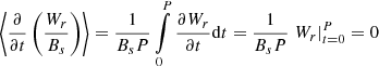
because the variable Wr is sinusoidal in time. Therefore, for the time-averaged energy flux on the right-hand side of Eq. (51) we have
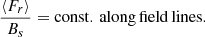 (53)
(53)
In practice, it is more convenient to deal with the complex variables rather than their real parts. We therefore express the flux, Fr, through the complex perturbations, vφ and bφ:
![Mathematical equation: $$ \begin{aligned} \frac{\langle F_r \rangle }{B_s}&= -\frac{1}{\mu _0 P}\int \limits _0^P \mathfrak{R} {(V_\varphi )} \mathfrak{R} {(B_\varphi )} \mathrm{d}t \nonumber \\&= -\frac{1}{4\mu _0 P}\int \limits _0^P \left[ v_\varphi \exp \left( i\omega t \right) + v_\varphi ^* \exp \left( - i\omega t \right)\right] \nonumber \\&\times \left[ b_\varphi \exp \left( i\omega t \right) + b_\varphi ^* \exp \left( - i\omega t \right)\right] \mathrm{d}t = -\frac{1}{2\mu _0 }\mathfrak{R} {\left(v_\varphi ^* b_\varphi \right)}. \end{aligned} $$](/articles/aa/full_html/2024/11/aa51507-24/aa51507-24-eq78.gif) (54)
(54)
Here the asterisk (*) denotes complex conjugation, and the integral is evaluated using the relationship between period and frequency, P = 2π/ω. Combining Eqs. (53) and (54) we obtain
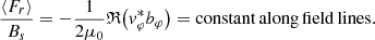 (55)
(55)
The obtained relationship (55) is valid for all s and can be used to derive expressions for the energy flux in each of the three cases shown in Table 1. This derivation also verifies that the ratio of the energy flux to the magnetic field strength, Bs, is conserved along the field lines.
Previous applications of the conservation law (55) mainly focused on models with a uniform magnetic field (Hollweg et al. 1982; Tsap & Kopylova 2021). Equation (55) can be used to explore the relationships between the cut-off frequencies, the wave energy flux, and the corresponding amplitudes in general magnetic field geometries.
7.1. Case I
The expressions (25) and (27) for the velocity and magnetic field perturbations, vφ and bφ, in the region s < 0 can be substituted in the formula (55) for the energy flux to obtain
![Mathematical equation: $$ \begin{aligned} \frac{\langle F_r \rangle }{B_s}&= -\frac{\omega }{2\mu _0}\mathfrak{R} {\left(v_\varphi ^* b_\varphi \right)} \nonumber \\&=\frac{\omega }{2\mu _0 c_{A}}\mathfrak{R} {\left[i(a^* H_0^{(1)*}+b^* H_0^{(2)*})(a H_1^{(1)}+b H_1^{(2)})\right]} = \frac{\omega }{2\mu _0 c_{A}}\nonumber \\&\times \mathfrak{R} {\left[i(a^* J_0 - ia^* Y_0 +b^* J_0 +i b^* Y_0)(a J_1+iaY_1 + b J_1 -ibY_1)\right]}\nonumber \\ &=\frac{\omega }{2\mu _0 c_{A}}\mathfrak{R} {\left[i|a|^2\left(J_0 J_1+iJ_0Y_1-iY_0J_1+Y_0Y_1\right)\right]} \nonumber \\&+\frac{\omega }{2\mu _0 c_{A}}\mathfrak{R} {\left[i|b|^2\left(J_0 J_1-iJ_0Y_1+iY_0J_1 + Y_0Y_1\right)\right]}\nonumber \\&+\frac{\omega }{2\mu _0 c_{A}}\mathfrak{R} {\left[ia^*b\left(J_0 J_1-iJ_0Y_1-iY_0J_1 - Y_0Y_1\right)\right]} \nonumber \\&+\frac{\omega }{2\mu _0 c_{A}}\mathfrak{R} {\left[iab^*\left(J_0 J_1 + iJ_0Y_1+iY_0J_1 - Y_0Y_1\right)\right]}, \end{aligned} $$](/articles/aa/full_html/2024/11/aa51507-24/aa51507-24-eq80.gif) (56)
(56)
where the arguments of the functions,  , are omitted for brevity. The sum of the last two terms in (56) is 0 because ℜ(iz) + ℜ(iz * ) = 0. Therefore,
 (57)
(57)
Using the well-known property of the Wronskian for the Bessel functions, W(J0, Y0) = J1Y0 − J0Y1 = 2π/z, where z represents the argument, we obtain
 (58)
(58)
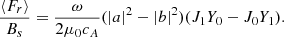
A similar expression was presented by Hollweg (1978), and it demonstrates that the ratio of the time-averaged energy flux to the field strength, ⟨Fr⟩/Bs, is conserved along the magnetic field lines. The formula can be interpreted as the difference between the upward and downward fluxes. In the present paper the net flux vanishes when upward and downward fluxes balance each other.
On the other hand, for the upper atmosphere, s > 0, we have the expressions (29). The ratio of the flux to the background magnetic field can therefore be expressed in an alternative format:
 (59)
(59)
Therefore, the net wave energy flux can be expressed either as the difference between the upward and downward fluxes in the lower atmosphere (58) or as an upward flux in the upper atmosphere (59). The latter expression establishes a direct link between the energy flux and the amplitudes in the corona.
7.2. Case II
The expressions (33) and (34) for the magnetic field and velocity perturbations, bφ and vφ, in the region s < 0 can be substituted in the formula for the energy flux to obtain
![Mathematical equation: $$ \begin{aligned} \frac{\langle F_r \rangle }{B_s}&= -\frac{1}{2\mu _0}\mathfrak{R} {\left(v_\varphi ^* b_\varphi \right)} \nonumber \\&=-\frac{\omega }{2\mu _0 c_{A}}\mathfrak{R} {\left[i(a^* H_1^{(1)*}+b^* H_1^{(2)*})(a H_0^{(1)}+b H_0^{(2)})\right]} = -\frac{\omega }{2\mu _0 c_{A}}\nonumber \\&\times \mathfrak{R} {\left[i(a^* J_1 - ia^* Y_1 +b^* J_1 +i b^* Y_1)(a J_0+iaY_0 + b J_0 -ibY_0)\right]}\nonumber \\ &=-\frac{\omega }{2\mu _0 c_{A}}\mathfrak{R} {\left[i|a|^2\left(J_0 J_1+iJ_1Y_0-iY_1J_0+Y_1Y_0\right)\right]} \nonumber \\&+\frac{\omega }{2\mu _0 c_{A}}\mathfrak{R} {\left[i|b|^2\left(J_0 J_1-iJ_1Y_0+iY_1J_0 + Y_0Y_1\right)\right]}\nonumber \\&+\frac{\omega }{2\mu _0 c_{A}}\mathfrak{R} {\left[ia^*b\left(J_0 J_1-iJ_1Y_0-iY_1J_0 - Y_0Y_1\right)\right]} \nonumber \\&+\frac{\omega }{2\mu _0 c_{A}}\mathfrak{R} {\left[iab^*\left(J_0 J_1 + iJ_1Y_0+iY_1J_0 - Y_0Y_1\right)\right]}, \end{aligned} $$](/articles/aa/full_html/2024/11/aa51507-24/aa51507-24-eq85.gif) (60)
(60)
where the arguments of the functions,  , are once again omitted for brevity. As in the previous case, the sum of the last two terms in (60) is 0 because ℜ(iz) + ℜ(iz * ) = 0. Combining this with the expression for the Wronskian, W(J0, Y0) = J1Y0 − J0Y1 = 2π/z, where z represents the argument, we obtain the same expression (58) derived for the previous case. It confirms that the ratio of the time-averaged energy flux to the field strength is conserved along the magnetic field lines, in agreement with (55).
A procedure similar to the one for case I can be carried out to establish expression (59) for case II. Therefore, expressions (58) and (59) are applicable to both degenerate cases I and II.
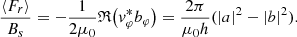
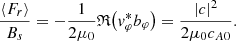
7.3. Case III
The magnetic field and velocity perturbations, bφ and vφ, in the lower atmosphere, s < 0, are given by the expressions (42) and (44). In Sect. 5, we establish that the coefficient b = 0 when the perturbation in the upper atmosphere is outgoing. Therefore, the following expression is obtained for the energy flux:
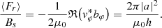 (61)
(61)
The above formula indicates that for the field line expansion representative of case III there is only an upward flux of energy. Using the solutions in the region s > 0 the same energy flux can be expressed in the form (59) with a different constant  .
.
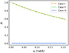 |
Fig. 7. Ratio of the downgoing to upgoing energy fluxes as a function of frequency. The overlaying curves indicate that the ratio, R, is identical for cases I and II. |
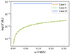 |
Fig. 8. Comparison of the time-averaged flux (⟨Fr⟩/Bs,) for the three cases over a range of frequencies up to a frequency of 0.209 rad s−1 representing a period of 30 s. |
7.4. Comparison of fluxes
The three principles set out in Sect. 5 allow us to construct physically acceptable solutions and to compare the wave amplitudes and the corresponding energy fluxes for the three different cases. Hollweg (1978) introduced the ratio of the downgoing energy flux to the upgoing energy flux,  . Previous theoretical studies suggested that vortices and low-frequency waves are strongly suppressed in the atmosphere (Hollweg 1978; Leer et al. 1982; Tsap & Kopylova 2021).
Figure 7 demonstrates the change in the flux ratio, R, with frequency, ω. It gradually decreases with increasing frequency as the proportion of downgoing flux decreases, and the waves transfer more energy into the upper atmosphere. Cases I and II are identical, as they are both given by Eq. (30).
On the other hand, for case III R = 0, indicating no downward flux, in agreement with the coefficient b being 0 from Equation (45). The energy flux enters the corona unhindered. This behaviour is consistent across the entire frequency spectrum.
The ratio of the time-averaged energy flux to the background field (55) is plotted in Fig. 8. The three cases are shown on log scales for various frequencies up to a frequency of 0.2 rad s−1 or a corresponding period of 30 s. Most notably, it can be seen for case III that the flux is significantly higher than the fluxes for cases I and II, especially at low frequencies. Cases I and II have the same fluxes, which is in agreement with the ratio R being the same. Both vanish in the limit of ω = 0, whereas the flux for case III does not change with frequency and remains consistently high. The fluxes for the three cases merge when the frequency increases because the proportion of the downgoing flux becomes small.
8. Summary and conclusions
The role of Alfvén waves in heating solar or stellar atmospheres and in wind acceleration remains one of the most important questions in solar and stellar physics. Conclusions based on theoretical models suggest that low-frequency Alfvén waves, which are the least susceptible to damping (Zaqarashvili et al. 2013), are unable to transport sufficient amounts of energy to the upper atmosphere of the Sun: a strong downward flux of wave energy is developed due to strong spatial gradients.
These views have been challenged by recent observations, which indicate the important role of these waves in the dynamics and energetics of the upper atmosphere (De Pontieu et al. 2014). Additionally, both observations and simulations indicate that vortices and swirling motions can lead to efficient transport of energy with subsequent heating (Bonet et al. 2008; Wedemeyer-Böhm et al. 2012; Breu et al. 2023). Revised models are required to reassess established views on wave behaviour and to reconcile observations and simulations with theory.
In the present paper we addressed the role of the magnetic field line geometry. It was shown that the propagation of Alfvén waves in arbitrary magnetic field geometries is governed by the Klein–Gordon equations for the magnetic field and velocity perturbations. The obtained results demonstrate that the energy flux reaching the corona and the corresponding perturbation amplitudes strongly depend on the magnetic field line expansion rate in the lower atmosphere. The flux is suppressed when for a given expansion rate either of the governing Klein–Gordon equations becomes degenerate and the corresponding cut-off frequency vanishes. A strong downward flux is developed that balances the upgoing flux (i.e. the ratio of the downgoing to upgoing fluxes, R = 1). This may explain why low-frequency Alfvén waves and vortices do not transport sufficient energy to heat the atmosphere in commonly adopted models. Examples include models based on a uniform magnetic field, a thin flux tube, or a radially expanding field. As a counterexample, a model is constructed where none of the cut-off frequencies vanish, and the Klein–Gordon equations remain non-degenerate, and lead to large perturbation amplitudes.
The energy flux is proportional to the perturbation amplitudes. Expressions for the time-averaged flux are derived and compared for three different cases. These cases have different expansion rates for the background magnetic field in the lower atmosphere. For cases I and II the flux has both downgoing and upgoing components, whereas the intermediate case III only has an upward component.
The amplitudes and the associated energy flux are strongly suppressed when the cut-off frequencies are zero. The cut-off frequencies mark the transition from higher frequency propagating waves to lower frequency growing and decaying waves. A vanishing cut-off frequency implies that even at low frequencies the solutions to the corresponding Klein–Gordon equations have an oscillatory behaviour. These propagating waves are reflected off the interface between the lower and the upper layers. A strong downward flux associated with the reflected counterpart balances the upward flux. Therefore, the amplitudes of the vortices and low-frequency waves become suppressed, in agreement with Figs. 4 and 5. Reflection is less efficient at higher frequencies (Fig. 7), and, therefore, the wave amplitudes and the energy flux reaching the corona increase with increasing frequency for cases I and II (see Figs. 6 and 8).
The intermediate case III demonstrates that non-zero cut-off frequencies in the Klein–Gordon equations are associated with large perturbation amplitudes and an energy flux that is significantly higher compared to the degenerate cases. The perturbations do not propagate and there is no reflection at the interface. The solutions have growing and decaying spatial profiles. The magnetic field perturbation decreases with distance, whereas the velocity perturbation increases as the energy flux should be conserved.
An increase in the velocity perturbations with increasing height (Fig. 4) is consistent with the presence of swirls and torsional motions in simulations and observations of the solar atmosphere (De Pontieu et al. 2014; Battaglia et al. 2021; Silva et al. 2024). When the frequency of the perturbations increases they become more oscillatory. The net energy flux remains high across the entire frequency spectrum as there is no downgoing component.
When Alfvénic motions are confined to a symmetry axis, they are usually seen to be highly reflective. This conclusion is also valid for models with a uniform magnetic field. The counterexample presented in this study shows the important role of the magnetic field line geometry. The energy flux reaching the corona can be consistently high across the entire frequency spectrum.
We focused on a particular field line geometry with different expansion rates in the lower atmosphere and exponential spatial profiles corresponding to a constant scale height. We need to ask the question of how sensitive the obtained results are to the background atmosphere. Future studies should look at wave propagation in an atmosphere with a more complex magnetic field line geometry. The preceding discussion is based on the general properties of the Klein–Gordon equations. We could therefore argue that the link between the cut-off frequencies and the energy flux carried by the Alfvén waves should hold both in simple and in more complex structures. There should be efficient transfer of energy (even if not 100%) as long as the cut-off frequencies do not vanish and there is no degeneracy in the corresponding Klein–Gordon equations.
The present study is restricted to the linear regime. An important question is how non-linearity can affect the transfer of energy flux and the reflectivity of the Alfvén waves. As the wave amplitude grows, Alfvén waves can become distorted, leading to steepening and the formation of shock-like structures. Non-linear interactions can also lead to the coupling of Alfvén waves with other wave modes, such as fast and slow magnetoacoustic waves, which can alter the reflectivity (Hollweg et al. 1982; Matsumoto & Shibata 2010). These coupled modes may have different reflectivity characteristics than pure Alfvén waves.
The transition from linear to non-linear behaviour is expected to lead to a more complex interaction with the solar atmosphere, where more energy is dissipated or converted into other forms. Both long- and short-period waves can experience non-linear effects, but short-period waves are more likely to steepen and dissipate. Detailed studies in the non-linear regime with different field line geometries would be required for more accurate conclusions.
Acknowledgments
T. Borradaile would like to thank the STFC for their financial support (ST/S505225/1).
References
- Alfvén, H. 1942, Nature, 150, 405 [Google Scholar]
- Alielden, K., & Taroyan, Y. 2022, ApJ, 935, 66 [NASA ADS] [CrossRef] [Google Scholar]
- An, C. H., Musielak, Z. E., Moore, R. L., & Suess, S. T. 1989, ApJ, 345, 597 [NASA ADS] [CrossRef] [Google Scholar]
- Aschwanden, M. J. 2019, New Millennium Solar Physics (New York: Springer), 458 [Google Scholar]
- Battaglia, A. F., Canivete Cuissa, J. R., Calvo, F., Bossart, A. A., & Steiner, O. 2021, A&A, 649, A121 [NASA ADS] [CrossRef] [EDP Sciences] [Google Scholar]
- Bonet, J. A., Márquez, I., Sánchez Almeida, J., Cabello, I., & Domingo, V. 2008, ApJ, 687, L131 [Google Scholar]
- Breu, C., Peter, H., Cameron, R., & Solanki, S. K. 2023, A&A, 675, A94 [NASA ADS] [CrossRef] [EDP Sciences] [Google Scholar]
- Cally, P. S. 2012, Sol. Phys., 280, 33 [NASA ADS] [CrossRef] [Google Scholar]
- De Pontieu, B., Rouppe van der Voort, L., McIntosh, S. W., et al. 2014, Science, 346, 1255732 [Google Scholar]
- Ferraro, C. A., & Plumpton, C. 1958, ApJ, 127, 459 [Google Scholar]
- Ferraro, V. C. A. 1954, ApJ, 119, 393 [NASA ADS] [CrossRef] [Google Scholar]
- Gary, G. A. 2001, Sol. Phys., 203, 71 [Google Scholar]
- Hollweg, J. V. 1978, Sol. Phys., 56, 305 [Google Scholar]
- Hollweg, J. V. 1984, ApJ, 277, 392 [Google Scholar]
- Hollweg, J. V., Jackson, S., & Galloway, D. 1982, Sol. Phys., 75, 35 [NASA ADS] [CrossRef] [Google Scholar]
- Jess, D. B., Mathioudakis, M., Erdélyi, R., et al. 2009, Science, 323, 1582 [Google Scholar]
- Leer, E., Holzer, T. E., & Fla, T. 1982, Space Sci. Rev., 33, 161 [Google Scholar]
- Liu, J., Nelson, C. J., Snow, B., Wang, Y., & Erdélyi, R. 2019, Nat. Commun., 10, 3504 [Google Scholar]
- Matsumoto, T., & Shibata, K. 2010, ApJ, 710, 1857 [NASA ADS] [CrossRef] [Google Scholar]
- McIntosh, S. W., de Pontieu, B., Carlsson, M., et al. 2011, Nature, 475, 477 [Google Scholar]
- Morgan, H., & Korsós, M. B. 2022, Sol. Phys., 297, 102 [NASA ADS] [CrossRef] [Google Scholar]
- Murawski, K., & Musielak, Z. E. 2010, A&A, 518, A37 [NASA ADS] [CrossRef] [EDP Sciences] [Google Scholar]
- Noble, M. W., Musielak, Z. E., & Ulmschneider, P. 2003, A&A, 409, 1085 [NASA ADS] [CrossRef] [EDP Sciences] [Google Scholar]
- Parker, E. N. 1991, ApJ, 372, 719 [NASA ADS] [CrossRef] [Google Scholar]
- Roberts, B. 2004, ESA Special Publ., 547, 1 [NASA ADS] [Google Scholar]
- Routh, S., Musielak, Z. E., Sundar, M. N., Joshi, S. S., & Charan, S. 2020, Ap&SS, 365, 139 [NASA ADS] [CrossRef] [Google Scholar]
- Ruderman, M. S., Verth, G., & Erdélyi, R. 2008, ApJ, 686, 694 [Google Scholar]
- Silva, S. S. A., Verth, G., Rempel, E. L., et al. 2024, ApJ, 963, 10 [NASA ADS] [CrossRef] [Google Scholar]
- Solanki, S. K., Inhester, B., & Schüssler, M. 2006, Rep. Progr. Phys., 69, 563 [CrossRef] [Google Scholar]
- Soler, R., Terradas, J., Oliver, R., & Ballester, J. L. 2017, ApJ, 840, 20 [Google Scholar]
- Soler, R., Terradas, J., Oliver, R., & Ballester, J. L. 2019, ApJ, 871, 3 [Google Scholar]
- Taroyan, Y., & Erdélyi, R. 2008, Sol. Phys., 251, 523 [CrossRef] [Google Scholar]
- Taroyan, Y., Hovhannisyan, G., & Sumner, C. 2021, MNRAS, 506, L64 [NASA ADS] [CrossRef] [Google Scholar]
- Taroyan, Y., & Williams, T. 2016, ApJ, 829, 107 [NASA ADS] [CrossRef] [Google Scholar]
- Tsap, Y., & Kopylova, Y. 2021, Sol. Phys., 296, 5 [NASA ADS] [CrossRef] [Google Scholar]
- Vernazza, J. E., Avrett, E. H., & Loeser, R. 1981, ApJS, 45, 635 [Google Scholar]
- Verth, G., Erdélyi, R., & Goossens, M. 2010, ApJ, 714, 1637 [NASA ADS] [CrossRef] [Google Scholar]
- Wedemeyer-Böhm, S., Scullion, E., Steiner, O., et al. 2012, Nature, 486, 505 [Google Scholar]
- Zaqarashvili, T. V., Khodachenko, M. L., & Soler, R. 2013, A&A, 549, A113 [NASA ADS] [CrossRef] [EDP Sciences] [Google Scholar]
All Tables
All Figures
|
Fig. 1. Axisymmetric poloidal magnetic field described by cylindrical coordinates and local orthogonal curvilinear coordinates. The angle ϕ representing the angle of rotation around the vertical symmetry axis, z, is not shown. The figure shows distance, s, along a curved magnetic field; the angle, θ, between the poloidal field and the vertical axis; and incremental increases δs and δa, along and across the poloidal field, respectively. |
| In the text | |
|
Fig. 2. Equilibrium parameters in the atmosphere. The panels on the left display the variation of density, Alfvén speed and magnetic field. The panels on the right show the radial distance, r = r(s), and the corresponding parameters that determine the cut-off frequencies Ω1 and Ω2. Logarithmic scales are used. |
| In the text | |
|
Fig. 3. Geometry of the magnetic field in the r − z plane. The field lines exponentially expand in the lower atmosphere and are vertical in the uniform upper atmosphere. |
| In the text | |
|
Fig. 4. Comparison of the velocity, vϕ, and magnetic field, bϕ, perturbations for a zero frequency wave corresponding to vortex motion. Both the real and imaginary components, as well as the amplitudes are shown. The dotted vertical line indicates the interface between the lower and the upper regions. |
| In the text | |
|
Fig. 5. Comparison of the velocity, vϕ, and magnetic field, bϕ, parameters for a low-frequency wave at ω = 0.00175 rad s−1 corresponding to a period of 1 hour. Both the real and imaginary components, as well as the amplitudes are shown. |
| In the text | |
|
Fig. 6. Comparison of the velocity, vϕ, and magnetic field, bϕ, parameters for a high-frequency wave at ω = 0.209 rad s−1 corresponding to a period of 30 s. The real and imaginary components of the perturbations, as well as their amplitudes are shown. |
| In the text | |
|
Fig. 7. Ratio of the downgoing to upgoing energy fluxes as a function of frequency. The overlaying curves indicate that the ratio, R, is identical for cases I and II. |
| In the text | |
|
Fig. 8. Comparison of the time-averaged flux (⟨Fr⟩/Bs,) for the three cases over a range of frequencies up to a frequency of 0.209 rad s−1 representing a period of 30 s. |
| In the text | |
Current usage metrics show cumulative count of Article Views (full-text article views including HTML views, PDF and ePub downloads, according to the available data) and Abstracts Views on Vision4Press platform.
Data correspond to usage on the plateform after 2015. The current usage metrics is available 48-96 hours after online publication and is updated daily on week days.
Initial download of the metrics may take a while.